globalization report 2016 - bertelsmann stiftung · globalization report 2016 who benefits most...
TRANSCRIPT

Globalization Report 2016Who benefits most from globalization?


Globalization Report 2016Who benefits most from globalization?
Michael Böhmer, Claudia Funke, Andreas Sachs, Heidrun Weinelt und Johann Weiß

55
Content
Executive Summary 6
1 Introduction 7
2 Who benefits most from globalization? 8 2.1 Summary of methodology 8
2.2 Globalization index results 9
2.3 Results of regression analyses of the correlation between
globalization and economic growth 12
2.4 Effects of globalization on growth 14
3 International competitiveness and export performance 21 3.1 Export performance 21
3.2 Change in global market shares at sector level 25
3.3 Constant Market Share Analysis 30
4 Bibliography 34
5 Appendix 35 5.1 Methodology for determining the globalization champion 35
5.2 Additional tables 40
5.3 Additional Figures 48
Figures and Tables 52 Figures 52
Tables 53
Imprint 54
6
The globalization report appears regularly and sets an
authoritative standard for the comprehensive analysis
of current globalization issues and global economic
development. The 2016 globalization report comes in two
parts. Building on the previous report, the first part focuses
on the question of to what extent different countries have
benefited from globalization in the past and to which
degree this is possible in the future. The second part
analyses the export performance and the development of
the international competitiveness of 42 globally important
economies.
The first part of the investigation creates a globalization
index which takes into account the economic, political and
social aspects of globalization. Subsequently, the index data
are used, together with a regression analysis, to quantify and
compare the impacts on growth caused by globalization in
the various countries. Then the country is identified which
has achieved the most growth as a result of globalization.
The most important results of the first part can be
summarised thus:
• If we add together the absolute differences in per capita
gross domestic product (GDP) between the scenario
without advancing globalization and the historically
observed development between 1990 and 2014, we find
Japan, Switzerland, Finland and Denmark at the top
of the tree. Germany is ranked below them alongside
smaller European countries. Bringing up the rear in terms
of absolute globalization gains per inhabitant are the
large emerging countries.
• The emerging countries’ low positions in terms of
absolute globalization gains – especially China’s – are
inter alia due to their weak per capita economic output in
the baseline year. Analysis of the relative globalization
gains shows a different picture: the average income gain
from globalization per inhabitant compared to per capita
Executive Summary
GDP in 1990 is about 17 % for China as against 5 % for
Germany and only 1.5 % for the USA.
The associated analysis of export performance and
the development of the global market shares of the 42
economies in total included in this study primarily reveals
the following aspects:
• Between 1995 and 2014, the group of emerging countries
grew massively in importance relative to the group of
developed countries. In this respect, it is clear that the
emerging countries’ growth is due to a large extent to
China’s huge growth. We must also acknowledge that
some developed countries – in particular, Germany – held
up well despite the new competition from the emerging
economies.
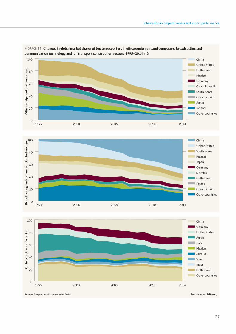
• There are also obvious differences at the sector level:
While in some sectors much more than half of globally
traded goods now come from emerging countries (such
as office equipment and computers or broadcasting
and communication technology), in other sectors the
established developed countries are still leading the way
(e.g. in the pharmaceutical industry and in aerospace
equipment construction).
• A constant market share analysis shows conclusively
that the rise of the emerging countries is primarily due
to their much improved competitiveness relative to the
average competitiveness of all economies.

7
The 2016 globalization report is divided into two parts. The
growth effect of globalization on a total of 42 economies
is analysed, based on the key question “Who benefits
most from globalization?” The aim of the investigation is
to establish for every highly developed economy and the
most important emerging countries to what extent they
were affected by increasing globalization between 1990 and
2014 and, where applicable, to what extent they benefited
from it. This approach reveals the big and small winners
of globalization and thus enables us to determine the
“globalization champion.”
Subsequently, we analyse the export performance of these
countries and the development of their global market
shares since 1995. In addition, a constant market share
analysis gives us information on the extent to which the
various economies’ competitiveness has developed relative
to the other countries examined. It reveals the factors on
the basis of which each global market share has developed.
1 Introduction

8
index is made up of sophisticated indicators illustrating
the economic, social and political aspects of globalization.2
A second phase brings the analysis of the causal relations
between globalization and economic development into
the foreground. The growth effect of globalization is also
quantified using regression analyses. This enables the effect
of individual influences on economic development to be
filtered out, while the effects of other drivers of economic
development are statistically estimated.
In the regressions, economic development is interpreted
as a variable in terms of the percentage growth of output
per inhabitant. The globalization index acted as the main
indicator. The regression results for this variable show how
strongly economic development is driven by globalization.
This knowledge of the sensitivity of economic growth per
inhabitant with regard to globalization is then used in
the next phase of the work in order to quantify individual
countries’ globalization-induced growth increases and on
this basis to determine the globalization champion.
Globalization-induced growth increases are quantified in
two sub-phases. Initially, a calculation is made for each
country of the growth rates which it would have had in the
event of a period of stagnation of globalization. Next, the
annual changes in the globalization index are multiplied by
the estimated globalization effect and subtracted from the
historical growth rate values.
Finally, based on the GDP at the start of the period in
question and applying the recently calculated growth
rates, a counterfactual growth trajectory is created for each
country to illustrate its economic development in the event
of a period of stagnation of globalization.
2 The selection of the indicators is in line with the KOF globalization index (see Dreher 2006).
In order to quantify the growth effects of globalization,
we have produced a globalization index and performed
an econometric study of the causal relations between
globalization and the economic development of the
economies included in this study.1 A synthesis of this
knowledge enables us to give rankings to the country-
specific changes in economic output due to globalization
and thus to select the globalization champion.
2.1 Summary of methodology
The detailed investigation of the causal relations between
globalization and economic development is the core of the
study. Our knowledge of these causal relations is used to
quantify the economic changes caused by globalization in
the ex post time period of 1990–2014. The section below
gives a brief overview of the approach. The appendix
to this study contains a detailed description of the
methodology.
In order to establish the globalization champion we used
the following steps:
1. Production of the globalization index
2. Investigating the causal relations between
globalization and economic development
3. Determining the globalization champion
In order to be able to quantify the economic influence of
globalization, this multi-layered process must be made
measurable. This is done in the first phase of the study
on the basis of a comprehensive globalization index. The
1 The economies investigated are the 42 countries in Prognos’ macroeconomic multi-country model, VIEW. This list of countries includes all the highly developed economies and large emerging countries which together make up over 90 % of global economic output.
2 Who benefits most from globalization?

9
Who benefits most from globalization?
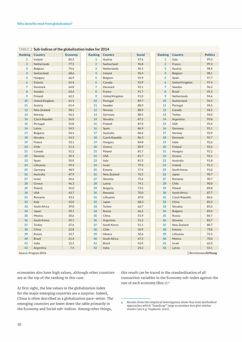
2.2 Globalization index results
The globalization index shows that with Ireland, the
Netherlands and Belgium at the top of the table, primarily
it is highly developed, well connected and mostly
smaller economies that display especially high levels of
globalization (Table 1).
Larger highly developed economies such as France, Spain,
Germany and Italy are in mid-table. Among this group,
the United Kingdom has the highest ranking. Bringing
up the rear in the globalization index are countries like
China, Brazil, Argentina and India – the major emerging
countries. These results are comparable to the results of
other globalization indices.3
The overall index is made up of the three Economy, Social
and Political sub-indices. A separate look at each sub-
index provides information on how the ranking is to be
assessed in the overall index (Table 2). By way of example,
the top positions held by Ireland, the Netherlands and
Belgium are due to their very high values in the Economy
and Social sub-indices. In the Political sub-index those
3 In the previous study “Globalization report 2014 – Who benefits most from globalization?” there is a detailed comparison of the globalization index with the New Globalization Index, the Ernst & Young, the Economic Intelligence Unit (EIU) and the KOF globalization indices.
By comparing historical values of GDP with the values
that arise from the counterfactual growth trajectory,
we can tabulate and compare the individual countries’
globalization-induced increases and decreases in growth.
The decisive factor in the final determination of the
globalization champion is which country was able to
achieve cumulatively over the whole period between 1990
and 2014 the largest gains in per capita GDP as a result of
globalization.
Table 1 Globalization index for 2014
Ranking Country Globalisation index Ranking Country Globalisation index
1 Ireland 88.87 22 Bulgaria 64.35
2 Netherlands 84.73 23 Greece 62.95
3 Belgium 83.57 24 Slovenia 62.10
4 Switzerland 79.41 25 Italy 61.38
5 Austria 76.07 26 Poland 61.27
6 Denmark 75.83 27 USA 61.25
7 Hungary 75.56 28 Chile 58.94
8 Sweden 75.05 29 Latvia 58.14
9 United Kingdom 74.59 30 Romania 58.04
10 Finland 73.15 31 Lithuania 57.93
11 Portugal 70.29 32 Israel 56.20
12 Norway 70.10 33 Japan 55.24
13 France 70.07 34 South Africa 50.92
14 Estonia 69.48 35 Turkey 48.73
15 Canada 68.37 36 South Korea 45.89
16 Czech Republic 68.19 37 Russia 43.79
17 Slovakia 67.00 38 Mexico 42.46
18 Spain 66.89 39 China 41.06
19 New Zealand 66.30 40 Brazil 40.34
20 Germany 65.66 41 Argentina 33.52
21 Australia 64.38 42 India 31.08
Source: Prognos 2016
10
Who benefits most from globalization?
this result can be traced to the standardisation of all
transaction variables in the Economy sub-index against the
size of each economy (Box 1).4
4 Results from the empirical investigation show that even methodical approaches which “handicap” large economies less give similar results (see e.g. Vujakovic 2010).
economies also have high values, although other countries
are at the top of the ranking in this case.
At first sight, the low values in the globalization index
for the major emerging countries are a surprise. Indeed,
China is often described as a globalization pace-setter. The
emerging countries are lower down the table primarily in
the Economy and Social sub-indices. Among other things,
Table 2 Sub-indices of the globalization index for 2014
Ranking Country Economy Ranking Country Social Ranking Country Politics
1 Ireland 85.5 1 Austria 97.6 1 Italy 99.3
2 Netherlands 77.5 2 Switzerland 96.8 2 France 99.3
3 Belgium 74.6 3 Netherlands 96.5 3 Austria 98.4
4 Switzerland 68.6 4 Ireland 96.4 4 Belgium 98.1
5 Hungary 66.9 5 Belgium 95.9 5 Spain 97.7
6 Estonia 65.4 6 Canada 93.9 6 United Kingdom 97.4
7 Denmark 64.8 7 Denmark 92.1 7 Sweden 96.2
8 Sweden 63.4 8 France 91.7 8 Brazil 95.5
9 Finland 62.2 9 United Kingdom 91.0 9 Netherlands 94.6
10 United Kingdom 61.5 10 Portugal 89.7 10 Switzerland 94.5
11 Austria 61.4 11 Sweden 88.9 11 Portugal 94.5
12 New Zealand 58.1 12 Norway 88.9 12 Canada 94.5
13 Norway 56.2 13 Germany 88.5 13 Turkey 94.0
14 Czech Republic 56.0 14 Slovakia 87.2 14 Argentina 93.8
15 Portugal 55.8 15 Finland 87.0 15 USA 93.4
16 Latvia 54.5 16 Spain 86.9 16 Germany 93.1
17 Bulgaria 54.4 17 Australia 86.6 17 Norway 92.9
18 Slovakia 54.3 18 Czech Republic 86.3 18 Denmark 92.7
19 France 53.1 19 Hungary 84.8 19 India 92.6
20 Chile 51.3 20 Greece 83.9 20 Finland 92.2
21 Canada 51.2 21 Poland 81.7 21 Hungary 92.2
22 Slovenia 50.4 22 USA 81.7 22 Greece 92.1
23 Spain 50.0 23 Italy 81.5 23 Australia 91.8
24 Lithuania 49.4 24 Israel 79.3 24 Ireland 91.3
25 Germany 48.9 25 Estonia 77.4 25 South Korea 91.0
26 Australia 47.9 26 New Zealand 76.5 26 Japan 90.7
27 Israel 46.6 27 Slovenia 75.6 27 Romania 90.7
28 Greece 46.3 28 Latvia 74.1 28 Chile 90.0
29 Poland 45.0 29 Bulgaria 73.5 29 Poland 89.8
30 USA 43.7 30 Romania 70.0 30 South Africa 87.7
31 Romania 43.2 31 Lithuania 69.0 31 Czech Republic 86.6
32 Italy 42.0 32 Japan 68.3 32 China 85.2
33 South Africa 39.8 33 Turkey 66.7 33 Slovakia 85.0
34 Japan 39.1 34 Russia 66.2 34 Bulgaria 85.0
35 Mexico 30.6 35 China 51.9 35 Russia 84.7
36 South Korea 29.1 36 Argentina 51.2 36 Slovenia 83.7
37 Turkey 27.6 37 South Korea 51.1 37 New Zealand 80.7
38 China 22.8 38 Chile 50.9 38 Estonia 73.8
39 Russia 22.7 39 Mexico 50.6 39 Lithuania 72.5
40 Brazil 21.4 40 South Africa 47.5 40 Mexico 70.0
41 India 12.5 41 Brazil 42.0 41 Israel 62.0
42 Argentina 7.5 42 India 25.2 42 Latvia 53.1
Source: Prognos 2016

11
Who benefits most from globalization?
Highly developed economies which are positioned in mid-
table in the overall index have the top rankings in the
Political sub-index. This is especially the case for Italy and
France. Spain and the United Kingdom are also near the top.
In the overall index and the sub-indices, Germany is only in
mid-table positions, even though the country has been the
unofficial “world champion exporter” for years.
In interpreting these results, we should note that high
or low values do not represent an assessment. They are
merely a measurement of the extent to which a country is
connected to the rest of the world (in each sub-area).
To classify the results of the globalization index or sub-
index it is helpful to give examples of some country-specific
differences for some of the indicators. This shows us that
Germany’s relatively low value in the globalization index is
at least partly due to economies of scale: Domestic markets
play a more important role for larger economies than for
smaller ones. Thus the value creation chains of companies
from smaller countries rely to a much greater extent on
international suppliers. In Germany, the total value of
exports and imports in 2014 was around 2.7 billion euros
– nine times as high as in the Czech Republic. In terms of
gross domestic product, the order is reversed: the Czech
Republic exported and imported goods amounting to 137 %
of its economic output. For Germany, this “openness” only
amounts to 69 %. Economies of scale also have clear effects
on other indicators.
Geographical features and the country-specific importance
of the financial sector also have an appreciable influence
on the rankings in the globalization index. In particular,
the Netherlands and Belgium have a very high degree of
openness due to the international importance of their
ports, Rotterdam and Antwerp. The importance of Ireland’s
capital, Dublin, as a financial centre means that the country
is in a top ranking position in terms of international capital
flows. In this context, the United Kingdom’s high value in
the Economy sub-index is a reflection of London’s strength
as a financial centre.
In general, a glance at the development of the globalization
index since 1990 indicates that the rankings have barely
changed in the last 24 years (Figure 1). Every economy
showed an upward movement in the 1990s. However, it
was similar for every country. Thus the leaders for the
entire period under observation have been Ireland, the
Netherlands and Belgium.
In the main, therefore, smaller, highly developed countries
are the most highly globalized countries in the world. Those
countries owe their high ranking partly to the high scores
their economic output gained for the economic indicators.
In contrast, the large European countries – with the
exception of the United Kingdom – occupy positions in mid-
table, which is mainly due to the average scores of their
economic indicators, enhanced by the high weighting of
the sub-index. The major emerging countries bring up the
rear in the globalization index but over time have shown an
above-average ability to catch up with the others.
box 1 China’s position in the globalization index
In the overall index, China is in 39th place. This result
is mainly due to China’s low score in the Economy sub-
index. This may be surprising, given China’s importance
to the global economy, but a glance at China’s scores for
the individual indicators gives an explanation. Firstly, we
must be clear that the Economy sub-index includes not
only transaction variables but also those indicators which
measure the limitations on transactions. Because of its
relatively restrictive trade policy for all four indicators,
China occupies one of the lowest rankings in this sub-
index. This applies most obviously to the capital controls
indicator. With a score of 3.5 for this indicator, China is
in fifth from last position of all countries in the index. For
comparison’s sake: the globalization index leaders such
as Ireland and the Netherlands score between 8 and 9 for
this indicator.
Secondly, China does not score very highly compared to
other economies in the “transaction variable” indicators.
This is the case for portfolio investments (9.1 % of GDP
– 42nd place), foreign direct investments (18 % of GDP
– 42nd place) and trade in services (5 % of GDP – 41st
place). Even in commodity trading, China, with 38 % of
GDP, is “only” in 35th place of all the countries in the
index. One of the main reasons for this is that, for the
globalization index, the absolute transaction variables of
a country are adjusted to take into account its GDP. For
example, in absolute terms, China accounts for over 3.9
billion euros of commodity trading – six times Belgium’s
trade volume; this puts it in second place after the United
States.

12
Who benefits most from globalization?
increased its globalization index by 0.53 per year between
1990 and 2014, 0.16 % was added to its annual per capita
growth rate through its increasing connectedness with the
rest of the world. As a whole, the average growth in per
capita GDP over that period was 1.37 %. Thus globalization
played an important role in this growth.
The other estimated results of the baseline specification
also show the expected signs. Per capita GDP, birth rate
and the indicator for the most recent global economic crisis
negatively influenced the estimate and all these results
are statistically significant. The coefficient of –8.60 for the
influence of economic output means that an increase in GDP
per inhabitant of 1 % leads to a decrease in per capita growth
of 0.086 % two years later. The same applies to fertility. For
this variable, an increase of 1 % corresponds to a fall in per
capita growth of 0.09 %. The estimated coefficient of –3.63
for the crisis years 2008 and 2009 means that per capita
economic growth in this period was about 3.6 % lower than
in the other period under observation. The estimated value
of investments as a share of GDP (0.17) also falls into line
with expectations.
The reliability of the estimates is tested using various
alternative regression parameters. The first alternative is
one where the growth effect of globalization is estimated
separately for various groups of countries but in other
2.3 Results of regression analyses of the correlation between globalization and economic growth
The correlation between globalization and economic growth
is quantified using regression analyses. This enables the
effect of individual influences on economic development
to be filtered out, while the effects of other drivers of
economic development are statistically estimated.
The regression results of the baseline specification (Table
3) form the basis of the investigation. Alongside the
globalization index – its main explanatory variable – the
baseline includes per capita GDP, birth rate, investments
and a crisis indicator for 2008 and 2009.5
The results demonstrate that globalization has a very
positive influence on the growth of per capita GDP. The
estimated coefficient of 0.31 means that an increase in
the globalization index of one point on average leads to
an increase in the growth of per capita GDP of 0.31 %. For
Germany, for example, this means that, since the country
5 The selection of the variables for the baseline specification is largely based on the significance of the growth effects of these determinants as demonstrated in the results. An endogenous variable – investments – is also included.
FIGURE 1 Developments in the globalization index for selected countries for the period 1990–2014
Source: Prognos 2016
IrelandNetherlandsBelgium
United Kingd.FranceGermanyItalyUSAJapan
RussiaChina
Indien
0
20
40
60
80
100
201420102005200019951990

13
Who benefits most from globalization?
one of the estimates significantly differs from 0.31.7 Thus
it is clear that the alternative parameter with estimates of
the growth impact of globalization that are specific to the
groups of countries does not produce significant additional
results. Furthermore, the estimated coefficients of the
other explanatory variables scarcely differ from those of the
baseline.
Depending on the baseline and the parameter for the
sensitivities specific to the groups of countries, additional
regressions with various combinations of explanatory
variables are tested as further alternatives. The results of
these regressions solidify the finding that the estimated
growth influences of globalization and those of the other
explanatory variables can be regarded as robust and reliable
(Table 17 and Table 18 in the Appendix).
7 The smallest p-value for two-sample t-tests is 0.01 for the group of large economies with a high per capita GDP. The next smallest value is 0.05 for the group of small economies with a high GDP. Thus the null hypothesis that the estimated sensitivity of growth to globalization is a value of 0.31 can be rejected only for the group of large economies with a high per capita GDP with a significance level of under 5 %.
respects the same explanatory variables are used. To that
end the economies included in this study are divided
according to GDP per capita in 1990 and the size of the
economy in 1990 (measured as GDP) into four large groups
of countries as similar as possible in size (Table 21 in
Appendix 5.2).6
The results show that all four country groups demonstrate
the same per capita growth sensitivity to globalization
(Table 3, column 3). Compared to the baseline, small
economies with low per capita GDP (0.38) have a somewhat
higher growth sensitivity to globalization while all the other
groups of countries have a slightly lower sensitivity. The
differences between the estimates are too small to allow
for meaningful interpretations – the more so since only
6 The division was carried out as follows: Firstly, all the countries in the study were divided in two by median GDP per capita in 1990. This was 10 050 euros. Next, the groups of countries thus created were each divided into two sub-groups by median GDP in 1990. This figure was 250 billion euros for the group of countries with a high GDP per capita and 95 billion euros for the group of countries with a small GDP per capita.
Table 3 Regression results of the determinants of economic growth per inhabitant
Dependent variable: Growth of per capita GDP in percent IV method with FE IV method with FE and country groups
Globalisation overall 0.31***
(0.08)
Globalisation for
· large economies with high per capita income 0.24***
(0.03)
· small economies with high per capita income 0.19**
(0.06)
· large economies with low per capita income 0.23
(0.15)
· small economies with low per capita income 0.38***
(0.10)
Per capita GDP of period before last (logarithmized) –8.60*** –8.27***
(1.34) (1.41)
Birth rate (logarithmized) –9.03*** –9.40***
(1.86) (2.56)
Investments (as % of GDP) 0.17* 0.15*
(0.08) (0.08)
Crisis indicator 2008–2009 –3.63*** –3.60***
(0.40) (0.39)
Number of observations 966 966
R² (centered) 0.375 0.385
N.B.: The symbols *, ** and *** show the significance of the estimates for the 10%, 5% and 1% levels. The figures in brackets are the standard errors by country clusters. All regressions contain a constant. FE = country-specific fixed effects
Source: Prognos 2016

14
Who benefits most from globalization?
2.4.1 Globalization champion determined using per capita income gains
Looking at the absolute per capita income gains due to
increasing globalization, we see that Japan is in first place
(Table 4).9 Therefore, from this perspective, Japan is the
globalization champion, followed by Switzerland, Finland
and Denmark. Ireland, Austria, Greece and Sweden are
other small European countries occupying places in the
top ten on the list. However, Germany – a large economy
– has also shown large per capita income gains and can
therefore count itself as one of the (bigger) winners of the
globalization process.
Places 11 to 24 are occupied primarily by Central European
countries or national economies with a gross domestic
product per capita that is high in comparison with the rest
of the world. Slovenia also provides a Central and Eastern
European country among these countries. It is noteworthy
that residents of large industrial nations have not benefited
equally from increasing global interconnectedness.
Globalization gains per capita in the United States are less
than half as high as those for Germany. France, Canada and
Spain have also benefited less from globalization.
The lower mid-range of globalization winners consists
primarily of nations from Central and Eastern Europe.
Bringing up the rear in terms of absolute globalization
gains per inhabitant are the large emerging countries.
Thus, in spite of the importance to them of large internal
markets and strong economic output for global economic
development, these countries do not number among the
main beneficiaries of globalization in the sense of absolute
per capita income gains.
9 In classifying the results properly it is important to note that the above investigation allows for no analysis of income distribution within a country. The globalization-induced income gains demonstrated refer exclusively to the population as a whole.
The overall result of the regression analysis demonstrates
that globalization has a stable and very positive influence
on the growth of per capita GDP. The robustness of
the estimates, in particular, increases our faith in the
regression results. The estimated sensitivity of per capita
growth using the baseline of 0.31 % per point on the
globalization index also acts as the main interim result of
this section. Based on this sensitivity, the globalization
champion is determined in the next section.
2.4 Effects of globalization on growth
Based on the above results, we examine to what extent
the countries in question benefited from increasing
globalization from 1990 to 2014. This analysis is based
on a comparison of the historical development of GDP
against a counterfactual scenario in which we assume
that globalization remained stagnant at its 1990 level.
In other words: we assume in the comparison scenario
that the globalization index remained at its 1990 level for
each country for all of the years from 1990 to 2014.8 As
metrics for the globalization effects, we use the cumulative
differences in per capita GDP over the entire period in
question. In interpreting the results, we must distinguish
between economic growth and cumulative income gains
(Box 2).
The globalization champion is the country the inhabitants
of which have benefited the most from increasing
globalization, taking into account the cumulative effects.
In line with this focus on the individual’s economic
situation, we also use the absolute income gains and the
absolute income gains weighted according to purchasing
power as two alternative key indicators to determine the
globalization champion.
In order to differentiate the results in relation to the various
starting positions and the various sizes of the individual
economies, the globalization-induced per capita income
gains are shown in relation to the GDP in 1990, as well as
the aggregated income gains of the entire economy.
8 For the counterfactual scenario, the development of per capita GDP is calculated using the following formula:
Where gt stands for the historical growth rate of GDP in %, POPt for population in year t and GIt for the globalization index value in year t. Next, the GDP itself is produced through the multiplication of per capita GDP with the historical population figures.
!"#!!"!!
=!"#!""#!"!!""#
∗ 1+!! − 0,31 ∗ (!"! − !"!!!)
100
!
!!!""!

15
Who benefits most from globalization?
FIGURE 2 Schematic representation of the change in gross domestic product and globalization-induced income gains
Source: Prognos 2016
95
100
105
110
115
120
125
130
135
109876543210
Income gainStagnant globalizationActual development
Per
cap
ita
GD
P
Time
box 2 Interpretation of globalization-induced income gains as a key indicator in determining the globalization champion
The stagnant globalization assumed for the
counterfactual scenario implies lower economic growth
and, therefore, a less favourable growth trajectory.
The year-on-year difference between the per capita
GDP under this alternative scenario and what actually
happened is the absolute economic gain (Figure 2).
In order to measure the cumulative effects of
globalization, these gains for each country are added
together for the entire 1990–2014 period. In this study
the amount calculated in this way is also described as the
“cumulative income gain due to increasing globalization.”
This amount should not be confused with the amounts
used in the national accounts such as disposable income.
Furthermore, we must distinguish between income
gains and changed growth rates. Thus a one-off
increase in the GDP growth rate itself produces income
gains which accumulate over the remaining period
under investigation even when growth rates do not
otherwise change over that period. In contrast, a one-off
globalization-related income gain has no implications for
the growth rate in the following years.

16
Who benefits most from globalization?
Another important issue arises for countries with
the highest globalization index values: Belgium, the
Netherlands and Ireland are not top of the table in terms
of per capita globalization gains. The reason for this is
that these economies have a high degree of connectedness
with the rest of the world but were not very dynamic in
the period under investigation. This result shows clearly
the significance of constant efforts to open up an economy
to the rest of the world – even, or especially, for highly
globalized countries.
Looking at the change over time gives us additional
information on how the globalization-related per capita
income gains should be assessed (Figures 13 to 16 in the
Appendix). This shows that the largest growth gains
occurred in the period from the mid-1990s to the middle of
the first decade of the 21st century. Globalization champion
Japan and the other main globalization winners had already
increased their per capita GDP at the beginning of the
period under investigation as a result of globalization. Thus
Table 4 Absolute per capita income gains due to
increasing globalization 1990–2014
Ranking Country Average annual per capita income gain from 1990 in euros*
Cumulative per capita income gain from 1990 in euros*
1 Japan 1,470 35,300
2 Switzerland 1,360 32,700
3 Finland 1,340 32,100
4 Denmark 1,210 29,100
5 Ireland 1,130 27,100
6 Germany 1,130 27,000
7 Israel 1,040 24,900
8 Austria 880 21,100
9 Greece 880 21,100
10 Sweden 850 20,400
11 South Korea 830 19,800
12 Italy 780 18,800
13 Australia 770 18,400
14 Portugal 770 18,400
15 Slovenia 710 17,000
16 New Zealand 700 16,900
17 Netherlands 690 16,500
18 United Kingdom 680 16,200
19 France 650 15,600
20 Canada 650 15,500
21 Spain 530 12,700
22 Belgium 500 11,900
23 United States 490 11,700
24 Estonia 440 10,600
25 Hungary 400 9,600
26 Norway 340 8,100
27 Lithuania 310 7,500
28 Chile 310 7,400
29 Slovakia 300 7,300
30 Poland 270 6,400
31 Latvia 260 6,300
32 Czech Republic 260 6,300
33 Turkey 200 4,800
34 Romania 190 4,500
35 South Africa 180 4,200
36 Bulgaria 170 4,000
37 Argentina 130 3,100
38 Mexico 130 3,000
39 Brazil 120 2,900
40 Russia 120 2,800
41 China 70 1,700
42 India 20 400
* actual prices in 2000; rounded values
Source: Prognos 2016
box 3 Comparison of current results with results in the 2014 globalization report
The globalization index used here was initially created
in 2014 and the globalization champion was determined
on that basis. What changes can we see when comparing
current results with the results from 2014?
In terms of absolute per capita income gains due to
increasing globalization over the period in question
(Table 4) the same countries as before are in the top
positions. Ireland has joined Japan, Switzerland, Finland
and Denmark in the top five, which has pushed Germany
down to number 6. However, the order has changed.
Japan is now at the top of the table (3rd place in the 2014
globalization report), followed by Switzerland (5th),
Finland (1st), Denmark (2nd) and Ireland (9th). There are
also differences in the absolute income gains: Compared
to the previous survey, Japan and Switzerland have seen
a large increase in cumulative growth, while Denmark
and Austria have seen a reduction. What do these results
mean?
Two variables vital for the calculation of the globalization
gains have changed for all countries. Firstly, the estimated
coefficient of the regression calculation is now 0.31. In
the previous globalization report, this value was 0.35,
based on the data then available. Both cases demonstrate

17
Who benefits most from globalization?
it is clear how important the changes in the early years of
the period under observation are for the overall results of
this investigation (Box 4).
Alongside the absolute income gains, the additional
purchasing power that arises for each economy as a result
is also important. For this reason, we analyzed income
gains per capita that were weighted according to purchasing
power as an alternative way to determine the globalization
champion (Table 5). Under this approach, Finland is in
top position. Also Greece is near the top, in second place
(previously 9th). In contrast, from this perspective Japan
slips down to 16th place.
that globalization has a very positive influence on the
growth of per capita GDP, although in the current
estimate the influence is slightly less. The extension of the
period under observation by three years had the same
effect on all countries.
In contrast, the changes in the globalization index turned
out differently for various countries. For some countries
such as the USA, the index values have not changed
noticeably in the three years since the study of the
1990–2011 period; however, for other countries there
have been noticeable changes. Thus Japan’s index value
has clearly increased in the last two years. In contrast,
the globalization index for the United Kingdom has
worsened noticeably since 2011. In some countries,
the globalization index also changed noticeably in the
preceding periods compared to the previous study: for
China between 1990 and 2001 and for Austria from 2000
to 2011. Various factors are responsible for the changes
in the index values. The fall in the United Kingdom’s
globalization index is mainly due to the slow development
of foreign trade and tighter capital flow controls in the
more recent past. Japan has significantly increased
its foreign investments and its degree of openness. In
addition, in the case of Japan, for example, exchange rate
fluctuations also play an important role. The changes in
the index value in periods further back in time are mainly
due to revised data.
Table 5 Per capita income gains due to increasing
globalization 1990–2014, weighted for purchasing power
Ranking Country Average annual per capita income
gain in euros, adjusted*
Cumulative per capita income gain in euros,
adjusted*
1 Finland 1.460 35.000
2 Greece 1.410 33.800
3 Ireland 1.280 30.600
4 Germany 1.270 30.400
5 South Korea 1.250 30.000
6 Switzerland 1.240 29.800
7 Slovenia 1.240 29.700
8 Israel 1.230 29.500
9 Portugal 1.190 28.500
10 Denmark 1.170 28.000
11 New Zealand 1.120 26.800
12 Austria 1.060 25.500
13 Estonia 1.060 25.400
14 Hungary 1.040 25.000
15 Italy 1.040 25.000
16 Japan 1.030 24.600
17 Australia 930 22.400
18 Sweden 850 20.500
19 Netherlands 840 20.100
20 Lithuania 830 19.800
21 Spain 780 18.700
22 Canada 780 18.700
23 France 750 18.100
24 Czech Republic 710 17.100
25 United Kingdom 700 16.900
26 Bulgaria 650 15.600
27 Romania 650 15.500
28 Latvia 640 15.400
29 Poland 630 15.100
30 Slovakia 630 15.000
31 Belgium 600 14.500
32 Chile 580 14.000
33 United States 490 11.700
34 Russia 450 10.800
35 South Africa 450 10.700
36 Turkey 440 10.600
37 Norway 330 7.800
38 Brazil 290 7.000
39 China 220 5.300
40 Mexico 190 4.600
41 Argentina 150 3.700
42 India 80 2.000
* adjusted for purchasing power in relation to the United States; actual prices in 2000; rounded values
Source: Prognos 2016

18
Who benefits most from globalization?
2.4.2 Globalization-induced per capita income gains compared to the starting point
Analysis of the per capita income gains compared to the
starting point of per capita GDP produces a very different
ranking of countries (Table 6). Economies which in 1990
had a low to medium ranking in terms of per capita GDP
under this approach occupy the top positions – China
in particular. The cumulative globalization-induced per
capita income gains in China are four times as high as the
country’s per capita GDP in 1990.
Also at the top are South Korea and Central European
countries – those which have resolutely globalized over the
past decades and are experiencing a high growth rate. The
majority of the smaller economies with a high per capita
GDP occupy places in mid-table. In contrast, Sweden,
Belgium and, in particular, Norway are down in the lower
places.
Of the highly developed large industrialized countries,
Germany occupies the highest ranking (21st place). Spain,
Italy and France occupy positions in the lower mid-range.
The results for the United Kingdom and the United States
are especially noteworthy. Their rankings at the lower end
of the table are the consequence of relatively low absolute
income gains compared to a high starting point of per capita
GDP.
Of the large emerging countries only China occupies a high
ranking. However, the larger absolute per capita income
gains compared to China of other emerging countries are
overcompensated by higher starting points for per capita
GDP. For that reason, Russia and Brazil are in the lower
mid-range, while Argentina and Mexico occupy lower-
range places in the rankings. India’s position in mid-table
is due to the lowest absolute per capita income gain of all
the countries studied combined with the lowest level of per
capita GDP in the start year.
box 4 Choice of period under observation
DThe period under observation (1990–2014) is limited firstly
by the fall of the Iron Curtain and the associated breakdown
of the planned economies in the former eastern bloc. In the
1990s, the integration of the former eastern bloc countries
into the (free market-based) global economy began. China
accelerated the opening of its markets to foreign trade as
well. This led to a noticeable surge in internationalization.
The end of the period under observation is dictated by the
limits of the available data.
It should be noted that the choice of the period under
analysis has noticeable effects on the globalization gains
calculated: The earlier a country (e.g. Japan) has been able
to benefit from globalization, the longer the period over
which per capita income gains are able to be accumulated. In
contrast, countries like Chile and Slovakia, which have only
registered a clear increase in their globalization index during
the latter period, are disadvantaged by the choice of period
under investigation. On the other hand, a later start to the
period under observation disadvantages those countries
which opened their economies up relatively early and then
remained constantly at a high level.

19
Who benefits most from globalization?
2.4.3 Globalization-induced income gains at the country level
When we look at globalization-induced income gains at
the country level, it is scarcely surprising that only large
economies are represented at the top of the table (Table 7).
Japan is in first position with an average annual income gain
of 187 billion euros as a result of increasing globalization.
Japan’s gains over the whole period under investigation
amount to over 4 trillion euros. The globalization gains of
the United States (141 billion euros p.a.), China (96 billion
euros p.a.) and Germany (92 billion euros p.a.) are also
significant.
The ranking of globalization gains at the country level
largely corresponds to public perception, since at the
aggregated level the large economies are the vital actors
and beneficiaries of increasing global interconnectedness.
The fact that, contrary to commonly-held assumptions,
China and India are not in first and second places on the
list of globalization winners produced here is also due to
the observation period: firstly, the choice of observation
period means for both countries that the calculations of
the absolute income gains are based on the low GDP values
in 1990. Secondly, both countries have only undergone
a noticeable globalization surge since the mid-1990s.
However, it is clear that progress made in the first years
of observation has an especially strong effect on the
aggregated globalization gains.
Table 6 Globalization-induced per capita income gains
1990–2014 compared to per capita GDP in 1990
Ranking Country Cumulative per capita income gains compared to per capita
GDP in 1990, in %
1 China 406 %
2 South Korea 262 %
3 Romania 229 %
4 Bulgaria 218 %
5 Estonia 210 %
6 Chile 210 %
7 Hungary 199 %
8 Greece 193 %
9 Poland 190 %
10 Portugal 190 %
11 Slovenia 183 %
12 Ireland 178 %
13 Israel 164 %
14 Lithuania 161 %
15 Finland 147 %
16 Latvia 143 %
17 New Zealand 133 %
18 Slovakia 132 %
19 India 128 %
20 Turkey 127 %
21 Germany 123 %
22 South Africa 119 %
23 Denmark 109 %
24 Czech Republic 103 %
25 Italy 101 %
26 Spain 100 %
27 Russia 99 %
28 Austria 98 %
29 Australia 96 %
30 Japan 95 %
31 Switzerland 84 %
32 Brazil 79 %
33 Sweden 76 %
34 Netherlands 76 %
35 France 76 %
36 United Kingdom 71 %
37 Canada 71 %
38 Belgium 57 %
39 Argentina 51 %
40 Mexico 49 %
41 United States 37 %
42 Norway 27 %
Source: Prognos 2016

20
Who benefits most from globalization?
2.4.4 Globalization gains correlated with GDP as a whole
The investigation shows that globalization is a primary
driver of growth for many economies. In contrast, in some
countries the growth contribution of globalization is of
minor importance. This is illustrated by a comparison of
globalization-induced income gains with the overall growth
of GDP between 1990 and 2014 (Tables 19 and 20 in the
Appendix).
While in some countries over a third or even a half of
income gains since 1990 are associated with globalization,
in other countries the proportion of globalization-related
income gains as a percentage of the entire growth of
economic output amounts to under 5 %. This difference can
be explained by country-specific factors.
Thus for many European countries the creation of the
European Single Market has been vitally important. In
contrast, for the large emerging countries the dynamic of its
own internal market or the spread of technology from the
industrialized nations has played a more important role.
Table 7 Average and cumulative globalization-induced
income gains at the national level between 1990 and 2014
Ranking Country Average annual income gain from
1990 in billions of euros*
Cumulative income gain from
1990 in billions of euros*
1 Japan 187.2 4,493
2 United States 141.1 3,386
3 China 95.6 2,295
4 Germany 92.2 2,214
5 Italy 45.4 1,090
6 United Kingdom 41.1 987
7 France 41.0 983
8 South Korea 40.0 959
9 Spain 22.8 548
10 Brazil 22.6 543
11 India 21.9 525
12 Canada 20.7 497
13 Russia 17.2 413
14 Australia 15.9 381
15 Mexico 13.6 327
16 Turkey 13.4 322
17 Netherlands 11.2 268
18 Poland 10.2 245
19 Switzerland 10.2 244
20 Greece 9.7 232
21 South Africa 8.6 205
22 Portugal 8.0 191
23 Sweden 7.8 186
24 Israel 7.4 177
25 Austria 7.2 173
26 Finland 7.0 169
27 Denmark 6.6 158
28 Belgium 5.2 126
29 Chile 5.0 121
30 Argentina 4.8 116
31 Ireland 4.7 114
32 Hungary 4.0 96
33 Romania 3.9 95
34 New Zealand 2.8 68
35 Czech Republic 2.7 65
36 Slovakia 1.6 39
37 Norway 1.6 38
38 Slovenia 1.4 34
39 Bulgaria 1.3 30
40 Lithuania 1.0 24
41 Estonia 0.6 14
42 Latvia 0.6 14
* actual prices in 2000; rounded values
Source: Prognos 2016

21
global economic importance of the emerging countries
has changed the fabric of global economic relations
permanently.10
Thus the proportion of total exports supplied by emerging
countries rose between 1995 and 2014 from 12 % to 31 %
(Figure 3). China was responsible for a large part of this
increase: its proportion rose from 4 % to 17 % over the period
under observation. The significant gain for the emerging
countries came at the cost of the group of industrialized
countries. Even Germany’s export percentage went down.
Nevertheless, the German export sector performed well on
the global market compared to the other large industrial
nations.
10 The 42 countries in the VIEW model currently produce over 90 % of global GDP. In the section below, we take the aggregate of these 42 countries as an approximation of the global reference.
As the above analyses show, economies can benefit
enormously from globalization. International
competitiveness is a key to success in the global
marketplace. The next section firstly examines the
developments in the export performance of 42 economies
in total and sets out how global market shares have changed
in the past 20 years. Then, using a constant market share
analysis, we show the extent to which global market shares
or losses are due to changes in an economy’s relative
competitiveness.
3.1 Export performance
The speed and intensity of globalization have enormously
increased in the last two decades. The global volume of
trade between 1995 and 2014 was much more dynamic
than overall GDP. In particular, the sharp increase in the
3 International competitiveness and export performance
FIGURE 3 Proportion of global exports supplied by country groups in %, 1995 to 2014
Source: Comtrade 2016, calculations by Prognos AG
0
10
20
30
40
50
60
70
80
90
100
20142013201220112010200920082007200620052004200320022001200019991998199719961995
Emerging countries Industrialized countries (apart from Germany) Germany
12 %
12 %
76 %
10 %
31 %
59 %

22
International competitiveness and export performance
Table 8 Change in exports and global export market shares in 42 economies, 1995–2014, in %
Exports in billions of USD Growth in % p.a. Proportion of global exports in % Difference (%)
Country 1995 2014 1995 2014
China 148 2,340 15.6 % 3.8 % 17.1 % 13.3
Lithuania 3 32 13.8 % 0.1 % 0.2 % 0.2
Slovakia 8 86 13.0 % 0.2 % 0.6 % 0.4
India 31 314 12.9 % 0.8 % 2.3 % 1.5
Latvia 1 13 12.8 % 0.0 % 0.1 % 0.1
Poland 23 214 12.5 % 0.6 % 1.6 % 1.0
Estonia 2 17 12.3 % 0.0 % 0.1 % 0.1
Hungary 12 110 12.1 % 0.3 % 0.8 % 0.5
Romania 8 68 12.0 % 0.2 % 0.5 % 0.3
Czech Republic 21 174 11.7 % 0.5 % 1.3 % 0.7
Russia* 75 483 10.9 % 1.9 % 3.5 % 1.7
Turkey 22 152 10.8 % 0.6 % 1.1 % 0.6
Bulgaria* 5 28 10.4 % 0.1 % 0.2 % 0.1
South Africa* 23 85 9.9 % 0.6 % 0.6 % 0.1
Chile 15 76 8.8 % 0.4 % 0.6 % 0.2
Mexico 79 388 8.7 % 2.0 % 2.8 % 0.8
Brazil 46 218 8.6 % 1.2 % 1.6 % 0.4
South Korea 123 572 8.4 % 3.2 % 4.2 % 1.0
Australia 48 220 8.3 % 1.2 % 1.6 % 0.4
Slovenia 8 30 7.1 % 0.2 % 0.2 % 0.0
Israel 19 68 7.1 % 0.5 % 0.5 % 0.0
Norway 39 139 7.0 % 1.0 % 1.0 % 0.0
Spain 89 305 6.7 % 2.3 % 2.2 % –0.1
Netherlands 171 569 6.5 % 4.4 % 4.2 % –0.2
Greece 11 35 6.4 % 0.3 % 0.3 % 0.0
Argentina 21 65 6.1 % 0.5 % 0.5 % –0.1
New Zealand 13 40 5.9 % 0.3 % 0.3 % –0.1
Belgium 158 458 5.7 % 4.1 % 3.3 % –0.7
Germany 494 1,420 5.7 % 12.7 % 10.4 % –2.3
Switzerland 81 233 5.7 % 2.1 % 1.7 % –0.4
Ireland 41 117 5.7 % 1.0 % 0.9 % –0.2
Austria 57 163 5.7 % 1.5 % 1.2 % –0.3
Portugal 23 64 5.4 % 0.6 % 0.5 % –0.1
United States 560 1,441 5.1 % 14.4 % 10.5 % –3.9
Canada 181 442 4.8 % 4.7 % 3.2 % –1.4
Denmark 44 101 4.4 % 1.1 % 0.7 % –0.4
Italy 228 514 4.4 % 5.9 % 3.8 % –2.1
Sweden 71 157 4.2 % 1.8 % 1.1 % –0.7
Great Britain 232 459 3.6 % 6.0 % 3.4 % –2.6
France 283 551 3.6 % 7.3 % 4.0 % –3.3
Finland 40 70 3.0 % 1.0 % 0.5 % –0.5
Japan 434 650 2.2 % 11.1 % 4.7 % –6.4
All 42 countries 3,992 13,679 6.7 % 100.0 % 100.0 % –
* Different baseline year: Russia and Bulgaria: 1996; South Africa: 2000
Source: Comtrade 2016, calculations by Prognos AG

23
International competitiveness and export performance
lagged behind the People’s Republic of China in terms both
of dynamism and absolute growth.
Likewise, exports from the Central and Eastern European
countries have grown especially quickly, primarily due
to the integration of this region into the European Single
Market. The nations in that region with the largest exports
in 2014 were Poland (export volume 214 billion euros), the
Czech Republic (174 billion euros) and Hungary (110 billion
euros; Figure 5).
The rise of the emerging countries and the Central and
Eastern European economies has been at the cost of the
established western economies. The Group of Seven (G7)
countries are seeing continued losses in their global export
market shares. Japan, USA and France are seeing especially
high losses – between 3 and 6 % (Figure 6).The other
industrialized countries have also had to accept losses in
their global market shares. In particular, the export sector
of the Scandinavian countries – apart from Norway, which
is strongly focused on the export of energy commodities –
showed below-average performance between 1995 and 2014
(Figure 7). The Netherlands and Belgium play a special role
in this group of countries. The overall European importance
of the ports of Rotterdam and Antwerp distorts both
countries’ foreign trade data. Many European countries
do a large amount of their trade outside Europe via these
transshipment points. This inflates the trade balance of
both economies.
A summary table for all 42 economies shows that every
country’s exports rose appreciably. Primarily, many
emerging countries and Central and Eastern European
economies achieved very high growth rates. Many of them
increased their average exports between 1995 and 2014 by
over 10 % p.a. (Table 8, left-hand side, marked in blue). The
larger, established economies showed the smallest growth
rates. The larger emerging countries and South Korea
showed the largest gains in their share of the global export
market (Table 8, right-hand side, marked in blue).11
The People’s Republic of China has a prominent position
in the group of emerging countries. No other economy in
this study showed such a high growth rate and such high
absolute gains between 1995 and 2014 as China (Figure 4).
The gradual opening of the country to the West since the
end of the 1970s, which was accompanied by a heavy focus
on foreign trade and foreign investments, together with
an experimental and gradual policy of economic reform,
unleashed the country’s great growth potential: thus
China’s average annual growth rate from 1979 to 2010 was
10 %.
Many other emerging countries have displayed impressive
growth in both of the last two decades but have clearly
11 The analysis is based on current data from Comtrade. The data was drawn from the following SITC-AG1 sectors: 0 Food and live animals; 1 Beverages and tobacco; 2 Crude materials, inedible, except fuels; 3 Mineral fuels, lubricants and related materials; 4 Animal and vegetable oils, fats and waxes; 5 Chemicals and related products, n.e.s.; 6 Manufactured goods classified chiefly by material; 7 Machinery and transport equipment; 8 Miscellaneous manufactured articles.
4 6 8 10 12 14 16 18–2
0
2
4
6
8
10
12
14
16
FIGURE 4 Change in exports and global market share, emerging countries, 1995 to 2014
Source: Comtrade 2016, calculations by Prognos AG
“Marble” = 300 billion USD
in 2014
Exports, in % p. a.
Glo
bal
mar
ket
shar
e, in
% p
oin
ts

24
International competitiveness and export performance
6 7 8 9 10 11 12 13 14 15–0,2
0,0
0,2
0,4
0,6
0,8
1,0
1,2
FIGURE 5 Change in exports and global market share, Central and Eastern European countries, 1995 to 2014
Source: Comtrade 2016, calculations by Prognos AG
“Marble” = 100 billion USD
in 2014
Exports, in % p. a.
Glo
bal
mar
ket
shar
e, in
% p
oin
ts
FIGURE 6 Change in exports and global market share, large industrialized countries, 1995 to 2014
Source: Comtrade 2016, calculations by Prognos AG
“Marble” = 500 billion USD
in 2014
Exports, in % p. a.
Glo
bal
mar
ket
shar
e, in
% p
oin
ts
1 2 3 4 5 6 7 8 9–7
–6
–5
–4
–3
–2
–1
0
1
2
Overall, world trade from 1995 to 2014 has been very
dynamic. Even in Japan, which achieved the lowest growth
in exports of all the economies in this study, exports rose by
2.5 % p.a. on average. In first place in terms of growth rate
and absolute growth stands the People’s Republic of China.
The other emerging countries and Central and Eastern
European countries also displayed a high growth rate.
Conversely, the G7 countries in particular showed a clear
relative loss of importance.

25
International competitiveness and export performance
3.2 Change in global market shares at sector level
The section above shows that the group of emerging
countries has increased its share of global exports
significantly over the past 20 years. This catching-up process
can be seen in all sectors of manufacturing. However, there
are clear differences between sectors. While in some sectors
much more than half of globally traded goods now come
from emerging countries, in other sectors the established
developed countries are still leading the way (Figure 8).
In the textiles and clothing, office equipment and
computers and broadcasting and communication
technology sectors, the emerging countries have not
only caught up with the established developed countries
but have even overtaken them in terms of their share of
global exports. Also in the glass and ceramics and railroad
equipment sectors, the emerging countries’ market shares
are now very high.
In other areas, global import demand is still covered
almost exclusively by the highly developed economies. In
particular, the pharmaceutical industry and the aerospace
equipment construction sector fall into that category. The
industrialized countries are also still very dominant in
paper and printing, oil refining, chemistry, non-ferrous
metals, medical, measurement and control technology and
automobile construction.
FIGURE 7 Change in exports and global market share, small industrialized countries, 1995 to 2014
Source: Comtrade 2016, calculations by Prognos AG
“Marble” = 200 billion USD
in 2014
Exports, in % p. a.
Glo
bal
mar
ket
shar
e, in
% p
oin
ts
2 3 4 5 6 7 8 9–1,0
–0,8
–0,6
–0,4
–0,2
0,0
0,2
box 5 Why is Japan the globalization champion when it has lost so badly on the global market?
In the first section of the globalization report, Japan is in first
place in the globalization champion rankings – no economy
has in absolute terms generated larger globalization-induced
gains in per capita GDP than Japan. At the same time, Japan’s
export performance in recent years has been disappointing
and no country has lost so much market share in percentage
terms. How do both these developments fit together? Firstly,
we should note that the openness aspect of the globalization
index also caters for imports and exports (and thus export
performance). However, it is only one variable among many
forming the economic impact of globalization. Secondly,
the index also takes into account the social and political
aspects of globalization. In addition, we should note that in
determining the globalization champion we took into account
the absolute gains in per capita GDP. Countries which had a
high level at the beginning of the period under investigation
in terms of this parameter are accordingly at an advantage
from that perspective. Japan benefits from this to a large
extent. In 1990, Japan had the second-highest per capita GDP
of all the countries included in this study.

26
International competitiveness and export performance
Automobile construction is now Germany’s largest export
sector. German companies slightly increased their share of
the global export market between 1995 and 2014 from 18 %
to 20 % (Figure 10). Mexico is the only emerging country
to establish itself in the top five countries for automobile
exports. Germany is also very well positioned in mechanical
engineering, although the market share in this sector fell
from 19 % to 16 %. In the chemical industry, Germany is in
second place after the United States. In both the above-
mentioned sectors, China is now playing an important, if
not yet dominant, role.
In other industrial sectors things look quite different: In
the office equipment and computers, broadcasting and
communication technology and rail transport sectors,
production is now very highly concentrated in the emerging
countries. A glance at the most important individual
Germany has performed well on the global market over the
last 20 years compared to the other industrialized countries.
One possible reason for this can be seen by taking a closer
look at the German export sector, which is very much focused
on the sectors which (at least so far) have been affected
less than average by the shifts in the global production
structure. This applies to the three largest German export
sectors measured by volume, automobile construction,
mechanical engineering and the chemical industry, as well
as for the sector that has in the most recent past shown the
highest growth in Germany, the pharmaceutical industry
(Figure 9). For industrialized countries such as Japan and
the United States, in contrast, sectors like broadcasting
and communication technology and office equipment and
computers used to (also) play a prominent role – sectors
which have shifted their production capacity very heavily to
emerging or Central and Eastern European countries.
FIGURE 8 Share of regions in global exports by sector, 1995 (upper bar) and 2014 (lower bar), in %
Source: Prognos world trade model 2016
CEEC 1995Emerging countries 1995
CEEC 2014 Industrialized countries 2014
Industrialized countries 1995
Emerging countries 2014
020
40 60 80 100
Other products
Rolling stock manufacturing
Aerospace equipment construction
Shipbuilding
Vehicle manufacturing
Medical, measurement and control technology
Broadcasting and communication technology
Electricity generating equipment
Office equipment and computers
Mechanical engineering
Metal products
Non-ferrous metals
Iron and steel
Glass and ceramics
Rubber and plastic goods
Pharma
Chemistry
Oil refining
Paper and printing products
Wood and wood products
Textiles and clothing
Food and beverages

27
International competitiveness and export performance
shares the most. The United States has also managed to
defend its position in that sector. Other previously large
exporters of railroad equipment such as Japan and Italy have
lost out badly. The result shows clearly that Germany has
managed better than most other industrialized countries to
maintain its international competitiveness or to focus on
particular markets or export goods which have shown an
above-average level of growth.
To test this hypothesis, a constant market share analysis
was carried out to correlate export performance with
the changes in the individual economies’ global market
shares. On this basis the reasons for the differing
export performance from country to country could be
systematically examined and presented.
countries shows that the increase in importance of the
emerging countries group is often directly associated with
the increase in China’s importance. In both electronics
sectors, the People’s Republic has a market share of about
50 % (Figure 11). The bulk of the industrialized countries’
market share losses are often borne by one or two
economies: mainly Japan, but also the United States, have
forfeited their previously dominant position in many of the
sectors in question.
At the same time it is clear that Germany’s consistently
high global market share is not only due to the fact that its
domestic export sector specializes in products which (as yet)
play no great role in the emerging countries. Thus Germany
has slightly increased its market share even in railroad
equipment – even though this is primarily the sector in
which the emerging and Central and Eastern European
countries (especially China) have increased their market
FIGURE 9 Share of German industrial goods exports by sector, 1995 and 2014, in %
Source: Prognos world trade model 2016
20141995
0 5 10 15 20 25
Other products
Rolling stock manufacturing
Aerospace equipment construction
Shipbuilding
Automobile manufacturing
Medical, measurement and control technology
Broadcasting and communication technology
Electricity generating equipment
Office equipment and computers
Mechanical engineering
Metal products
Non-ferrous metals
Iron and steel
Glass and ceramics
Rubber and plastic goods
Pharma
Chemistry
Oil refining
Paper and printing products
Wood and wood products
Textiles and clothing
Food and beverages

28
International competitiveness and export performance
FIGURE 10 Changes in global market shares of top ten exporters in automobile construction, mechanical engineering and
the chemical industry, 1995–2014 in %
Au
tom
ob
ile m
anu
fact
uri
ng
Germany
Japan
United States
Mexico
South Korea
Canada
China
Great Britain
Spain
France
Other countries
0
20
40
60
80
100
20142010200520001995
Source: Prognos world trade model 2016
Mec
han
ical
en
gin
eeri
ng
Germany
China
United States
Japan
Italy
South Korea
France
Netherlands
Great Britain
Mexico
Other countries
0
20
40
60
80
100
20142010200520001995
Source: Prognos world trade model 2016
Ch
emic
al in
du
stry
United States
Germany
China
Belgium
Netherlands
Japan
South Korea
France
Great Britain
Italy
Other countries
0
20
40
60
80
100
20142010200520001995
29
International competitiveness and export performance
FIGURE 11 Changes in global market shares of top ten exporters in office equipment and computers, broadcasting and
communication technology and rail transport construction sectors, 1995–2014 in %
Offi
ce e
qu
ipm
ent
and
co
mp
ute
rs
China
United States
Netherlands
Mexico
Germany
Czech Republic
South Korea
Great Britain
Japan
Ireland
Other countries
0
20
40
60
80
100
20142010200520001995
Source: Prognos world trade model 2016
Bro
adca
stin
g an
d c
om
mu
nic
atio
n t
ech
no
logy
0
20
40
60
80
100
20142010200520001995
China
United States
South Korea
Mexico
Japan
Germany
Slovakia
Netherlands
Poland
Great Britain
Other countries
Source: Prognos world trade model 2016
Ro
llin
g st
ock
man
ufa
ctu
rin
g
0
20
40
60
80
100
20142010200520001995
China
Germany
United States
Japan
Italy
Mexico
Austria
Spain
India
Netherlands
Other countries

30
International competitiveness and export performance
position of Japan’s export industry on the growth markets
of China and South Korea tempered the negative effect.
The entire period under observation, 1995–2014, can be
roughly divided into three periods: The first phase ends
with the bursting of the dotcom bubble and China’s joining
the World Trade Organization (WTO); the second period
ends with the beginning of the global financial crisis.
China’s economic rise was already apparent by the second
half of the 1990s. Between 1995 and 2000, the country
noticeably improved its competitiveness. The United
3.3 Constant Market Share Analysis
A constant market share analysis (CMS analysis) is one
way of showing how the competitiveness of an economy
has developed over a selected time period relative to other
economies. The aim of the analysis is to explain which
factors have caused a change in a country’s global market
share in the export of industrial goods:
• The regional factor describes whether a country’s
exports in growth markets are below or above average.12
• The structural factor illustrates whether a country
exports a below-average or above-average amount of
goods in the growth sectors.
• The competitiveness factor conclusively illustrates the
extent to which a country’s changed global market share
is due to increased or decreased competitiveness (box 6).
Thus, under the approach used for the CMS analysis,
the global market share of a country rises because the
country is offering the “right” products, is supplying the
“right” markets or because the country has become more
competitive compared to the other countries (possibly
through higher productivity, lower wage costs or a more
favourable exchange rate).
The CMS analysis of the 42 countries in this study shows
that the change in their relative competitiveness is the
main reason for economies’ market share gains or losses.
China is the biggest winner over the last two decades by
some margin. China increased its share of global exports
of industrial goods by over 15 percentage points between
1995 and 2014. This increase is entirely due to the country’s
increased competitiveness (Figure 12).
The picture is different for South Korea: its market share
increase of 1.1 percentage points is the fourth-highest of
all countries. However, only half of this increase is due to
increased competitiveness. The rest of the increase is due
to the country’s strong position in dynamic markets – the
South Korean market share is high in China, in particular.
Japan has lost market shares more than any other country.
The slump in competitiveness is even greater than the
market share losses initially imply, since the strong
12 Growth markets are classified as those economies with an import demand that has dramatically increased in the period in question. Likewise, by “growth sectors” we mean those sectors in which exports are greater than the average for all sectors.
box 6 Constant Market Share Analysis (CMS analysis)
The constant market share analysis (CMS analysis)
explains why and how – regional factor, structural factor,
competitiveness factor – a country’s global market share
has changed. The aim of the analysis is to explain how an
economy’s international competitiveness on the global
market (in export goods) has changed over a certain time
period. The basis of the CMS analysis is the global market
share of each of the 42 countries included in this study.
However, it is not enough to simply look at each global market
share. We must also examine the make-up of exports in terms
of goods and countries.
The importance of the structural effect can be seen in an
example: let us assume that Germany exports primarily
cars, while the United States exports primarily chemical
products. If the global demand for cars becomes greater
than the demand for chemical products, the German export
goods industry gains market shares on the global market
compared to its US-American competitors. However, these
gains in market share do not explain anything about global
competitiveness: the US-American chemicals producers
have not lost any competitiveness nor have German car
manufacturers seen their competitiveness rise. The market
share changes are only due to the differing growth rates of
global import demand for goods.
Furthermore, the regional orientation of a country’s export
sector must be taken into consideration. This regional effect
can be illustrated by an example: let us assume that Poland is
a market of above-average importance for the German export
industry, while France’s export industry is not very important
for it at all. If Polish import demand grows at an above-
average rate, Germany gains global market share – all things

31
International competitiveness and export performance
In the period from the beginning of the millennium until
the beginning of the global economic and financial crisis,
2001 to 2008, China rapidly grew in importance after
joining the WTO in 2001 and finally opening its economy
to the global market. The country was still increasing
enormously in competitiveness, while, in particular, the
United States, Japan, the United Kingdom, France, Italy
and Canada were losing global market shares due to falling
competitiveness.
States’ competitiveness also increased in this period. Of the
smaller economies, Hungary, Ireland and South Korea were
among the biggest winners in this phase.
Most of the highly developed nations dropped back during
this period. Japan, which had boomed in the 1980s, was in
long-term economic decline. Also Germany, France, Italy,
Switzerland and the United Kingdom were part of the group
of countries which had to accept the largest losses in global
market shares, due to falling competitiveness (Table 9).
being equal – compared to France, without anything having
changed in terms of relative competitiveness.
In order to determine the competitiveness of a country’s
export sector, we must isolate the structural effect and
the regional effect. Then the change in global export
share can be separated from both effects. The result is the
competitiveness effect. The competitiveness effect includes
the market share changes which are due neither to export
structure nor regional structure but to the changes in a
country’s competitiveness.
CMS analysis
The CMS analysis process allows changes in the export share
over a period to be broken down into regional, structural and
residual factors. The residual factor is interpreted as the change
in international competitiveness. The following equation
underpins the CMS analysis:
Where:
w = Market share of country concerned
A = Share of global exports
a = Share of country concerned’s own exports
j = Region j
i = Good i
0 = Baseline year
1 = Year of report
The first term describes the regional effect. It shows how the
global market share of the economy concerned would have
developed if the regional export structure had remained
constant. A positive value means that the country exports
more than the average amount to growth regions.
The second term reflects the structural effect. It shows how
the total economic export share would have developed if the
market shares for the individual export goods had remained
constant. The structural effect is positive if those goods in
which the country concerned had above-average market
shares (in the baseline year) increased in importance globally.
The third term, the residual factor, is the competitiveness
effect. It corresponds to the total of the changes in weighted
market share. The competitiveness effect includes the
market share gain or loss of the export goods industry on the
global market that is not due to export structure or regional
structure.
Approach
First of all, in order to determine the structural effect, we
must break down total exports into individual sectors. The
exports of the 42 countries are assigned to 7 SITC-AG1
sectors (the two raw materials sectors are not included). On
this basis we can now calculate how German exports would
have developed if the structure of global import demand had
not changed. With reference to the example above: what
would have happened mathematically if global demand for
cars had not risen disproportionately but merely in line with
average import demand in other sectors?
To calculate the regional effect, we determine the shares of
each of the 42 countries in this study in the import demand
of their 41 partner countries, as well as the “rest of the
world”, between 1995 and 2014. This allows us to calculate
how German exports would have developed if the individual
countries’ share of global import demand had remained
constant.
!! − !! ≡ !! ∗ (!!! − !!!
!!! ∗ !!!)
!!"#$%&'()'*+%,
+ !! ∗ (!!! − !!
!
!!! ∗ !!!)
!!"#$%"$#&'%"(#
+ !"#$%&'$()

32
International competitiveness and export performance
FIGURE 12 Change in global market share and contribution of competitiveness to this change, 1995 to 2013, in %
Source: Prognos 2016
Global market share Competitiveness–8 –6 –4 –2 0 2 4 6 8 10 12 14 16
China
India
Poland
South Korea
Mexico
Czech Republic
Turkey
Hungary
Slovakia
Romania
Russia*
Lithuania
Chile
South Africa**
Bulgaria*
Estonia
Israel
Latvia
Brazil
Slovenia
Argentina
New Zealand
Spain
Greece
Portugal
Norway
Ireland
Austria
Australia
Switzerland
Netherlands
Denmark
Finland
Sweden
Belgium
Canada
Germany
Italy
Great Britain
France
United States
Japan
* Baseline year 1996; ** Baseline year 2000

33
International competitiveness and export performance
Table 9 Portion of change in global market share due to
increased/decreased competitiveness, in %
Country 1995–2000 2001–2008 2009–2013
China 1.7 % 8.0 % 4.0 %
India 0.2 % 0.3 % 0.3 %
Poland 0.2 % 0.7 % 0.2 %
Mexico 0.9 % –0.1 % 0.3 %
Czech Republic 0.1 % 0.5 % 0.2 %
Turkey 0.1 % 0.4 % 0.1 %
South Korea 0.3 % 0.2 % –0.1 %
Hungary 0.3 % 0.2 % 0.0 %
Slovakia 0.0 % 0.3 % 0.1 %
Romania 0.0 % 0.2 % 0.1 %
Spain 0.2 % –0.1 % 0.0 %
Chile 0.0 % 0.1 % –0.1 %
Lithuania 0.0 % 0.1 % 0.0 %
South Africa** – 0.1 % 0.0 %
Netherlands –0.2 % 0.2 % 0.2 %
Bulgaria* 0.0 % 0.1 % 0.0 %
Israel 0.1 % 0.0 % 0.0 %
Estonia 0.0 % 0.0 % 0.0 %
Latvia 0.0 % 0.0 % 0.0 %
Brazil 0.0 % 0.2 % –0.2 %
Slovenia 0.0 % 0.0 % 0.0 %
Portugal 0.0 % 0.0 % 0.0 %
New Zealand 0.0 % 0.0 % 0.0 %
Argentina 0.1 % 0.0 % –0.1 %
Russia* 0.0 % 0.1 % 0.1 %
Norway 0.0 % 0.0 % –0.1 %
Greece 0.0 % 0.0 % 0.0 %
Ireland 0.6 % –0.6 % –0.3 %
Austria –0.1 % 0.1 % –0.1 %
Australia 0.1 % –0.2 % –0.1 %
Switzerland –0.3 % –0.1 % 0.0 %
Denmark –0.1 % –0.1 % –0.2 %
Belgium 0.0 % –0.2 % –0.4 %
Sweden 0.0 % –0.1 % –0.2 %
Finland 0.0 % –0.2 % –0.2 %
Germany –1.9 % –0.2 % –0.3 %
Canada –0.2 % –0.7 % –0.4 %
Italy –0.6 % –0.8 % –0.3 %
Great Britain –0.3 % –1.7 % 0.2 %
France –0.7 % –1.2 % –0.6 %
United States 0.9 % –3.7 % –0.4 %
Japan –2.3 % –2.0 % –1.7 %
* Baseline year 1996; ** Baseline year 2000
Source: Prognos 2016
Even Ireland, whose competitiveness had significantly
increased in the previous period, was now noticeably
losing out. Germany’s competitiveness also declined in
this period. Among the biggest winners in this period
alongside India and Turkey were Poland, the Czech Republic
and Slovakia, the highest-exporting Central and Eastern
European economies, which benefited from joining the
internal European market.
In the third period, from 2009 to 2014, China continued its
rise, based on increasing competitiveness – again, primarily
at the cost of the large, western economies of Japan, USA,
Italy, Germany, France and Canada.
Some countries, such as Germany, are very competitive
internationally. At the same time, according to inter alia the
results of the CMS analysis, they are losing global market
shares due to a relative decrease in competitiveness.
How can we reconcile this apparent contradiction? We
should note that the CMS analysis omits an economy’s
relative competitiveness. The approach takes into account
numerous factors which influence the competitiveness of
an economy’s companies (e.g. infrastructure, transport,
communications; aspects such as product and service
quality, research and development, public administration,
education, taxation, density of regulation, etc.). This is why
emerging countries such as China, starting from a very low
level, have been able to improve massively in terms of the
above factors. Thus they have been able to improve their
competitiveness significantly relative to countries which
already had a high level of development at the start of the
period in question.

34
Bertelsmann Stiftung und Prognos AG (2014). Globalization
report 2014 – Who benefits most from globalization?
Gütersloh 2014.
Dreher, A. (2006). „Does globalization affect growth?
Evidence from a new index of globalization“. Applied
Economics. 1091–1110.
Lee, R. J., und J. W. Barro. (1994). Sources of economic
growth. Carnegie-Rochester Conference Series on Public
Policy: 40. 1–46.
Reinhard, C. M., und K. S. Rogoff (2010). „Growth in a
time of debt”. American Economic Review. Papers &
Proceedings 100. 573–578.
Vujakovic, P. (2010). “How to measure globalization? A new
globalization index (NGI)”. Atlantic Economic Journal 38
(2). 237.
4 Bibliography
35
category, “Transaction restrictions,” includes indicators
for restrictions on the free transfer of goods and financial
capital. Transaction restrictions are a sign of a less
globalized country. Both the social and political aspects of
globalization are represented in the individual sub-indices
of the KOF Index of Globalization.14
The selected indicators illustrate the process of
globalization overall very well both in terms of the depth
and breadth of the particular aspects. In order to achieve
a comprehensive picture of globalization, the indicators
must be compiled into an index. To this end, the data
is first adjusted for outliers and then normalized to a
standardized measure between 0 and 100.15 Higher values
mean “more globalization” in each instance.16 The removal
of outliers is justified on both technical and content-
related grounds: In terms of content, because every
extreme result is not an expression of globalization,17 and
technically, because outliers distort the values once the
indicators have been standardised.
In the next step, the economic indicators are initially
collected into a sub-index. This is done separately
for both subject areas “Transaction variables” and
“Transaction restrictions.” In that respect, the principal
component analysis uses a statistical weighting process
which examines the possible linear combinations of the
14 A similar simplification is not possible for the economic components of globalization, since a higher level of detail is needed in the impact analysis of the future globalization scenarios.
15 To correct for outliers, the manifestations of an indicator that lie below the 5 percent quantile and above the 95 percent quantile for this indicator are revised to the upper or lower limits for this quantile.
16 The following formula was used to standardize indicators for which rising values meant “more globalization”: (Xj,t – Min(X)) / (Max(X) – Min(X)) • 100. Xj,t is the value of the indicator for country j at time t. Max(X) and Min(X) are the maximum and minimum of this indicator for all countries at all times. The following formula was used to standardize indicators for which rising values meant “less globalization”: (Max(X) – Xj,t) / (Max(X) – Min(X)) • 100.
17 By way of example, goods handling at the port of Antwerp overestimates Belgium’s actual exports and imports.
5.1 Methodology for determining the globalization champion
The detailed investigation of the causal relations between
globalization and economic development is the core of
the study. Our knowledge of the causal relations is used to
quantify the economic changes caused by globalization in
the ex post time period of 1990–2014 and to transfer them
to a list of globalization winners.
In order to establish the globalization champion we used the
following steps:
• Step 1: Designing the globalization index
• Step 2: Investigating the causal relations between
globalization and economic development
• Step 3: Determining the globalization champion
5.1.1 Designing the globalization index
In order to be able to quantify the economic influence of
globalization, this multi-layered process must be made
measurable. This is done through a comprehensive index
made up of sophisticated indicators illustrating the
economic, social and political aspects of globalization
(Table 10).
The selected economic indicators are divided into two
categories.13 The first category, “Transaction variables,”
includes indicators that refer to actual transactions of
goods, services or financial assets. A larger transaction
volume indicates that a country is more strongly
interconnected with the rest of the world. The second
13 Indicator selection is based on the KOF Index of Globalization (Dreher 2006).
5 Appendix

36
Appendix
not a general value judgment on the significance of the
individual components for globalization.
Some of the time series used have gaps. Missing data
points are added as follows: gaps within the time series
are interpolated in a linear fashion. Missing values at the
beginning or end of a time series are replaced by the last
available data points. Where an indicator for a country is
not available over the entire period, the entire time series is
calculated using regression. In addition, the indicator in an
auxiliary regression is explained by all the other indicators.
Our knowledge of the explanatory power and expressions
of the indicators present enables us to approximate the
missing indicator.
individual indicators and selects the weightings such
that the variation in the weighted amounts is a large
as possible. Thus the principal component analysis
maximises the statistical power of the resulting index.
The sub-indices produced in this way for the individual
subject areas are each given 50 % weighting in the
Economy sub-index.18
Next the three sub-indices are aggregated into a
globalization index. The economic components are given
a weighting of 60 % and the social components and
political components each given a weighting of 20 %. This
deliberate move accords with the idea that the most major
importance should be given to the economic indicators of
globalization when assessing the economic developments of
a country. The disproportionate weighting of the economic
components correlates with the aims of this study and is
18 The choice of weighting of the subject areas is taken from the KOF Index of Globalization.
Table 10 Globalization indicators used
Indicators Description Source
Economic indicators
_Transaction variables
Trade in goods (as % of GDP) Total exports and imports of goods as a percentage of GDP.World Bank, World Development Indicators, 2015
Trade in services (as % of GDP) Total exports and imports of services as a percentage of GDP.World Bank, World Development Indicators, 2015
Foreign direct investments (as % of GDP)
Total foreign direct investments received and paid (cash balance) as a percentage of GDP.
United Nations Conference on Trade and Development, 2015
Portfolio investments (as % of GDP)
Cash balances of portfolio investments: Total assets and liabilities as a percentage of GDP.
International Monetary Fund, Coordinated Portfolio Investment Survey, 2015
Foreign payments (as % of GDP)Total wages paid to foreign employees and capital yields as a percentage of GDP. Income from intangible assets is not included.
World Bank, World Development Indicators, 2015
_Transaction restrictions
Import barriers
This indicator is based on the question in the Global Competitiveness Report: “In your country, to what extent do non-tariff barriers limit the ability of imported goods to compete in the domestic market?” The wording of this question has changed slightly over the years. Higher values mean lower import barriers.
Fraser Institute, 2015
Import dutiesIndicator between 0 and 10. Higher values mean lower import duties. A value of 0 corresponds to an average import duty of 50%.
Fraser Institute, 2015
Taxes on international trade (as % of tax receipts)
Taxes on international trade include import and export duties, profits from monopolies, currency gains and taxes on currency gains.
World Bank, World Development Indicators, 2015
Capital controls
Index consisting of two components of equal weight. (1) Indicator based on the question in the Global Competitiveness Report: “In your country, how prevalent is foreign ownership of companies?” (2) IMF indicator integrating 13 types of capital controls.
Fraser Institute, 2015
Social indicators
“Social globalization” sub-index in the KOF globalization index
This sub-index includes indicators on personal contacts, information flows and cultural proximity.
ETH Zürich, KOF Index of Globalization, 2015
Political indicators
“Political globalization” sub-index in the KOF Index of Globalization
This sub-index includes indicators such as the amount of foreign representation and the number of international treaties, membership of international organisations and participation in UN Security Missions.
ETH Zürich, KOF Index of Globalization, 2015
Source: Prognos 2016
37
Appendix
considerations, we expect inflation to have a negative
impact on economic growth.21
• Government spending as well as the debt ratio are
considered key indicators of fiscal policy. While in terms
of neo-classical theory and empirical findings we can
assume that a high debt ratio is related to a reduction
in economic growth, the influence of government
spending is a priori ambiguous.22 On the one hand, high
government spending can crowd out private investment
activity. On the other hand, public consumption
expenditure can generate additional demand, promoting
private investment.
• Additionally, we control for the quality of the legal
system with the Rule of Law Index. A highly developed
legal system is considered an important prerequisite for
strong economic growth.
• Secondary education as a proxy for human capital should
have a positive impact on economic growth.
• In addition, we control for the global economic crisis of
2008 and 2009 using an indicator variable.
The regression analyses are based on data on all 42
countries included in the Prognos World Report for the
period between 1992 and 2014.23 In this respect, 23 data
points are available for each country and each variable.
This data structure is taken into account by means of
specific panel regression models.24 In the specification of
the regression model, two potential problem sources need
to be taken into account: unobserved heterogeneity and
possible endogeneity of different explanatory variables.
Unobserved heterogeneity occurs where even a careful
selection of determinants cannot ensure that all differences
between the countries under consideration are adequately
accounted for. If these unobserved characteristics
correlate with neither the dependent variable nor the
determinants under consideration, no complication
arises. If this does not apply, unobserved heterogeneity
becomes a problem because the explanatory power of
21 Theoretically, there is no absolute connection. Negative inflation rates (deflation) can be expected to exert negative effects on growth. However, in this analysis, with the exception of Japan, deflation phases are of minor importance. Argentina and Switzerland had negative inflation rates in three consecutive periods.
22 See Reinhard and Rogoff 2010.
23 Since the gross domestic product per capita is used in the regressions with its value delayed by two years, the data used for the regressions refers to the period of time between 1990 and 2014.
24 All analyses were performed with the Stata 12 statistics program.
5.1.2 Investigating the causal relations
The aim of this step is to quantify the growth effect of
globalization using regression analyses. This enables the
effect of individual influences on economic development
to be filtered out, while the effects of other drivers of
economic development are statistically estimated.
In the regressions, economic development is interpreted
as a variable in terms of the percentage growth of output
per inhabitant. The globalization index acted as the main
indicator. The regression results for this variable show how
strongly economic development is driven by globalization.
Given the importance of globalization for the economic
output of an economy we expect this variable to have a
significant positive influence.
To ensure that the influence of globalization is neither
overestimated nor underestimated, further determinants of
economic development must be taken into account (Table
11). The anticipated growth effects of these variables are
based both on theoretical considerations and empirical
findings:
• The level of per capita GDP is considered in the light of
the theory of economic convergence.19 This theory states
that domestic economies with a low per capita GDP
tend to display a higher rate of economic growth, which
points to this determinant’s negative effect.
• A higher birth rate has the short-term effect of
distributing a given economic growth across a larger
population base. Accordingly, we anticipate that higher
birth rates will correspond to a smaller growth in
economic output per capita.20
• In contrast, a positive influence on economic growth
per capita can be assumed with regard to investment
activities (private and public) because, as a determinant
of capital stock, investments contribute substantially to
the potential of national economies.
• The inflation rate acts as an indicator of macroeconomic
stability. A low inflation rate is believed to stimulate
economic activity, while a high inflation rate can
counter over-heated economic growth. Based on these
19 Per capita GDP is used in the regressions with its value delayed by two years in order to avoid the possibility that per capita growth will partly explain itself as a dependent variable.
20 Over the long term, a high birth rate can have positive effects on economic growth. However, such effects are not the subject of this study.

38
Appendix
This ensures that no endogeneity problems exist in the
final regression. In order to apply this method, at least
one instrumental variable is needed for each potential
endogenous determinant. It must be highly correlated with
the endogenous explanatory variable while simultaneously
holding explanatory power for the dependent variable, but
must not be affected by the same endogeneity problem. In
this study the time series of the potentially endogenous
control variables are lagged by one year and then used as
instrumental variables.26
Assuming that the dependent variables can be affected
by current and past growth rates of the gross domestic
product, but not by future realizations, these time series
meet all requirements for suitable instrumental variables.
Based on this approach, the assumption of exogeneity
was discarded for the investment activity and birth rate
variables.
The regression results with respect to the effects of
globalization can be interpreted as follows: If the
globalization index rises by one point, the growth of the
per capita GDP increases by b percentage points, where b
is the level of the estimated growth effect of globalization.
To illustrate this: the economic growth per capita is 2.5
percent; the estimated effect of globalization is b = 0.2. In
this case, a rise in the globalization index of one point leads
to an increase in economic growth from 2.5 to 2.7 percent.
This relationship is constant for all observed countries and
for the entire study period.
26 The option “endog” of the Stata command “xtivreg2” was used to test for joint exogeneity for different variable combinations. The endogeneity of birth rate corresponds with empirical findings which established a correlation between economic development and fertility. See Barro and Lee (1994).
unobserved characteristics may falsely be assigned to
other determinants. Thus, unobserved heterogeneity can
result in distorted estimates for all determinants. For this
reason, fixed effects models were used in the analysis.
These control for differences between the countries that can
assumed to be approximately constant over the observed
period of time.25
For example, endogeneity problems may occur if
interdependencies exist between the dependent variable
and one or more determinants. This type of connection,
among others, may be presumed for investment activities
and economic growth: strong investment activities
encourage economic growth (and constitutes part of it)
while, at the same time, positive economic development
leads to a positive investment climate. In such cases,
the difficulty arises in that we cannot differentiate which
changes in the determinant influence the dependent
variable and which changes result from reverse causality.
Endogeneity problems also lead to distorted results.
To account for potential endogeneity problems,
instrumental variable procedures (short: IV methods) are
used. In this two-step process (also called a two-stage least
squares estimation), each variable for which an endogeneity
problem is suspected is divided into two parts: one part that
is exogenous with respect to the dependent variable and one
endogenous part. In the second step of the process – the
actual regression – only the exogenous part of the original
regressor is taken into account.
25 We are testing the fixed effects model in a comparison with a simple OLS model (least squares estimation). The unrestricted fixed effects model contains one constant and 41 country-specific indicator variables. The restricted OLS contains only the constant. The LR test between the two models examines whether the implicit restriction of the country-specific indicator variables to the value 0 is justified. However, the test results refute this hypothesis. In this context, the fixed effects model seems to be the more convincing alternative.
Table 11 Potential influences on economic growth as control variables for the regression analyses
Factors influencing economic growth Control variables Source
Per capita GDP Per capita GDP of period before last (logarithmized) World Bank, World Development Indicators, 2015
Birth rate Birth rate per woman (logarithmized) World Bank, World Development Indicators, 2015
Investments Gross investments as a percentage of GDP World Bank, World Development Indicators, 2015
Inflation Increase in consumer prices (%) World Bank, World Development Indicators, 2015
Government consumption Government consumption expenditure as a percentage of GDP World Bank, World Development Indicators, 2015
Public debt Public debt as a percentage of GDP IMF, 2015
Quality of institutions Rule of law index (scale from 0 to 10) Fraser Institute, 2015
Secondary school educationNumber of students attending secondary school divided by the number of students entitled to attend secondary school (%)
World Bank, World Development Indicators, 2015
Crisis indicator 2008–2009Indicator variable with a value of 1 for the 2008–2009 period and 0 for all other years.
Source: Prognos 2016
39
Appendix
This knowledge of the sensitivity of economic growth per
inhabitant with regard to globalization is then used in
the next phase of the work in order to quantify individual
countries’ globalization-induced growth increases.
5.1.3 Determining the globalization champion
Globalization-induced increases in growth are quantified in
two sub-phases:
• Initially, a calculation is made for each country of the
growth rates which it would have had in the event of a
period of stagnation of globalization. Next, the annual
changes in the globalization index are multiplied by the
estimated globalization effect and subtracted from the
historical growth rate values.
• Based on the GDP at the start of the period in question
and applying the recently calculated growth rates, a
counterfactual growth trajectory is created for each
country to illustrate its economic development in the
event of a period of stagnation of globalization.
By comparing historical values of GDP with the values
that arise from the counterfactual growth trajectory,
we can tabulate and compare the individual countries’
globalization-induced increases and decreases in growth.
The decisive factor in the final determination of the
globalization champion is which country was able to achieve
over the whole period between 1990 and 2014 the largest
gains in per capita GDP as a result of globalization.

40
Appendix
5.2 Additional tables
Table 12 Globalization index over time,
Argentina to Germany
ARG AUS BEL BRA BUL CHL CHN DNK GER
1990 32,5 53,4 79,6 28,7 28,6 39,7 22,9 63,6 53,0
1991 33,2 54,1 78,0 30,1 26,7 42,0 24,3 66,0 59,2
1992 33,8 56,2 79,0 32,0 33,5 42,5 25,0 68,8 59,3
1993 36,5 57,7 80,7 32,5 32,1 43,6 26,4 72,1 60,4
1994 38,7 59,8 81,2 32,7 32,0 45,1 26,7 67,3 61,8
1995 41,4 60,5 78,0 35,3 36,0 46,0 28,3 68,2 62,5
1996 41,3 60,4 81,8 36,0 41,9 47,1 28,2 69,2 64,4
1997 41,3 60,9 86,0 35,9 42,6 49,3 28,8 72,1 66,9
1998 41,7 62,3 86,8 35,0 43,8 50,9 32,0 73,4 68,3
1999 41,7 63,6 85,9 35,7 49,6 53,6 35,8 75,3 67,8
2000 41,7 65,1 90,9 35,1 55,6 55,7 41,1 82,7 71,4
2001 38,4 65,1 88,0 38,9 47,6 56,9 38,1 78,5 69,7
2002 40,7 64,0 88,4 39,3 45,3 56,8 35,8 78,9 71,6
2003 38,5 65,0 87,6 37,8 48,3 59,8 36,3 80,1 73,0
2004 39,9 65,1 88,3 39,8 54,1 61,9 41,4 79,6 71,8
2005 37,8 64,7 88,0 41,2 52,3 62,3 43,1 78,9 70,6
2006 36,1 67,0 89,3 40,8 58,0 64,3 40,8 79,3 70,7
2007 35,9 68,7 90,8 41,0 66,0 66,9 42,8 81,2 71,1
2008 36,0 65,3 90,4 38,8 63,2 65,8 41,6 78,4 68,5
2009 34,5 67,3 90,4 38,9 60,7 63,9 42,1 77,0 68,0
2010 34,4 67,9 87,9 39,7 60,2 63,1 42,0 77,8 67,6
2011 33,4 67,5 86,7 39,1 59,3 60,2 41,1 76,8 67,1
2012 33,7 65,3 85,6 39,8 62,9 58,7 41,0 76,3 67,1
2013 33,0 64,0 84,4 39,9 64,3 58,1 41,3 76,1 66,3
2014 33,5 64,4 83,6 40,3 64,3 58,9 41,1 75,8 65,7
Source: Prognos 2016
Table 13 Globalization index over time,
Estonia to Japan
EST FIN FRA GRC IND IRL ISR ITA JPN
1990 39.1 55.7 61.0 39.1 17.4 73.2 40.1 50.1 36.9
1991 39.1 59.2 63.5 48.2 18.0 74.7 39.7 52.1 38.3
1992 40.2 61.4 64.7 48.9 19.2 75.9 40.1 53.9 42.7
1993 43.2 64.4 65.8 51.4 20.1 77.5 43.0 56.2 43.2
1994 47.8 64.9 63.8 52.0 20.6 79.0 43.5 56.2 43.2
1995 59.0 65.2 64.7 52.0 21.4 80.5 43.0 57.9 40.0
1996 61.1 69.2 65.9 53.9 23.5 82.0 45.5 59.2 43.8
1997 64.5 70.8 68.5 55.9 23.5 83.1 48.1 61.2 44.7
1998 64.8 72.1 71.2 58.9 23.6 87.0 51.0 63.6 46.9
1999 65.5 72.8 73.2 62.3 23.8 88.5 54.5 66.3 47.5
2000 67.9 76.5 72.6 65.6 24.5 91.6 57.9 68.0 48.4
2001 68.8 74.8 68.5 64.6 24.9 90.3 59.4 65.9 48.2
2002 68.6 74.7 70.8 64.6 25.1 89.6 60.5 65.3 48.4
2003 70.5 76.4 71.2 67.1 26.3 89.6 61.3 64.9 51.0
2004 73.6 76.8 72.8 67.8 26.8 90.0 59.4 67.0 51.3
2005 71.4 74.0 71.9 65.3 28.9 89.3 62.2 65.7 51.7
2006 71.9 73.7 72.0 65.0 29.6 86.2 61.0 64.6 52.0
2007 73.7 75.5 73.4 66.5 30.6 87.7 61.8 65.0 52.2
2008 72.7 72.9 71.2 65.9 31.8 86.1 63.4 63.3 51.2
2009 71.1 72.6 71.6 64.7 31.8 90.6 63.8 64.1 51.6
2010 72.6 74.1 71.5 63.6 31.2 91.3 63.4 64.1 51.7
2011 71.8 74.3 70.3 62.6 31.6 90.4 56.9 62.5 50.3
2012 71.6 75.6 71.2 61.8 31.6 89.1 56.9 61.5 51.7
2013 70.6 73.9 70.5 62.6 31.0 89.0 56.7 61.4 54.4
2014 69.5 73.1 70.1 62.9 31.1 88.9 56.2 61.4 55.2
Source: Prognos 2016

41
Appendix
Table 15 Globalization index over time,
Poland to Slovenia
POL PRT ROM RUS SWE CH SVK SLO
1990 38.9 46.7 21.4 23.4 68.1 68.8 46.3 35.8
1991 40.0 51.4 25.7 23.5 69.7 71.1 45.2 35.8
1992 42.9 56.0 25.8 24.4 69.5 71.1 44.5 37.6
1993 44.0 59.6 27.7 28.0 71.4 72.6 43.9 39.3
1994 43.8 60.4 30.3 29.2 72.0 72.8 44.4 42.6
1995 45.3 61.2 34.3 31.0 72.2 72.3 47.4 44.8
1996 45.5 62.6 35.9 31.5 72.5 73.9 49.4 47.6
1997 48.2 64.1 38.9 31.8 74.4 77.5 51.8 53.6
1998 51.1 65.5 40.3 33.9 75.7 80.4 53.9 55.2
1999 53.1 66.2 43.5 34.3 76.7 83.1 54.7 55.1
2000 55.7 69.3 47.6 36.1 79.4 87.4 58.6 57.1
2001 49.5 69.9 41.8 40.4 77.4 84.3 58.0 52.0
2002 51.0 67.6 43.1 41.6 78.1 83.1 53.6 52.3
2003 54.4 69.9 43.6 41.9 79.1 83.1 53.9 57.5
2004 62.2 73.0 45.8 40.8 79.4 79.9 69.6 63.1
2005 59.3 70.4 51.3 41.8 79.0 84.5 69.0 62.8
2006 59.9 73.1 46.4 41.3 79.8 82.2 69.0 62.4
2007 62.1 75.0 60.0 42.9 81.3 83.0 70.4 64.3
2008 61.0 73.7 59.8 40.1 78.9 82.2 69.7 65.2
2009 61.5 74.5 59.0 42.7 80.9 82.5 68.5 61.7
2010 60.8 74.6 57.3 42.9 80.7 80.4 68.3 61.8
2011 59.5 72.5 55.7 42.0 76.5 76.9 66.9 61.3
2012 60.1 71.8 56.4 42.6 76.1 79.0 66.4 61.5
2013 62.1 70.8 58.2 43.9 75.5 79.0 67.1 61.3
2014 61.3 70.3 58.0 43.8 75.0 79.4 67.0 62.1
Source: Prognos 2016
Table 14 Globalization index over time,
Canada to Austria
CAN LIT LTV MEX NZL NETH NOR AUT
1990 60.7 33.4 31.7 34.5 50.0 77.8 66.3 64.9
1991 61.7 33.3 31.6 34.8 53.0 77.5 68.1 68.3
1992 62.2 33.1 32.4 38.6 55.4 80.9 67.4 68.2
1993 63.6 35.2 33.2 38.3 57.1 81.6 68.1 69.3
1994 64.4 39.7 38.7 39.0 59.5 79.0 68.8 70.0
1995 65.7 42.6 42.7 42.6 61.2 79.3 68.4 69.7
1996 67.2 47.1 48.0 40.1 62.1 81.9 69.5 71.5
1997 69.3 47.9 50.6 41.1 63.4 84.9 70.4 73.4
1998 71.5 49.2 51.4 42.4 64.8 87.1 71.0 74.8
1999 73.5 49.3 51.9 43.4 67.6 88.7 71.3 76.8
2000 74.9 49.6 52.7 45.3 70.2 92.0 72.0 79.1
2001 72.3 49.0 53.9 34.7 68.0 90.2 70.1 77.1
2002 70.5 49.5 54.9 35.3 67.4 90.2 68.4 76.7
2003 71.3 50.1 55.8 35.2 66.0 91.3 71.0 78.7
2004 71.5 55.2 58.0 35.9 67.0 89.0 68.6 78.8
2005 69.3 56.2 57.7 41.1 66.4 87.9 63.8 78.5
2006 68.7 57.1 57.5 38.0 68.4 87.5 66.9 79.0
2007 69.8 59.1 58.9 39.4 68.2 89.0 69.7 81.4
2008 68.5 58.1 58.3 38.7 68.8 87.7 67.1 78.1
2009 69.6 55.4 54.5 40.6 68.5 86.6 70.1 78.0
2010 69.6 57.0 56.9 42.1 67.8 85.5 68.7 76.9
2011 67.9 57.6 58.7 42.4 67.6 85.4 67.0 76.6
2012 67.7 59.0 58.4 42.9 66.1 86.3 69.7 77.0
2013 68.0 58.7 58.2 43.0 65.7 84.1 70.0 76.5
2014 68.4 58.1 57.9 42.5 66.3 84.7 70.1 76.1
Source: Prognos 2016

42
Appendix
Table 16 Globalization index over time,
Spain to the United Kingdom
ESP RSA KOR CZE TUR HUN USA GBR
1990 55.8 26.0 24.4 53.5 34.9 44.2 57.9 69.7
1991 57.4 23.8 26.0 56.5 36.5 44.8 59.3 69.3
1992 58.9 22.6 28.4 54.9 38.0 47.5 59.2 70.3
1993 60.4 21.8 34.5 53.5 40.5 48.8 60.3 72.6
1994 61.8 23.1 35.0 54.5 45.6 50.5 60.5 70.8
1995 62.3 27.8 35.7 55.8 47.7 53.8 61.5 72.2
1996 63.2 29.6 37.9 57.6 48.0 57.8 62.1 74.0
1997 64.9 32.9 40.2 60.3 50.1 63.0 62.9 74.5
1998 66.8 36.3 44.4 62.0 49.2 65.7 64.0 76.9
1999 68.3 44.5 44.5 64.5 49.5 67.4 64.9 79.5
2000 70.6 47.2 46.7 67.0 50.9 70.0 65.6 82.9
2001 69.0 46.3 45.6 64.2 47.9 69.2 63.2 78.4
2002 69.0 46.7 44.3 65.6 46.0 66.2 60.6 78.5
2003 71.3 46.9 43.7 64.5 49.0 65.9 61.9 80.5
2004 70.4 45.5 45.9 70.3 50.3 75.4 63.2 77.5
2005 68.4 46.6 45.0 68.9 53.8 72.3 62.5 79.3
2006 68.5 47.9 45.8 68.7 49.2 75.8 63.8 81.6
2007 69.8 49.5 47.7 71.6 49.3 77.1 65.0 80.5
2008 68.3 48.7 47.2 69.8 49.5 76.6 62.1 78.2
2009 68.7 49.1 46.8 69.5 50.8 79.3 60.2 81.0
2010 68.7 49.4 46.9 69.5 49.5 78.5 60.6 80.8
2011 68.2 48.7 47.3 67.7 48.1 75.8 60.6 79.7
2012 67.7 49.6 46.9 69.8 48.9 77.0 60.8 78.5
2013 67.2 50.5 46.3 68.0 48.2 76.6 61.2 76.5
2014 66.9 50.9 45.9 68.2 48.7 75.6 61.2 74.6
Source: Prognos 2016

43
Appendix
Table 17 Regression results of the determinants of economic growth per inhabitant – reliability test
Dependent variable: Growth of per capita GDP in percent
IV method with FE
IV method with FE
IV method with FE
IV method with FE
IV method with FE
IV method with FE
Globalisation overall 0.31*** 0.30*** 0.25*** 0.25*** 0.26*** 0.26***
(0.08) (0.07) (0.07) (0.07) (0.07) (0.07)
Per capita GDP of period before last (logarithmized)
–8.60*** –8.47*** –7.82*** –7.59*** –7.49*** –7.64***
(1.34) (1.33) (1.42) (1.50) (1.51) (1.55)
Birth rate (logarithmized) –9.03*** –8.56*** –7.70*** –8.07*** –7.95*** –7.73***
(1.86) (1.80) (1.98) (1.89) (1.91) (1.94)
Investments (as % of GDP) 0.17* 0.17* 0.12 0.05 0.05 0.05
(0.08) (0.08) (0.07) (0.11) (0.11) (0.11)
Crisis indicator 2008–2009 –3.63*** –3.65*** –3.22*** –3.26*** –3.25*** –3.23***
(0.40) (0.40) (0.31) (0.32) (0.32) (0.32)
Inflation (in %) –0.00 –0.00 –0.00 –0.00 –0.00
(0.00) (0.00) (0.00) (0.00) (0.00)
Government consumption expenditure as a percentage of GDP
–0.60*** –0.57*** –0.55*** –0.55***
(0.12) (0.14) (0.14) (0.14)
Public debt as a percentage of GDP –0.02 –0.02 –0.02
(0.02) (0.02) (0.02)
Rule of law index 0.31 0.30
(0.38) (0.37)
Secondary school education 0 0.01
0 (0.02)
Number of observations 966 966 966 966 966 966
R² (centered) 0.375 0.383 0.424 0.413 0.415 0.415
N.B.: The symbols *, ** and *** show the significance of the estimates for the 10%, 5% and 1% levels. The figures in brackets are the standard errors by country clusters. All regressions contain a constant. FE = country-specific fixed effects
Source: Prognos 2016
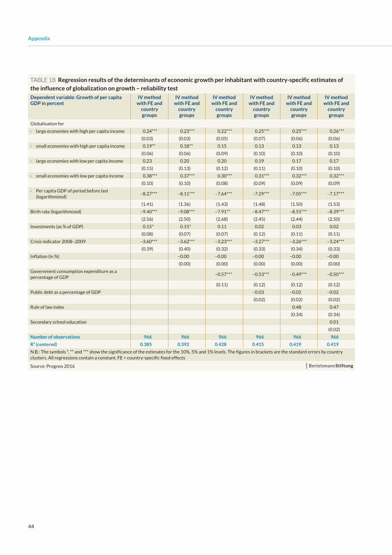
44
Appendix
Table 18 Regression results of the determinants of economic growth per inhabitant with country-specific estimates of
the influence of globalization on growth – reliability test
Dependent variable: Growth of per capita GDP in percent
IV method with FE and
country groups
IV method with FE and
country groups
IV method with FE and
country groups
IV method with FE and
country groups
IV method with FE and
country groups
IV method with FE and
country groups
Globalisation for
· large economies with high per capita income 0.24*** 0.23*** 0.22*** 0.25*** 0.25*** 0.26***
(0.03) (0.03) (0.05) (0.07) (0.06) (0.06)
· small economies with high per capita income 0.19** 0.18** 0.15 0.13 0.13 0.13
(0.06) (0.06) (0.09) (0.10) (0.10) (0.10)
· large economies with low per capita income 0.23 0.20 0.20 0.19 0.17 0.17
(0.15) (0.13) (0.12) (0.11) (0.10) (0.10)
· small economies with low per capita income 0.38*** 0.37*** 0.30*** 0.31*** 0.32*** 0.32***
(0.10) (0.10) (0.08) (0.09) (0.09) (0.09)
· Per capita GDP of period before last (logarithmized)
–8.27*** –8.11*** –7.64*** –7.29*** –7.05*** –7.17***
(1.41) (1.36) (1.43) (1.48) (1.50) (1.53)
Birth rate (logarithmized) –9.40*** –9.08*** –7.91** –8.47*** –8.55*** –8.39***
(2.56) (2.50) (2.68) (2.45) (2.44) (2.50)
Investments (as % of GDP) 0.15* 0.15* 0.11 0.02 0.03 0.02
(0.08) (0.07) (0.07) (0.12) (0.11) (0.11)
Crisis indicator 2008–2009 –3.60*** –3.62*** –3.23*** –3.27*** –3.26*** –3.24***
(0.39) (0.40) (0.32) (0.33) (0.34) (0.33)
Inflation (in %) –0.00 –0.00 –0.00 –0.00 –0.00
(0.00) (0.00) (0.00) (0.00) (0.00)
Government consumption expenditure as a percentage of GDP
–0.57*** –0.53*** –0.49*** –0.50***
(0.11) (0.12) (0.12) (0.12)
Public debt as a percentage of GDP –0.03 –0.02 –0.02
(0.02) (0.02) (0.02)
Rule of law index 0.48 0.47
(0.34) (0.34)
Secondary school education 0.01
(0.02)
Number of observations 966 966 966 966 966 966
R² (centered) 0.385 0.392 0.428 0.415 0.419 0.419
N.B.: The symbols *, ** and *** show the significance of the estimates for the 10%, 5% and 1% levels. The figures in brackets are the standard errors by country clusters. All regressions contain a constant. FE = country-specific fixed effects
Source: Prognos 2016

45
Appendix
Table 19 Absolute increase in globalization-induced per capita GDP 1990–2014 compared to the
overall increase in per capita GDP
Ranking Country Absolute increase in per capita GDP due to increasing
globalization, in euros*
Total absolute increase in per capita GDP, in euros*
Proportion of increase in per capita GDP due to increasing
globalization, in %
1 Japan 2,490 7,660 32.4
2 Ireland 1,600 19,430 8.2
3 Finland 1,550 7,590 20.5
4 Switzerland 1,520 7,250 20.9
5 Israel 1,350 12,400 10.9
6 Denmark 1,270 7,620 16.7
7 South Korea 1,320 13,480 9.8
8 Germany 1,160 8,460 13.7
9 Slovenia 1,050 4,630 22.7
10 Austria 1,020 8,830 11.5
11 Australia 960 9,790 9.9
12 Portugal 870 2,820 31.0
13 Greece 880 1,670 52.7
14 Sweden 810 11,350 7.2
15 Czech Republic 400 2,750 14.6
16 France 720 5,470 13.2
17 Canada 700 8,130 8.6
18 Netherlands 630 8,970 7.0
19 Estonia 690 2,640 26.0
20 Italy 680 1,390 49.3
21 Hungary 620 1,910 32.7
22 Slovakia 610 4,700 12.9
23 New Zealand 590 4,950 12.0
24 Lithuania 580 3,040 19.2
25 Spain 550 4,040 13.7
26 United Kingdom 510 10,620 4.8
27 Poland 520 4,620 11.3
28 Latvia 510 2,900 17.4
29 Norway 540 14,630 3.7
30 Chile 470 4,860 9.7
31 United States 430 12,970 3.3
32 Romania 360 1,400 26.0
33 Bulgaria 340 1,380 24.3
34 Belgium 330 7,120 4.7
35 South Africa 320 710 44.6
36 Turkey 280 2,890 9.7
37 Russia 220 580 37.8
38 Mexico 200 1,820 11.1
39 Brazil 190 1,730 11.2
40 China 180 3,130 5.8
41 India 40 710 5.9
42 Argentina 50 5,780 0.9
* actual prices in 2000; rounded values
Source: Prognos 2016

46
Appendix
Table 20 Relative increase in globalization-induced per capita GDP 1990–2014 compared to the
overall increase in per capita GDP
Ranking Country Increase in per capita GDP due to increasing
globalization compared to starting level, in %
Total increase in per capita GDP due to increasing
globalization compared to starting level, in %
Proportion of increase in per capita GDP due to increasing
globalization compared to starting level, in %
1 China 42,6 731,0 5,8
2 Bulgaria 18,5 76,2 24,3
3 Romania 18,4 70,8 26,0
4 South Korea 17,5 178,2 9,8
5 Poland 15,4 136,5 11,3
6 Estonia 13,6 52,3 26,0
7 Chile 13,4 137,8 9,7
8 Hungary 13,0 39,7 32,7
9 Lithuania 12,6 65,3 19,2
10 India 12,2 206,7 5,9
11 Latvia 11,4 65,7 17,4
12 Slovenia 11,3 49,8 22,7
13 Slovakia 11,0 85,4 12,9
14 Ireland 10,5 127,5 8,2
15 Portugal 9,0 29,1 31,0
16 South Africa 9,0 20,1 44,6
17 Israel 8,9 81,8 10,9
18 Greece 8,0 15,2 52,7
19 Russia 7,7 20,4 37,8
20 Turkey 7,4 76,8 9,7
21 Finland 7,1 34,7 20,5
22 Japan 6,7 20,6 32,4
23 Czech Republic 6,5 44,7 14,6
24 Germany 5,3 38,6 13,7
25 Brazil 5,2 47,0 11,2
26 Australia 5,1 51,3 9,9
27 Denmark 4,8 28,6 16,7
28 Austria 4,7 41,1 11,5
29 New Zealand 4,7 38,9 12,0
30 Spain 4,4 31,9 13,7
31 Switzerland 3,9 18,6 20,9
32 Italy 3,7 7,5 49,3
33 France 3,5 26,5 13,2
34 Mexico 3,3 29,9 11,1
35 Canada 3,2 37,3 8,6
36 Sweden 3,0 42,5 7,2
37 Netherlands 2,9 41,4 7,0
38 United Kingdom 2,2 46,8 4,8
39 Norway 1,8 47,8 3,7
40 Belgium 1,6 34,2 4,7
41 United States 1,3 40,6 3,3
42 Argentina 0,8 95,6 0,9
Source: Prognos 2016

47
Appendix
Table 21 Classification of economies investigated using per capita GDP and size of economy
Large economies with high per capita income
Small economies with high per capita income
Large economies with low per capita income
Small economies with low per capita income
Australia Belgium Argentina Bulgaria
Germany Denmark Brazil Chile
France Finland China Estonia
Italy Greece India Latvia
Japan Ireland Mexico Lithuania
Canada Israel Poland Romania
Netherlands New Zealand Portugal Slovakia
Switzerland Norway Russia Slovenia
Spain Austria South Africa Czech Republic
United States Sweden South Korea Hungary
United Kingdom Turkey
Source: Prognos 2016

48
Appendix
5.3 Additional Figures
FIGURE 13 Per capita GDP with and without globalization from 1990 to 2014, Argentina to France, in euros (baseline year 2000)
Source: Prognos 2016
per capita GDP without globalizationper capita GDP
Argentina
6,000
8,000
10,000
12,000
201420102005200019951990
3,500
4,000
4,500
5,000
5,500
201420102005200019951990
0
1,000
2,000
3,000
4,000
201420102005200019951990
3,000
4,000
5,000
6,000
7,000
8,000
201420102005200019951990
18,000
20,000
22,000
24,000
26,000
28,000
30,000
201420102005200019951990
1,500
2,000
2,500
3,000
3,500
201420102005200019951990
26,000
28,000
30,000
32,000
34,000
36,000
201420102005200019951990
18,000
20,000
22,000
24,000
26,000
28,000
30,000
32,000
201420102005200019951990
20000
22,000
24,000
26,000
28,000
201420102005200019951990
3,000
4,000
5,000
6,000
7,000
8,000
9,000
201420102005200019951990
22,000
24,000
26,000
28,000
30,000
32,000
201420102005200019951990
20,000
22,000
24,000
26,000
28,000
201420102005200019951990
Australia Belgium
Brazil Bulgaria Chile
China Denmark Germany
Estonia Finland France

49
Appendix
Source: Prognos 2016
per capita GDP without globalizationper capita GDP
FIGURE 14 Per capita GDP with and without globalization from 1990 to 2014, Greece to the Netherlands, in euros
(baseline year 2000)
Greece
10,000
12,000
14,000
16,000
18,000
201420102005200019951990
15,000
20,000
25,000
30,000
201420102005200019951990
20,000
22,000
24,000
26,000
28,000
30,000
201420102005200019951990
6,000
6,500
7,000
7,500
8,000
201420102005200019951990
200
400
600
800
1,000
1,200
201420102005200019951990
18,000
19,000
20,000
21,000
22,000
23,000
201420102005200019951990
2,000
3,000
4,000
5,000
6,000
7,000
8,000
201420102005200019951990
12,000
14,000
16,000
18,000
201420102005200019951990
15,000
20,000
25,000
30,000
35,000
201420102005200019951990
38,000
40,000
42,000
44,000
46,000
201420102005200019951990
2,000
3,000
4,000
5,000
6,000
7,000
8,000
201420102005200019951990
20,000
22,000
24,000
26,000
28,000
30,000
32,000
201420102005200019951990
India Ireland
Israel Italy Japan
Canada Latvia Lithuania
Mexico New Zealand Netherlands
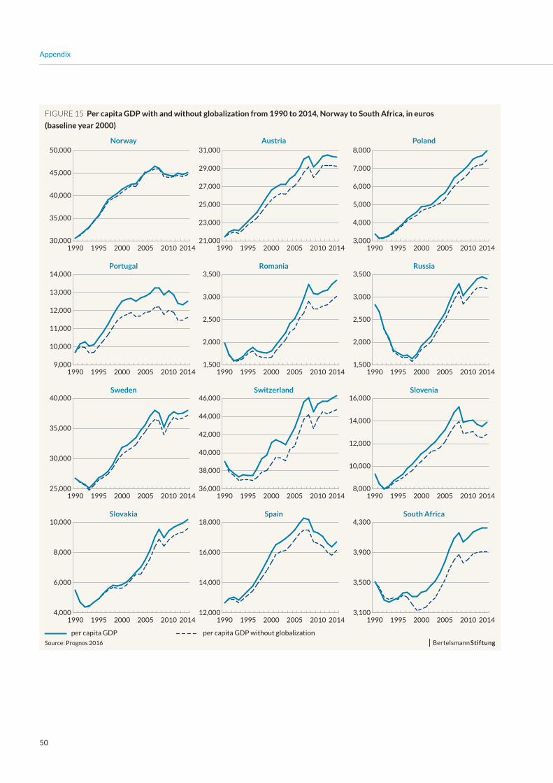
50
Appendix
Source: Prognos 2016
per capita GDP without globalizationper capita GDP
FIGURE 15 Per capita GDP with and without globalization from 1990 to 2014, Norway to South Africa, in euros
(baseline year 2000)
Norway
30,000
35,000
40,000
45,000
50,000
201420102005200019951990
9,000
10,000
11,000
12,000
13,000
14,000
201420102005200019951990
25,000
30,000
35,000
40,000
201420102005200019951990
4,000
6,000
8,000
10,000
201420102005200019951990
21,000
23,000
25,000
27,000
29,000
31,000
201420102005200019951990
1,500
2,000
2,500
3,000
3,500
201420102005200019951990
36,000
38,000
40,000
42,000
44,000
46,000
201420102005200019951990
12,000
14,000
16,000
18,000
201420102005200019951990
3,000
4,000
5,000
6,000
7,000
8,000
201420102005200019951990
1,500
2,000
2,500
3,000
3,500
201420102005200019951990
8,000
10,000
12,000
14,000
16,000
201420102005200019951990
3,100
3,500
3,900
4,300
201420102005200019951990
Austria Poland
Portugal Romania Russia
Sweden Switzerland Slovenia
Slovakia Spain South Africa

51
Appendix
Source: Prognos 2016
per capita GDP without globalizationper capita GDP
FIGURE 16 Per capita GDP with and without globalization from 1990 to 2014, South Korea to the United Kingdom, in euros
(baseline year 2000)
South Korea
6,000
10,000
14,000
18,000
22,000
201420102005200019951990
4,000
5,000
6,000
7,000
201420102005200019951990
5,000
6,000
7,000
8,000
9,000
201420102005200019951990
30,000
35,000
40,000
45,000
201420102005200019951990
3,000
4,000
5,000
6,000
7,000
201420102005200019951990
20,000
25,000
30,000
35,000
201420102005200019951990
Czech Republic Turkey
Hungary United States United Kingdom

52
Figures
Figure 1 Developments in the globalization index for selected countries for the period 1990–2014 12
Figure 2 Schematic representation of the change in gross domestic product and
globalization-induced income gains 15
Figure 3 Proportion of global exports supplied by country groups in %, 1995 to 2014 21
Figure 4 Change in exports and global market share, emerging countries, 1995 to 2014 23
Figure 5 Change in exports and global market share, Central and Eastern European countries,
1995 to 2014 24
Figure 6 Change in exports and global market share, large industrialized countries, 1995 to 2014 24
Figure 7 Change in exports and global market share, small industrialized countries, 1995 to 2014 25
Figure 8 Share of regions in global exports by sector, 1995 (upper bar) and 2014 (lower bar), in % 26
Figure 9 Share of German industrial goods exports by sector, 1995 and 2014, in % 27
Figure 10 Changes in global market shares of top ten exporters in automobile construction,
mechanical engineering and the chemical industry, 1995–2014 in % 28
Figure 11 Changes in global market shares of top ten exporters in office equipment and computers,
broadcasting and communication technology and rail transport construction sectors,
1995–2014 in % 29
Figure 12 Change in global market share and contribution of competitiveness to this change,
1995 to 2013, in % 32
Figure 13 Per capita GDP with and without globalization from 1990 to 2014, Argentina
to France, in euros (baseline year 2000) 48
Figure 14 Per capita GDP with and without globalization from 1990 to 2014, Greece
to the Netherlands, in euros (baseline year 2000) 49
Figure 15 Per capita GDP with and without globalization from 1990 to 2014, Norway
to South Africa, in euros (baseline year 2000) 50
Figure 16 Per capita GDP with and without globalization from 1990 to 2014, South Korea
to the United Kingdom, in euros (baseline year 2000) 51
Figures and Tables

53
Figures and Tables
Tables
Table 1 Globalization index for 2014 9
Table 2 Sub-indices of the globalization index for 2014 10
Table 3 Regression results of the determinants of economic growth per inhabitant 13
Table 4 Absolute per capita income gains due to increasing globalization 1990–2014 16
Table 5 Per capita income gains due to increasing globalization 1990-2014, weighted for
purchasing power 17
Table 6 Globalization-induced per capita income gains 1990-2014 compared to per capita
GDP in 1990 19
Table 7 Average and cumulative globalization-induced income gains at the national level
between 1990 and 2014 20
Table 8 Change in exports and global export market shares in 42 economies, 1995–2014, in% 22
Table 9 Portion of change in global market share due to increased/decreased competitiveness, in % 33
Table 10 Globalization indicators used 36
Table 11 Potential influences on economic growth as control variables for the regression analyses 38
Table 12 Globalization index over time, Argentina to Germany 40
Table 13 Globalization index over time, Estonia to Japan 40
Table 14 Globalization index over time, Canada to Austria 41
Table 15 Globalization index over time, Poland to Slovenia 41
Table 16 Globalization index over time, Spain to the United Kingdom 42
Table 17 Regression results of the determinants of economic growth per inhabitant – reliability test 43
Table 18 Regression results of the determinants of economic growth per inhabitant with
country-specific estimates of the influence of globalization on growth – reliability test 44
Table 19 Absolute increase in globalization-induced per capita GDP 1990–2014 compared to
the overall increase in per capita GDP 45
Table 20 Relative increase in globalization-induced per capita GDP 1990–2014 compared to
the overall increase in per capita GDP 46
Table 21 Classification of economies investigated using per capita GDP and size of economy 47
53

54
© 2016 Bertelsmann StiftungBertelsmann Stiftung
Carl-Bertelsmann-Straße 256
33311 Gütersloh
Phone +49 5241 81-0
www.bertelsmann-stiftung.de
ResponsibleDr. Thieß Petersen
AuthorsDr. Michael Böhmer,
Dr. Claudia Funke,
Dr. Andreas Sachs,
Heidrun Weinelt,
Johann Weiß,
Prognos AG, München
TranslationETC Europe scri
Grafic DesignNicole Meyerholz, Bielefeld
PictureMy Life Graphic | Shutterstock Images
PrintHans Kock Buch- und Offsetdruck, Bielefeld
Imprint


Adresse | Kontakt
Bertelsmann Stiftung
Carl-Bertelsmann-Straße 256
33311 Gütersloh
Phone +49 5241 81-0
Dr. Thieß Petersen
Programm Nachhaltig Wirtschaften
Phone +49 5241 81-81218
www.bertelsmann-stiftung.de