gmdh algorithm for modeling the outlet temperatures of a

Mechanics & Industry 18, 216 (2017)c© AFM, EDP Sciences 2017DOI: 10.1051/meca/2016034www.mechanics-industry.org

Mechanics&Industry

GMDH algorithm for modeling the outlet temperaturesof a solar chimney based on the ambient temperature

Alibakhsh Kasaeian1, Mehran Ghalamchi1, Mohammad Hossein Ahmadi1,a

and Mehrdad Ghalamchi2

1 Department of Renewable Energies, Faculty of New Science and Technologies, University of Tehran, Tehran, Iran2 Department of Energy Engineering, Graduate School of the Environment and Energy, Science and Research Branch,

Islamic Azad University, Tehran, Iran

Received 26 January 2016, Accepted 3 June 2016

Abstract – This work was carried out based on a constructed solar chimney with 2 m height and 3 m diam-eter. The temperature distributions were assessed based on the practical climatic conditions. In this work,the experimental data of temperature were investigated by a group method of data handling (GMDH).This method was applied as an artificial intelligence approach to predict the temperature changes, and alsoto find out the quality of the experimental data and temperature. In this case, a data set of 2000 condition-parameters for 30 days operation of solar chimney was applied. In order to obtain the network input andoutput variables, eight and four temperature sensors were set, respectively. In this study, according tothe value correlation coefficient (R2) and the root-mean square error (RMSE), the results of the trainednetworks have been reported. In the modeling and calculations, the ambient temperatures have been con-sidered. Also temperature prediction was carried out with high accuracy. Finally, the results showed thatthe solar chimney’s experimental data were qualified with no noise and some formulas were obtained foreach output based on the temperature input variables.

Key words: Solar chimney / temperature prediction / ambient temperature / GMDH method / neuralnetwork

1 Introduction

Renewable energy technologies are the clean sourcesof energy that have a much lower environmental impactthan conventional energy technologies. Among the renew-able sources, solar energy has a special situation in aspectsof accessibility and diversity. Solar chimney is one of themost popular types of energy production means in thesolar energy conversion area. The overall performance ofsolar chimney is described by some works which presentedresults for a prototype power plant built in Manzanares,Spain in 1982 [1–3]. Gannon and Von Backstrom [4] pre-sented an analytical model for a single rotor layout for alarge-scale solar chimney. The results show that the in-let guide vanes improve the performance. Also in anotherstudy [5] various radial sections were analyzed along theblades in the turbine model.

a Corresponding author:[email protected]

Bernardes et al. [6] proposed a thermal and techni-cal analysis for solar chimney power system. Bilgen andRheault [7] designed a solar chimney system for powerproduction at high latitudes and investigated its perfor-mance. The results showed solar chimney power plants athigh latitudes produce as much as 85% of the same plantsin the southern locations. Pretorius and Kroger [8] eval-uated the influence of convective heat transfer governingequations of solar chimney. Also that research aimed atappraising the effectiveness of different kinds of soil andquality of collector roof glass on the performance of aconventional solar chimney power plant.

Koonsrisuk and Chitsomboon [9] worked on dimen-sional analysis of solar chimney power plant and proposeddimensionless variables with computational fluid dynam-ics (CFD) method to compare the experimental study offlow in a small-scale solar chimney and in another re-search [10], they combined eight primitive variables toreach only one dimensionless variable. Zhou et al. [11] con-structed a small research pilot in which the temperature

Article published by EDP Sciences

https://doi.org/10.1051/meca/2016034

http://www.mechanics-industry.org

http://www.edpsciences.org

A. Kasaeian et al.: Mechanics & Industry 18, 216 (2017)

Nomenclature

cp Specific heat capacity (J.kg−1.K−1)

h Convective heat transfer coefficient (W.m−2.K−1)

m Mass flow rate (kg.s−1)

P Pressure (bar)

T Temperature (K)

V Quantity of velocity vector (m.s−1)

ρ Density (kg.m−3)

η Efficiency

Q Heat flow (kW)

g Gravitational acceleration (m.s−2)

H Chimney height (m)

Z Height (m)

q Heat flux (W.m−2)

D Diameter (m)

A Area of surface (m2)

r Collector radius (m)

f Friction coefficien

L Length (m)

Subscripts

a Ambient

A Absorber

co Collector

ch Chimney

t Turbine

difference between collector outlet and ambient reachedto 24.1 ◦C. Their results showed air temperature inver-sion appears in the chimney after sunrise both on a coolday and on a warm day.

Cost models for large-scale solar chimney power plantswere evaluated by Fluri et al. [12]. Thermodynamicmodeling of solar chimney power plant is studied byPetela [13], which was accompanied with evaluating en-ergy and exergy balances. The optimal chimney height formaximum power output was analyzed by Zhou et al. [14]and their results were validated with the measurementsof the prototype in Manzanares. Koonsrisuk et al. [15]described the constructed-theory for the geometry of so-lar chimney. Their results include an estimate of theheight/radius ratio, maximum power and maximum massflow rate. Bernardes and Backstrom [16] carried out somenumerical simulations to study the performance of solarchimney. They evaluated the flow volume and the turbinepressure drop in their model. Their results showed the op-timum ratio is not constant during the whole day and itis dependent on the heat transfer coefficients applied tothe collector. Chergui et al. [17] analyzed a natural lami-nar convective heat transfer problem in a solar chimney.Their analysis included the heat transfer process and thefluid flow in the collector and chimney.

Xu et al. [18] carried out numerical simulations on airflow, heat transfer and power output characteristics ofthe solar chimney power plant. This model included en-ergy storage layer and turbine which was similar to theManzanares prototype. They also proposed mathemati-

cal model of flow and heat transfer for the solar chim-ney power plant system. A new design of solar chimney-driven solar crop dryer (CDSCD) was presented by Afriyieet al. [19]. In another study [20], they developed mathe-matical models and a computer code to simulate the ven-tilation related to the design of the CDSCD.

Cao et al. [21] designed a sloped solar chimney powerplant, consisted of an air collector 607.2 m diameter and252.2 m chimney height. Their model was designed toproduce 5 MW electric power on a monthly average andafter that Koonsrisuk [22] presented mathematical mod-eling of sloped solar chimney power plants. Cao et al. [23]compared the performance of a conventional solar chim-ney power plant and sloped solar chimney based on a heattransfer model. Zuo et al. [24] presented a new solar chim-ney power system consisting sea water desalination thathad two usages, the production of electricity and fresh wa-ter. An exhaustive theoretical model for the performanceevaluation of a solar chimney power plant was proposedby Li et al. [25] and the results were verified by the experi-mental data of the Manzanares pilot. They also evaluatedthe effects of chimney height and collector radius on thepower output of a solar chimney. Hamdan [26] presenteda mathematical thermal model for steady state airflow in-side a solar chimney power plant based on Bernoulli equa-tion with buoyancy effect and ideal gas equation. Thatstudy showed that the optimum turbine head plays themost important role in productivity.

Several studies have been done in GMDH method andneural network for engineering fields. System identifica-tion techniques are utilized in various fields to model andpredict the behaviors of unknown and complex systemsbased on given input-output data [29]. For this purpose,soft computing methods, which involve computation in animprecise environment, have attracted considerable atten-tion of researchers. The components of fuzzy logic, neuralnetwork and evolutionary algorithms have great capabil-ity in solving complicated non-linear system identificationand control problems [30].

Many analytical studies have been expended to useevolutionary methods as applicable tools for systemidentification [31–33]. Among these methods, the groupmethod of data handling (GMDH) algorithm is a self-organizing approach which is generated based on the eval-uation of their performances on a set of multi-input andsingle output data pairs (Xi, Y i) (i = 1, 2, . . . , M). TheGMDH was introduced by Ivakhnenko [34] as a multi-variate analysis method for complicated systems model-ing and identification. In this way, the GMDH can be ap-plied to model complex systems without having specificknowledge of the systems.

The GMDH works by creating an analytical functionin a feed forward network based on a quadratic nodetransfer function in which coefficients are obtained byregression technique [35]. Actually, the real GMDH al-gorithm in which the model coefficients are approximatedby means of the least square method has been categorizedas complete induction and incomplete induction, which

18-page 2


represent the combinatorial (COMBI) and multi-layerediterative algorithms (MIA), respectively [36].

Recently, many researches were carried out based onstochastic search algorithms such as evolutionary meth-ods. In those studies, evolutionary methods were benefi-cial dealing with complex problems and were utilized todesign artificial neural networks. So the use of such self-organizing networks has result in successful application ofthe GMDH type algorithm in an extensive range of engi-neering, science and economics [37–43]. A comprehensivereview of utilizing evolutionary algorithms in the designof artificial neural networks is presented in [44]. In re-cent years, genetic algorithms have been employed in afeed forward GMDH type neural network for each neuronsearching its optimal set of connection with the precedinglayer [45].

In this study, GMDH method as great optimizing al-gorithm is suggested to forecast the output temperaturesof the solar chimney and implemented to decide on theinitial weights of the factors employed in neural network.In current work, 2000 pattern numbers, which have beengained from experimental device, are used for both train-ing the polynomial neural network according to R2 andRMSE and prediction output data

2 Theoretical analysis

2.1 Mathematical model of the solar chimney

To determine the mathematical model of the solarchimney, the governing equations for the movement ofair within the chimney and collector were considered sep-arately. The analysis of the solar chimney power plantis based on a mathematical model developed by Schlaichet al. and Munson [3,26–28]. A schematic diagram of thesolar chimney power plant is shown in Figure 1. Only the“simple” theoretical models are used to describe the en-tire power plant including the three major components,which are the solar collector, the chimney, and the windturbine.

Air is heated by solar radiation under a circular roofopen at the periphery. Since hot air is less dense than coldair, it rises up the chimney and is driven by the buoyancyeffect due to the vertical column of hot air. The fluid isassumed as an ideal gas and the air movement inside achimney is supposed to be a frictionless adiabatic pro-cess [26]. The system of the equations for an one dimen-sional steady compressible flow in a vertical chimney isexpressed as followings:

P3 − P4

gρ4= (z4 − z1)Gravity Head +

m2

2g(Achρ4)2

×(

fL

Dch+ Kin + Kout

)Friction Head

(1)

It is assumed that the distance between the ground andthe collector roof is considered large enough to disregardthe pressure drop in the collector section. So across the

Fig. 1. Schematic layout of a conventional solar chimneypower plant.

collector pressure drop is neglected; therefore the pressureat point 1 is equal to the pressure at point 2. So the massflow rate inside the solar chimney can be given by:

m = ρ3V3Ach (2)

According to reference [27], by balancing the kinetic andpotential energies of the flow, the speed of fluid at theinlet of chimney can be expressed as:

V3 =(

2ghchΔT

Ta

)(3)

An additional formula for the mass flow rate inside thesolar chimney using energy equation for the collector sec-tion is:

m =q′′Acoll

h2 − h1(4)

where q′′ is the heat flux and represents the absorbedsolar radiation excluding the thermal losses. The mainunknown in above equations is h2. Because the surfacearea of the collector is much larger than the surface areaof the chimney, it is assumed the heat radiated to thechimney is ignored. Therefore there is only a little tem-perature change across the chimney which is expressed asEquation (5).

T3 = T4 (5)

Entropy across the turbine is taken constant, hence thepressure expansion is assumed to be reversible and adi-abatic; therefore the entropy in point 3 is equal to theentropy in point 2. The pressure head is related to tur-bine head which is given by:

P3 = P2 − ρ2gHt (6)

2.2 Theoretical modeling of GMDH typeof Artificial Neural Network

The group method of data handling (GMDH) isa category of inductive algorithms for computer-based

18-page 3


mathematical modeling of multi-parametric datasets thatfeatures parametric optimization of models. The methodis a set of neurons in which various pairs of them ineach layer are connected through a quadratic polynomial,therefore, generate new neurons in the next layer. Thisexpression may be used in modeling to map inputs tooutputs. In fact, the formal definition includes a functionf in order to predict the output y for a specified inputvector X = (x1, x2, x3, . . . , xn). f and y are the actualinput and output which are defined as followings:

yi = f(xi1, xi2, xi3, . . . , xin) (i = 1, 2, 3, . . . , M) (7)

yi = f(xi1, xi2, xi3, . . . , xin) (i = 1, 2, 3, . . . , M) (8)

Then, a GMDH type neural network must be applied inorder to minimize the square of difference between theactual output and the predicted one:

M∑i=1

[f(xi1, xi2, xi3, . . . , xin) − yi

]2

→ min (9)

The connection between the input and output variablescan be expressed by a Kolmogorov-Gabor polynomial [34,36–38]:

y = a0 +n∑

i=1

aixi +n∑

i=1

n∑j=1

aijxixj

+n∑

i=1

n∑j=1

n∑k=1

aijkxixjxk + . . . (10)

y = G(xi, xj) = a0 + a1xi + a2xj + a3x2i + a4x

2j + a5xixj

(11)

In order to minimize the difference between the actualoutput, y, and the calculated one, y for each pair of xi, xj

as input variables, the coefficients ai in Equation (11) arecalculated by regression techniques.

In fact, a tree of polynomials is built using thequadratic form provided in Equation (11) whose coeffi-cients are calculated in a least-squares sense. In this re-gard, the coefficients of each quadratic function Gi areobtained to optimally fit the output in the whole set ofinput–output data pair, as follows:

E =

M∑i

(yi − Gi)2

M→ min (12)

Simply, in the GMDH algorithm, all the possibilities oftwo independent variables out of total n input variablesare selected in order to construct the regression polyno-mial in the form of Equation (11) that best fits the depen-dent observations (yi, i = 1, 2, . . . , M) in a least-squaressense.

Actually,(

n2

)=

n(n − 1)2

neurons will be

consequently built up in the first hidden layerof the feed forward network from the observa-tions {(yi, xip, xiq); (i = 1, 2, . . . , M} for different p, q ∈

Fig. 2. A generalized GMDH network structure of chromo-some.

{1, 2, . . . , n}. In other words, it is now possible to con-struct Mdata triples{(yi, xip, xiq); (i = 1, 2, . . . , M} fromthe observation using such p, q ∈ {1, 2, . . . , n} in the formof ⎡

⎣x1p x1q y1

x2p x2q y2

x3p x3q yM

⎤⎦

Using the quadratic sub-expression in the form of Equa-tion (11) for each row of M data triples, the followingmatrix equation can be readily obtained as

Aa = Y (13)a = {a0, a1, a2, a3, a4, a5} (14)

Y = {y1, y2, y3, . . . , yM}T (15)

where a is the vector of unknown coefficients for thequadratic polynomial in Equation (11), and Y is the vec-tor of output values from observation. A is given by:

A =

⎡⎣1 x1p x1q x1px1q x2

1p x21q

1 x2p x2q x2px2q x22p x2

2q

1 xMp xMq xMpxMq x2Mp x2

Mq

⎤⎦ (16)

The least-squares technique from multiple-regression re-sult is expressed as:

a =(AT A

)−1AT (17)

Point to note that this procedure for each neuron of thenext hidden layer is iterated and neurons in each layerare only connected to the neuron in its adjoining layer.Such a solution from normal equations is directly rathersusceptible to round off errors [44–49].

Taking this advantage, it was possible to perform asimple encoding scheme for the genotype of each individ-ual in the population as already proposed by [42–45]. Theencoding schemes are shown in Figure 2.

According to Figure 2, output neuron (abbcadad) in-cludes twice ad because the neuron (ad) at the first layer isconnected to the output layer by directly going throughthe second layer. This procedure occurs when a neuronpasses some adjoining hidden layers and connects to an-other neuron in the next following hidden layer. In thismethod scheme, the number of repetitions of neuron wasgiven by 2n where n is the number of the passed hid-den layers. The natural roulette wheel selection method

18-page 4


is applied to choose two parents for producing two off-spring’s [42–45].

Combining of genetic algorithm with the GMDH typeneural networks is started with representing each networkas a string of the concatenated sub-strings of alphabeticaldigits. The fitness, ϕ, of each entire string of symbolic dig-its which represents a GMDH type neural network modelis evaluated as followings [50–52]:

φ =1E

(18)

where E is the mean square of error which is minimizedwithin the evolutionary process by maximizing the fitness,ϕ. In this step, GMDH type neural network methods areproduced by progressively increasing fitness, ϕ, until nofurther substantial progress is possible.

These statistical fields are based on RMSE as the root-mean squared error, R2 as the absolute fraction of vari-ance, and MAPE as the mean absolute percentage of errorwhich are given by [50–52]:

R2 = 1 −[∑M

i=0

(Yi(model) − Yi(Actual)

)2

∑Mi=1

(Yi(Actual)

)2

](19)

RMSE =

[∑Mi=0

(Yi(model) − Yi(Actual)

)2

M

]1/2

(20)

MAPE =

[∑Mi=0

∣∣Yi(model) − Yi(Actual)

∣∣M

∑Mi=1

(Yi(Actual)

)]

(21)

3 Results and discussion

An experimental solar chimney pilot consisted of anair collector 3 m in diameter and chimney height of 2 mwas constructed at University of Tehran, Iran. The tem-perature distribution in the solar chimney setup was mea-sured by 12 SMT160 sensors and recorded on data-loggersetup. Eight of these sensors were utilized as the inputsof the system and four sensors as the outputs. The ar-rangement of the sensors is shown in Figure 3. As it isobserved, six sensors are located on the absorbers, fourones are embedded for temperature measuring of the fluidand one sensor is put at the inlet of the chimney. T ′

1 to T ′8

indicate the system inputs while T1 to T4 represent thesystem outputs.

The GMDH-type neural networks have been used tofind the input-output relationship in the form of polyno-mial models. Such neural network identification processneeds, in turn, some optimization methods to find thebest network architecture. With this regard, GAs are or-ganized in a new approach to design the whole architec-ture of the GMDH-type neural networks, i.e., the numberof neurons in each hidden layer and their connectivityconfiguration combined with Singular Value Decomposi-tion (SVD). This combination is applied to discover theoptimal coefficients of quadratic expressions for modelingand prediction of the output temperatures based on theinput data of the constructed solar chimney.

Fig. 3. Sensor arrangement of the absorber and fluid.

Table 1. Amount of the absolute fraction of variance, theroot-mean squared error and the mean absolute percentagefor T1 model.

R2 0.9906MAPE 0.00000915RMSE 0.8027


R2 0.9875MAPE 0.00001032RMSE 0.9268


R2 0.9822MAPE 0.00001240RMSE 1.0664

Table 4. Amount of the absolute fraction of variance, theroot-mean squared error and the mean absolute percentagefor T4model.

R2 0.983MAPE 0.00001096RMSE 0.9728

Some statistical measures for T1, T2, T3 and T4 aregiven in Tables 1–4, respectively. The correlation coeffi-cient is high in all sections and this is shown that accuracyof the trained networks is appreciate.

The corresponding polynomial representation of sucha model for T1 is as followings:

See equation (22) next page.

The corresponding polynomial representation of such amodel for T2 is presented as:


The corresponding polynomial representation of such amodel for T3 is read as:


18-page 5


T1 = 0.649482 + N76 × 1.18442 − N76 × N48 × 0.0213749 − N48 × 0.225523 + N482 × 0.0219758

N48 = −13.4559 − 2.00866 × T ′3 + T ′

3 × N115 × 0.272208 − (T ′

3

)2 × 0.0875282 + N115 × 4.15735 − N1152 × 0.209706

N76 = −20.1938 + T ′2 × 3.02076 + T ′

2 × T ′6 × 0.0736612 − (

T ′2

)2 × 0.0893313 − T ′6 × 0.56505 − (

T ′6

)2 × 0.0129832

N115 = 2.82216 − T ′1 × 0.390159 + T ′

1 × T ′7 × 0.0203775 − (

T ′1

)2 × 0.00689403 + T ′7 × 1.23392 − (

T ′7

)2 × 0.0158294 (22)

T2 = 0.268754 + N46 × 0.281634 + N46 × N60 × 0.00839465 + N60 × 0.699729 − N602 × 0.00809195

N46 = −3.71305 + N90 × 3.13447 + N90 × N121 × 0.0646854 − N902 × 0.0673995 − N121 × 1.92171

N60 = −4.88004 + N86 × 0.317896 + N86 × N106 × 0.0506992 − N862 × 0.0207954 + N106 × 0.959815 − N1062 × 0.0335401

N86 = −42.2945 + T ′2 × 6.27282 + T ′

2 × T ′6 × 0.13522 − (

T ′2

)2 × 0.186239 − T ′6 × 1.80287 − (

T ′6

)2 × 0.0202776

N90 = −0.484459 + T ′4 × 1.42028 + T ′

4 × T ′7 × 0.225981 − (

T ′4

)2 × 0.13289 − T ′7 × 0.282354 − (

T ′7

)2 × 0.100004

N106 = −25.4119 − T ′1 × 1.12963 + T ′

1 × T ′2 × 0.0629554 − (

T ′1

)2 × 0.00194151 + T ′2 × 3.87368 − (

T ′2

)2 × 0.0907913

N121 = 22.4997 − T ′3 × 1.50276 − T ′

3 × T ′8 × 0.166964 +

(T ′

3

)2 × 0.118525 + T ′8 × 1.25398 +

(T ′

8

)2 × 0.0626675 (23)

T3 = −2.06804 + N92 × 2.21536 + N92 × N39 × 0.199213 − N922 × 0.139326 − N39 × 1.08793 − N392 × 0.0617369

N39 = −0.688241 + N70 × 0.583494 − N702 × 0.000499522 + N74 × 0.454862

N70 = −26.2777 + T ′2 × 3.76542 + T ′

2 × T ′3 × 0.0751355 − (

T ′2

)2 × 0.103888 − T ′3 × 0.732453 − (

T ′3

)2 × 0.0113413

N74 = −1.62996 + T ′2 × 2.08367 + T ′

2 × T ′6 × 0.0796999 − (

T ′2

)2 × 0.0761524 − T ′6 × 0.7946 − (

T ′6

)2 × 0.0130868

N92 = −42.6409 + T ′2 × 5.33236 + T ′

2 × T ′4 × 0.0773835 − (

T ′2

)2 × 0.133506 − T ′4 × 1.01139 − (

T ′4

)2 ∗ 0.00974921 (24)

Finally, the corresponding polynomial representation ofsuch a model for T4 is stated as:


As it is shown in Figure 4, the trained network is anacceptable network based on GMDH algorithm with R2

equal to 0.9906. Figure 5 shows the deviation of GMDHbased on network outputs from experimental data whichis acceptable 10 percent of experimental data. Figure 6shows that all data are of high quality and have verylow deviation. Also this figure shows excellent agreementbetween the achieved experimental data for T1 and theGMDH algorithm outputs

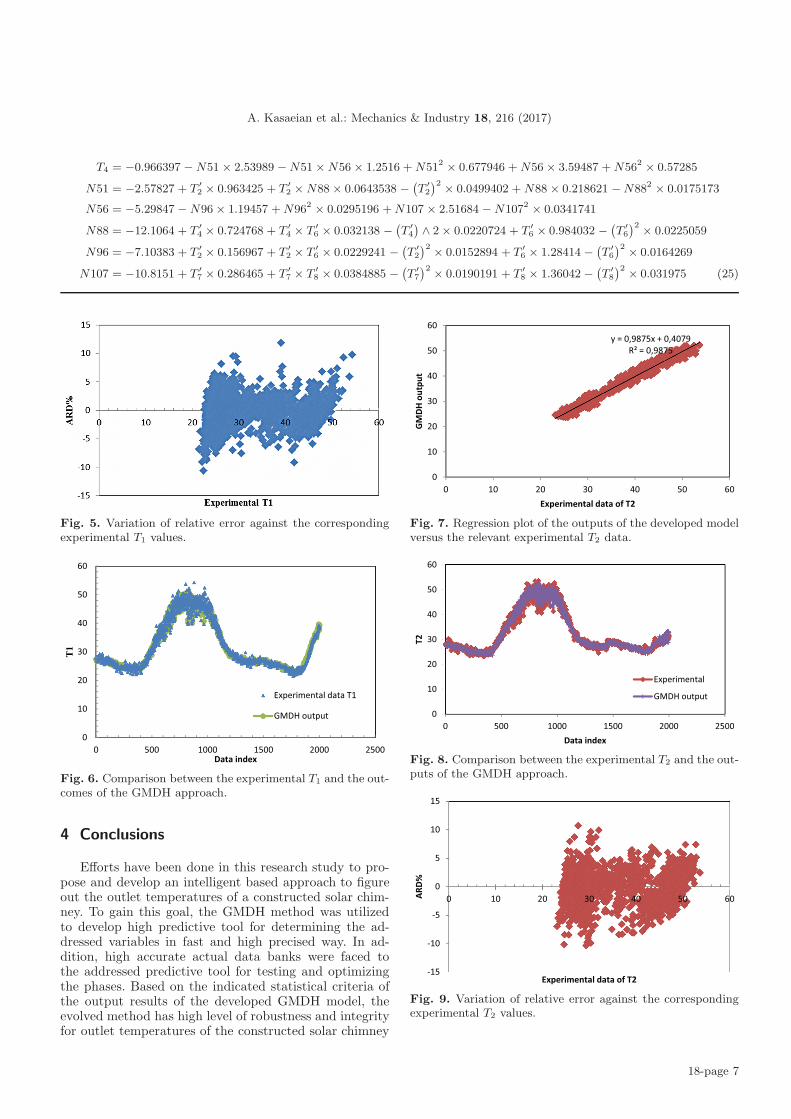
Comparison of the GMDH-based trained network datafor T2 and the T2 experimental data is shown in Figure 7.According to Figure 7, the trained networks based onGMDH have R2 equal to 0.9875, and this indicates thatthe networks have been trained from high quality experi-mental data of T2. A high agreement between the GMDHoutput data and the experimental data of T2is shown inFigure 8. Figure 9 shows the deviation of GMDH basedon the network results obtained of the experimental data.As it is evident, due to the high quality of the data, thereare deviations between –10% to +10% which is perfectlyacceptable.

In Figure 10, the output of the trained network basedon GMDH for T3 shows that R2 is 0.9822. Also Figure 11shows the GMDH output data and the experimental data

0

10

20

30

40

50

60

GM

DH

out

put

0

0

0

0

0

0

0

0 10 220 30

Experimenta

y = 0,99R²

0 40

al data of T1

906x + 0,2987 = 0,9906

50

7

60

Fig. 4. Regression plot of the outputs of the developed modelversus the relevant experimental T1 data.

of T3. The deviation of GMDH output data from experi-mental data of T3 is shown in Figure 12.

Figure 13 shows the quality of the trained networkbased on GMDH algorithm for T4 with R2 equal to 0.983.The deviation of GMDH output data from experimentaldata of T4 is shown in Figure 14. In Figure 15, the com-parison between the predicted data by GMDH algorithmfor T4 and the T4 experimental data is shown and a goodagreement is observed.

18-page 6


T4 = −0.966397 − N51 × 2.53989 − N51 × N56 × 1.2516 + N512 × 0.677946 + N56 × 3.59487 + N562 × 0.57285

N51 = −2.57827 + T ′2 × 0.963425 + T ′

2 × N88 × 0.0643538 − (T ′

2

)2 × 0.0499402 + N88 × 0.218621 − N882 × 0.0175173

N56 = −5.29847 − N96 × 1.19457 + N962 × 0.0295196 + N107 × 2.51684 − N1072 × 0.0341741

N88 = −12.1064 + T ′4 × 0.724768 + T ′

4 × T ′6 × 0.032138 − (

T ′4

) ∧ 2 × 0.0220724 + T ′6 × 0.984032 − (

T ′6

)2 × 0.0225059

N96 = −7.10383 + T ′2 × 0.156967 + T ′

2 × T ′6 × 0.0229241 − (

T ′2

)2 × 0.0152894 + T ′6 × 1.28414 − (

T ′6

)2 × 0.0164269

N107 = −10.8151 + T ′7 × 0.286465 + T ′

7 × T ′8 × 0.0384885 − (

T ′7

)2 × 0.0190191 + T ′8 × 1.36042 − (

T ′8

)2 × 0.031975 (25)

Fig. 5. Variation of relative error against the correspondingexperimental T1 values.

0

10

20

30

40

50

60

0 500 1000 1500 2000 2500

T1

Data index

Experimental data T1

GMDH output

Fig. 6. Comparison between the experimental T1 and the out-comes of the GMDH approach.

4 Conclusions

Efforts have been done in this research study to pro-pose and develop an intelligent based approach to figureout the outlet temperatures of a constructed solar chim-ney. To gain this goal, the GMDH method was utilizedto develop high predictive tool for determining the ad-dressed variables in fast and high precised way. In ad-dition, high accurate actual data banks were faced tothe addressed predictive tool for testing and optimizingthe phases. Based on the indicated statistical criteria ofthe output results of the developed GMDH model, theevolved method has high level of robustness and integrityfor outlet temperatures of the constructed solar chimney

y = 0,9875x + 0,4079R² = 0,9875

0

10

20

30

40

50

60

0 10 20 30 40 50 60

GM

DH

out

put

Experimental data of T2


0

10

20

30

40

50

60

0 500 1000 1500 2000 2500

T2

Data index

Experimental

GMDH output

Fig. 8. Comparison between the experimental T2 and the out-puts of the GMDH approach.

-15

-10

-5

0

5

10

15

0 10 20 30 40 50 60ARD

%



18-page 7


y = 0,9822x + 0,5811R² = 0,9822

0

10

20

30

40

50

60

0 10 20 30 40 50 60

GM

DH

out

put



0

10

20

30

40

50

60

0 500 1000 1500 2000 2500

T3

Data index

Experimental

GMDH output

Fig. 11. Comparison between the experimental T3 and theoutcomes of the GMDH approach.

-15

-10

-5

0

5

10

15

0 10 20 30 40 50 60ARD

%



determination. The last step of this study is shown thatthe output results of the GMDH approach could help en-ergy experts to design solar chimney with high level ofperformance, reliability and robustness and low degree ofuncertainty. The results show that the solar chimney’sexperimental data were qualified and according to mod-eling, the formulas of the outlet temperatures have beenobtained.

y = 0,983x + 0,5455R² = 0,983

0

10

20

30

40

50

0 10 20 30 40 50 60

GM

DH

out

put

Experimental data T4


-15

-10

-5

0

5

10

15

0 10 20 30 40 50 60ARD

%



0

10

20

30

40

50

60

0 500 1000 1500 2000 2500

T4

Data index

Experimental

GMDH output

Fig. 15. Comparison between the experimental T4 and theoutputs of the GMDH approac.

References

[1] W. Haaf, K. Friedrich, G. Mayr, J. Schlaich, Solar chim-neys, part I: principle and construction of the pilot plantin Manzanares, Int. J. Solar Energy 2 (1983) 3–20

[2] W. Haaf, Solar chimneys, part II: preliminary test resultsfrom the Manzanares pilot plant, Int. J. Solar Energy 2(1984) 141–161

[3] J. Schlaich, The Solar Chimney, Electricity from the Sun,Deutsche Verlags-Anstalt, Stuttgart, 1994

[4] A.J. Gannon, T.W. Von Backstrom, Controlling andmaximizing solar chimney power output, In: Proceedingsof the 1st International Conference on Heat Transfer,

18-page 8


Fluid Mechanics and Thermodynamics, Kruger Park,South Africa, 2002

[5] T.P. Fluri, T.W. Von Backstrom, Comparison of mod-elling approaches and layouts for solar chimney turbines,Solar Energy 82 (2008) 239–246

[6] M.A. Bernardes, D.S. Voß, G. Weinrebe, Thermal andtechnical analyses of solar chimneys, Solar Energy 75(2003) 511–524

[7] E. Bilgen, J. Rheault, Solar chimney power plants forhigh latitudes, Solar Energy 79 (2005) 449–458

[8] J.P. Pretorius, D.G. Kroger, Critical evaluation of so-lar chimney power plant performance, Solar Energy 80(2006) 535–544

[9] A. Koonsrisuk, T. Chitsomboon, Dynamic similarity insolar chimney modeling, Solar Energy 81 (2007) 1439–1446

[10] A. Koonsrisuk, T. Chitsomboon, A single dimensionlessvariable for solar chimney power plant modeling, SolarEnergy 83 (2009) 2136–2143

[11] X. Zhou, J. Yang, B. Xiao, G. Hou, Experimental study oftemperature field in a solar chimney power setup, Appl.Thermal Eng. 27 (2007) 2044–2050

[12] T.P. Fluri, J.P. Pretorius, C. Van Dyk, T.W. VonBackstrom, D.G. Kroger, G. Van Zijl, Cost analysis ofsolar chimney power plants, Solar Energy 83 (2009) 246–256

[13] R. Petela, Thermodynamic study of a simplified modelof the solar chimney power plant, Solar Energy 83 (2009)94–107

[14] X. Zhou, J. Yang, B. Xiao, G. Hou, F. Xing, Analysisof chimney height for solar chimney power plant, Appl.Thermal Eng. 29 (2009) 178–185

[15] A. Koonsrisuk, S. Lorente, A. Bejan, Constructal solarchimney configuration, Int. J. Heat Mass Transfer 53(2010) 327–333

[16] M. Bernardes, W. Theodor, T.W. Von Backstrom,Evaluation of operational control strategies applicable tosolar chimney power plants, Solar Energy 84 (2010) 277–288

[17] T. Chergui, S. Larbi, A. Bouhdjar, Thermo-hydrodynamic aspect analysis of flows in solar chimneypower plants-A case study, Renew. Sustain. Energy Rev.14 (2010) 1410–1418

[18] G. Xu, T. Ming, Y. Pan, F. Meng, C. Zhou, Numericalanalysis on the performance of solar chimney power plantsystem, Energy Convers. Manage. 52 (2011) 876–883

[19] J.K. Afriyie, M.A. Nazha, H. Rajakaruna, F.K. Forson,Experimental investigations of a chimney-dependent so-lar crop dryer, Renew. Energy 34 (2009) 217–222

[20] J.K. Afriyie, H. Rajakaruna, M.A. Nazha, F.K. Forson,Simulation and optimization of the ventilation in achimney-dependent solar crop dryer, Solar Energy 85(2011) 1560–1573

[21] F. Cao, L. Zhao, L. Guo, Simulation of a sloped so-lar chimney power plant in Lanzhou, Energy Convers.Manage. 52 (2011) 2360–2366

[22] A. Koonsrisuk, Mathematical modeling of sloped solarchimney power plants, Energy 47 (2012) 582–589

[23] F. Cao, L. Zhao, H. Li, L. Guo, Performance analysis ofconventional and sloped solar chimney power plants inChina, Appl. Thermal Eng. 50 (2013) 582–592

[24] L. Zuo, Y. Zheng, Z. Li, Y. Sha, Solar chimneys integratedwith sea water desalination, Desalination 276 (2011) 207–213

[25] J. Li, P. Guo, Y. Wang, Effects of collector radius andchimney height on power output of a solar chimney powerplant with turbines, Renew. Energy 47 (2012) 2128

[26] M. Hamdan, Analysis of solar chimney power plant uti-lizing chimney discrete model, Renew. Energy 56 (2013)50–54

[27] E. Sanchez, T. Shibata, L.A. Zadeh, Genetic algorithmsand fuzzy logic systems, World Scientific, River edge NJ,1997

[28] K. Kristinson, G. Dumont, System identification and con-trol using genetic algorithms, J. IEEE Trans. Syst. Man.Cybern 22 (1992) 1033–46

[29] J. Koza, Genetic programming, on the programming ofcomputers by means of natural selection, MIT Press, MA,Cambridge, 1992

[30] H. Iba, T. Kuita, deH. Garis, T. Sator, System identifica-tion using structured genetic algorithms, In: Proceedingsof the 5th international conference on genetic algorithms,ICGA’93, USA, 1993

[31] K. Rodrıguez-Vazquez, Multi-objective evolutionary al-gorithms in non-linear system identification, Ph.D.Thesis, University of Sheffield, Sheffield, UK, 1999

[32] A.G. Ivakhnenko, Polynomial Theory of ComplexSystems, IEEE Trans. Syst. Man Cybern SMC-1 (1971)364–378

[33] S.J. Farlow, Self-organizing method in modelling, GMDHtype algorithm, Marcel Dekker Inc., 1984

[34] J.A. Mueller, F. Lemke, Self-organizing data mining: anintelligent approach to extract knowledge from data, Pub.Libri, Hamburg, 2000

[35] N. Nariman-zadeh, A. Darvizeh, M.E. Felezi, H.Gharababei, Polynomial modeling of explosive com-paction process of metallic powders using GMDH-typeneural networks and singular value decomposition, J.Model Simul. Mater. Eng. 10 (2002) 727–44

[36] C.M. Fonseca, P.J. Fleming, Nonlinear system identifica-tion with multi-objective genetic algorithm proceedingsof the 13th World congress of the international federationof automatic control, Pergamon Press, San Francisco,California, 1996, pp. 187–92

[37] G.P. Liu, V. Kadirkamanathan, Multi-objective crite-ria for neural network structure selection and identifica-tion of nonlinear systems using genetic algorithms, IEEEProc. Control Theory Appl. 146 (1999) 373–82

[38] N. Nariman-Zadeh, A. Darvizeh, R. Ahmad-Zadeh,Hybrid Genetic Design of GMDH-Type Neural NetworksUsing Singular Value Decomposition for Modelling andPrediction of the Explosive Cutting Process, Proc. IMECH E Part B. J. Eng Manuf. 217 (2003) 779–790

18-page 9


[39] V.W. Porto, Evolutionary computation approaches tosolving problems in neural computation, In: Handbookof evolutionary computation, edited by Back D.B. Fogel,Michalewicz Z, Oxford University Press, Institute ofPhysics Publishing and New York, 1997, pp. D1.2, 1–6

[40] X. Yao, Evolving artificial neural networks, Proc. IEEE87 (1999) 1423–47

[41] E.F. Vasechkina, V.D. Yarin, Evolving polynomial neuralnetwork by means of genetic algorithm: some applicationexamples, Complex Int. 9 (2001)

[42] X. Yao, Evolving Artificial Neural Networks, Proc. IEEE87 (1999) 1423–1447

[43] N. Nariman-zadeh, K. Atashkari, A. Jamali, A. Pilechi,X. Yao, Inverse modelling of multi-objective thermody-namically optimized turbojet engines using GMDH-typeneural networks and evolutionary algorithms, J. Eng.Optim. 37 (2005) 43–62

[44] B.R. Munson, D.F. Young, T.O. Okiishi, Fundamentalsof fluid mechanics, 2nd edition, John Wiley & Sons, Inc,1994, Chap. 2

[45] J. Schlaich, R. Bergermann, W. Schiel, G. Weinrebe,Design of commercial solar updraft tower systems uti-lization of solar induced convective flows for power gen-eration, J. Solar Energy Eng. 127 (2005) 117–124

[46] K. Atashkari, Nariman-Zadeh, N, Jamali, A, Pilechi, A,Thermodynamic Pareto optimization of turbojet usingmulti-objective genetic algorithm, Int. J. Thermal Sci. 44(2005) 1061–1071

[47] K. Atashkari, N. Nariman-Zadeh, M. Golcu, A.Khalkhali, A. Jamali, Modelling and multi-objective opti-mization of a variable valve-timing spark- ignition engineusing polynomial neural networks and evolutionary algo-rithms, Energy Convers. Manage. 48 (2007) 1029–1041

[48] A. Jamali, N. Nariman-zadeh, A. Darvizeh, A. Masoumi,S. Hamrang, Multi- objective evolutionary optimizationof polynomial neural networks for modelling and predic-tion of explosive cutting process, Eng. Appl. Artif. Intell.22 (2009) 67–687

[49] J.I.E. Lin, C.T. Cheng, K.W. Chau, Using support vec-tor machines for long-term discharge prediction, Hydrolo.Sci. J. 51 (2006) 599–612

[50] M.H. Ahmadi, M.-A. Ahmadi, M. Mehrpooya, M.A.Rosen, Using GMDH Neural Networks to Model thePower and Torque of a Stirling Engine, Sustainability 7(2015) 2243–2255

[51] R. Shirmohammadi, B. Ghorbani, M. Hamedi, M.-H.Hamedi, L.M. Romeo, Optimization of mixed refriger-ant systems in low temperature applications by means ofgroup method of data handling (GMDH), J. Natural GasSci. Eng. 26 (2015) 303–312

[52] S.M. Pourkiaei, H.A. Mohammad, S. MahmoudHasheminejad, Modeling and experimental verificationof a 25W fabricated PEM fuel cell by parametric andGMDH-type neural network, Mech. Ind. 17 (2016) 105

18-page 10

gmdh algorithm for modeling the outlet temperatures of a

Documents