gmm

Seminar IV - GMMKrenar AvdulajOctober 27th, 2014

GMM estimation was formalized by Hansen (1982), and since has become one of the most widely usedmethods of estimation for models in economics and finance.

1. Unlike MLE, GMM does not require complete knowledge of the distribution of the data. Only specifiedmoments derived from an underlying model are needed for GMM estimation.

2. In some cases in which the distribution of the data is known, MLE can be computationally veryburdensome whereas GMM can be computationally very easy. (e.g. log-normal stochastic volatilitymodel.)

3. In models for which there are more moment conditions than model parameters, GMM estimationprovides a straightforward way to test the specification of the proposed model.

Single Equation Linear GMMShort reviewConsider the linear regression

where is a Lx1 vector of explanatory variables, a vector of unknown coefficients and is a randomerror term. Some of elements are possibly correlated with (possibly being endogenous variable). Inaddition assume is a vector of instrumental variables of size Kx1. Let represent the vector of uniqueand non-constant elements of .

Basic ideaGMM estimator of in exploits the orthogonality condition

The idea is to create a set of equations for by making sample moments match the population moments.

Sample moments:

Population moment

Sample moment=population moment

= + , t = 1,… , nyt z′t δ0 ϵt

zt δ0 ϵtzt ϵt

xt wt{ , , }yt zt xt

δ = +yt z′t δ0 ϵt

E[ ( , )] = E[ ] = E[ ( + )] = 0gt wt δ0 xtϵt xt yt z′t δ0

δ

(δ)gn = g( , δ) = (y + δ))1n ∑

t=1

n

wt1n ∑

t=1

n

xt z′t

= ⇒ K set of equations with L unknowns

⎛

⎝

⎜⎜⎜

(y + δ)1n *

nt=1 x1t z′

t

⋮

(y + δ)1n *

nt=1 xKt z′

t

⎞

⎠

⎟⎟⎟

E[ ] = 0xtϵt

n n

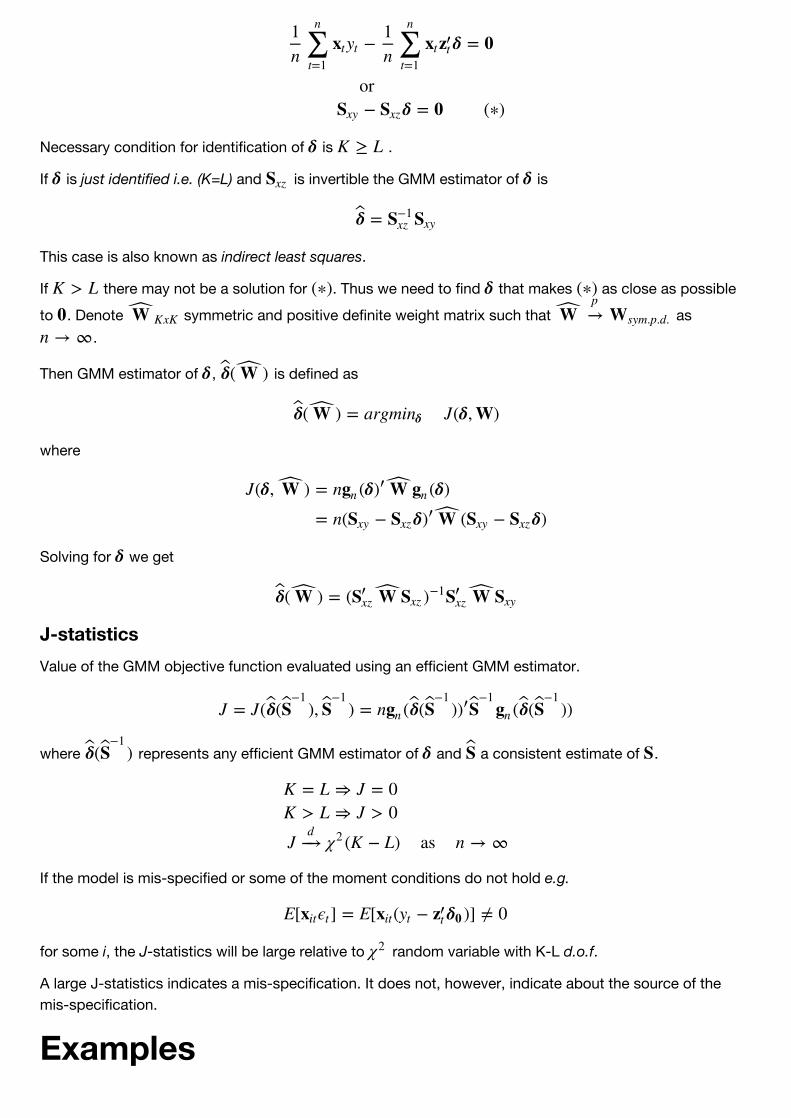
Necessary condition for identification of is .

If is just identified i.e. (K=L) and is invertible the GMM estimator of is

This case is also known as indirect least squares.

If there may not be a solution for . Thus we need to find that makes as close as possible

to . Denote symmetric and positive definite weight matrix such that as .

Then GMM estimator of , is defined as

where

Solving for we get

J-statisticsValue of the GMM objective function evaluated using an efficient GMM estimator.

where represents any efficient GMM estimator of and a consistent estimate of .

If the model is mis-specified or some of the moment conditions do not hold e.g.

for some i, the J-statistics will be large relative to random variable with K-L d.o.f.

A large J-statistics indicates a mis-specification. It does not, however, indicate about the source of themis-specification.

Examples

1n ∑

t=1

n

xtyt

Sxy

+ δ = 01n ∑

t=1

n

xtz′t

or+ δ = 0 (0)Sxz

δ K ~ L

δ Sxz δ

=δ S+1xz Sxy

K > L (0) δ (0)0 W KxK W →

pWsym.p.d.

n → 7

δ ( )δ W

( ) = argmi J(δ, W)δ W nδ

J(δ, )W = n (δ (δ)gn )′ W gn

= n( + δ ( + δ)Sxy Sxz )′ W Sxy Sxz

δ

( ) = (δ W S′xz W Sxz )+1S′

xz W Sxy

J = J( ( ), ) = n ( ( ) ( ( ))δ S+1

S+1

gn δ S+1

)′S+1

gn δ S+1

( )δ S+1

δ S S

KK

J

= L ⇒ J = 0> L ⇒ J > 0

(K + L) as n → 7+→dχ2

E[ ] = E[ ( + )] y 0xitϵt xit yt z′t δ0

χ2

1. Linear regression model by GMMLet us take the classical case

where is a vector of explanatory variables (all exogenous), is a -vector of unkowncoefficients and a random error term.

The population orthogonality condition is

where . The sample analogue moment conditions would be

As an example of a simple linear regression model, consider the Capital Asset Pricing Model (CAPM)

R Excercise CAPMNote: The code below is for exercise purposes only! In case you need to do some research on CAPM it isadvised to get a more precise risk free rate e.g. for the US from Kenneth R. French(http://mba.tuck.dartmouth.edu/pages/faculty/ken.french/data_library.html) website, FRED(http://research.stlouisfed.org/fred2/categories/116) or some other trusted source. You should alsoconsider the time span of you dataset according to your research objectives.

Below, the S&P500 returns serve as market return proxy while Chicago Board Options Exchange (CBOE)10y interest rate T-note as risk free rate (it is easy to obtain the data by using R command line). Weestimate using the CAPM model for Intel Corporation. You need to have internet connection to be able torun this example! However, you can connect only once and download/save the data and then call themlocally anytime.

Load the tseries, zoo, lmtest and gmm package

rm(list=ls()) # clear the memory

library(gmm)

## Loading required package: sandwich

= +yt x′t β0 ϵt

= ( ,… ,xt x1t xmt )′ β0 mϵt

E[ ( , )] = E[ ] = E[ ( + )] = 0gt wt β0 xtϵt xt yt x′t β0

( , β) =gt wt xtϵt

[ ( + β)]1n ∑

i=1

n

xi yi x′i

1n ∑

i=1

n

xiyi

βGMM0

= 0

= [ ] β1n ∑

i=1

n

xix′i

= [ ]1n ∑

i=1

n

xix′i

+11n ∑

i=1

n

xiyi

= ( X YX ′ )+1X ′

= βOLS0

+Rt rf t = α + β( + ) +RMt rf t ϵt

for t = 1,… , n

β

http://mba.tuck.dartmouth.edu/pages/faculty/ken.french/data_library.html

http://research.stlouisfed.org/fred2/categories/116

library(tseries)

library(zoo)

##

## Attaching package: 'zoo'

##

## The following objects are masked from 'package:base':

##

## as.Date, as.Date.numeric

library(lmtest)

# get prices

SP500 = get.hist.quote(instrument = "gspc", start = "1992-01-31",end="2005-12-31", quot

e="AdjClose",compression = "m")

INTC = get.hist.quote(instrument = "intc", start = "1992-01-31",end="2005-12-31", quote="A

djClose",compression = "m")

p <- cbind(SP500,INTC)

colnames(p) <- c("SP500","INTC") # rename column names

ret=diff(log(p)) # estimate continuous returns

Let us plot the data and see how the time series look like. In adition we also create the excess returns forSP500 and INTC.

par(mfcol=c(2, 2)) # create a a subplot 2x2

plot(p$SP500,main="Price of SP500",ylab="price",xlab="")

plot(ret$SP500,main="Returns of SP500",ylab="return",xlab="")

plot(p$INTC,main="Price of Intel Corporation",ylab="price",xlab="")

plot(ret$INTC,main="Returns of Intel Corporation",ylab="return",xlab="")

# Chicago Board Options Exchange (CBOE) 10y interest rate T-note

rf <- get.hist.quote(instrument = "tnx", start = "1992-02-01",end="2005-12-31", quote="Ad

jClose",compression = "m")

## time series starts 1992-02-03

## time series ends 2005-12-01

rf <- (1+rf/100)(1/12)-1 # transform to monthly returns

par(mfcol=c(1, 1)) # reset graph for only 1 plot

plot(rf,main="CBOE 10y interest rate T-Note",ylab="risk free rate",xlab="")

ret <- merge(ret,rf,(ret$SP500-rf),(ret$INTC-rf)) # add excess return to data

ret <- na.omit(ret)

colnames(ret)[3:5] <- c("rf","exRetSP500","exRetINTC")

The purpose of this example is to estimate the CAPM model in three different ways (OLS, MLE and GMM)and show that the results are the same i.e. (indeed) OLS and MLE are special cases of the GMM.

a. OLS estimationThis is straight forward using built in function lm (I am not going to code the OLS because you havealready done it in previous seminars.)

ols.model <- lm(ret$exRetINTC~ret$exRetSP500,data=ret)

summary(ols.model)

##

## Call:

## lm(formula = ret$exRetINTC ~ ret$exRetSP500, data = ret)

##

## Residuals:

## Min 1Q Median 3Q Max

## -0.49270 -0.06578 -0.00390 0.07606 0.27573

##

## Coefficients:

## Estimate Std. Error t value Pr(>|t|)

## (Intercept) 0.007363 0.008150 0.903 0.368

## ret$exRetSP500 1.810853 0.202574 8.939 7.59e-16 ***

## ---

## Signif. codes: 0 '***' 0.001 '**' 0.01 '*' 0.05 '.' 0.1 ' ' 1

##

## Residual standard error: 0.1052 on 165 degrees of freedom

## Multiple R-squared: 0.3263, Adjusted R-squared: 0.3222

## F-statistic: 79.91 on 1 and 165 DF, p-value: 7.586e-16

coeftest(ols.model, df=Inf,vcov = NeweyWest(ols.model,lag=4,prewhite=FALSE))

##

## z test of coefficients:

##

## Estimate Std. Error z value Pr(>|z|)

## (Intercept) 0.0073635 0.0076591 0.9614 0.3363

## ret$exRetSP500 1.8108526 0.2296546 7.8851 3.143e-15 ***

## ---

## Signif. codes: 0 '***' 0.001 '**' 0.01 '*' 0.05 '.' 0.1 ' ' 1

b. MLE estimation

# extract only the data from returns series

exRetSP500 <- coredata(ret$exRetSP500)

exRetINTC <- coredata(ret$exRetINTC)

data=cbind(exRetINTC,exRetSP500)

We create the objective function which should be in the form of “-LL” and use the R optimizer optim.

Assuming the error term we incorporate its log-likelihood

in the model (do not forget to take the negative of LL when you write the R function because we will use thegeneral optimizer ‘optim’ and not the ‘maxLik’ function). One of the ways how to do it is:

ϵ U N(0, )σ2

= + (log 2π + log ) +ϵn2

σ2 ∑i=1

n ϵ2i

2σ2

# MLE estimation

LL <- function(param,data=data){

y=data[,1]

x=cbind(1,data[,-1]) # # add the intercept and remove y (1st data col)

beta <- param[-1] # exclude the first

sigma2 <- param[1]

if(sigma2<=0) return(NA)

epsilon=y-x%*%beta # calculate residuals

# log-likelihood of errors

logLik=-0.5*(log(2*pi)+log(sigma2)+(epsilon)2/sigma2)

-sum(logLik)

}

# The maxLik version would be (uncomment to try that you get the same result):

# library(maxLik)

# LL1 <- function(param,data=data){

# y=data[,1]

# x=cbind(1,data[,-1])

# beta <- param[-1]

# sigma2 <- param[1]

# if(sigma2<=0) return(NA)

# epsilon=y-x%*%beta # calculate residuals

# # log-likelihood of errors

# logLik=-0.5*(log(2*pi)+log(sigma2)+(epsilon)2/sigma2)

# }

Let us estimate the CAPM using MLE

theta.start = c(0.007,0, 1)

MLE <- optim(theta.start,LL,gr=NULL,data,method="L-BFGS-B",hessian=TRUE)

mle.param <- as.matrix(MLE$par)

fish <- MLE$hessian

stdErr <- sqrt(diag(solve(fish)))

tStat <- mle.param/stdErr

mle.model <- cbind(mle.param,stdErr,tStat)

rownames(mle.model) <- c("sigma2","alpha","beta")

colnames(mle.model) <- c("Estimates","Std. errors","t.Stat")

mle.model

## Estimates Std. errors t.Stat

## sigma2 0.010987984 0.001178909 9.3204710

## alpha 0.007373047 0.008123249 0.9076476

## beta 1.810627878 0.201905727 8.9676896

# The maxLik version would be (uncomment the lines below to try maxLik)

# MLE <- maxLik(LL1,start=theta.start,data=data,method="BFGS")

# coef(MLE)

Note: if your initial guess for the parameters is too far off then things can go seriously wrong! This appliesespecially when objective function is (almost) flat or in boundary solutions.c. GMM estimation

c. GMM estimationMoment conditions for linear regression model (introduced in section 1) can be written as follows.

ols.moments = function(param,data=NULL) {

data = as.matrix(data)

y=data[,1]

x=cbind(1,data[,-1]) # add the intercept and remove y (1st data col)

x*as.vector(y - x%*%param)

}

Let us estimate the model using gmm.

start.vals=c(0,1)

names(start.vals) <- c("alpha","beta")

gmm.model=gmm(ols.moments,data,t0=start.vals,vcov="HAC")

summary(gmm.model)

##

## Call:

## gmm(g = ols.moments, x = data, t0 = start.vals, vcov = "HAC")

##

##

## Method: twoStep

##

## Kernel: Quadratic Spectral

##

## Coefficients:


## alpha 7.3635e-03 8.1270e-03 9.0605e-01 3.6491e-01

## beta 1.8111e+00 2.2639e-01 7.9998e+00 1.2459e-15

##

## J-Test: degrees of freedom is 0

## J-test P-value

## Test E(g)=0: 4.87416130913001e-11 *******

##

## #############

## Information related to the numerical optimization

## Convergence code = 0

## Function eval. = 77

## Gradian eval. = NA

print(specTest(gmm.model))

##

## ## J-Test: degrees of freedom is 0 ##

##

## J-test P-value

## Test E(g)=0: 4.87416130913001e-11 *******

Let us graphically check whether the estimates from different models are the same.

plot(exRetSP500,exRetINTC,main="Comparison of OLS, MLE and GMM")

abline(ols.model,col="blue")

abline(a=mle.param[2],b=mle.param[3],col="green")

abline(gmm.model,col="red")

legend('topleft',c("OLS","MLE","GMM"),lty=c(1,1,1),lwd=c(2.5,2.5,2.5), col=c("blue","gree

n","red"))

Indeed, as expected, the fitted lines overlap (we see only the last one, the red colour of the GMM).

Non-linear GMM estimation1. MA(1) model

Some of MA(1) population moments conditions we can use are:

=Yt μ + + θ , t = 1,… , nϵt ϵt+1

U iid(0, ), |θ| < 1ϵt σ2

(μ, θ,δ0 σ2)′

E[ ]Yt

E[ ]Y 2t

E[ ]YtYt+1

E[ ]YtYt+2

= μ= + (1 + ) = +μ2 σ2 θ2 μ2 γ0

= + θ = +μ2 σ2 μ2 γ1

= +μ2 γ2

where is the autocovariance of lag k (when k=0 we get the variance. Autocorrelation of lag k is obtained . What is maximum autocorrelation you can get for MA(1) process?). Notice that we have 4

moment conditions and 3 unknowns (K>L), thus our model is over-identified.

The parameters we will estimate . Let

The moment vector then is

which should satisfy at the solution .

The sample moment conditions on the other hand are

Note: our sample now has size n-2 due to the 4th moment condition (time index t-2).

Since the moment conditions K=4 are greater than the number of model parameters L=3 isoveridentified and the GMM objective function has the form

where is a consistent estimate of .

Let us write a function for population moment conditions.

# function to compute four moments from MA(1) model

# y(t) = mu + e(t) + psi*e(t-1)

# e(t) ~ iid (0,sig2)

ma1.moments <- function(parm,data=NULL) {

# parm = (mu,psi,sig2)'

# data = (y(t),y(t)2,y(t)*y(t-1),y(t)*y(t-2)) is assumed to be a matrix

m1 = parm[1]

m2 = parm[1]2 + parm[3]*(1 + parm[2]2)

m3 = parm[1]2 + parm[3]*parm[2]

m4 = parm[1]2

t(t(data) - c(m1,m2,m3,m4))

}

Simulate data from MA(1) model.

γk=ρk

γk

γ0

= (μ, θ, )δ0 σ2 = ( , , ,wt yt y2t ytyt+1 ytyt+2)′

g( , δ)wt =

⎛

⎝

⎜⎜⎜⎜

+ μyt

+ + (1 + )y2t μ2 σ2 θ2

+ + θytyt+1 μ2 σ2

+ytyt+2 μ2

⎞

⎠

⎟⎟⎟⎟

E[g( , )] = 0wt δ0 δ0

(δ) = g( , δ)gn1

n + 2 ∑t=3

n

wt =

⎛

⎝

⎜⎜⎜⎜⎜

1n+2 *

nt=3

1n+2 *

nt=3

1n+2 *

nt=3

1n+2 *

nt=3

+ μyt

+ + (1 + )y2t μ2 σ2 θ2

+ + θytyt+1 μ2 σ2

+ytyt+2 μ2

⎞

⎠

⎟⎟⎟⎟⎟

δ0

J(δ) = (n + 2) Þ (δ (δ)gn )′S+1

gn

S S = avar( (δ))gn

# simulate from MA(1) using arima.sim

set.seed(345)

ma1.sim = arima.sim(model=list(ma=0.6),n=500)

par(mfrow=c(3,1))

plot(ma1.sim,main="Simulated MA(1) Data")

abline(h=0)

tmp = acf(ma1.sim,plot=F)

tmp2 = acf(ma1.sim,type="partial",plot=F)

plot(tmp,main="SACF")

plot(tmp2,main="SPACF")

par(mfrow=c(1,1))

summary(ma1.sim)

## Min. 1st Qu. Median Mean 3rd Qu. Max.

## -3.14300 -0.87890 -0.07527 -0.05805 0.79450 3.04200

# check moment function

# data = (y(t),y(t)2,y(t)*y(t-1),y(t)*y(t-2)) is assumed to be a matrix

nobs = length(ma1.sim)

ma1.data = cbind(ma1.sim[3:nobs],ma1.sim[3:nobs]2,

ma1.sim[3:nobs]*ma1.sim[2:(nobs-1)],ma1.sim[3:nobs]*ma1.sim[1:(nobs-2)])

start.vals = c(0,0.6,1)

names(start.vals) = c("mu","psi","sig2")

ma1.mom = ma1.moments(parm=start.vals,data=ma1.data)

head(ma1.mom)

## [,1] [,2] [,3] [,4]

## [1,] -0.3874713 -1.20986599 -0.4724574 0.29078143

## [2,] -0.2418895 -1.30148946 -0.5062747 0.07962193

## [3,] -0.6740394 -0.90567094 -0.4369569 0.26117091

## [4,] -1.3078362 0.35043556 0.2815331 0.31635188

## [5,] 1.1541366 -0.02796864 -2.1094217 -0.77793351

## [6,] 2.6812313 5.82900105 2.4945072 -3.50661133

Let us check the sample moment conditions mean. It should be close to population moments, i.e. 0.

colMeans(ma1.mom)

## [1] -0.056110194 0.008832286 -0.050796758 -0.134745903

# check scaling, correlation and autocorrelations of moments at true parameters

var(ma1.mom)

## [,1] [,2] [,3] [,4]

## [1,] 1.36843179 -0.2253970 -0.1119853 0.06846235

## [2,] -0.22539703 3.0823141 1.4099666 -0.37816954

## [3,] -0.11198534 1.4099666 2.0915223 0.72412086

## [4,] 0.06846235 -0.3781695 0.7241209 2.02030788

cor(ma1.mom)

## [,1] [,2] [,3] [,4]

## [1,] 1.00000000 -0.1097484 -0.06619396 0.04117479

## [2,] -0.10974839 1.0000000 0.55531467 -0.15154420

## [3,] -0.06619396 0.5553147 1.00000000 0.35226625

## [4,] 0.04117479 -0.1515442 0.35226625 1.00000000

tmp = acf(ma1.mom)

Estimate the simulated data using GMM. We should use a “HAC” (heteroskedasticity and autocorrelationconsistent) estimator because the MA(1) process is autocorrelated ( )

start.vals = c(0,0.5,1)

names(start.vals) = c("mu","psi","sigma2")

# estimate using truncated kernel with bandwith = 1

ma1.gmm = gmm(ma1.moments,ma1.data,t0=start.vals,vcov="HAC",kernel="Truncated" )

summary(ma1.gmm)

= = =ρ1γ1γ0

θσ2

(1+ )σ2 θ 2θ

1+θ 2

##

## Call:

## gmm(g = ma1.moments, x = ma1.data, t0 = start.vals, vcov = "HAC",

## kernel = "Truncated")

##

##

## Method: twoStep

##

## Kernel: Truncated(with bw = 2.44423 )

##

## Coefficients:


## mu -4.8682e-02 6.6346e-02 -7.3376e-01 4.6310e-01

## psi 6.1822e-01 5.7027e-02 1.0841e+01 2.2051e-27

## sigma2 9.7198e-01 5.1216e-02 1.8978e+01 2.6013e-80

##


## J-test P-value

## Test E(g)=0: 3.968984 0.046346

##

## Initial values of the coefficients

## mu psi sigma2

## -0.04405648 0.50078659 1.09281877

##

## #############





print(specTest(ma1.gmm))

##


##

## J-test P-value

## Test E(g)=0: 3.968984 0.046346

The GMM estimates are close to the parameters of simulated data. The low J statistics indicates the modelis correctly specified.

2. Normal distribution GMM estimation (bonus example )This example is from gmm vignette, which you can access from here (http://cran.r-project.org/web/packages/gmm/vignettes/gmm_with_R.pdf).

The ML estimators of the mean and the variance of a normal distribution are more efficient because thelikelihood carries more information than few moment conditions. For two parameters of a normaldistribution the vector of moments condition is

⌣

(μ, )σ2

⎡⎢ ⎤⎥

http://cran.r-project.org/web/packages/gmm/vignettes/gmm_with_R.pdf

# vector of moment conditions

g1 <- function(tet,x)

{

m1 <- (tet[1]-x)

m2 <- (tet[2]2 - (x - tet[1])2)

m3 <- x3-tet[1]*(tet[1]2+3*tet[2]2)

f <- cbind(m1,m2,m3)

return(f)

}

If we provide the gradient of moment conditions to the gmm function it will be used for computing the

covariance matrix of . Derivative of moment conditions wrt to vector of parameters theta is

Dg <- function(tet,x)

{

G <- matrix(c( 1,

2*(-tet[1]+mean(x)),

-3*tet[1]2-3*tet[2]2,0,

2*tet[2],-6*tet[1]*tet[2]),

nrow=3,ncol=2)

return(G)

}

Generate normal distributed random numbers

set.seed(123)

n<-200

x1<-rnorm(n,mean=4,sd=2)

estimate distributiom parameters using GMM package

print(res<-gmm(g1,x1,c(mu=0,sig=0),grad=Dg))

E[g(θ, )] z E = 0xi

⎡

⎣⎢⎢⎢

μ + xi

+ ( + μσ2 xi )2

+ μ( + 3 )x3i μ2 σ2

⎤

⎦⎥⎥⎥

θ

G z =� (θ)g�θ

⎛

⎝⎜⎜⎜

12( + μ)x

+3( + )μ2 σ2

02σ+6μσ

⎞

⎠⎟⎟⎟

## Method

## twoStep

##

## Objective function value: 0.01287054

##

## mu sig

## 3.8762 1.7887

##


# print summary of results

print(summary(res))

##

## Call:

## gmm(g = g1, x = x1, t0 = c(mu = 0, sig = 0), gradv = Dg)

##

##

## Method: twoStep

##

## Kernel: Quadratic Spectral(with bw = 1.62663 )

##

## Coefficients:


## mu 3.8762e+00 1.2143e-01 3.1922e+01 1.3309e-223

## sig 1.7887e+00 8.3299e-02 2.1474e+01 2.7440e-102

##


## J-test P-value

## Test E(g)=0: 2.57411 0.10863

##

## Initial values of the coefficients

## mu sig

## 4.022499 1.881766

##

## #############





# The J-test of over-identifying restrictions

print(specTest(res))

##


##

## J-test P-value

## Test E(g)=0: 2.57411 0.10863

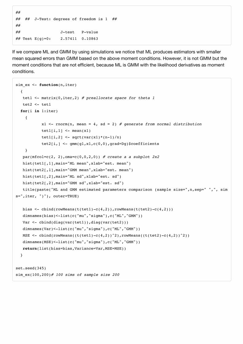
If we compare ML and GMM by using simulations we notice that ML produces estimators with smallermean squared errors than GMM based on the above moment conditions. However, it is not GMM but themoment conditions that are not efficient, because ML is GMM with the likelihood derivatives as momentconditions.

sim_ex <- function(n,iter)

{

tet1 <- matrix(0,iter,2) # preallocate space for theta 1

tet2 <- tet1

for(i in 1:iter)

{

x1 <- rnorm(n, mean = 4, sd = 2) # generate from normal distribution

tet1[i,1] <- mean(x1)

tet1[i,2] <- sqrt(var(x1)*(n-1)/n)

tet2[i,] <- gmm(g1,x1,c(0,0),grad=Dg)$coefficients

}

par(mfcol=c(2, 2),oma=c(0,0,2,0)) # create a a subplot 2x2

hist(tet1[,1],main="ML mean",xlab="est. mean")

hist(tet2[,1],main="GMM mean",xlab="est. mean")

hist(tet1[,2],main="ML sd",xlab="est. sd")

hist(tet2[,2],main="GMM sd",xlab="est. sd")

title(paste("ML and GMM estimated parameters comparison (sample size=",n,sep=" ",", sim

s=",iter, ")"), outer=TRUE)

bias <- cbind(rowMeans(t(tet1)-c(4,2)),rowMeans(t(tet2)-c(4,2)))

dimnames(bias)<-list(c("mu","sigma"),c("ML","GMM"))

Var <- cbind(diag(var(tet1)),diag(var(tet2)))

dimnames(Var)<-list(c("mu","sigma"),c("ML","GMM"))

MSE <- cbind(rowMeans((t(tet1)-c(4,2))2),rowMeans((t(tet2)-c(4,2))2))

dimnames(MSE)<-list(c("mu","sigma"),c("ML","GMM"))

return(list(bias=bias,Variance=Var,MSE=MSE))

}

set.seed(345)

sim_ex(100,200)# 100 sims of sample size 200

## $bias

## ML GMM

## mu -0.01406445 -0.01619955

## sigma -0.03723073 -0.07366727

##

## $Variance

## ML GMM

## mu 0.04530069 0.05574631

## sigma 0.02069728 0.02171330

##

## $MSE

## ML GMM

## mu 0.04527199 0.0557300

## sigma 0.02197992 0.0270316

If we increase the sample size (sample mean approaches the population mean) to 2,000, we notice that theGMM estimates improve, however the ML is still better.

set.seed(345)

sim_ex(100,2000) #100 sims of sample size 2000

## $bias

## ML GMM

## mu -7.842598e-05 -0.01057923

## sigma -1.590007e-02 -0.05185603

##

## $Variance

## ML GMM

## mu 0.04078809 0.04754989

## sigma 0.02060341 0.02293479

##

## $MSE

## ML GMM

## mu 0.04076770 0.04763803

## sigma 0.02084592 0.02561237

Nice treatment of GMM (with examples) can be found in Chapter 21 of book Modeling Financial TimeSeries with S-PLUS(r) (http://www.amazon.co.uk/dp/0387279652/ref=rdr_ext_tmb) . There are parts fromexamples above which follow this book.

http://www.amazon.co.uk/dp/0387279652/ref=rdr_ext_tmb

gmm

Documents