BIT 0006-3835/00/4004-0001 $15.002001, Vol. xx, No. x, pp. xxx–xxx c© Swets & Zeitlinger

GMRES, L-CURVES, AND DISCRETE ILL-POSEDPROBLEMS ∗

D. CALVETTI1, B. LEWIS2, and L. REICHEL3

Dedicated to Ake Bjorck on the occasion of his 65th birthday.

1Department of Mathematics, Case Western Reserve University, Cleveland, OH 44106.Email: dxc57@po.cwru.edu

2Department of Mathematics and Computer Science, Kent State University, Kent, OH44242. Email: blewis@mcs.kent.edu

3Department of Mathematics and Computer Science, Kent State University, Kent, OH44242. Email: reichel@mcs.kent.edu

Abstract.

The GMRES method is a popular iterative method for the solution of large linearsystems of equations with a nonsymmetric nonsingular matrix. This paper discussesapplication of the GMRES method to the solution of large linear systems of equationsthat arise from the discretization of linear ill-posed problems. These linear systemsare severely ill-conditioned and are referred to as discrete ill-posed problems. Weare concerned with the situation when the right-hand side vector is contaminated bymeasurement errors, and we discuss how a meaningful approximate solution of thediscrete ill-posed problem can be determined by early termination of the iterationswith the GMRES method. We propose a termination criterion based on the conditionnumber of the projected matrices defined by the GMRES method. Under certainconditions on the linear system, the termination index corresponds to the “vertex” ofan L-shaped curve.

AMS subject classification: 65F10, 65F22.

Key words: GMRES method, ill-posed problem, L-curve, regularization.

1 Introduction

The discretization of linear ill-posed problems gives rise to linear systems ofequations

Ax = b, A ∈ � n×n , x, b ∈ � n ,(1.1)

with a severely ill-conditioned matrix. Typically, the matrix has many “tiny”singular values, some of which may be vanishing. Following Hansen [12], we referto such linear systems as discrete ill-posed problems. We assume that the system(1.1) is consistent, and, in general, we would like to determine the solution of(1.1) of minimal norm.

∗Research supported in part by NSF grants DMS-9806702 and DMS-9806413.

2 D. CALVETTI, B. LEWIS, and L. REICHEL

Ill-posed problems arise, e.g., when seeking to determine the internal structureof a system by external measurements. The determination of the internal struc-ture of the sun by measurements from the earth is a classical ill-posed problem.Image restoration problems, in which one seeks to restore an image that hasbeen contaminated by blur and noise, provide other examples. In this appli-cation, often only a discretization of the contaminated image is available. Forinstance, the discretized image may be represented by an array of pixel values.The restoration of a contaminated discretized image is an example of a discreteill-posed problem. The matrix A then represents a blurring operator and oftenis the discretization of a compact integral operator with a smooth kernel. Weconsider an image restoration problem in Example 4.3 of Section 4.

In many linear discrete ill-posed problems that arise in the Sciences and En-gineering, the right-hand side vector is contaminated by measurement errorsd ∈ � n , which we also refer to as noise. Let b in (1.1) denote a noise-free, butunknown, vector, and let

bδ := b+ d(1.2)

be the available contaminated right-hand side vector. It is convenient to expressthe noise vector d as a multiple δ of a unit noise vector e, i.e.,

d = δe, ‖e‖ = 1.(1.3)

Here and throughout this paper ‖ · ‖ denotes the Euclidean vector norm or theassociated induced matrix norm. The norm δ of the error d is assumed to beunknown.

Since the vector b is not available, we cannot solve the linear system (1.1).Instead, we seek to determine an approximate solution of (1.1) by computing anapproximate solution of

Ax = bδ.(1.4)

In the image restoration problems discussed in Section 4, the vector bδ representsthe available discretized blurred and noisy image; the entries of the vector storepixel values. The vector b in (1.1) represents the discretized blurred but noise-free image and is not available. The computed approximate solution of (1.4)represents the discretized restored image.

The solution of (1.4), if it exists, generally is not a meaningful approximatesolution of (1.1) because of the severe ill-conditioning of the matrix A and thenoise d in the right-hand side vector bδ. Therefore, instead of solving the system(1.4), we replace it by a nearby linear system with a less ill-conditioned matrix,and solve the new linear system so obtained. This replacement is commonlyreferred to as regularization. We propose to implicitly define the nearby linearsystem by application of a few iterations of the GMRES method [15, 16], apopular iterative methods for the solution of large linear systems of equationswith a nonsingular nonsymmetric matrix.

The application of iterative methods to determine meaningful approximatesolutions to large discrete ill-posed problems has previously only been consideredfor problems with a symmetric matrix. For instance, the Conjugate Gradient(CG) method has been applied to solve the normal equations

ATAx = AT bδ(1.5)

associated with nonsymmetric linear systems (1.4); see Bjorck [1, 2], Hanke [8]and Hansen [12, Chapter 6] and references therein.

GMRES, L-CURVES, AND DISCRETE ILL-POSED PROBLEMS 3

It is important to terminate the iterations sufficiently early when applyingthe CG method to discrete ill-posed problems of the form (1.5). Hanke andHansen [10], and more recently Hansen [12, Chapter 6], describe how an L-curvecriterion can be used to determine when to terminate the iterations. Let xδj , j =0, 1, 2, · · · , denote the sequence of approximate solutions of (1.4) computed bythe CG method when applied to (1.5) with initial approximate solution xδ0 := 0,and introduce the associated sequence of residual vectors of the linear system(1.4),

rδj := bδ −Axδj , j = 0, 1, 2, · · · .(1.6)

Hansen [12, p. 142] points out that it follows from results by Hestenes and Stiefel[13] that

‖rδ0‖ ≥ ‖rδ1‖ ≥ ‖rδ2‖ ≥ · · · ,(1.7)

‖xδ0‖ ≤ ‖xδ1‖ ≤ ‖xδ2‖ ≤ · · · .(1.8)

Thus, the norm of the iterates xδj computed by the CG method increases and thenorm of the associated residual vectors (1.6) decreases as the iteration numberincreases.

Let φ(t) and ψ(t) be strictly increasing functions for t ≥ 0, and define thepoints qj := {φ(‖xδj‖), ψ(‖rδj‖)}, j = 0, 1, 2, · · · . Consider the graph obtainedby linear interpolation between adjacent points qj and qj+1 for j = 0, 1, 2, · · · .Because of the inequalities (1.7) and (1.8), the graph can be identified with apiecewise linear monotonically decreasing function. For many choices of increas-ing functions φ(t) and ψ(t), and for many discrete ill-posed problems, the graphlooks roughly like the letter “L.” Hanke and Hansen [10] therefore refer to thegraph as an L-curve and propose to choose the iterate xδk that corresponds tothe point qk at the “vertex” of the L-curve as the desired approximate solutionof (1.1). This choice can be motivated as follows. A vector xδj , that is associatedwith a residual error (1.6) of large norm, i.e., of norm much larger than δ, isa poor approximation of the solution to (1.4), and therefore, typically, also isa poor approximation of a solution to the noise-free linear system of equations(1.1). On the other hand, iterates xδj of large norm are likely to be contami-nated by propagated errors caused by the noise d in the right-hand side vectorbδ and by round-off errors introduced during the computation of xδj . Iterates xδjassociated with points qj near the “vertex” of the L-curve balance the errors inxδj caused by the inexact solution of the linear system (1.4) and the influence ofpropagated errors.

We remark that iterates xδj determined by the L-curve in the manner out-lined are not guaranteed to be suitable approximate solutions of (1.1). England Grever [6], Hanke [9], Hansen [12, Chapter 6] and Vogel [18] provide in-sightful discussions on properties and shortcomings of the L-curve applied tothe determination of regularized approximate solutions of ill-posed problems.To distinguish this L-curve from other L-curves discussed in the present paper,we will for clarity sometimes refer to it as the solution-norm L-curve for the CGmethod.

In most numerical examples of Section 4, we use the functions

φ(t) := log10(t), ψ(t) := log10(t), t > 0,(1.9)

4 D. CALVETTI, B. LEWIS, and L. REICHEL

and define the L-curve by linear interpolation between adjacent points qj andqj+1 for j = 1, 2, 3, · · · . The L-curve so obtained is independent of the pointq0 = {φ(‖xδ0‖), ψ(‖rδ0‖)}, which is not defined since xδ0 = 0.

For some discrete ill-posed problems (1.4), other choices of φ(t) and ψ(t) than(1.9) may give a more pronounced L-shape of the L-curve and therefore make iteasier to locate the “vertex.” This is illustrated in Section 4.

An analogue of the solution-norm L-curve described above can be defined whenthe iterates xδj are determined by the GMRES method applied to the solutionof linear discrete ill-posed problems (1.4). However, for many linear discreteill-posed problems, the curve so obtained does not look like the letter “L.” Thiscan be seen as follows. Let xδ0 := 0 be the initial approximate solution of (1.4)and introduce the Krylov subspaces

�j (A, bδ) = span{bδ, Abδ , . . . , Aj−1bδ}, j = 1, 2, 3, · · · .(1.10)

The GMRES method determines iterates xδj ∈�j (A, bδ), j = 1, 2, 3, · · · , that

satisfy‖bδ −Axδj‖ = min

x∈ � j (A,bδ)‖bδ −Ax‖.(1.11)

It follows from (1.11) and the relation�j−1 (A, bδ) ⊂ �

j (A, bδ) that the inequal-ities (1.7) hold for the residual vectors (1.6) associated with the GMRES iteratesxδj . However, the GMRES iterates are not guaranteed to satisfy the inequalities(1.8). Therefore, the graph obtained by linear interpolation between adjacentpoints qj and qj+1, for j = 0, 1, 2, · · · , where the points qj := {φ(‖xδj‖), ψ(‖rδj‖)}are determined by the GMRES iterates and the associated residual vectors, isnot L-shaped for many discrete ill-posed problems and it can be difficult to locatea “vertex” on the graph. This is illustrated by computed examples in Section 4.We refer to the graph as the solution-norm L-curve for the GMRES method.

This paper introduces a new L-curve, which is better suited for use with theGMRES method. It is obtained by replacing the abscissas φ(‖xδj‖) of the points

qj that define the solution-norm L-curve by φ(‖κδj‖), where κδj denotes the con-dition number of a projected matrix defined in the jth iteration of the GMRESmethod. The graph of the new L-curve describes a monotonically decreasingfunction, and we present sufficient conditions for it to have a “vertex.” Weuse the vertex to determine an approximate solution of the linear system (1.1);details and a motivation for this approach are presented in Section 2.

This paper is organized as follows. Section 2 discusses the GMRES method andintroduces the new L-curve, Section 3 presents conditions under which this curveexhibits a “vertex,” and computed examples are shown in Section 4. Concludingremarks can be found in Section 5.

2 The GMRES method and the condition L-curve

The GMRES method of Saad and Schultz [15, 16] is based on the Arnoldiprocess. We use the notation

< f, g >:= fT g, f, g ∈ � n ,

in the following description of the Arnoldi process.

Algorithm 2.1. The Arnoldi process

GMRES, L-CURVES, AND DISCRETE ILL-POSED PROBLEMS 5

Input: A ∈ � n×n , bδ ∈ � n , k ∈ � such that dim�k (A, bδ) = k;

Output: upper Hessenberg matrix Hδk = [hδi,j ]

ki,j=1 ∈

� k×k , orthonormal

basis {vδj}kj=1 of�k (A, bδ), f δk+1 ∈

� n ;

f δ1 := bδ;for j = 1, 2, . . . , k do

vδj := f δj /‖f δj ‖;f δj+1 := Avδj ;for i = 1, 2, . . . , j do

hδi,j :=< f δj+1, vδi >; f δj+1 := f δj+1 − hδi,jvδi ;

endfor i;if j < k

hδj+1,j := ‖f δj+1‖;endif;

endfor j;

The assumption that the number of iterations k in the algorithm is chosensmall enough so that dim

�k (A, bδ) = k holds simplifies the presentation of our

results, but is not essential. In fact, in the remainder of this section, we will fornotational simplicity assume that k is small enough, so that dim

�k+1 (A, bδ) =

k + 1. Then the vector f δk+1 determined by Algorithm 2.1 does not vanish.

Let V δj = [vδ1 , vδ2, . . . , v

δj ] for 1 ≤ j ≤ k. It follows from the construction of the

vector f δk+1 in Algorithm 2.1 that (V δk )T f δk+1 = 0. The relations for the matrix

entries hδj,k and vectors vδj and f δj+1 of the algorithm can be written in matrixform,

AV δk = V δkHδk + f δk+1e

Tk ,(2.1)

where ek denotes the kth axis vector. We refer to (2.1) as an Arnoldi decompo-sition of the matrix A.

Append the row ‖f δk+1‖eTk to the matrix Hδk and denote the (k+1)×k matrix

so obtained by Hδk . Define vδk+1 := f δk+1/‖f δk+1‖ and V δk+1 := [V δk , v

δk+1]. Then

(2.1) can be expressed asAV δk = V δk+1H

δk .(2.2)

The GMRES method solves the minimization problem (1.11) by expressingvectors x ∈ �

j as x = Vjy and using the decomposition (2.2) with k replaced byj. Thus,

‖Axδj − bδ‖ = minx∈ � j (A,bδ)

‖Ax− bδ‖ = miny∈� j

‖AV δj y − bδ‖

= miny∈ � j ‖V

δj+1(Hδ

j y − ‖bδ‖e1)‖ = miny∈ � j ‖H

δj y − ‖bδ‖e1‖(2.3)

= ‖Hδj yδj − ‖bδ‖e1‖,

where yδj solves the minimization problems (2.3). It follows that the jth iteratedetermined by the GMRES method can be expressed as

xδj = V δj yδj , yδj = (Hδ

j )†e1‖bδ‖ = (Hδj )†(V δj+1)T bδ,(2.4)

6 D. CALVETTI, B. LEWIS, and L. REICHEL

where (Hδj )† denotes the Moore-Penrose pseudo-inverse of the matrix Hδ

j . Hence,

xδj is the least-squares solution of minimal norm of the linear system of equations

Aδjx = bδ,(2.5)

whereAδj := V δj+1H

δj (V δj )T ∈ � n×n , j ≥ 1.(2.6)

Define the condition number of a matrix M by

κ(M) := ‖M‖‖M †‖.

Proposition 2.1. Assume that dim�k+1 (A, bδ) = k + 1. Then

‖Aδj‖ ≤ ‖Aδj+1‖,‖(Aδj)†‖ ≤ ‖(Aδj+1)†‖, j = 1, 2, . . . , k − 1,(2.7)

and it follows that the condition numbers κδj := κ(Aδj ) satisfy

κδj ≤ κδj+1, j = 1, 2, · · · , k − 1.(2.8)

Moreover,‖Aδj‖ ≤ ‖A‖, 1 ≤ j ≤ k,(2.9)

and if A is nonsingular, then

‖(Aδj)†‖ ≤ ‖A−1‖, 1 ≤ j ≤ k,(2.10)

andκδj ≤ κ(A), 1 ≤ j ≤ k.(2.11)

Proof. It follows from (2.6) and (Aδj )† = V δj (Hδ

j )†(V δj+1)T that

‖Aδj‖ = ‖Hδj ‖, ‖(Aδj )†‖ = ‖(Hδ

j )†‖.(2.12)

It therefore suffices to consider the matrices Hδj .

Let Hδj,0 ∈

� (j+2)×j denote the matrix obtained by appending a row with zero

entries to Hδj . The matrices Hδ

j,0 and Hδj have the same singular values, and

it follows that ‖Hδj,0‖ = ‖Hδ

j ‖ and ‖(Hδj,0)†‖ = ‖(Hδ

j )†‖. Appending the last

column of the matrix Hδj+1 to Hδ

j,0 yields Hδj+1. Therefore the singular values of

Hδj,0 interlace the singular values of Hδ

j+1; see, e.g., [7, p. 449]. The inequalities(2.7) follow from the interlacing property and (2.12).

The matrices Hδj and (Hδ

j )† are orthogonal projections of A and A†, respec-tively, and therefore the inequalities (2.9) and (2.10) hold. Finally, (2.8) followsfrom (2.7), and (2.11) from (2.9) and (2.10).

It is convenient to define κδ0 := 1. Then the inequality (2.8) also holds forj = 0.

We apply the GMRES method to the linear system (1.4) and determine theleast-squares solution of minimal norm xδj of a sequence of linear systems (2.5) for

GMRES, L-CURVES, AND DISCRETE ILL-POSED PROBLEMS 7

increasing values of j. Note that replacing the given linear system (1.4) by (2.5),and computing the minimal-norm least-squares solution of (2.5), constitutes aregularization method for the system (1.4), because we have replaced the ill-conditioned linear system (1.4) by the less ill-condition system (2.5), cf. (2.11).The inequalities (2.8) suggest that the condition numbers κδj of the matrices

Aδj of the regularized systems grow with j, and this behavior can generally be

observed in applications of the GMRES method. Moreover, the norm ‖A−Aδj‖decreases as j increases. It is important to terminate the GMRES iterationsafter a suitable number of iterations, say k of them, so that the matrix Aδk is nottoo ill-conditioned and Aδk is close to the matrix A. We refer to the iterationnumber as the regularization parameter.

Proposition 2.1 suggests a new L-curve for monitoring the progress of the itera-tions and for determining a suitable termination index k for the GMRES method.Let φ(t) and ψ(t) be strictly increasing functions for t ≥ 0, and define the pointsqj := {φ(κδj), ψ(‖rδj‖)} for j = 0, 1, 2, · · · . Consider the graph obtained by linearinterpolation between adjacent points qj and qj+1 for j = 0, 1, 2, · · · . Becauseof the inequalities (1.7) and (2.8), the graph can be identified with a piecewiselinear monotonically decreasing function. For many linear systems (1.4) thisgraph is shaped roughly like the letter “L.” We therefore refer to the graph asthe condition L-curve for the GMRES method. Let qk be the point at the “ver-tex” of the condition L-curve. We then choose xδk as an approximate solutionof (1.1). This choice seeks to balance the ill-conditioning of the matrices (2.6)in the linear systems (2.5) solved by the GMRES method, and the norm of theresidual errors (1.6) associated with the computed solutions.

The following result shows that the condition L-curve provides, up to thescaling factor ‖bδ‖/‖Hδ

1‖, an upper bound for the solution-norm L-curve for theGMRES method.

Theorem 2.2. Assume that dim�k+1 (A, bδ) = k + 1 and let xδj denote the

least-squares solution of minimal norm of the projected linear system (2.5) for1 ≤ j ≤ k. Then

‖xδj‖ ≤ κδj‖bδ‖‖Hδ

1‖, 1 ≤ j ≤ k.(2.13)

Proof. Formula (2.4) yields

‖xδj‖ = ‖yδj‖ ≤ ‖(Hδj )†‖‖bδ‖ = κδj

‖bδ‖‖Hδ

j ‖≤ κδj

‖bδ‖‖Hδ

1‖,

where the last inequality follows from (2.12) and (2.7).

3 The vertex of the condition L-curve

This section presents conditions on the linear system (1.1) and the noise d thatsecure that the condition L-curve for the GMRES method exhibits a “vertex.”The conditions imposed are chosen to make the analysis simple; they can easilybe weakened.

Let the matrix A have the spectral factorization

A = ZΛZ−1, Λ = diag[λ1, λ2, · · · , λn], Z = [z1, z2, . . . , zn],(3.1)

8 D. CALVETTI, B. LEWIS, and L. REICHEL

and assume that the eigenvalues λj are distinct and nonvanishing. Let the noise-free right-hand side vector b be a linear combination of m < n eigenvectors

b =m∑

j=1

αjzj(3.2)

with all coefficients αj 6= 0. Then the polynomial

pm(t) :=m∏

j=1

(1− t

λj)(3.3)

satisfiespm(A)b = 0.(3.4)

Assume that the noise d in (1.2) is such that

bδ =n∑

j=1

αδjzj(3.5)

with all coefficients αδj 6= 0.We will use the following notation. When δ = 0, we have d = 0, cf. (1.3),

and we omit the superscript δ. For instance, Algorithm 2.1 with input vector byields the orthonormal basis {vj}kj=1 of the Krylov subspace

�k (A, b) and the

upper Hessenberg matrix Hk.Proposition 3.1. Let xj , j = 1, 2, 3, · · · , denote the iterates determined by

the GMRES method when applied to the solution of the linear system (1.1) withthe noise-free right-hand side (3.2) and initial approximate solution x0 := 0.Then Axm = b and Axj 6= b for 0 ≤ j < m.

Let xδj , j = 1, 2, 3, · · · , denote the iterates determined by the GMRES methodwhen applied to the solution of the linear system (1.4) with the right-hand side(3.5) and initial approximate solution xδ0 := 0. Then Axn = bδ and Axj 6= bδ

for 0 ≤ j < n.Proof. The iterate xj determined by the GMRES method when applied to

the solution of the linear system (1.1) with initial approximate solution x0 := 0satisfies

‖b−Axj‖ = minx∈ � j (A,b)

‖b−Ax‖.(3.6)

Let � (0)j denote the set of all polynomials p of degree at most j such that p(0) = 1,

and assume that dim�j (A, b) = j. Then

minx∈ � j (A,b)

‖b−Ax‖ = minp∈ � (0)

j

‖p(A)b‖.(3.7)

It follows from the representation (3.2) that dim�j (A, b) = j for 1 ≤ j ≤ m.

Substituting (3.2) and the spectral factorization (3.1) into the right-hand sideof (3.7) shows that

minp∈� (0)

j

‖p(A)b‖ > 0, 1 ≤ j < m.(3.8)

GMRES, L-CURVES, AND DISCRETE ILL-POSED PROBLEMS 9

Let rj := b−Axj . Combining equations (3.6), (3.7) and (3.8) shows that rj 6= 0for 0 ≤ j < m. It follows that none of the iterates xj , 0 ≤ j < m, solve thelinear system of equations (1.1).

Since the polynomial pm defined by (3.3) is in the set � (0)m , we have

‖b−Axm‖ = minp∈� (0)

m

‖p(A)b‖ ≤ ‖pm(A)b‖ = 0,

where the last equality stems from (3.4). Thus, xm solves the linear system(1.1).

We turn to the solution of the linear system (1.4) with right-hand side (3.5).It follows from the representation (3.5) that dim

�j (A, bδ) = j for 1 ≤ j ≤ n.

Substituting the spectral factorization (3.1) into the minimization problem (1.11)shows that the iterates xδj satisfy Axδj 6= bδ for 1 ≤ j < n, and that Axδn = bδ.

The following definitions help us to discuss the graph of the condition L-curve.Let qj = {sj , tj}, j = 0, 1, 2, · · · , denote points in

� 2 . We say that q0 is larger(smaller) than q1, and write q0 ≥ q1 (q0 ≤ q1) if s0 = s1 and t0 ≥ t1 (t0 ≤ t1).The point q0 is said to lie below the line segment � ⊂ � 2 if there is a pointq1 ∈ � , such that q0 ≤ q1. We say that a set of points � = {qj}`j=0 is ordered

if s0 ≤ s1 ≤ · · · ≤ s`. An ordered triple of points {qj}2j=0 is said to determine avertex if the point q1 lies below the line segment that joins the points q0 and q2.We say that an ordered point set � = {qj}`j=0 has a vertex if the set contains

an ordered triple {qi}j+1i=j−1 that determines a vertex.

Proposition 3.2. Let � = {qj}`j=0 be an ordered set of points in� 2 and

assume that one of the points, say qk, lies below the line segment that joins q0

and q`. Then the set � has a vertex.Proof. The statement follows immediately from the definitions.We are now in a position to discuss the existence of a vertex of the condition

L-curve. Let φ(t) and ψ(t) be strictly increasing functions for t ≥ 0, and let theset of points

� = {qj}nj=0, qj := {φ(κδj), ψ(‖rδj‖)},(3.9)

where the condition numbers κδj are defined in Proposition 2.1, be determinedby the GMRES method applied to the solution of the linear system of equations(1.4) with right-hand side vector (3.5) and initial approximate solution xδ0 := 0.

It follows from the inequalities (2.8) that the set (3.9) is ordered. The graphobtained by linear interpolation between adjacent points qj and qj+1 for j =0, 1, 2, · · · , is the condition L-curve for the GMRES method. We say that thecondition L-curve has a vertex if the set of points (3.9) has a vertex.

Theorem 3.3. Let the right-hand side vector b in (1.1) be of the form (3.2),and assume that the unit noise vector e in (1.3) is such that the right-hand sidevector bδ given by (1.2) can be expressed as (3.5) with all coefficients αδj 6= 0 for

all δ > 0 sufficiently small.1

Apply the GMRES method to the solution of the linear system of equations(1.4) with a right-hand side vector bδ with the stated properties, and with initialapproximate solution xδ0 := 0. Let the point set (3.9) be determined by the GM-RES method. Then the condition L-curve for the GMRES method determinedby this point set has a vertex for any δ > 0 sufficiently small.

1We vary δ, but keep e fixed

10 D. CALVETTI, B. LEWIS, and L. REICHEL

The proof of the theorem is a consequence of the following result.Lemma 3.4. Let the GMRES method applied to the linear system (1.4) with

right-hand side vector bδ given by (3.5) and initial approximate solution xδ0 := 0give the iterates xδj , j = 1, 2, 3, · · · , and associated residual vectors rδj definedby (1.6). Then

‖rδm‖ ≤m∏

j=1

(1 +‖A‖|λj |

)δ.(3.10)

Proof. The least-squares problem (1.11) with j replaced by m can be writtenas

‖rδm‖ = minp∈� (0)

m

‖p(A)bδ‖,

cf. (3.7). Since the polynomial pm defined by (3.3) is in � (0)m , it follows that

‖rδm‖ ≤ ‖pm(A)bδ‖ ≤ ‖pm(A)b‖+ ‖pm(A)(bδ − b)‖ ≤ ‖pm(A)‖δ,(3.11)

where the last inequality follows from (3.4) and ‖bδ − b‖ = δ. Moreover,

‖pm(A)‖ ≤m∏

j=1

‖I − 1

λjA‖ ≤

m∏

j=1

(1 +‖A‖|λj |

).(3.12)

Combining equations (3.11) and (3.12) completes the proof.Proof of Theorem 3.3. Assume that δ > 0 satisfies ‖b‖ > δ. Note that

q0 = {φ(0), ψ(‖bδ‖)} ≥ {φ(0), ψ(‖b‖ − δ)} and qn = {φ(κ(A)), ψ(0)}. We willshow that for any δ > 0 sufficiently small, the point qm = {φ(κδm), ψ(‖rδm‖)} liesbelow the line segment between the points q0 and qn.

By Lemma 3.4, there is a constant cm, independent of δ > 0, such that

ψ(‖rδm‖) ≤ ψ(cmδ).(3.13)

Application of the GMRES method to the solution of the linear system ofequations (1.1) with right-hand side vector (3.2) and initial approximate solutionx0 := 0 yields a sequence of upper Hessenberg-like matrices Hj ∈

� (j+1)×j

and iterates xj , j = 1, 2, · · · ,m. By Proposition 3.1, we have Axm−1 6= b andAxm = b. Therefore, the last row of Hm vanishes and the columns of Hm arelinearly independent; see Saad [15, Propositions 6.10 and 6.11].

The matrix Hδm, obtained by application of Algorithm 2.1 with k = m to the

matrix A and initial vector (3.5), depends continuously on δ, for δ > 0 suf-ficiently small and e fixed. Since the columns of the matrix Hδ

m are linearlyindependent for all δ > 0 sufficiently small, the pseudo-inverse (Hm)† also de-pends continuously on δ for all δ > 0 sufficiently small. Thus,

limδ↘0‖Hδ

m‖ = ‖Hm‖, limδ↘0‖(Hδ

m)†‖ = ‖(Hm)†‖.(3.14)

Let the condition numbers κδj be defined as in Proposition 2.1. We obtain from(2.12) and (3.14) that

limδ↘0

κδm = κm := ‖Hm‖‖(Hm)†‖,

GMRES, L-CURVES, AND DISCRETE ILL-POSED PROBLEMS 11

We conclude from (3.13) and (3.14) that the point qm can be positioned arbi-trarily close to q∗ := {φ(κm), ψ(0)} by choosing δ > 0 sufficiently small. Theobservation that the ordered triple {q0, q

∗, qn} forms a vertex concludes theproof. �

4 Computed Examples

The computations for the first two examples were carried out on an Intel Pen-tium workstation with Matlab 5.3. The third example presents an applicationto image restoration and requires significantly more computational work andcomputer storage than the first examples. The computations for the latter ex-ample were carried out on a networked cluster of Intel Pentium workstationsusing Octave 2.0.16. The unit round-off for all examples was 2 · 10−16.

The examples compare the condition and solution-norm L-curves for the GM-RES method, the solution-norm L-curve for the CG method applied to the nor-mal equations (1.5) and the solution-norm L-curve for Truncated Singular ValueDecomposition (TSVD). The latter method is often used for the solution of smalllinear discrete ill-posed problems. We outline the method; details are discussed,e.g., by Hansen [12, Chapters 3 and 5]. Introduce the singular value decompo-sition

A = USW T ,

where

U = [u1, u2, . . . , un] ∈ � n×n , UTU = I,W = [w1, w2, . . . , wn] ∈ � n×n , W TW = I,

S = diag[σ1, σ2, . . . , σn] ∈ � n×n , σ1 ≥ σ2 ≥ · · · ≥ σn ≥ 0,

and I denotes the identity matrix. Define the diagonal matrices

Sk = diag[σ1, σ2, . . . , σk, 0, . . . , 0] ∈ � n×n .

The TSVD method gives the approximate solutions

xδk := WS†kUT bδ, 0 ≤ k ≤ n,(4.1)

of (1.4), where we define xδ0 := 0. The representations

xδk =k∑

j=1

uTj bδ

σjwj , 1 ≤ k ≤ n,

show that ‖xδk‖ grows with k. It is easy to establish that the norm of theassociated residual vectors rδk = bδ −Axδk decreases as k increases.

Let φ(t) and ψ(t) be strictly increasing functions for t ≥ 0 and define thepoints qk := {φ(‖xδk‖), ψ(‖rδk‖)}, 0 ≤ k ≤ n, where xδk is given by (4.1) and rδkis the associated residual vector (1.6). We refer to the graph obtained by linearinterpolation between adjacent points qk and qk+1 as the solution-norm L-curvefor the TSVD method. In all graphs of L-curves in this section, except for thosein Figures 4.6 and 4.7, we used the φ(t) and ψ(t) given by (1.9).

Example 4.1. We compare the condition L-curve for the GMRES method withthe solution-norm L-curves for the GMRES and TSVD methods. This example

12 D. CALVETTI, B. LEWIS, and L. REICHEL

0 1 2 3 4 5 6 7 8 9−12

−10

−8

−6

−4

−2

0

2

log10

(κjδ)

Figure 4.1: Example 4.1: Condition L-curve for the GMRES method (solidcurve) with points qj = {log10 κ

δj , log10 ‖rδj‖}, j = 1, 2, 3, marked by “o.” The

points qj := {log10 κδj , log10(‖xδj − x‖/‖x‖)}, j = 1, 2, 3, marked by “×,” display

the relative error of the iterates xδj . Points qj with adjacent indices are connectedby dotted line segments.

illustrates that the GMRES method when combined with the condition L-curvecan give a more accurate approximation of the exact solution of (1.1) than theGMRES and TSVD methods when used in conjunction with the solution-normL-curves.

Define the 3×3 matrix A in the linear system (1.1) by its spectral factorization(3.1), where

Z = [z1, z2, z3] =

1 1.0001 1−1 −1.0001 0

0 0.0001 0

, Λ = diag[1, 2, 3].(4.2)

Letx := z2 + z3(4.3)

and define the noise-free right-hand side vector in (1.1) by b := Ax. The linearsystem (1.1) so obtained is consistent and has an ill-conditioned matrix, withκ(A) = 1.0×108. Introduce the noise vector d = [0, 6×10−4, 4×10−4]T of normδ = 7.2× 10−4, and define the noisy right-hand side bδ by (1.2).

The discussion of Section 3 shows that the linear system (1.1) with the noise-free right-hand side vector b can be solved in two iterations by the GMRESmethod when the initial vector is chosen to be x0 = 0. The solution of the linear

GMRES, L-CURVES, AND DISCRETE ILL-POSED PROBLEMS 13

0 0.05 0.1 0.15 0.2 0.25 0.3 0.35−12

−10

−8

−6

−4

−2

0

2

log10

(||xjδ||)

Figure 4.2: Example 4.1: Solution-norm L-curve for the GMRES method (solidcurve) with points qj = {log10 ‖xδj‖, log10 ‖rδj‖}, j = 1, 2, 3, marked by “o.”

The points qj := {log10 ‖xδj‖, log10(‖xδj − x‖/‖x‖)}, j = 1, 2, 3, marked by “×,”

display the relative error of the iterates xδj . Points qj with adjacent indices areconnected by dotted line segments.

system (1.4) with the right-hand side vector bδ requires three iterations with thesame initial vector.

Figure 4.1 displays the condition L-curve for the GMRES method (solid linesegments). The points qj := {log10 κ

δj , log10 ‖rδj‖}, j = 1, 2, 3, that define the

L-curve are marked by “o.” If the computations were carried out in exact arith-metic, then rδ3 would vanish. In order to easily be able to compare the conditionL-curve with the solution-norm L-curve, we do not display the point q0. Notethat the L-curve has a vertex at q2.

Figure 4.1 also shows the logarithm of the relative error log10(‖xδj − x‖/‖x‖),where xδj denotes the iterates determined by the GMRES method and x is theexact solution (4.3) of the linear system (1.1). The figure displays the pointsqj := {log10 κ

δj , log10(‖xδj − x‖/‖x‖)}, j = 1, 2, 3, marked by “x.” Consecutive

points qj are connected by dotted line segments. The figure shows that thesmallest relative error is achieved by the iterate xδ2, which corresponds to thevertex of the condition L-curve.

Figure 4.2 shows the solution-norm L-curve for the GMRES method definedby the points qj := {log10 ‖xδj‖, log10 ‖rδj‖}, j = 1, 2, 3. These points are marked

by “o.” We omit the point q0 because the logarithm is not defined for xδ0 = 0.Since the points qj , j = 1, 2, 3, are not ordered, the solution-norm L-curve does

14 D. CALVETTI, B. LEWIS, and L. REICHEL

−3.5 −3 −2.5 −2 −1.5 −1 −0.5 0 0.5−12

−10

−8

−6

−4

−2

0

2

log10

(||xjδ||)

Figure 4.3: Example 4.1: Solution norm L-curve for the TSVD method (solidcurve) with points qj = {log10 ‖xδj‖, log10 ‖rδj‖}, j = 1, 2, 3, marked by “o.”

The points qj := {log10 ‖xδj‖, log10(‖xδj − x‖/‖x‖)}, j = 1, 2, 3, marked by “×,”

display the relative error of the approximate solutions xδj . Points qj with adjacentindices are connected by dotted line segments.

not display a vertex. The figure also shows the logarithm of the relative errorsin the computed iterates, similarly as Figure 4.1. It is not obvious from thesolution-norm L-curve that xδ2 is the best approximate solution of (1.4).

Figure 4.3 presents the solution-norm L-curve for the TSVD method. Thepoints qj := {log10 ‖xδj‖, log10 ‖rδj‖}, j = 1, 2, 3, that determine the L-curve areordered, but the curve does not display a vertex. Thus, the solution-norm L-curve for the TSVD method does not clearly indicate which xδj should be chosenas an approximate solution of (1.4). The figure also displays the logarithm of therelative errors in the computed approximate solutions xδj . Note that the norm oferrors in the approximate solutions determined by the TSVD method is at leastas large, and for j = 2 much larger, than the norm of the error in the iteratescomputed by the GMRES method. �

Example 4.2. The inversion of the Laplace transform∫ ∞

0

exp(−st)x(t)dt = b(s), s ≥ 0,(4.4)

where b is a given function and x is to be determined, is a classical ill-posedproblem. Let

b(s) :=1

s− 2

2s+ 1.

GMRES, L-CURVES, AND DISCRETE ILL-POSED PROBLEMS 15

0 1 2 3 4 5 6 7 8 9 10−3

−2

−1

0

1

2

3

4

5

log10

(κjδ)

Figure 4.4: Example 4.2: Condition L-curve for the GMRES method (solidcurve) with points qj = {log10 κ

δj , log10 ‖rδj‖}, 1 ≤ j ≤ 14, marked by “o.” The

points qj := {log10 κδj , log10(‖xδj−x‖/‖x‖)}, 1 ≤ j ≤ 14, marked by “×,” display

the relative error of the iterates xδj . Points qj with adjacent indices are connectedby dotted line segments.

Then the solution of (4.4) is given by

x(t) := 1− exp(−t/2).(4.5)

We discretize the integral equation (4.4) by software written in Matlab by Hansen[11]. The integral is replaced by a 100-point Gauss-Laguerre quadrature ruleand the equation so obtained is required to be satisfied at the collocation pointssj := j/10, 1 ≤ j ≤ 100. This determines the matrix A ∈ � 100×100 and the

entries bj := b(sj) of the right-hand side vector b ∈ � 100 of the linear system(1.1). Let the noise vector d ∈ � 100 have normally distributed random entrieswith zero mean and with variance chosen so that δ = 1 · 10−4; cf. (1.3). Weobtain the noisy right-hand side vector from (1.2). This defines the linear systemof equations (1.4).

Let xδj denote the iterates computed by the GMRES method when applied

to the solution of (1.4) with initial approximate solution xδ0 := 0. Figure 4.4is analogous to Figure 4.1 and shows the condition L-curve for the GMRESmethod as well as the logarithm of the relative error of the iterates. We considerthe tabulation of the function (4.5) at the 100 nodes of the Gauss-Laguerrequadrature rule as the “exact solution” x when computing the relative error‖xδj − x‖/‖x‖.

Figure 4.4 shows the condition L-curve to have two vertices, each of which is

16 D. CALVETTI, B. LEWIS, and L. REICHEL

0.5 1 1.5 2 2.5 3 3.5 4−3

−2

−1

0

1

2

3

log10

(||xjδ||)

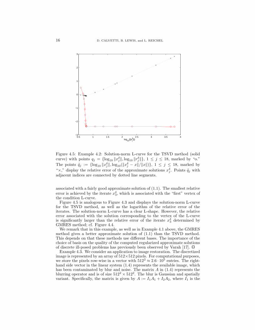
Figure 4.5: Example 4.2: Solution-norm L-curve for the TSVD method (solidcurve) with points qj = {log10 ‖xδj‖, log10 ‖rδj‖}, 1 ≤ j ≤ 18, marked by “o.”

The points qj := {log10 ‖xδj‖, log10(‖xδj − x‖/‖x‖)}, 1 ≤ j ≤ 18, marked by

“×,” display the relative error of the approximate solutions xδj . Points qj withadjacent indices are connected by dotted line segments.

associated with a fairly good approximate solution of (1.1). The smallest relativeerror is achieved by the iterate xδ3, which is associated with the “first” vertex ofthe condition L-curve.

Figure 4.5 is analogous to Figure 4.3 and displays the solution-norm L-curvefor the TSVD method, as well as the logarithm of the relative error of theiterates. The solution-norm L-curve has a clear L-shape. However, the relativeerror associated with the solution corresponding to the vertex of the L-curveis significantly larger than the relative error of the iterate xδ3 determined byGMRES method; cf. Figure 4.4.

We remark that in this example, as well as in Example 4.1 above, the GMRESmethod gives a better approximate solution of (1.1) than the TSVD method.This depends on that these methods use different bases. The importance of thechoice of basis on the quality of the computed regularized approximate solutionsof discrete ill-posed problems has previously been observed by Varah [17]. �

Example 4.3. We consider an application to image restoration. The discretizedimage is represented by an array of 512×512 pixels. For computational purposes,we store the pixels row-wise in a vector with 5122 ≈ 2.6 · 105 entries. The right-hand side vector in the linear system (1.4) represents the available image, whichhas been contaminated by blur and noise. The matrix A in (1.4) represents theblurring operator and is of size 5122 × 5122. The blur is Gaussian and spatiallyvariant. Specifically, the matrix is given by A := I1A1 + I2A2, where I1 is the

GMRES, L-CURVES, AND DISCRETE ILL-POSED PROBLEMS 17

0 10 20 30 40 50 60 70 80 90 1002.4

2.6

2.8

3

3.2

3.4

3.6

3.8

κjδ

Figure 4.6: Example 4.3: Condition L-curve for the GMRES method.

diagonal matrix, whose first 5122/2 diagonal entries are one, and the remainingentries zero, and I2 := I − I1. The matrices Ai are Kronecker products ofbanded Toeplitz matrices Ti, which represent Gaussian blur in one dimension.

Thus, Ai := Ti ⊗ Ti, where the matrices Ti = [t(i)j,k]512

j,k=1, i = 1, 2, are given by

t(i)j,k :=

{1

ρi√

2πexp(− (j−k)2

2ρ2i

), if |j − k| ≤ 12ρi,

0, otherwise.

In the computations, we let ρ1 := 4 and ρ2 := 4.5. This gave matrices Ti withcondition numbers greater that 1 · 1018, i.e., the matrices Ti were numericallysingular. The blurring matrix A so obtained is nonsymmetric. It representsdifferent blur in the upper and lower halves of the image.

Given the discretization of an “original” noise-free and blur-free image x ∈� 5122

, we generated a blurred and noisy image bδ := Ax + d, where d is anoise vector with normally distributed random entries with zero mean and withvariance chosen so that ‖d‖/‖b‖ = 5.0 × 10−3. The original image x in thisexample is “Antarctic Penguins” from NASA, image number AC86-0614-22.

Figure 4.6 displays the condition L-curve for the GMRES method when appliedto the solution of (1.4) with initial approximate solution xδ0 := 0. Let xδj denote

the iterates generated by the GMRES method and let rδj be the associated

residual vectors (1.6). The condition numbers κδj are defined in Proposition 2.1.The condition L-curve shown is determined by the point set

� = {qj}10j=1, qj := {φ(κδj ), ψ(‖rδj‖)}

18 D. CALVETTI, B. LEWIS, and L. REICHEL

6.18 6.2 6.22 6.24 6.26 6.28 6.3 6.32

x 104

2.4

2.6

2.8

3

3.2

3.4

3.6

3.8

||xjδ||

Figure 4.7: Example 4.3: Solution-norm L-curve for the CG method applied tothe normal equations (1.5).

withφ(t) := t, ψ(t) := log10 t.(4.6)

This choice of φ(t) and ψ(t) gives a more pronounced L-shape than the choice(1.9).

The L-curve suggests that xδ4 may be a good approximation of the originalnoise-free and blur-free image. This is verified by Figure 4.8, which shows thegiven blurred and noisy image in the upper-left corner, and then row-wise, fromtop to bottom, displays the images determined by the GMRES method after2, 4, 6, 8 and 10 iterations. The amplified noise in the images obtained whencarrying out 8 and 10 iterations is clearly visible.

For comparison, we also determined approximate solutions of the linear system(1.1) by applying the CG method to the normal equations (1.5). We used theimplementation CGLS described by Bjorck [2, Chapter 7]. Related methods havebeen applied to the restoration of astronomical images with spatially-variantblur; see Nagy and O’Leary [14] for a discussion.

Figure 4.7 shows the solution-norm L-curve for the CG method applied to thenormal equations (1.5) with initial approximate solution xδ0 := 0. Denote theiterates determined by the CG method by xδj and let rδj denote the associatedresidual vector (1.6). The solution-norm L-curve shown is determined by thepoint set

� = {qj}25j=1, qj := {φ(‖xδj‖), ψ(‖rδj‖)}

with φ(t) and ψ(t) given by (4.6). This choice of φ(t) and ψ(t) makes it easy tocompare the graph with the condition L-curve of Figure 4.6. The solution-norm

GMRES, L-CURVES, AND DISCRETE ILL-POSED PROBLEMS 19

L-curve has a fairly pronounced vertex at the point q19 and this suggests thatthe iterate xδ19 may be a good approximation of the original image noise-free andblur-free image.

Figure 4.9 shows the given blurred and noisy image in the upper-left cor-ner (same image as in the upper-left corner of Figure 4.8), and then row-wise,from top to bottom, displays the images determined by the CG method after5, 10, 15, 19 and 25 iterations. Each iteration requires the evaluation two matrix-vector products, one with the matrix A and one with its transpose. Much blurhas been removed in the image obtained after 19 iterations, however, the figuredisplays “ringing.” In the present example, the images restored by the GMRESmethod do not suffer from “ringing.” Experience from the restoration of nu-merous images by the GMRES and CGLS methods suggests that the GMRESmethod typically gives a better restoration with less computational work. �

5 Conclusion and related work

The GMRES method can be applied to compute meaningful approximate so-lutions of linear discrete ill-posed problems with a right-hand side vector that iscontaminated by errors. The termination criterion for the iterations is impor-tant. The condition L-curve is well suited for this purpose for many problems.Comparison with the conjugate gradient method applied to the normal equationssuggests that for many problems the GMRES method may be able to computea meaningful approximate solution with less work.

We remark that superior performance of the GMRES also can be observedwhen the iterations are terminated by the discrepancy principle; see [3] for nu-merical examples.

The condition L-curve introduced in the present paper for use with the GM-RES method can be used together with many regularization methods. For in-stance, its use with the MINRES and MR-II iterative methods is described in[4].

This paper focuses on some computational issues related to the application ofthe GMRES method to the solution of discrete ill-posed problems. The investi-gation [5] sheds light on the regularizing property of the GMRES method.

REFERENCES

1. A. Bjorck, A bidiagonalization algorithm for solving large and sparse ill-posed sys-tems of linear equations, BIT, 28 (1988), pp. 659–670.

2. A. Bjorck, Numerical Methods for Least Squares Problems, SIAM, Philadelphia,1996.

3. D. Calvetti, B. Lewis and L. Reichel, Restoration of images with spatially variantblur by the GMRES method, in Advanced Signal Processing Algorithms, Architec-tures, and Implementations X, ed. F. T. Luk, Proceedings of the Society of Photo-Optical Instrumentation Engineers (SPIE), vol. 4116, The International Society forOptical Engineering, Bellingham, WA, 2000, pp. 364–374.

4. D. Calvetti, B. Lewis and L. Reichel, An L-curve for the MINRES method, inAdvanced Signal Processing Algorithms, Architectures, and Implementations X, ed.F. T. Luk, Proceedings of the Society of Photo-Optical Instrumentation Engineers(SPIE), vol. 4116, The International Society for Optical Engineering, Bellingham,WA, 2000, pp. 385–395.

20 D. CALVETTI, B. LEWIS, and L. REICHEL

5. D. Calvetti, B. Lewis and L. Reichel, On the regularizing properties of the GMRESmethod, Numer. Math., to appear.

6. H. W. Engl and W. Grever, Using the L-curve for determining optimal regulariza-tion parameters, Numer. Math., 69 (1994), pp. 25–31.

7. G. H. Golub and C. F. Van Loan, Matrix Computations, 3rd ed., Johns HopkinsUniversity Press, Baltimore, 1996.

8. M. Hanke, Conjugate Gradient Type Methods for Ill-Posed Problems, Longman,Harlow, 1995.

9. M. Hanke, Limitations of the L-curve method in ill-posed problems, BIT, 36 (1996),pp. 287–301.

10. M. Hanke and P. C. Hansen, Regularization methods for large-scale problems, Surv.Math. Ind., 3 (1993), pp. 253–315.

11. P. C. Hansen, Regularization Tools: A Matlab package for analysis and solution ofdiscrete ill-posed problems, Numer. Algorithms, 6 (1994), pp. 1–35.

12. P. C. Hansen, Rank-Deficient and Discrete Ill-Posed Problems, SIAM, Philadelphia,1998.

13. M. R. Hestenes and E. Stiefel, Methods of conjugate gradients for solving linearsystems, J. Res. Nat. Bur. Standards, 49 (1952), pp. 409–436.

14. J. G. Nagy and D. P. O’Leary, Restoring images degraded by spatially-variant blur,SIAM J. Sci. Comput., 19 (1998), pp. 1063–1082.

15. Y. Saad, Iterative Methods for Sparse Linear Systems, PWS, Boston, 1996.

16. Y. Saad and M. H. Schultz, GMRES: a generalized minimal residual method forsolving nonsymmetric linear systems, SIAM J. Sci. Stat. Comput., 7 (1986), pp.856–869.

17. J. M. Varah, Pitfalls in the numerical solution of linear ill-posed problems, SIAMJ. Sci. Stat. Comput., 4 (1983), pp. 164–176.

18. C. R. Vogel, Non-convergence of the L-curve regularization parameter selectionmethod, Inverse Problems, 12 (1996), pp. 535–547.

GMRES, L-CURVES, AND DISCRETE ILL-POSED PROBLEMS 21

Figure 4.8: Example 4.3: Image restoration by the GMRES method. Row-wisefrom top-left to bottom-right: the given image that is contaminated by blurand noise, the restored images after 2, 4, 6, 8, and 10 iterations by the GM-RES method. The condition L-curve for the GMRES method suggests that 4iterations should be carried out.

22 D. CALVETTI, B. LEWIS, and L. REICHEL

Figure 4.9: Example 4.4: Image restoration by the CG method applied to thenormal equations (1.5). Row-wise from top-left to bottom-right: the given imagethat is contaminated by blur and noise, the restored images after 5, 10, 15, 19,and 25 iterations by the CG method. The solution-norm L-curve for the CGmethod suggests that 19 iterations should be carried out.