gms: grid-based motion statistics for fast, ultra-robust ...gms is robust to various challenging...

International Journal of Computer Vision (2020) 128:1580–1593https://doi.org/10.1007/s11263-019-01280-3

GMS: Grid-Based Motion Statistics for Fast, Ultra-robust FeatureCorrespondence

Jia-Wang Bian1,2 ·Wen-Yan Lin3 · Yun Liu4 · Le Zhang5 · Sai-Kit Yeung6 ·Ming-Ming Cheng4 · Ian Reid1,2

Received: 8 August 2018 / Accepted: 10 December 2019 / Published online: 17 December 2019© The Author(s) 2019

AbstractFeature matching aims at generating correspondences across images, which is widely used in many computer vision tasks.Although considerable progress has been made on feature descriptors and fast matching for initial correspondence hypothe-ses, selecting good ones from them is still challenging and critical to the overall performance. More importantly, existingmethods often take a long computational time, limiting their use in real-time applications. This paper attempts to separate truecorrespondences from false ones at high speed. We term the proposed method (GMS) grid-based motion Statistics, whichincorporates the smoothness constraint into a statistic framework for separation and uses a grid-based implementation forfast calculation. GMS is robust to various challenging image changes, involving in viewpoint, scale, and rotation. It is alsofast, e.g., take only 1 or 2 ms in a single CPU thread, even when 50K correspondences are processed. This has importantimplications for real-time applications. What’s more, we show that incorporating GMS into the classic feature matching andepipolar geometry estimation pipeline can significantly boost the overall performance. Finally, we integrate GMS into thewell-known ORB-SLAM system for monocular initialization, resulting in a significant improvement.

Keywords Feature matching · Epipolar geometry · Visual SLAM · Structure-from-motion · GMS

1 Introduction

Feature matching is one of the most fundamental problemsin the computer vision community. It aims to generate cor-respondences across different views of an object or scene,which is widely used in many vision tasks such as structure-from-motion (Schonberger and Frahm 2016) and VisualSLAM (Davison et al. 2007; Mur-Artal et al. 2015). Typi-cal solutions rely on feature detectors (Harris and stephens1988), descriptors (Lowe 2004), and matchers (Muja and

Communicated by Jiri Matas.

B Jia-Wang [email protected]

1 The University of Adelaide, Adelaide, Australia

2 Australian Centre for Robotic Vision, Brisbane, Australia

3 Singapore Management University, Singapore, Singapore

4 Nankai University, Tianjin, China

5 Agency for Science, Technology and Research, Singapore,Singapore

6 Hong Kong University of Science and Technology, HongKong, China

Lowe 2009) for generating putative correspondences. Thenthe selected correspondences are taken as input in a high-leveltask, where a RANSAC (Fischler and Bolles 1981) basedestimator is often applied to fit a geometricmodel and removeoutliers simultaneously. Although considerable progress hasbeen made on features, matchers, and estimators, the overallperformance is still limited by the false correspondences, i.e,they cause robust estimators to fail to find a correctmodel andtrue inliers. This problem is critical but received relativelyless attention than other problems motioned above. Moreimportantly, existing approaches are time-consuming (Linet al. 2017), limiting their use in real-time applications. Toaddress this gap, we propose a novel method termed (GMS)grid-based motion statistics for separating true correspon-dences from false ones at high speed.

The proposed method relies on the motion smoothnessconstraint, i.e, we assume that neighboring pixels in oneimage would move together since they often land in one rigidobject or structure. Although the assumption is not generallycorrect, e.g., violated in image boundaries, it suits to mostregular pixels. This is sufficient for our purpose since we arenot targeting a final correspondence solution but a set of high-quality correspondences for RANSAC-like approaches. The

123

http://crossmark.crossref.org/dialog/?doi=10.1007/s11263-019-01280-3&domain=pdf

http://orcid.org/0000-0003-2046-3363

International Journal of Computer Vision (2020) 128:1580–1593 1581

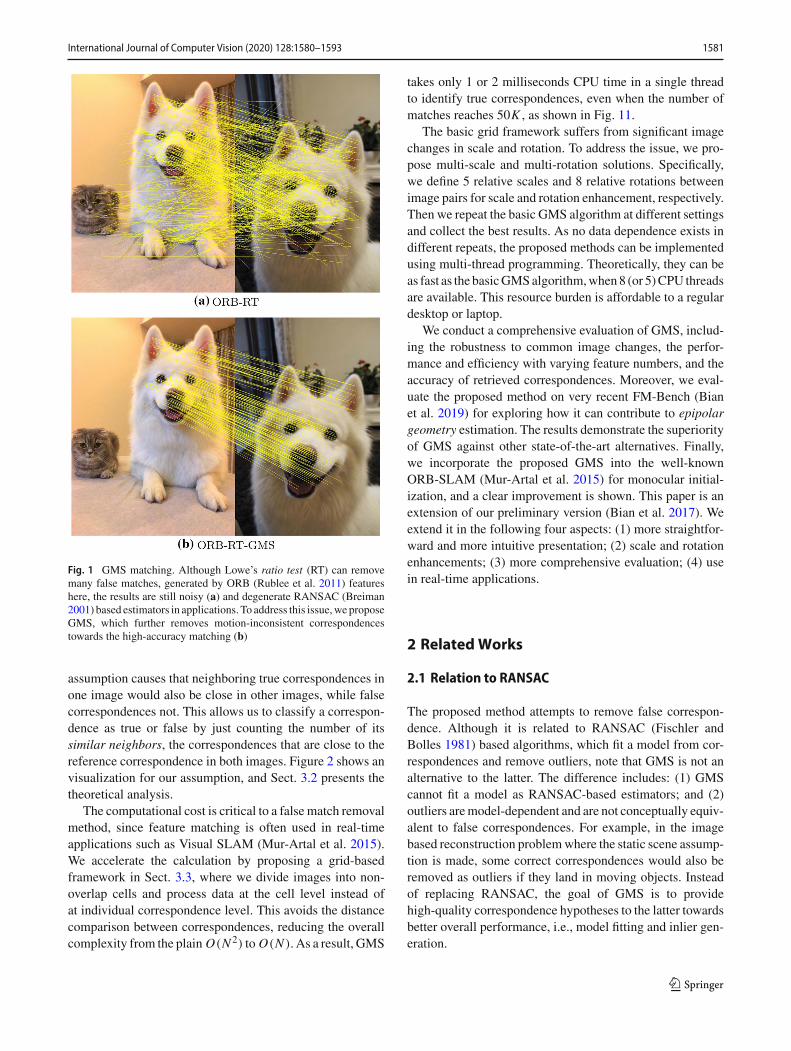
Fig. 1 GMS matching. Although Lowe’s ratio test (RT) can removemany false matches, generated by ORB (Rublee et al. 2011) featureshere, the results are still noisy (a) and degenerate RANSAC (Breiman2001) based estimators in applications. To address this issue,weproposeGMS, which further removes motion-inconsistent correspondencestowards the high-accuracy matching (b)

assumption causes that neighboring true correspondences inone image would also be close in other images, while falsecorrespondences not. This allows us to classify a correspon-dence as true or false by just counting the number of itssimilar neighbors, the correspondences that are close to thereference correspondence in both images. Figure 2 shows anvisualization for our assumption, and Sect. 3.2 presents thetheoretical analysis.

The computational cost is critical to a false match removalmethod, since feature matching is often used in real-timeapplications such as Visual SLAM (Mur-Artal et al. 2015).We accelerate the calculation by proposing a grid-basedframework in Sect. 3.3, where we divide images into non-overlap cells and process data at the cell level instead ofat individual correspondence level. This avoids the distancecomparison between correspondences, reducing the overallcomplexity from the plain O(N 2) to O(N ). As a result, GMS

takes only 1 or 2 milliseconds CPU time in a single threadto identify true correspondences, even when the number ofmatches reaches 50K , as shown in Fig. 11.

The basic grid framework suffers from significant imagechanges in scale and rotation. To address the issue, we pro-pose multi-scale and multi-rotation solutions. Specifically,we define 5 relative scales and 8 relative rotations betweenimage pairs for scale and rotation enhancement, respectively.Then we repeat the basic GMS algorithm at different settingsand collect the best results. As no data dependence exists indifferent repeats, the proposed methods can be implementedusing multi-thread programming. Theoretically, they can beas fast as the basicGMSalgorithm,when8 (or 5)CPU threadsare available. This resource burden is affordable to a regulardesktop or laptop.

We conduct a comprehensive evaluation of GMS, includ-ing the robustness to common image changes, the perfor-mance and efficiency with varying feature numbers, and theaccuracy of retrieved correspondences. Moreover, we eval-uate the proposed method on very recent FM-Bench (Bianet al. 2019) for exploring how it can contribute to epipolargeometry estimation. The results demonstrate the superiorityof GMS against other state-of-the-art alternatives. Finally,we incorporate the proposed GMS into the well-knownORB-SLAM (Mur-Artal et al. 2015) for monocular initial-ization, and a clear improvement is shown. This paper is anextension of our preliminary version (Bian et al. 2017). Weextend it in the following four aspects: (1) more straightfor-ward and more intuitive presentation; (2) scale and rotationenhancements; (3) more comprehensive evaluation; (4) usein real-time applications.

2 RelatedWorks

2.1 Relation to RANSAC

The proposed method attempts to remove false correspon-dence. Although it is related to RANSAC (Fischler andBolles 1981) based algorithms, which fit a model from cor-respondences and remove outliers, note that GMS is not analternative to the latter. The difference includes: (1) GMScannot fit a model as RANSAC-based estimators; and (2)outliers aremodel-dependent and are not conceptually equiv-alent to false correspondences. For example, in the imagebased reconstruction problemwhere the static scene assump-tion is made, some correct correspondences would also beremoved as outliers if they land in moving objects. Insteadof replacing RANSAC, the goal of GMS is to providehigh-quality correspondence hypotheses to the latter towardsbetter overall performance, i.e., model fitting and inlier gen-eration.

123

1582 International Journal of Computer Vision (2020) 128:1580–1593

2.2 False Correspondence Removal

Lowe’s ratio test (Lowe 2004), referred as RT, is a widelyused approach. It compares the distance of two nearest neigh-bors for identifying distinctive correspondences. However,due to lacking more powerful constraints, many false corre-spondences remain under challenging scenarios. An exampleis shown in Fig. 1, where applying GMS can further removefalse correspondences. Other methods include KVLD (Liuet al. 2012) which uses constraints in both photometry andgeometry, andVFC (Ma et al. 2014)which interpolates a vec-tor field between two point sets and estimates the consensusset. Recently, CODE (Lin et al. 2017) leverages non-linearoptimization for globally modeling the motion smoothness.Our method is inspired by it, but simpler and more effi-cient. LPM (Ma et al. 2019) explores the local structureof surrounding feature points, which makes more restrictiveassumptions than GMS. LC (Yi et al. 2018) uses deep neuralnetworks to find good correspondences by fitting an essen-tial matrix. It is like an alternative to RANSAC (Fischler andBolles 1981). However, the authors show that the predictedmodel is not as good as using RANSAC. They instead sug-gest using the method for finding good correspondences andthen applying RANSAC for model fitting.

2.3 Successful Applications that use GMS

After the conference version of GMS was published, wenotice that many recent works have used our method intheir applications and achieved remarkable performances.For instance, (Causo et al. 2018) use GMS in an item pickingsystem for the Amazon Robotics Challenge, and the systemcan pick all target items with the shortest amount of time;(Zhang et al. 2019) use GMS and extend the idea to tacklethe tracking problem in dynamic scenes. The resultant solu-tion produces one order of magnitude more accurate cameratrajectory than ORB-SLAM2 (Mur-Artal et al. 2015) in theTUM benchmark (Sturm et al. 2012); (Yoon et al. 2018)use GMS for point cloud triangulation in 3D their trajec-tory reconstruction system. Moreover, our implementationof GMS has been integrated into OpenCV library (Bradski2000), and we encourage researchers to use and extend it inmore real-time applications.

3 Grid-BasedMotion Statistics

Given putative correspondences generated by feature detec-tors, descriptors, and matchers, our goal is to separate thetrue correspondences from false ones.

a true match

a false match

similar neighbors of

Fig. 2 Motion Statistics. True correspondences often havemore similarneighbors than false correspondences, sowe count the number of similarneighbors for separating them

3.1 Motion Smoothness Assumption

To differentiate true and false correspondences, we assumethat pixels those are spatially close in the image coordi-nates would move together. It is intuitive, i.e., imagine thatneighboring pixels have a high probability of landing in onerigid object or structure and hence have similar motions. Theassumption is not generally correct, e.g, it may be violated inimage boundaries where neighboring pixels may land in dif-ferent objects and these objects have independent motions.However, it suits regular pixels, which are overwhelminglymore than edges. Besides, as our goal is a set of high-qualitycorrespondence hypotheses for further processing instead ofa final correspondence solution, the assumption is sufficientfor our purpose.

3.2 Motion Statistics

True correspondences are influenced by the smoothness con-straints, while false correspondences are not. Therefore, truecorrespondences are often have more similar neighbors thanfalse correspondences, as shown in Fig. 2, where the similarneighbors refer to the correspondences which are close to thereference correspondence in both images.We use the numberof similar neighbors to identify good correspondences.

Formally, let C be all correspondences across image I1and I2, ci be one correspondence that connects the point piand qi between two images. We define ci ’s neighbors as

Ni = {c j |c j ∈ C, c j �= ci , d(pi , p j ) < r1}, (1)

and its similar neighbors as

Si = {c j |c j ∈ Ni , d(qi , q j ) < r2}, (2)

123


where d(·, ·) refers to the Euclidean distance of two points,and r1, r2 are thresholds. We term |Si |, the number of ele-ments in Si , motion support for ci .

Themotion support can be used as a discriminative featureto distinguish true and false correspondences. Modeling thedistribution of |Si | for true and false correspondence, we get:

|Si | ∼{B(|Ni |, t), if ci is correct

B(|Ni |, ε), if ci is wrong(3)

where B(·, ·) refers to the binomial distribution. |Ni | refersto the number of neighbors for ci . t and ε are the respectiveprobabilities that a true and false correspondence are sup-ported by one of its neighbors.

In Eq. 3, t is dominated by the feature quality, i.e., it isnear to correct rate of correspondences. ε is usually smallbecause false correspondences are nearly random distributedin regular regions. Note that it would be larger in visuallysimilar but geographically different regions, e.g, repetitivestructures (Kushnir and Shimshoni 2014). Here we assumethat features are sufficiently discriminating that their corre-spondence distribution is better than random and that causedby repetitive patterns, i.e., t is larger than ε.

We can derive |Si |’s expectation:

E|Si | ={Et = |Ni | · t, if ci is correct

E f = |Ni | · ε, if ci is wrong(4)

and variance:

V|Si | ={Vt = |Ni | · t · (1 − t), if ci is correct

V f = |Ni | · ε · (1 − ε), if ci is wrong(5)

This allows definition of partionability between true andfalse correspondences as:

P= |Et − E f |√Vt + √

V f= |Ni | · (t − ε)√|Ni | · t · (1 − t) + √|Ni | · ε · (1 − ε)

,

(6)

where P ∝ √|Ni | and if |Ni | → ∞, P → ∞. Thismeans that the separability of true and false matches basedon |Si | becomes increasingly reliable as the feature numbersare sufficiently large. This occurs even if t is only slightlygreater than ε,making it possible to obtain reliable correspon-dence on difficult scenes by simply increasing the number ofdetected features. The similar results are shown in Lin et al.(2018), where ambiguous distributions are separated throughlarge numbers of independent trials. Besides, it shows thatimproving feature quality (t) can also boost the separability.

G1 G2

a

b

c

d

Fig. 3 Grid-Based framework. We use the pre-computed grid to findsimilar neighbors instead of explicit distance comparison betweenpoints

The distinctive attributes permit us to classify ci as true orfalse by simply thresholding |Si |, giving:

ci ∈{T , if |Si | > τi

F , otherwise(7)

where T and F denote true and false correspondence sets,respectively. Based on Eq. 6, we set τi to be:

τi = α√|Ni |, (8)

where α is a hyperparameter, and we empirically find that itresults in good performance when α ranges from 4 to 6.

3.3 Grid-Based Framework

The complexity of a plain implementation for computingSi is O(N ), where N = |C | is the number of all cor-respondences, since we need to compare ci with all othercorrespondences. Therefore, the overall algorithm complex-ity is O(N 2). Although approximated nearest neighboralgorithms, like FLANN (Muja and Lowe 2009), can reducethe complexity to O(Nlog(N )), we show that using the pro-posed grid-based framework is faster (O(N )).

Figure 3 illustrates the framework, where we dividetwo images into non-overlap cells G1 and G2, respectively.Assume ci be a correspondence that lands in the cell Ga

and Gb, like one of the red correspondences in Fig. 3. Theneighbors of ci are re-defined as:

Ni = {c j |c j ∈ Ca, ci �= c j }, (9)

and the similar neighbors are re-defined as:

Si = {c j |c j ∈ Cab, ci �= c j }, (10)

where Ca are correspondences those land in Ga , and Cab arecorrespondences those land inGa and Gb simultaneously. Inother words, we regard correspondences those are in one cellas neighbors, and correspondences those are in one cell-pairas similar neighbors. This avoids the explicit comparison

123


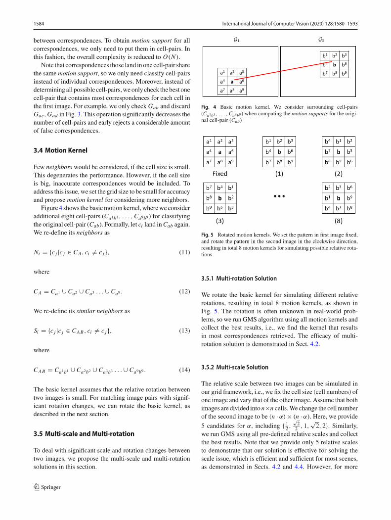
between correspondences. To obtain motion support for allcorrespondences, we only need to put them in cell-pairs. Inthis fashion, the overall complexity is reduced to O(N ).

Note that correspondences those land in one cell-pair sharethe same motion support, so we only need classify cell-pairsinstead of individual correspondences. Moreover, instead ofdetermining all possible cell-pairs,weonly check thebest onecell-pair that contains most correspondences for each cell inthe first image. For example, we only check Gab and discardGac,Gad in Fig. 3. This operation significantly decreases thenumber of cell-pairs and early rejects a considerable amountof false correspondences.

3.4 Motion Kernel

Few neighbors would be considered, if the cell size is small.This degenerates the performance. However, if the cell sizeis big, inaccurate correspondences would be included. Toaddress this issue, we set the grid size to be small for accuracyand propose motion kernel for considering more neighbors.

Figure 4 shows the basicmotion kernel,wherewe consideradditional eight cell-pairs (Ca1b1, . . . ,Ca9b9 ) for classifyingthe original cell-pair (Cab). Formally, let ci land inCab again.We re-define its neighbors as

Ni = {c j |c j ∈ CA, ci �= c j }, (11)

where

CA = Ca1 ∪ Ca2 ∪ Ca3 . . . ∪ Ca9 . (12)

We re-define its similar neighbors as

Si = {c j |c j ∈ CAB, ci �= c j }, (13)

where

CAB = Ca1b1 ∪ Ca2b2 ∪ Ca3b3 . . . ∪ Ca9b9 . (14)

The basic kernel assumes that the relative rotation betweentwo images is small. For matching image pairs with signif-icant rotation changes, we can rotate the basic kernel, asdescribed in the next section.

3.5 Multi-scale andMulti-rotation

To deal with significant scale and rotation changes betweentwo images, we propose the multi-scale and multi-rotationsolutions in this section.

G1 G2

a1 a2 a3

a4 a a6

a7 a8 a9

b1 b2 b3

b4 b b6

b7 b8 b9

Fig. 4 Basic motion kernel. We consider surrounding cell-pairs(Ca1b1 , . . . ,Ca9b9 ) when computing the motion supports for the origi-nal cell-pair (Cab)

Fig. 5 Rotated motion kernels. We set the pattern in first image fixed,and rotate the pattern in the second image in the clockwise direction,resulting in total 8 motion kernels for simulating possible relative rota-tions

3.5.1 Multi-rotation Solution

We rotate the basic kernel for simulating different relativerotations, resulting in total 8 motion kernels, as shown inFig. 5. The rotation is often unknown in real-world prob-lems, so we run GMS algorithm using all motion kernels andcollect the best results, i.e., we find the kernel that resultsin most correspondences retrieved. The efficacy of multi-rotation solution is demonstrated in Sect. 4.2.

3.5.2 Multi-scale Solution

The relative scale between two images can be simulated inour grid framework, i.e., we fix the cell size (cell numbers) ofone image and vary that of the other image. Assume that bothimages are divided inton×n cells.We change the cell numberof the second image to be (n · α) × (n · α). Here, we provide

5 candidates for α, including { 12 ,√22 , 1,

√2, 2}. Similarly,

we run GMS using all pre-defined relative scales and collectthe best results. Note that we provide only 5 relative scalesto demonstrate that our solution is effective for solving thescale issue, which is efficient and sufficient for most scenes,as demonstrated in Sects. 4.2 and 4.4. However, for more

123


significant scale changes, we can use more candidates orincrease α.

Algorithm 1 Grid-based Motion StatisticsInput: C, S, K {Correspondences, Scale, Kernel}Output: X {Selected Correspondences}G1,G2 = GenerateGrids(S); {Fig. 3}for all Ga ∈ G1 do

Find Gb from G2 with Gab having most matchesCA,CAB ,Cab = Search(K ,Gab); {Fig. 4, Fig. 5}τ = α

√|CA| − 1; {Eq. 8}s = |CAB | − 1; {Eq. 13}if s > τ then

X = X ∪ Cab;end if

end forShift the gird of the first image by half cell-width in horizontal, ver-tical, and both directions, and then repeat algorithm more 3 times.return X

3.6 Algorithm and Limitation

Algorithm 1 shows the GMS algorithm, which takes putativecorrespondences and the setting for scale and rotation as inputand outputs selectedmatches.We use the basicmotion kerneland the single equal scale for matching regular images, e.g.,video frames. The multi-scale and multi-rotation solutionsare used for images with significant changes in scale androtation, respectively.

3.6.1 Implementation

We implement the algorithms using C++ with OpenCVlibrary (Bradski 2000). A single CPU thread is used cur-rently, but the multi-thread programming can be used foraccelerating the multi-scale and multi-rotation solutions. Weuse 20×20 cells as the default mode, andwe vary the numberof cells in the second image when activating the multi-scalesolution. α = 4 in Eq. 8 is used for thresholding. The codehas been integrated into the OpenCV library.

3.6.2 Limitation

The limitation of GMS lies in three aspects. First, as weassume that image motion is piece-wise smooth, the per-formance may degenerate in areas where the assumption isviolated, e.g., image boundaries. This issue is not criticalbecause regular pixels are overwhelminglymore than bound-aries. Besides, as we are not targeting a final correspondencesolution but a set of high-quality hypotheses, the assumptionis sufficient for our purpose. To solve this problem, we willconsider using edge detection (Liu et al. 2019) or image seg-mentation (Cheng et al. 2016; Liu et al. 2018) techniques in

future work. Second, the performance is limited in visuallysimilar but geographically different image regions. This issueoften occurs in scenes that have heavy repetitive patterns.We leave the problem to global geometry estimation algo-rithms (Kushnir and Shimshoni 2014), as only local visualinformation is not sufficient to address that. Third, as we pro-cess data at the cell-pair level, inaccurate correspondencesthat lie the correct cell-pair will remain. These correspon-dences are useful inmany applicationswhich are not sensitiveto matching accuracy such as Object Retrieval (Philbin et al.2007). However, for accuracy-sensitive tasks, e.g., geometryestimation, they should be excluded. Therefore, we proposeto run GMS on correspondences selected by RT instead of allputative correspondences for mitigating the issue. The effi-cacy of using RT as pre-processing can be seen in Fig. 7 andTable 4.

4 Experiments

We evaluate four aspects of GMS:

– Comprehensive performance characterization on corre-spondence selection.

– Matching challenging image pairs with significant rela-tive scale and rotation changes.

– Contribution to the overall performance of featurematch-ing and epipolar geometry estimation.

– Integration in real-time computer vision applications, i.e.,Visual SLAM here.

4.1 GMS for Correspondence Selection

To comprehensively evaluate the performance of GMS, weexperiment with different local features and varying featurenumbers. We also examine the accuracy of retrieved corre-spondences using varying error thresholds. Two challengingdatasets (Graffiti and Wall) selected from VGG (Mikola-jczyk and Schmid 2005) are used for evaluation, which arewell-known for significant viewpoint changes. Each datasetcontains six images, where the ground truth homographybetween the first image to others is provided, resulting infive pairs with increasing difficulty for testing. Recall andPrecision are used as evaluation metrics, where we regardcorrespondences those distances to the ground truth aresmaller than 10 pixels as correct and others as wrong.

4.1.1 Results on Different Features

Figure 6 shows the results onGraffiti andWall datasets,whereSIFT (Lowe 2004) and ASIFT (Morel and Yu 2009) areused for generating correspondences, respectively. We testGMS on both all correspondences and the correspondences

123


(a)Graffiti (#SIFT=1741)

1 2 3 4 5Pairs

0

0.2

0.4

0.6

0.8

1

Rec

all

1 2 3 4 5Pairs

0

0.2

0.4

0.6

0.8

1

Pre

cisi

on

SIFT-RTSIFT-GMSSIFT-RT-GMS

(b)Graffiti (#ASIFT=31199)

1 2 3 4 5Pairs

0.2

0.4

0.6

0.8

1

Rec

all

1 2 3 4 5Pairs

0.85

0.9

0.95

1P

reci

sion

ASIFT-RTASIFT-GMSASIFT-RT-GMS

(c)Wall (#SIFT=2748)

1 2 3 4 5Pairs

0

0.2

0.4

0.6

0.8

1

Rec

all

1 2 3 4 5Pairs

0

0.2

0.4

0.6

0.8

1

Pre

cisi

on

SIFT-RTSIFT-GMSSIFT-RT-GMS

(d)Wall (#ASIFT=58049)

1 2 3 4 5Pairs

0.2

0.4

0.6

0.8

1

Rec

all

1 2 3 4 5Pairs

0.95

0.96

0.97

0.98

0.99

1

Pre

cisi

on

ASIFT-RTASIFT-GMSASIFT-RT-GMS

Fig. 6 Results on pairs with gradually increasing viewpoint changes.“#” stands for the feature numbers. RT refers to Lowe’s ratio test (Lowe2004). GMS and RT take all correspondences as input, while RT–GMStakes the results of RT as input. Therefore, the Recall of RT is the upperbound for RT–GMS

selected by Lowe’s ratio test. Here SIFT is not able to pro-vide sufficient correct correspondences on very challengingpairs due to significant viewpoint changes, while ASIFT can.The results show that GMS gets high recall and precision oncorrespondences generated byASIFT,while the recall degen-erates on correspondences generated by SIFT. The reason isthat ASIFT provide sufficient correspondences andGMS cantranslate the high feature numbers to high match quality, asindicated in Eq. 6, while SIFT correspondences are quitesparse. However, on SIFT correspondences, RT–GMS canachieve high performance, although they are sparse. Notethat the Recall of RT is the upper bound of RT–GMS. This

(a) SIFT

0 5 10 15Error Thresholds (px)

0.05

0.1

0.15

0.2

0.25

#Cor

rect

/ 87

05

AllRTGMSRT-GMS


0

0.2

0.4

0.6

0.8

1

Pre

cisi

on

(b) ASIFT


0

0.1

0.2

0.3

0.4

0.5

#Cor

rect

/ 15

5995


0

0.2

0.4

0.6

0.8

1

Pre

cisi

on

Fig. 7 Results with varying error thresholds on Graffiti. We collect allcorrespondences (ALL) in total 5 pairs for evaluation

is because the performance of GMS is also related to thefeature quality, as indicated in Eq. 6, and the quality ofcorrespondences selected by RT is higher than that of ini-tial correspondences in terms of precision. Compared withSIFT–RT, the most widely used feature matching method aswe know, the proposed SIFT–RT–GMS can get similar recall(i.e., similar correspondence numbers) but higher precision.It has important implications formany computer vision appli-cations. We show a comparison of both methods in Table 2,where the performance gap is wide on challenging wide-baseline datasets in terms of epipolar geometry estimation.

4.1.2 Accuracy of Correspondences

Figure 7 shows the results with varying error thresholds onGraffiti, whereweuse all correspondences inGraffiti (5 pairs)for evaluation. Note that regarding the number of correctcorrespondences, ALL is the upper bound for GMS, andRT is the upper bound for RT–GMS. The results show thatASIFT provides better correspondences than SIFT (see ALLfor comparison). However, when RT or GMS is applied, theprecision on SIFT correspondences is higher than that onASIFT correspondences, especially when the error thresholdis small, e.g., 1 or 2 pixels. This is because there aremany cor-rect but not accurate correspondences generated by ASIFTand selected by RT and GMS. These inaccurate correspon-dences are useful in many applications where the accuracyis not critical, e.g., Object Retrieval (Philbin et al. 2007).However, they limit the performance of accuracy-sensitiveapplications such as epipolar geometry estimation. There-fore, we suggest using SIFT–RT–GMS solution for highaccuracy of matching. Note that using ASIFT is also possible

123


(a) GMS

#100

#200

#500 #1

K

#2K

#5K

#10K

#20K

#50K

0

0.2

0.4

0.6

0.8

1

Rec

all

#100

#200

#500 #1

K

#2K

#5K

#10K

#20K

#50K

0

0.2

0.4

0.6

0.8

1

Pre

cisi

on

pair1pair2pair3pair4pair5

(b) RT

#100

#200

#500 #1

K

#2K

#5K

#10K

#20K

#50K

0

0.2

0.4

0.6

0.8

1

Rec

all

#100

#200

#500 #1

K

#2K

#5K

#10K

#20K

#50K

0

0.2

0.4

0.6

0.8

1P

reci

sion


(c) RT-GMS

#100

#200

#500 #1

K

#2K

#5K

#10K

#20K

#50K

0

0.2

0.4

0.6

0.8

1

Rec

all

#100

#200

#500 #1

K

#2K

#5K

#10K

#20K

#50K

0

0.2

0.4

0.6

0.8

1

Pre

cisi

on


Fig. 8 Results with varying maximum feature numbers on Graffitidataset. We randomly pick a subset of detected ASIFT features in eachimage for evaluation

and may lead to a higher performance, since ASIFT corre-spondences are generally better than SIFT correspondences.For example, Lin et al. (2017) uses ASIFT features andachieves the state-of-the-art performance in terms of cam-era pose estimation. However, it uses a highly complicatedregressionmethod,which consumes huge computational costto remove inaccurate correspondences.

4.1.3 Performance with Varying Feature Numbers

Equation 6 indicates that the performance of GMS relies onfeature numbers. To understand how feature numbers impactit, we randomly pick a subset of ASIFT features with varyingmaximum feature numbers for evaluation. Figure 8 showsthe results on Graffiti dataset. It shows that GMS requiresthe most features, while the performance of RT is less sen-sitive to feature numbers. RT-GMS can reduce the numberrequirement of GMS and achieves the most accurate match-ing. Overall, we suggest users trying RT and RT-GMS inscenarios where feature numbers are limited. Besides, notethat the performance of GMS is also related to feature qual-ity. We show that with the same feature detector (i.e., the

(a) Venice (Scale), #SIFT=3241

0 2 4 6Pairs

0

0.2

0.4

0.6

0.8

1

Rec

all

0 2 4 6Pairs

0

0.2

0.4

0.6

0.8

1

Pre

cisi

on

SIFT-RTSIFT-RT-GMSSIFT-RT-GMS-S

(b) Semper (Rotation), #SIFT=3257

0 2 4 6 8Pairs

0

0.2

0.4

0.6

0.8

1

Rec

all

0 2 4 6 8Pairs

0.85

0.9

0.95

1

Pre

cisi

on

SIFT-RTSIFT-RT-GMSSIFT-RT-GMS-R

(c) Boat (Scale+Rotation), #SIFT=2211

1 2 3 4 5Pairs

0

0.2

0.4

0.6

0.8

1

Rec

all

1 2 3 4 5Pairs

0.7

0.8

0.9

1

Pre

cisi

on

SIFT-RTSIFT-RT-GMSSIFT-RT-GMS-SR

Fig. 9 Robustness to scale and rotation change. GMS-S, GMS-R, andGMS-SR refer to our method with multi-scale, multi-rotation, and boththem, respectively

same feature numbers), using better descriptors could alsoimprove the performance in Sect. 4.4.

4.2 Robustness to Scale and Rotation Change

We use Semper and Venice datasets for testing the robust-ness ofGMS to rotation and scale changes, respectively. Bothdatasets are selected from Heinly et al. (2012), which is anextension of VGG (Mikolajczyk and Schmid 2005) with thesame data organization. We also use Boat dataset for test-ing, where image pairs have significant relative changes inboth scale and rotation. Figure 9 shows the results, wherewe use SIFT feature (Lowe 2004) for generating putativecorrespondences and run GMS variants on correspondencesselected by RT. It shows that the basic GMS is sensitive tolarge scale and rotation changes while using the multi-scaleandmulti-rotation solution can improve the performance sig-nificantly. Similar to previous results, the proposed methodcan achieve similar recall with RT and higher precision. Weshow visual results of GMS in Fig. 10, where the results onthe most challenging pair of each dataset is illustrated. Thescale invariance is critical in the unstructured environment, as

123


Graffiti

Venice

Semper

(a) ASIFT-RT-GMS on

(b) SIFT-RT-GMS-S on

(c) SIFT-RT-GMS-R on

(d) SIFT-RT-GMS-SR on Boat

Fig. 10 Visual results of GMS. We show matching results on the mostchallenging pair of each dataset, where at most 100 correspondencesare plotted for clear visualization

the relative scale of images is unknown. We show that usingthe proposed multi-scale solution can significantly improvethe performance for challenging wide-baseline scenarios inTable 4.

4.3 Runtime of GMS

We evaluate the runtime of GMS with varying feature num-bers on Graffiti dataset using ASIFT features. Figure 11shows the results, where GMS takes about only 2ms in a sin-gle CPU thread, even when feature numbers reach 50, 000.The multi-scale (GMS-S) and multi-rotation (GMS-R) vari-ants repeat the basic GMSwith different pre-defined patterns5 and 8 times, respectively. Therefore, their computationalcosts are linearly increased. We do not show GMS-SR in the

#100

#200

#500 #1

K

#2K

#5K

#10K

#20K

#50K

0

2

4

6

8

10

12

14

16

18

mill

isec

onds

GMS

GMS-S

GMS-R

Fig. 11 Runtime of GMS in a single CPU thread. GMS-S and GMS-Rrepeat the basicGMSusing different settings 5 and 8 times, respectively,so the runtime is linearly increased. GMS-SR, not shown in this figure,consumes 40 times more computational cost than the basic GMS. Notethat the multi-scale andmulti-rotation solutions could be accelerated byusing multi-threshold programming, since no data dependence exists indifferent repeats

figure for clarity. However, its time consuming is apparent,i.e., 40 times higher than the basicGMS.Note that bothmulti-scale and multi-rotation solutions have no data-dependentin different repeats, so they could be accelerated by usingmulti-thread programming. Theoretically, the multi-scale (orrotation) version could achieve the same speed with the basicGMS, when there are 5 (or 8) CPU threads available.

4.4 GMS for Epipolar Geometry Estimation

We evaluate the proposed method on FM-Bench (Bian et al.2019), where correspondences selection methods are inte-grated into a classic feature matching and epipolar geometryestimation pipeline (i.e., SIFT, RANSAC, and the 8-pointalgorithm), and the overall performance is compared. Thebenchmark datasets, metrics, and baselines are describedbelow.

4.4.1 Datasets

FM-Bench consists of 4 datasets, including TUM (Sturmet al. 2012), KITTI (Geiger and Lenz 2012), Tanks and Tem-ples (T&T) (Knapitsch et al. 2017), and a Community PhotoCollection (CPC) dataset (Wilson and Snavely 2014). Thefirst two datasets are popular for Visual SLAM testing, whichprovide indoor and outdoor videos, respectively. The last twodatasets are widely used for structure-from-motion evalua-tion, which provides wide-baseline scenarios. Especially, the

123


Table 1 Details of thebenchmark dataset

Datasets #Seq #Images Resolution Baseline Property

TUM 3 5994 480 × 640 Short Indoor scenes

KITTI 5 9065 370 × 1226 Short Street views

T&T 3 922 1080 × 2048 Wide Outdoor scenes

1080 × 1920

CPC 1 1615 Varying Wide Internet images

Fig. 12 Sample images of the benchmark datasets

CPC dataset is challenging, in which images are collectedfrom the Internet and captured by tourists. 1000 matchingimage pairs per dataset are randomly picked by Bian et al.(2019) for testing. Table 1 summarizes the test dataset, andFig. 12 shows sample images.

4.4.2 Baselines

We compare with three state-of-the-art correspondenceselection methods, including CODE (Lin et al. 2017),LPM (Ma et al. 2019), LC (Yi et al. 2018) as strong baselines.CODE leverages the sophisticated non-linear optimizationfor finding correct correspondences, and it relies on a self-implemented GPU-ASIFT feature, which extracts severaltimes more features than the standard ASIFT (Morel and Yu2009). LPM explores neighborhood structures, and LC usesdeeply trained neural networks. Both methods are indepen-dent of features and use SIFT (Lowe 2004) in the originalpaper. Note that the comparison is unfair to our methodbecause CODE uses ASIFT features and a very complicatedsolution (1000× slower than GMS).

4.4.3 Implementation Details

We use the DoG detector and SIFT descriptor (Lowe 2004)for generating putative correspondences. The implementa-tion is from theVLFeat library (Vedaldi andFulkerson 2010).We use the default parameters, which results in average 1082,1751, 8133, and 7213 detected features in four datasets (asorder in Fig. 12). The correspondences are pre-processed byusing ratio test (RT), with the threshold being 0.8. Then weapply the evaluate methods (LPM, LC, and GMS) for goodcorrespondence selection.We empirically find that using cor-respondences by RT results in better performance than using

Table 2 %Recall of fundamental matrix estimation

Method Dataset

TUM KITTI T&T CPC

CODE 62.50 92.50 89.40 51.00

SIFT–RT 57.40 91.70 70.00 29.20

SIFT–RT–LPM 58.90 91.50 80.70 39.40

SIFT–RT–LC 54.10 89.70 76.60 39.40

SIFT–RT–GMS 59.20 91.70 80.90 43.00

Bold values indicate the best performance

all correspondences for LC (Yi et al. 2018), although it usesthe latter in the original paper. We use the basic GMS inthe first two SLAM datasets and the multi-scale solutionin the last two SfM datasets, as where images are moreunstructured. The multi-rotation solution is not used sincethere is no significant image rotation in these datasets. ForCODE (Lin et al. 2017), we directly evaluate the output cor-respondences since it is a highly integrated correspondencesystem. We use the publicly available implementation forall methods and use the pre-trained model by authors forLC.

4.4.4 Metrics

To compare the overall performance of different corre-spondence systems, we fed their correspondences into aRANSAC-based 8-point estimator (Fischler and Bolles1981; Hartley 1997) to recover the FM, and then comparethe estimated FM with the ground truth FM using normal-ized symmetric geometry distance (NSGD) (Bian et al. 2019).See the appendix for details. We then report the success ratioof FM estimation (%Recall), where the NSGD threshold is0.05, and we also show the results with varying error thresh-olds. What’s more, we report the inlier rate (%Inlier) afterRANSAC-based outlier removal for match quality compar-ison. Here inliers refer to matches those distances to theground truth epipolar lines are smaller than α ∗ l, where lstands for the length of image diagonal and α = 0.003.More details can be found in the appendix and Bian et al.(2019).

123


(a) T&T

Normlized SGD Threshold

0

10

20

30

40

50

60

70

80

90

100

%R

ecal

l

SIFT-RT

SIFT-RT-LPM

SIFT-RT-LC

SIFT-RT-GMS

CODE

(b) CPC

0 0.05 0.1 0.15 0.2

0 0.05 0.1 0.15 0.2

Normlized SGD Threshold

0

10

20

30

40

50

60

70

80

90

100

%R

ecal

l

SIFT-RT

SIFT-RT-LPM

SIFT-RT-LC

SIFT-RT-GMS

CODE

Fig. 13 FMestimation onwide-baseline datasets. GMScan outperformrecent LC and LPM using the same feature correspondences as input

4.4.5 Experimental Results

Table 2 shows the recall of FM estimation. Figure 13 showsthe resultswith varying error thresholds on twowide-baselinedatasets. Table 3 reports the inlier rate. All the above resultsdemonstrate that GMS can show better performance withLC (Yi et al. 2018) and LPM (Ma et al. 2019) using thesame feature correspondences as input, i.e., SIFT–RT (Lowe2004). However, our correspondence system is not as good asthe powerful CODE (Lin et al. 2017) system. Compares withSIFT–RT, our approach can lead to significantly better resultson T&T and CPC datasets, demonstrating the efficacy of

Table 3 %Inlier of correspondences after RANSAC

Method Dataset

TUM KITTI T&T CPC

CODE 76.95 98.32 89.14 90.16

SIFT–RT 75.33 98.20 75.20 67.14

SIFT–RT–LPM 75.75 98.27 81.62 78.17

SIFT–RT–LC 75.96 99.44 84.01 83.99

SIFT–RT–GMS 76.18 98.58 84.38 85.90


Table 4 Ablation study results (FM %Recall) for the multi-scale solu-tion and RT pre-processing

Method Dataset

TUM KITTI T&T CPC

SIFT–RT–GMS 59.20 91.70 80.90 43.00

Without RT 51.9 90.6 73.4 31.4

Without multi-scale X X 78.6 37.8


Table 5 Results (FM %Recall) of GMS with deep learning based fea-tures

Method Dataset

TUM KITTI T&T CPC

CODE 67.50 91.90 92.70 61.80

DoG–HardNet–RT–GMS 68.60 92.10 92.20 60.10

HesAff–HardNet–RT–GMS 66.40 91.80 90.90 60.80

Bold and italics denote the first and second performance, respectively

GMS for high-accuracy matching. Concerning the runtime,CODE requires several seconds for correspondence selec-tion, while GMS is more 1000 times faster. As the authorsreported, LC needs 13ms on GPU (or 25ms on CPU) tofind good correspondences from 2K putative matches, andLPM can identify false matches from 1000 putative corre-spondences in a few milliseconds. They are both slower thanthe proposed method (Fig. 11).

4.4.6 Effects of RT andMulti-scale

To understand how our multi-scale solution and using RTbefore GMS can benefit the overall performance, we conductan ablation study by removing them respectively. The resultsare shown in Table 4. It shows that the performance is signif-icantly decreased without RT. The reason is that inaccuratecorrespondences are included, and they limit the performanceof geometry estimation. Besides, the results onwide-baselinematching datasets (T&TandCPC) demonstrate that using theproposed multi-scale solution can significantly improve theperformance.

123


Table 6 Monocular SLAMinitialization results on theKITTI odometrydataset

Seq Frag Success ratio Orders #3D pointsORB GMS ORB GMS ORB GMS

00 227 0.77 0.95 2.8 1.18 140.44 929.59

01 55 0.11 0.80 4.16 3.88 119.00 519.77

02 233 0.73 0.98 4.28 1.14 124.28 858.01

03 40 0.78 0.98 2.77 1.28 136.97 881.74

04 13 0.69 0.92 6.78 1.08 123.11 875.00

05 138 0.80 0.95 2.65 1.38 132.99 848.60

06 55 0.70 0.96 5.13 1.38 116.62 704.24

07 55 0.73 0.87 2.0 1.31 133.33 882.92

08 203 0.66 0.96 3.65 1.23 126.69 786.53

09 79 0.65 0.98 3.39 1.24 129.94 790.01

10 60 0.75 0.98 5.31 1.32 122.00 843.56

4.4.7 Paring with Deep Features

As Eq. 6 indicates that the performance of GMS is related tofeature quality, we experiment with recently proposed deeplearning based features, including the HardNet (Mishchuket al. 2017) descriptor and HessAff (Mishkin et al. 2018)detector. Specifically, we use DoG (Lowe 2004) and Hes-sAff for interest point detection, respectively. Then we useuseHardNet to compute descriptors, resulting in two putativecorrespondence generation solutions. The powerful CODEis compared as the strong baseline. Instead of RANSAC, weuse LMedS (Rousseeuw and Leroy 1987) based FM esti-mator here, as it shows better performance than the formerin FM-Bench (Bian et al. 2019). Table 5 shows the results,where GMS with deep features can achieve a competitiveperformance with CODE (Lin et al. 2017). The results areremarkable and have important implications to real-timeapplications since these deep features are efficient, whileCODE is several orders of magnitude slower.

4.5 GMS for Monocular SLAM Initialization

Monocular SLAM methods (Mur-Artal et al. 2015) have toinitialize the system before tracking and mapping, where theinitial 3D map is created by triangulating correspondencesto recover depths. Robust initialization has important impli-cations for a monocular SLAM system, and high-qualitycorrespondence is the key to this step. As Visual SLAMsystems have high requirements for the run-time of meth-ods for the overall real-time performance, many advancedcorrespondence approaches can not be used in this scenario.Fortunately, GMS is sufficiently fast for this purpose. In thissection, we show that GMS can be used in the popular ORB-SLAMsystem (Mur-Artal et al. 2015) for better initialization.

4.5.1 Integration

In the initializer of ORB-SLAM, we replace the originalBag-of-Words based matching with the brute-force nearestneighbor matching, and we apply GMS for selecting goodcorrespondences. The selected matches are used to recovergeometry and create the 3Dmap by triangulation. For systemstability, we use the default feature detection parameters, i.e.,detecting 4K well-distributed ORB features for initializationin KITTI-like images.

4.5.2 Dataset and Metrics

Weevaluatemethods on the sequence 00–10 ofKITTI odom-etry dataset (Geiger and Lenz 2012). For each sequence, wecrop it into non-overlap fragments, with each fragment con-taining 20 consecutive frames. The performance averagedover all fragments is reported In each fragment, we measure(1) whether the initialization is successful; (2) how quicklythe system is initialized; and (3) how many 3D points aregenerated. Regarding (1), we compare the estimated cam-era pose with the ground truth, and those are recognized assuccessful if pose error is less than 5 degrees in both rotationand translation. Regarding (2), we report the order of the firstsuccessfully initialized image in each fragment.

4.5.3 Experimental Results

Table 6 shows the results, where we compare with the orig-inal initializer. It shows that the proposed initializer leadsto a significantly higher success ratio, faster initialization,and denser 3D map. This has a huge impact on monocularSLAM systems, especially when they work on challengingenvironments where previous solutions fail to provide reli-able correspondences for initialization. The proposedmethodcan mitigate this issue and enable the use of SLAM systemsin more real-world scenarios.

5 Conclusion

This paper presents a fast correspondence selection algorithmthat we termed grid-based motion statistics (GMS). It caneffectively separate true correspondences from false ones athigh speed by leveraging the motion smoothness constraint.Comprehensive experimental results demonstrate its robust-ness in different environments.We also show that it advancesthe feature matching and geometry estimation. Moreover,we plug GMS into the Monocular ORB-SLAM system forinitialization, demonstrating its great potential to real-timeapplications. The code has been released and integrated intothe OpenCV library.

123


Acknowledgements This work was supported by Australian Centre ofExcellence for Robotic Vision CE140100016, and the ARC LaureateFellowship FL130100102 to Prof. Ian Reid. This work was supportedby Major Project for New Generation of AI (No. 2018AAA0100403),NSFC (61922046), and Tianjin Natural Science Foundation (No.18JCYBJC41300 and No. 18ZXZNGX00110) to Prof. Ming-MingCheng. This work was supported by the Singapore Ministry of Edu-cation (MOE) Academic Research Fund (AcRF) Tier 1 grant to Prof.Wen-Yan Lin. This work was supported by the Singapore MOE Aca-demic Research Fund MOE2016-T2-2-154, and an internal grant fromHKUST (R9429) to Prof. Sai-Kit Yeung. Besides, the authors thankProf. Yasuyuki Matsushita for his contribution in the early stage of thispaper.

Open Access This article is licensed under a Creative CommonsAttribution 4.0 International License, which permits use, sharing, adap-tation, distribution and reproduction in any medium or format, aslong as you give appropriate credit to the original author(s) and thesource, provide a link to the Creative Commons licence, and indi-cate if changes were made. The images or other third party materialin this article are included in the article’s Creative Commons licence,unless indicated otherwise in a credit line to the material. If materialis not included in the article’s Creative Commons licence and yourintended use is not permitted by statutory regulation or exceeds thepermitted use, youwill need to obtain permission directly from the copy-right holder. To view a copy of this licence, visit http://creativecommons.org/licenses/by/4.0/.

Appendix

Normalized SGD

We use the NSGD (Bian et al. 2019) to measure the geo-metric distance between two fundamental matrices (FMs),which is an extension of the SGD error (Zhang 1998). Themethod generates virtual correspondences using two mod-els, and crossly computes the distance of correspondence tothe epipolar line generated by the other model. The resultsare symmetrical, i.e., the error from F1 to F2 is equal to theerror from F2 to F1. For generalization in different resolutionimages, we rescale the error to the range (0, 1) by dividingthe length of image diagonal.

FM Ground Truth

The fundamental matrix between an image pair can bederived from the camera intrinsic and extrinsic parameters.The ground-truth camera parameters are provided in TUMand KITTI datasets, while they are unknown in T&T andCPC datasets. We derive ground-truth camera parametersfor the latter by reconstructing image sequences using theCOLMAP (Schonberger and Frahm 2016) library, as in Yiet al. (2018), Ranftl and Koltun (2018). Note that the SfMpipeline reasons globally about the consistency of 3D pointsand cameras, leading to accurate estimates with an averagereprojection error below one pixel.

References

Bian, J., Lin, W.-Y., Matsushita, Y., Yeung, S.-K., Nguyen, T. D., &Cheng, M.-M. (2017). GMS: Grid-based motion statistics for fast,ultra-robust feature correspondence. In IEEE conference on com-puter vision and pattern recognition (CVPR) (pp. 4181–4190).IEEE.

Bian, J.-W.,Wu, Y.-H., Zhao, J., Liu, Y., Zhang, L., Cheng,M.-M., et al.(2019). An evaluation of feature matchers for fundamental matrixestimation. In British machine vision conference (BMVC).

Bradski, G. (2000). The OpenCV library. Dr. Dobb’s Journal of Soft-ware Tools.

Breiman, L. (2001). Random forests. Machine Learning, 45(1), 5–32.Causo, A., Chong, Z.-H., Luxman, R., Kok, Y. Y., Yi, Z., Pang, W.-C.,

et al. (2018). A robust robot design for item picking. In 2018 IEEEinternational conference on robotics and automation (ICRA) (pp.7421–7426). IEEE

Cheng,M.-M.,Liu,Y.,Hou,Q.,Bian, J., Torr, P.,Hu, S.-M., et al. (2016).HFS: Hierarchical feature selection for efficient image segmenta-tion. In European conference on computer vision (ECCV) (pp.867–882). Springer.

Davison, A. J., Reid, I. D., Molton, N. D., & Stasse, O. (2007).Monoslam: Real-time single camera slam. IEEE Transactions onPattern Recognition and Machine Intelligence, 29(6), 1052–1067.

Fischler, M. A., & Bolles, R. C. (1981). Random sample consensus:A paradigm for model fitting with applications to image analysisand automated cartography. Communications of the ACM, 24(6),381–395.

Geiger,A., Lenz, P.,&Urtasun,R. (2012).Arewe ready for autonomousdriving? the kitti vision benchmark suite. In IEEE conference oncomputer vision and pattern recognition (CVPR) (pp. 3354–3361).IEEE.

Harris, C., & Stephens, M. (1988). A combined corner and edge detec-tor. In Alvey vision conference (pp. 10–5244).

Hartley, R. I. (1997). In defense of the eight-point algorithm. IEEETransactions on Pattern Recognition and Machine Intelligence,19(6), 580–593.

Heinly, J., Dunn, E., & Frahm, J.-M. (2012). Comparative Evaluationof Binary Features. In European conference on computer vision(ECCV) (pp. 759–773).

Knapitsch, A., Park, J., Zhou, Q.-Y., & Koltun, V. (2017). Tanks andTemples: Benchmarking large-scale scene reconstruction. ACMTransactions on Graphics, 36(4), 78.

Kushnir, M., & Shimshoni, I. (2014). Epipolar geometry estimation forurban scenes with repetitive structures. IEEE Transactions on Pat-tern Recognition and Machine Intelligence, 36(12), 2381–2395.

Lin, W.-Y., Lai, J.-H., Liu, S., & Matsushita, Y. (2018). Dimension-ality’s blessing: Clustering images by underlying distribution. InProceedings of the IEEE conference on computer vision and pat-tern recognition (pp. 5784–5793).

Lin, W.-Y., Wang, F., Cheng, M.-M., Yeung, S.-K., Torr, P. H., Do, M.N., et al. (2017). Code: Coherence based decision boundaries forfeature correspondence. IEEE Transactions on Pattern Recogni-tion and Machine Intelligence, 40(1), 34–47.

Liu, Y., Cheng, M.-M., Hu, X., Bian, J.-W., Zhang, L., Bai, X., et al.(2019). Richer convolutional features for edge detection. IEEETransactions on Pattern Recognition and Machine Intelligence,41(8), 1939–1946.

Liu, Y., Jiang, P.-T., Petrosyan, V., Li, S.-J., Bian, J., Zhang, L.,et al. (2018). DEL: Deep embedding learning for efficient imagesegmentation. In International joint conference on artificial intel-ligence (IJCAI).

Liu, Z., & Marlet, R. (2012). Virtual line descriptor and semi-localmatching method for reliable feature correspondence. In Britishmachine vision conference (BMVC) (pp. 16–1).

123

http://creativecommons.org/licenses/by/4.0/

http://creativecommons.org/licenses/by/4.0/


Lowe, D. G. (2004). Distinctive image features from scale-invariantkeypoints. International Journal on Computer Vision, 60(2), 91–110.

Ma, J., Zhao, J., Jiang, J., Zhou, H., &Guo, X. (2019). Locality preserv-ing matching. International Journal on Computer Vision, 127(5),512–531.

Ma, J., Zhao, J., Tian, J., Yuille, A. L., & Tu, Z. (2014). Robust pointmatching via vector field consensus. IEEE Transactions on ImageProcessing, 23(4), 1706–1721.

Mikolajczyk, K., & Schmid, C. (2005). A performance evaluation oflocal descriptors. IEEE Transactions on Pattern Recognition andMachine Intelligence, 27(10), 1615–1630.

Mishchuk, A., Mishkin, D., Radenovic, F., &Matas, J. (2017).Workinghard to know your neighbor’s margins: Local descriptor learningloss. In Neural information processing systems (NIPS) (pp. 4826–4837).

Mishkin, D., Radenovic, F., & Matas, J. (2018). Repeatability is notenough: Learning affine regions via discriminability. In Europeanconference on computer vision (ECCV) (pp. 284–300). Springer.

Morel, J.-M., & Yu, G. (2009). Asift: A new framework for fully affineinvariant image comparison. SIAM Journal on Imaging Sciences,2(2), 438–469.

Muja, M., & Lowe, D. G. (2009). Fast approximate nearest neighborswith automatic algorithm configuration. VISAPP (1), 2(331–340),2.

Mur-Artal, R., Montiel, J. M. M., & Tardos, J. D. (2015). ORB-SLAM:A versatile and accurate monocular slam system. IEEE Transac-tions on Robotics, 31(5), 1147–1163.

Philbin, J., Chum, O., Isard, M., Sivic, J., & Zisserman, A. (2007).Object retrieval with large vocabularies and fast spatial matching.In IEEE conference on computer vision and pattern recognition(CVPR) (pp. 1–8). IEEE.

Ranftl, R., &Koltun, V. (2018). Deep fundamental matrix estimation. InEuropean conference on computer vision (ECCV) (pp. 284–299).

Rousseeuw, P. J., & Leroy, A. M. (1987). Robust regression and outlierdetection (Vol. 589). New York: wiley.

Rublee, E., Rabaud, V., Konolige, K., & Bradski, G. (2011). ORB: Anefficient alternative to sift or surf. In IEEE international conferenceon computer vision (ICCV) (pp. 2564–2571). IEEE.

Schonberger, J. L., & Frahm, J.-M. (2016). Structure-from-motionrevisited. In IEEE conference on computer vision and patternrecognition (CVPR) (pp. 4104–4113).

Sturm, J., Engelhard, N., Endres, F., Burgard,W.,&Cremers, D. (2012).A benchmark for the evaluation of RGB-d slam systems. In IEEEinternational conference on intelligent robots and systems (IROS)(pp. 573–580). IEEE.

Vedaldi, A., & Fulkerson, B. (2010). VLFeat: An open and portablelibrary of computer vision algorithms. In ACM international con-ference on multimedia (ACM MM) (pp. 1469–1472). ACM.

Wilson, K., & Snavely, N. (2014). Robust global translations with1DSFM. In European conference on computer vision (ECCV) (pp.61–75). Springer.

Yi, K. M., Trulls, E., Ono, Y., Lepetit, V., Salzmann, M., & Fua, P.(2018). Learning to find good correspondences. In IEEE confer-ence on computer vision and pattern recognition (CVPR) (pp.2666–2674).

Yoon, J. S., Li, Z., & Park, H. S. (2018). 3D semantic trajectoryreconstruction from 3D pixel continuum. In IEEE conference oncomputer vision and pattern recognition (CVPR) (pp. 5060–5069).

Zhang, H., Hasith, K., & Wang, H. (2019). GMC: Grid based motionclustering in dynamic environment. In Proceedings of SAI intelli-gent systems conference (pp. 1267-1280). Springer, Cham.

Zhang, Z. (1998). Determining the epipolar geometry and its uncer-tainty: A review. International Journal on Computer Vision, 27(2),161–195.

Publisher’s Note Springer Nature remains neutral with regard to juris-dictional claims in published maps and institutional affiliations.

123

gms: grid-based motion statistics for fast, ultra-robust ...gms is robust to various challenging...

Documents