gnss signal demodulation performance in urban environments - gnss... · gnss signal demodulation...
TRANSCRIPT

HAL Id: hal-01158734https://hal-enac.archives-ouvertes.fr/hal-01158734
Submitted on 1 Jun 2015
HAL is a multi-disciplinary open accessarchive for the deposit and dissemination of sci-entific research documents, whether they are pub-lished or not. The documents may come fromteaching and research institutions in France orabroad, or from public or private research centers.
L’archive ouverte pluridisciplinaire HAL, estdestinée au dépôt et à la diffusion de documentsscientifiques de niveau recherche, publiés ou non,émanant des établissements d’enseignement et derecherche français ou étrangers, des laboratoirespublics ou privés.
GNSS Signal Demodulation Performance in UrbanEnvironments
Marion Roudier, Thomas Grelier, Lionel Ries, Axel Javier Garcia Peña,Olivier Julien, Charly Poulliat, Marie-Laure Boucheret, Damien Kubrak
To cite this version:Marion Roudier, Thomas Grelier, Lionel Ries, Axel Javier Garcia Peña, Olivier Julien, et al.. GNSSSignal Demodulation Performance in Urban Environments. 6th European Workshop on GNSS Signalsand Signal Processing, Dec 2013, Neubiberg, Germany. <hal-01158734>

GNSS Signal Demodulation Performance in Urban
Environments
Marion Roudier, Thomas Grelier, Lionel Ries
Radionavigation Signals and Equipments
CNES
Toulouse, France
[email protected], [email protected],
Charly Poulliat, Marie-Laure Boucheret
INPT-ENSEEIHT/IRIT
University of Toulouse
Toulouse, France
[email protected], Marie-
Axel Garcia-Pena, Olivier Julien
SIGNAV Research Group
ENAC
Toulouse, France
[email protected], [email protected]
Damien Kubrak
Thales Alenia Space
Toulouse, France
Abstract— Satellite navigation signals demodulation
performance is historically tested and compared in the Additive
White Gaussian Noise propagation channel model which well
simulates open areas. Nowadays, the majority of new applications
targets dynamic users in urban environments; therefore the
implementation of a simulation tool able to provide realistically
GNSS signal demodulation performance in obstructed
propagation channels has become mandatory. This paper
presents the simulator SiGMeP (Simulator for GNSS Message
Performance) which is wanted to provide demodulation
performance of any GNSS signals in urban environment, as
faithfully of reality as possible. The demodulation performance of
GPS L1C/A, GPS L2C, GPS L1C and Galileo E1 OS signals
simulated with SiGMeP in the AWGN channel model
configuration is firstly showed. Then, the demodulation
performance of GPS L1C simulated with SiGMeP in urban
environments is presented using the Prieto channel model with
two signal carrier phase estimation configurations: perfect signal
carrier phase estimation and PLL tracking.
Keywords— GNSS; demodulation performance; Clock and
Ephemeris Data; channel model; Land Mobile Satellite; statistical
propagation model; narrowband propagation; urban
I. INTRODUCTION
Global Navigation Satellite Systems (GNSS) are increasingly present in our everyday life. The interest of new users with further operational needs implies a constant evolution of the current GNSS systems. A significant part of the new applications are found in environments with difficult reception conditions such as urban or indoor areas. In these obstructed environments, the received signal is severely impacted by obstacles which generate fast variations of the received signal’s phase and amplitude that are detrimental to both the ranging and demodulation capability of the receiver. One option to deal with these constraints is to consider
enhancements to the current GNSS systems, where the design of an innovative signal more robust than the existing ones to distortions due to urban environments is one of the main aspects to be pursued. A research axis to make a signal more robust, which was already explored, is the design of new modulations adapted to GNSS needs that allows better ranging capabilities even in difficult environments [1][2]. However, other interesting axes remain to be fully explored such as the channel coding of the transmitted useful information: users could access the message content even when the signal reception is difficult.
Computer simulations based on realistic received signal models are widely used in order to provide a first strong validation of the demodulation performance of the newly designed signal. The aim of this paper is to provide and validate a software simulation tool, and to deliver first results. The simulator is referred to as Simulator for GNSS Message Performance (SiGMeP), able to compute the demodulation performance of any GNSS signals in a realistic urban Land Mobile Satellite (LMS) channel model.
The paper is organized as follows. Section II describes the propagation channel model used in the simulation tool SiGMeP. Section III presents the SiGMeP structure and suggests a validation process of the tool comparing simulated demodulation performance obtained with SiGMeP to results presented in [3] and [4]. Section IV provides refined demodulation performance for GPS L1C taking into account the impact of the Phase-Locked Loop (PLL) on the signal carrier phase estimation process, which is crucial in an urban environment to have relevant results.
II. URBAN LMS CHANNEL MODEL
The propagation channel, a LMS channel in urban environment, is the key element of the simulation which has to
be mathematically modeled. A LMS channel model state-of-the-art analysis shows that one model is mostly used for GNSS performance simulations: the model designed by F. Perez-Fontan in the early 2000 [5] [6] and improved by R. Prieto-Cerdeira in 2010 [7].
A. The Perez-Fontan Model Base
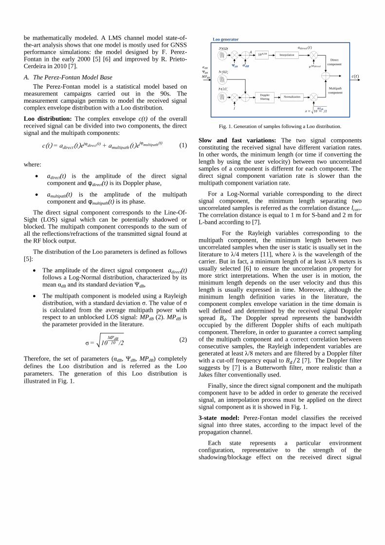
The Perez-Fontan model is a statistical model based on measurement campaigns carried out in the 90s. The measurement campaign permits to model the received signal complex envelope distribution with a Loo distribution.
Loo distribution: The complex envelope c(t) of the overall received signal can be divided into two components, the direct signal and the multipath components:
( ) ( ) ( )
(1)
where:
adirect(t) is the amplitude of the direct signal component and φdirect(t) is its Doppler phase,
amultipath(t) is the amplitude of the multipath component and φmultipath(t) is its phase.
The direct signal component corresponds to the Line-Of-Sight (LOS) signal which can be potentially shadowed or blocked. The multipath component corresponds to the sum of all the reflections/refractions of the transmitted signal found at the RF block output.
The distribution of the Loo parameters is defined as follows [5]:
The amplitude of the direct signal component adirect(t) follows a Log-Normal distribution, characterized by its mean αdB and its standard deviation ΨdB,
The multipath component is modeled using a Rayleigh distribution, with a standard deviation σ. The value of σ is calculated from the average multipath power with respect to an unblocked LOS signal: MPdB (2). MPdB is the parameter provided in the literature.
σ √
(2)
Therefore, the set of parameters (αdB, ΨdB, MPdB) completely
defines the Loo distribution and is referred as the Loo
parameters. The generation of this Loo distribution is
illustrated in Fig. 1.
Fig. 1. Generation of samples following a Loo distribution.
Slow and fast variations: The two signal components constituting the received signal have different variation rates. In other words, the minimum length (or time if converting the length by using the user velocity) between two uncorrelated samples of a component is different for each component. The direct signal component variation rate is slower than the multipath component variation rate.
For a Log-Normal variable corresponding to the direct signal component, the minimum length separating two uncorrelated samples is referred as the correlation distance lcorr. The correlation distance is equal to 1 m for S-band and 2 m for L-band according to [7].
For the Rayleigh variables corresponding to the multipath component, the minimum length between two uncorrelated samples when the user is static is usually set in the literature to λ/4 meters [11], where λ is the wavelength of the carrier. But in fact, a minimum length of at least λ/8 meters is usually selected [6] to ensure the uncorrelation property for more strict interpretations. When the user is in motion, the minimum length depends on the user velocity and thus this length is usually expressed in time. Moreover, although the minimum length definition varies in the literature, the component complex envelope variation in the time domain is well defined and determined by the received signal Doppler spread Bd. The Doppler spread represents the bandwidth occupied by the different Doppler shifts of each multipath component. Therefore, in order to guarantee a correct sampling of the multipath component and a correct correlation between consecutive samples, the Rayleigh independent variables are generated at least λ/8 meters and are filtered by a Doppler filter with a cut-off frequency equal to ⁄ [7]. The Doppler filter suggests by [7] is a Butterworth filter, more realistic than a Jakes filter conventionally used.
Finally, since the direct signal component and the multipath component have to be added in order to generate the received signal, an interpolation process must be applied on the direct signal component as it is showed in Fig. 1.
3-state model: Perez-Fontan model classifies the received signal into three states, according to the impact level of the propagation channel.
Each state represents a particular environment configuration, representative to the strength of the shadowing/blockage effect on the received direct signal
Loo generator
( )
Multipath
component
Direct
component
j
Doppler
filtering
√
Normalization
Interpolation
( )

component. The first state corresponds to LOS visibility conditions, the second state to a moderate shadowing and the third state to a deep shadowing. Therefore, each state has associated a different set of Loo parameters for a fixed satellite elevation.
The state changes are very slow because they represent the transition between two different obstacles [5]. The state frame length lframe corresponds to the average of the state length, in the order of 3-5 meters [6].
The state transitions are dictated by a first-order Markov chain [6], defined by the state transition probability matrix P (see Fig. 2).
Fig. 2. First-order Markov chain state transitions process.
B. An Evolution of the Perez-Fontan model: the Prieto Model
The Perez-Fontan 3-state model presents some limitations which involve a mismatch with reality. R. Prieto-Cerdeira proposes an evolution of the Perez-Fontan model, using it as a baseline. The same ensemble of measured data which was used by Perez-Fontan has been reanalysed, considering new assumptions:
A classification in two states instead of three for the Perez Fontan model, and
Loo parameters defined by random variables instead of constant values as for the Perez-Fontan model.
The mathematical model core is thus similar but two major differences appear.
2-state model: In the Prieto model, environmental conditions are classified in two states instead of the three of the Perez Fontan model:
“Good” for LOS to moderate shadowing, and
“Bad” for moderate to deep shadowing.
These two states represent two different macroscopic shadowing/blockage behaviour [7].
The state transitions are dictated by a semi-Markov model: the state changes are not anymore ruled by transition probabilities, we directly move from one state to the other (see Fig. 3).
The duration of each state is defined by a statistical law. Reference [7] suggests that the duration of each state follows a Log-Normal distribution, whatever the state Good or
Bad. The parameters of the Log-Normal distribution depend on the propagation environment. The database used in this paper to determine the Log-Normal parameters has been extracted from [7].
Fig. 3. Semi-Markov chain state transitions process.
Loo parameters generation: To compensate the reduction in the number of states (from three to two), both states of the Prieto model are allowed to take up a wide range of possible parameters values, compared to the Perez-Fontan model for which the parameters values were constant. The Loo parameters designated by (α Ψ ) in the Perez Fontan model are noted as ( ) in the Prieto model [7]. They represent the same physical characteristic in dB but their numerical value is determined in a different way.
The new analysis led by Prieto on the same measurement campaigns as Perez Fontan, shows that the probability distribution which best fits the experimental trend of each one of the Loo parameters value, , and is Gaussian. Therefore, in order to determine the Loo parameters values associated to each new state, a new random number following a Gaussian distribution should be generated for each Loo parameter instead of determining always the same constant parameters value for a given state. Moreover, the Gaussian distribution for each Loo parameter is different, with its mean noted as and its standard deviation as . However, analyzed data demonstrates that the standard deviation of the direct signal component and its mean are dependent: conditions In order to model this relationship, the Gaussian parameters σ associated to are determined through second degree polynomials evaluated at The determination of the Loo parameters are summarized in Table I. The database used in this paper to determine , , , ,
, and σ has been extracted from [7], according to the
simulated propagation environment.
TABLE I. LOO PARAMETERS GENERATION
fixed, depends on environmental conditions
fixed, depends on environmental conditions
σ
fixed, depends on environmental
conditions
σ fixed, depends on environmental conditions
The generation of the received signal complex envelope samples following a Loo distribution for the Prieto channel model is exactly the same as for the Perez-Fontan model (Fig.
State 2:
BAD
og ormal ,
State 1: GOOD
og ormal ,
P11
P21
P22
P32
P31
P23 P12 P13
P33
State 1: LOS conditions
(Open areas)
State 2: Moderate
shadowing
(Rural areas)
State 3: Deep shadowing
(Urban areas)
333231
232221
131211
PPP
PPP
PPP
P

1). The only difference between the channel models is the Loo parameters value determination as it is illustrated in Fig. 4.
Fig. 4. Generation of Loo samples for the Prieto channel model.
III. PRESENTATION OF THE SIMULATION TOOL SIGMEP
A simulation tool SiGMeP has been developed in order to provide demodulation performance of GNSS signals in urban environment.
A. SiGMeP Structure
SiGMeP tool is a C language software organized as described in Table II. Current and future GNSS signals have been implemented in order to analyse their demodulation performance in open and urban areas, and to be able to compare them. Furthermore, these demodulation performance results could be used as a benchmark for new designed GNSS signals demodulation performance tests.
TABLE II. SIMULATION TOOL SIGMEP STRUCTURE
GNSS Signal Generation
GPS L1C/A
GPS L2C
GPS L1C
Galileo E1OS
Propagation Channel Modeling
AWGN channel model Prieto channel model
Correlator Output Modeling
Classical model
Phase Tracking
Perfect signal carrier phase estimation PLL tracking
Loss of lock detection
Van Dierendonck Detector
Demodulation Performance Computation
BER WER
EER
Two propagation channel models have been developed in the simulation tool: the AWGN channel model and the Prieto channel model. The parameters used for the simulations presented in this paper have been decided as it is listed in Table III, in order to be able to make comparison with [3] and [4] to validate SiGMeP, but these parameters can take other values. At the time of the article’s publication, the S-band has been selected in the databases coming from [7] because results obtained with L-band databases seem inconsistent.
TABLE III. PRIETO CHANNEL MODEL PARAMETERS USED FOR THE
SIMULATIONS
Environment Urban
User Speed 50 km/h
Band S-band
Satellite Elevation 40°
The received signal is modeled at the correlator output level. A classical correlator output model is used. However, the standard correlator output model is only valid when the variation of the incoming signal’s parameters is limited. In particular, it is imposed to have a constant incoming carrier phase, or a linear variation of the incoming carrier phase with a locked PLL tracking. As a consequence, such assumption might not be valid over long periods for a received signal that went through an LMS channel. SiGMeP thus has the ability to use partial correlator output (see Fig. 5), obtained when the above mentioned assumption on the phase variation is ensured, to build the true correlator output (since the correlation operation is linear, it is just the sum of the partial correlator outputs) at the desired rate (which can be different for tracking and data demodulation). In the present case, the partial correlator outputs are obtained at high sampling frequency equal to 0.01 ms.
Fig. 5. Partial correlation illustration.
The spreading code delay, between the received LOS signal component and the receiver spreading code locally generated, is assumed perfectly estimated (note that this assumption validates the generation of partial correlations explained before). Moreover, the LMS channel model of Prieto being narrowband, all the multipath components are modeled as if they were received at the same time as the LOS signal component. The implementation of spreading codes is thus unnecessary.
A PLL has been implemented to track the received signal phase in order to investigate the effect of non-ideal signal carrier phase estimation process on the demodulation performance. This will allow providing more realistic results.
Loo parameters generator
( )
( )
( )
( )
( )
( )
Loo
generator
N=30 For
example
20 10
N:
Nb of chips in
the PRN code
3 2 1
PR
N c
hip
TPRN
TPRN PR
N c
hip
𝑅(𝑚) =1
𝑁 𝑃𝑅𝑁𝑐ℎ𝑖𝑝(𝑘)𝑃𝑅𝑁𝑐ℎ𝑖𝑝(𝑘 + 𝑚)
𝑁
𝑘=1
Partial Correlations
𝑅(𝑚) =1
3 𝑃𝑅𝑁𝑐ℎ𝑖𝑝(10)𝑃𝑅𝑁𝑐ℎ𝑖𝑝(10 + 𝑚) + 𝑃𝑅𝑁𝑐ℎ𝑖𝑝(20)𝑃𝑅𝑁𝑐ℎ𝑖𝑝(20 + 𝑚) + 𝑃𝑅𝑁𝑐ℎ𝑖𝑝(30)𝑃𝑅𝑁𝑐ℎ𝑖𝑝(30 + 𝑚)
R(m): Autocorrelation function evaluated in m

A Van Dierendonck loss of lock detector [8] has been added to provide the signal navigation message availability at the receiver (percentage of time that the PLL is locked). The parameters of the PLL and the loss of lock detector are presented in Table IV.
TABLE IV. PLL AND LOSS OF LOCK DETECTOR PARAMETERS
PLL parameters Loop bandwidth 10 Hz
Integration time 1 symbol duration
Discriminator Atan2
Loop order 3
Loss of lock detector Type Van Dierendonck
Threshold 0.4
Length 20
Demodulation performance of GNSS signals in SiGMeP is studied through only one figure of merit: the robustness of the signal message [3]. The Clock and Ephemeris Data (CED) Error Rate (CEDER) is computed because these data are the only ones necessary for the receiver to provide the user position.
B. SiGMeP Validation
In order to validate the simulation tool SiGMeP, simulated performance results have been compared with [4].
Firstly, the demodulation performance of GPS L1C/A, GPS L2C, Galileo E1 OS and GPS L1C has been computed with SiGMeP in the AWGN channel model configuration assuming a perfect signal carrier phase estimation. The results are then compared with those obtained by [4] in Fig. 6. This simulation allows validating the GNSS signals generation, the additive noise implementation, the perfect signal carrier phase estimation, the navigation message decoding and the CED error rate computation.
Fig. 6. CED error rate of GPS L1C/A, GPS L2C, Galileo E1 OS and GPS L1C
simulated with SiGMeP in the AWGN channel model.
The results are very similar for GPS L1C/A, Galileo E1 OS and GPS L1C but really different for GPS L2C. The BER and WER have thus been computed. The results obtained in Fig. 7 with SiGMeP correspond to those obtained by [9]. The difference with [4] may originate from the CED error rate computation. The CED error rate has been computed with 3 and 4 messages with SiGMeP (see Table V), but it seems that it does not correspond to the methodology used in [4]. Therefore an uncertainty remains for GPS L2C.
TABLE V. CLOCK AND EPHEMERIS DATA IN THE NAVIGATION MESSAGE.
Nav
message
Blocks
dedicated to
CED
CED length
(TOWincluded)
GPS
L1C/A NAV 3 subframes 437 symbols
GPS L2C CNAV 3 messages 505 symbols
GPS L1C CNAV-2 2 subframes 505 symbols
Galileo
E1OS I/NAV 5 pages 448 symbols
Fig. 7. BER, WER and CED error rate of GPS L2C with SiGMeP with the AWGN channel model configuration.
Secondly, in order to validate the Prieto channel model implementation, the performance of GPS L1C has been computed with SiGMeP in the Prieto channel model configuration with perfect signal carrier phase estimation. The results are then compared with those obtained by [4] in Fig. 8.
16 18 20 22 24 26 28 3010
-3
10-2
10-1
100
Data Demodulation Performance in AWGN
C/N0 [dBHz]
CE
D E
rro
r R
ate
16 18 20 22 24 26 28 3010
-3
10-2
10-1
100
Data Demodulation Performance in AWGN
C/N0 [dBHz]
CE
D E
rro
r R
ate
GPS L2C from article
GPS L1C from article
GPS L1C/A from article
Galileo E1 OS from article
GPS L2C from SiGMeP with 3 mess
GPS L2C from SiGMeP with 4 mess
GPS L1C from SiGMeP
GPS L1C/A from SiGMeP
Galileo E1 OS from SiGMeP
17 18 19 20 21 2210
-5
10-4
10-3
10-2
10-1
100 GPS L2C Data Demodulation Performance in AWGN with SiGMeP
C/N0 [dBHz]
Err
or
Ra
te
CEDER
WER
BER
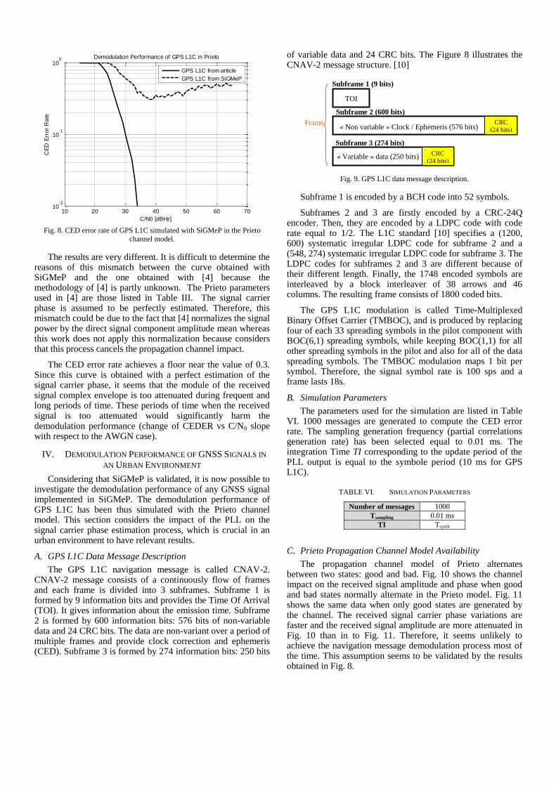
Fig. 8. CED error rate of GPS L1C simulated with SiGMeP in the Prieto
channel model.
The results are very different. It is difficult to determine the reasons of this mismatch between the curve obtained with SiGMeP and the one obtained with [4] because the methodology of [4] is partly unknown. The Prieto parameters used in [4] are those listed in Table III. The signal carrier phase is assumed to be perfectly estimated. Therefore, this mismatch could be due to the fact that [4] normalizes the signal power by the direct signal component amplitude mean whereas this work does not apply this normalization because considers that this process cancels the propagation channel impact.
The CED error rate achieves a floor near the value of 0.3. Since this curve is obtained with a perfect estimation of the signal carrier phase, it seems that the module of the received signal complex envelope is too attenuated during frequent and long periods of time. These periods of time when the received signal is too attenuated would significantly harm the demodulation performance (change of CEDER vs C/N0 slope with respect to the AWGN case).
IV. DEMODULATION PERFORMANCE OF GNSS SIGNALS IN
AN URBAN ENVIRONMENT
Considering that SiGMeP is validated, it is now possible to investigate the demodulation performance of any GNSS signal implemented in SiGMeP. The demodulation performance of GPS L1C has been thus simulated with the Prieto channel model. This section considers the impact of the PLL on the signal carrier phase estimation process, which is crucial in an urban environment to have relevant results.
A. GPS L1C Data Message Description
The GPS L1C navigation message is called CNAV-2. CNAV-2 message consists of a continuously flow of frames and each frame is divided into 3 subframes. Subframe 1 is formed by 9 information bits and provides the Time Of Arrival (TOI). It gives information about the emission time. Subframe 2 is formed by 600 information bits: 576 bits of non-variable data and 24 CRC bits. The data are non-variant over a period of multiple frames and provide clock correction and ephemeris (CED). Subframe 3 is formed by 274 information bits: 250 bits
of variable data and 24 CRC bits. The Figure 8 illustrates the CNAV-2 message structure. [10]
Fig. 9. GPS L1C data message description.
Subframe 1 is encoded by a BCH code into 52 symbols.
Subframes 2 and 3 are firstly encoded by a CRC-24Q encoder. Then, they are encoded by a LDPC code with code rate equal to 1/2. The L1C standard [10] specifies a (1200, 600) systematic irregular LDPC code for subframe 2 and a (548, 274) systematic irregular LDPC code for subframe 3. The LDPC codes for subframes 2 and 3 are different because of their different length. Finally, the 1748 encoded symbols are interleaved by a block interleaver of 38 arrows and 46 columns. The resulting frame consists of 1800 coded bits.
The GPS L1C modulation is called Time-Multiplexed Binary Offset Carrier (TMBOC), and is produced by replacing four of each 33 spreading symbols in the pilot component with BOC(6,1) spreading symbols, while keeping BOC(1,1) for all other spreading symbols in the pilot and also for all of the data spreading symbols. The TMBOC modulation maps 1 bit per symbol. Therefore, the signal symbol rate is 100 sps and a frame lasts 18s.
B. Simulation Parameters
The parameters used for the simulation are listed in Table VI. 1000 messages are generated to compute the CED error rate. The sampling generation frequency (partial correlations generation rate) has been selected equal to 0.01 ms. The integration Time TI corresponding to the update period of the PLL output is equal to the symbole period (10 ms for GPS L1C).
TABLE VI. SIMULATION PARAMETERS
Number of messages 1000
Tsampling 0.01 ms
TI Tsymb
C. Prieto Propagation Channel Model Availability
The propagation channel model of Prieto alternates between two states: good and bad. Fig. 10 shows the channel impact on the received signal amplitude and phase when good and bad states normally alternate in the Prieto model. Fig. 11 shows the same data when only good states are generated by the channel. The received signal carrier phase variations are faster and the received signal amplitude are more attenuated in Fig. 10 than in to Fig. 11. Therefore, it seems unlikely to achieve the navigation message demodulation process most of the time. This assumption seems to be validated by the results obtained in Fig. 8.
10 20 30 40 50 60 7010
-2
10-1
100 Demodulation Performance of GPS L1C in Prieto
C/N0 [dBHz]
CE
D E
rro
r R
ate
GPS L1C from article
GPS L1C from SiGMeP
TOI
Subframe 1 (9 bits)
« Non variable » Clock / Ephemeris (576 bits)
Subframe 2 (600 bits)
« Variable » data (250 bits)
Subframe 3 (274 bits)
CRC
(24 bits)
CRC
(24 bits)
Frame

Nevertheless, once the receiver has succeeded in demodulating at least once the CED and even if the message cannot be demodulated again, the receiver can determine its position for a while as long as it is able to compute pseudorange measurements (the ephemeris and the satellite clock correction terms are generally valid for a few hours). Therefore, successfully consecutive navigation message demodulations are not necessary for the receiver to provide its position. The GNSS signals demodulation performance in urban environment with SiGMeP is thus computed only with the channel model in good state configuration altogether with the channel availability for this specific reception conditions (see Table VII).
Fig. 10. Received signal amplitude and phase in the Prieto channel model case.
Fig. 11. Received signal amplitude and phase in the Prieto channel model
case, only with good states.
TABLE VII. AVAILABILITY OF THE PRIETO CHANNEL MODEL
CORRESPONDING TO GPS L1C
Frames for which the channel states are always good
3.4 %
Subframes 2 and 3 (CED interleaved with sub3) for which the channel states are always good
3.6 %
Symbols for which the channel states are always good
42.0 %
When the Prieto channel model is used with the parameters described in Table III with the GPS L1C signal (one navigation
message lasts 18 s and one symbol lasts 10 ms), 3.4% of the generated navigation messages and 42% of the generated symbols are entirely transmitted during a good state period. Concerning the CED (which correspond to the subframe 2 for GPS L1C), it is not possible to compute the availability only for the CED because the subframes 2 and 3 are interleaved. Therefore the percentage of generated subframes 2 and 3 entirely transmitted during a good state period is computed. It is equal to 3.6%.
D. Demodulation Performance
The demodulation performance of GPS L1C is computed using the SiGMeP software either with perfect signal carrier phase estimation or with PLL tracking, and with the Prieto propagation channel model but forcing the generation of good states only. The Loo parameters are drawn at each new message and remain unchanged during the entire message duration (corresponding to one same good state during one entire frame). In the perfect signal carrier phase estimation case, the estimated phase of each local replica sample phase is just equal to the corresponding propagation channel sample phase. Indeed, the received signal phase is assumed to be perfectly compensated. In the PLL case, the PLL uses as input the pilot channel of GPS L1C signal which does not carry data (it is just impacted by the propagation channel). The resulting phase estimated by the PLL is then used to correct the carrier phase introduced by the channel on the signal data component. The PLL parameters are listed in Table IV. Fig. 12 presents the CED error rate according to the signal to noise ratio, as well as the percentage of detected losses of lock in the PLL case (computed thanks to a Van Dierendonck detector), according to the signal to noise ratio.
Fig. 12. GPS L1C demodulation performance with the Prieto channel model
in good states configuration, with PLL tracking.
TABLE VIII. DETECTED LOSSES OF LOCK
𝑁
Percentage of detected losses
of lock in the PLL case 0 %
This curve represents the demodulation performance of GPS L1C in good states, i.e. in 3.4% of cases. From Fig 12, it can be observed that a CEDER of 10
-2 is obtained for a C/N0 of
26.1 dBHz, in the PLL tracking case. Moreover, it can be seen that 1 extra dB is required for a CEDER of 10
-2 with respect to
0 10 20 30 40 50 60 70 80 90
-60
-40
-20
0
20
Time (seconds)
Am
plitu
de
(d
B)
Received signal amplitude with the Prieto channel model (dB)
0 10 20 30 40 50 60 70 80 90-2
-1.5
-1
-0.5
0
0.5
1
1.5
2
Time (seconds)
Pha
se (
radia
ns)
Received signal phase with the Prieto channel model (radians)
0 10 20 30 40 50 60 70 80 90
-60
-40
-20
0
20
Time (seconds)
Am
plitu
de
(d
B)
Received signal amplitude with the Prieto channel model (dB)
0 10 20 30 40 50 60 70 80 90-2
-1.5
-1
-0.5
0
0.5
1
1.5
2
Time (seconds)
Pha
se (
radia
ns)
Received signal phase with the Prieto channel model (radians)
21 22 23 24 25 26 2710
-3
10-2
10-1
100
SiGMeP Demodulation Performance of GPS L1C in Prieto with only good states
C/N0 [dBHz]
CE
D E
rro
r R
ate
Perfect phase estimation-Prieto
PLL with ATAN2-Prieto
AWGN

an AWGN channel. Finally, the demodulation performance for an ideal signal carrier phase estimation is slight better than the demodulation performance when a PLL is implemented: about 0.5 dB for a CEDER of 10
-2. And it must be noticed that the
PLL tracking is never lost, according to the Van Dierendonck detector.
V. CONCLUSION AND FUTURE WORK
This paper has presented the SiGMeP simulation tool implementation, able to provide realistically GNSS signal demodulation performance in urban environments. Moreover, this paper provides the demodulation performance of GPS L1C signal using the Prieto channel model in good state configuration altogether with the availability of the channel. The Prieto channel model is forced to generate only good states in order to ensure that the demodulation process has a higher probability of success. The demodulation performance for a perfect signal carrier phase estimation has been computed. In addition, the paper shows the impact of the PLL on the signal carrier phase estimation process and thus on the demodulation process.
The SiGMeP simulation tool has only been partly validated; uncertainty about the Prieto channel model remains. Future work will address this issue. Moreover, the Prieto channel model is a narrowband model. Therefore, another further step will be to test a wideband channel model, which could better represent the reality.
REFERENCES
[1] Emmanuele, Andrea, Luise, Jong-Hoon Won, Diana Fontanella, Matteo Paonni, Bernd Eissfeller, Francesca Zanier, and Gustavo Lopez-Risueno.
2011. “Evaluation of Filtered Multitone FMT Technology for Future Satellite avigation Use.” In IO G SS 2011, Portland, OR.
[2] Emmanuele, A., F. Zanier, G. Boccolini, and M. uise. 2012. “Spread-Spectrum Continuous-Phase-Modulated Signals for Satellite avigation.” IEEE Transactions on Aerospace and Electronic Systems 48 (4).
[3] M. Anghileri, M. Paonni, D. Fontanella, and B. Eissfeller, “Assessing G SS Data Message Performance A ew Approach,” Inside GNSS, pp. 60–70, Apr. 2013.
[4] M. Anghileri, M. Paonni, D. Fontanella, and B. Eissfeller, “G SS Data Message Performance: A New Methodology for its Understanding and Ideas for its Improvement,” presented at the International Technical Meeting (ITM) of The Institute of Navigation, San Diego, CA, 2013.
[5] F. Pere -Fontan, M. A. ue -Castro, S. Buonomo, J. P. Poiares-Baptista, and B. Arbesser-Rastburg, “S-band LMS propagation channel behaviour for different environments, degrees of shadowing and elevation angles,” IEEE Trans. Broadcast., vol. 44, no. 1, pp. 40–76, 1998.
[6] F. P. Fontan, M. Vazquez-Castro, C. E. Cabado, J. P. Garcia, and E. Kubista, “Statistical modeling of the MS channel,” IEEE Trans. Veh. Technol., vol. 50, no. 6, pp. 1549–1567, 2001.
[7] R. Prieto-Cerdeira, F. Perez-Fontan, P. Burzigotti, A. Bolea-Alamañac, and I. Sanchez- ago, “ ersatile two-state land mobile satellite channel model with first application to DVB-SH analysis,” Int. J. Satell. Commun. Netw., vol. 28, no. 5–6, pp. 291–315, 2010.
[8] Parkinson, Bradford W., and James J. Spilker. 1996. Global Positioning System: Theory and Applications (volume One). AIAA.
[9] A. Garcia-Pena, “Optimi ation of Demodulation Performance of the GPS and GALILEO avigation Messages,” PhD, Université de Toulouse, 2010.
[10] US Government. 2012. “I TERFACE SPECIFICATIO IS-GPS-800 avstar GPS Space Segment/User Segment 1C Interface.”
[11] D. Tse, Fundamentals of Wireless Communication. Cambridge University Press, 2005.