GNU Numerical Electromagnetics Code(gNEC)

Theory

Version 0.9.15

2 February 2018

1

Preface

This manual builds on the work of many people, starting with the original authors who are ac-knowledged in the Preface to the Original NEC Program Description - Theory, reproduced inthe first subsection of this preface. The first edition of the manual was published in January 1981and was wholly paper based.

The manual was then scanned by Alexandre Kampouris and published as a PDF file in January1997. The preface to that edition is reproduced in the subsection Preface to the Scanned PDFEdition.

The manual was then transformed for the Web using OCR (Optical Character Recognition) byChuck Adams in June 2007. The preface to that edition of the manual is reproduced in the sub-section Preface to the Web Edition. Chuck produced a LaTeX version of the manual which wasconverted to a PDF file.

This current edition aimed at producing LaTeX source file/s which could be edited with a texteditor and be converted into any form (eg. PDF, PS or HTML) supported by LaTeX format con-version utilities. The initial step in generating this manual was to extract the text from ChuckAdams PDF file (with Chuck’s permission) using the utility pdftotext (part of the poppler pack-age under ArchLinux). The text was then converted to LaTeX by hand and the equations wheremanually entered as LaTeX instructions.

This edition of the manual isn’t intended simply as a copy of the original but an update, in supportof the gNEC project. Future plans include redrawing all figures using the LaTeX figure enviro-ment, and expanding explanations of the maths underpinning NEC, where appropriate.

Mike Waters

Preface to the Original NEC Program Description - Theory

The Numerical Electromagnetics Code (NEC) has been developed at the Lawrence LivermoreLaboratory, Livermore, California, under the sponsorship of the Naval Ocean Systems Centerand the Air Force Weapons Laboratory. It is an advanced version of the Antenna Modeling Pro-gram (AMP) developed in the early 1970’s by MBAssociates for the Naval Research Laboratory,Naval Ship Engineering Center, U.S. Army ECOM/Communications Systems, U.S. Army Strate-gic Communications Command, and Rome Air Development Center under Office of Naval Re-search Contract N00014-71-C-0187. The present version of NEC is the result of efforts by G. J.Burke and A. J. Poggio of Lawrence Livermore Laboratory.

The documentation for NEC consists of three volumes :

Part I : NEC Program Description - TheoryPart II : NEC Program Description - CodePart III : NEC User’s Guide

The documentation has been prepared by using the AMP documents as foundations and by modi-fying those as needed. In some cases this led to minor changes in the original documents while inmany cases major modifications were required.

2

Over the years many individuals have been contributors to AMP and NEC and are acknowledgedhere as follows :

• R. W. Adams • R. J. Lytle• J. N. Brittingham • E. K. Miller• G. J. Burke • J. B. Morton• F. J. Deadrick • G. M. Pjerrou• K. K. Hazard • A. J. Poggio• D. L. Knepp • E. S. Selden• D. L. Lager

The support for the development of NEC-2 at the Lawrence Livermore Laboratory has been pro-vided by the Naval Ocean Systems Center under MIPR-N0095376MP. Cognizant individuals un-der whom this project was carried out include : J. Rockway and J. Logan. Previous developmentof NEC also included the support of the Air Force Weapons Laboratory (Project Order 76-090)and was monitored by J. Castillo and TSgt. H. Goodwin.

Work was performed under the auspices of the U. S. Department of Energy by the LawrenceLivermore National Laboratory under contract No. W-7405-Eng-48. Reference to a company orproduct name does not imply approval or recommendation of the product by the University ofCalifornia or the U.S. Department of Energy to the exclusion of others that may be suitable.

Preface to the Scanned PDF Edition

This document (Part I) was scanned at a resolution of 196x204DPI and placed into a CCITT/G4encoded PDF. Only minor cosmetic changes were made to the file. The left handed and righthanded page data was recentered a bit. Some scanning noise, including punch holes, was elimi-nated. The scaling was chosen to (hopefully) make printing on DIN A4 paper possible. I make norepresentation whatsoever as to the usefulness or exactitude of this Acrobat file, nor can have anyresponsibility for that of the original document.

Have fun!

Alexandre Kampouris, MontrealE-Mail: ak@Radio-BIP.qc.ca

Preface to the Web Edition

This manual and the associated NEC-2 manuals are the result of a concerted effort to produce a setof clean documents for the NEC-2 program. The original manuals were first released in January1981 and are available from the US Government, but are of poor quality. Not the fault of anyindividual or group. It is just an illustration of the evolution of computer technology since the timeof using typewriters for the production of manuals and documentation. The original manuals arealso available online from several sources by doing a search for nec2part1.pdf, nec2part2.pdf, andnec2part3.pdf.

I have made an effort to correct as many errors as possible in the scanning of the documents and theOCR process itself. Any pointers to errors, either in the original documents or in my productionof these documents is greatly appreciated. I will make the appropriate corrections and reproducethe new document as soon as possible and place them back on the web.

These documents were produced using LaTeX under the kubuntu 7.04 Linux operating system ona Compaq Presario AMD 64 system. I have redone all the graphics where possible to improve the

3

quality of the documents. This work started in mid-June 2007 and most likely will continue for avery long time due to the immensity of the project.

I have chosen the fixed spacing typewriter font to reproduce the font used in the original docu-ments.

The program listing is slightly different from the original as shown in Part II of the original manual,so it will take a long time to match the program line numbers with the correct lines. Just pleasepatient as this work progresses.

Please note that all equations have been entered entirely by hand and are subject to extra scrutinyon the part of the reader.

Thanks.

Chuck Adams, K7QOPrescott, AZJune, 2007k7qo@commspeed.net

4

Disclaimer

This manual was originally prepared as an account of work sponsored by the United States Gov-ernment. Neither the United States nor the United States Department of Energy, nor any of theiremployees, nor any of their contractors, subcontractors, or their employees, makes any warranty,express or implied, or assumes any legal liability or responsibility for the accuracy, completenessor usefulness of any information, apparatus, product or process disclosed, or represents that its usewould not infringe privately-owned rights.

The Web (HTML) and Microsoft Word (WDBN) versions of this manual were derived from theoriginal, printed version by uncompensated volunteers, through optical scanning and automaticcharacter recognition (OCR), retyping, reformatting and other editing. These processes have in-evitably introduced errors and omissions, for which the United States Government, LawrenceLivermore National Laboratory and University of California have no responsibility. No assuranceis made by anyone as to the completeness, accuracy, or suitability for any purpose of any versionof this manual.

Users should be particularly alert for errors of the sort that occur frequently with OCR, eg. misseddecimal points and minus signs; confusion of the numeral "1", the lower-case letter "l", and theupper-case letter "I"; misalignment of columns in card images due to miscounting of spaces; andincorrect word substitution by automatic spell-checking programs.

This LaTeX version of the manual derives from a PDF copy of the Web version. Users should notethat, as yet only cursory checks of the accuracy of this manual have been made. The author can’tguarantee that there are no errors (and probably never will, as it’s provided at no cost). Havingsaid that, I endeavour to correct errors as they become known.

5

Contents

Title Page . . . . . . . . . . . . . . . . . . . . . . . . . . . . . . . . . . . . . . . . . 1Preface . . . . . . . . . . . . . . . . . . . . . . . . . . . . . . . . . . . . . . . . . . . 2Disclaimer . . . . . . . . . . . . . . . . . . . . . . . . . . . . . . . . . . . . . . . . . 5Table of Contents . . . . . . . . . . . . . . . . . . . . . . . . . . . . . . . . . . . . . 6List of Figures . . . . . . . . . . . . . . . . . . . . . . . . . . . . . . . . . . . . . . . 7

1 Introduction 8

2 The Integral Equations for Free Space 102.1 The Electric Field Integral Equation (EFIE) . . . . . . . . . . . . . . . . . . . . 112.2 The Magnetic Field Integral Equation (MFIE) . . . . . . . . . . . . . . . . . . . 132.3 The EFIE-MFIE Hybrid Equation . . . . . . . . . . . . . . . . . . . . . . . . . 14

3 Numerical Solution 153.1 Current Expansion on Wires . . . . . . . . . . . . . . . . . . . . . . . . . . . . 173.2 Current Expansion on Surfaces . . . . . . . . . . . . . . . . . . . . . . . . . . . 233.3 Evaluation of the Fields . . . . . . . . . . . . . . . . . . . . . . . . . . . . . . . 253.4 The Matrix Equation for Current . . . . . . . . . . . . . . . . . . . . . . . . . . 313.5 Solution of the Matrix Equation . . . . . . . . . . . . . . . . . . . . . . . . . . 32

4 Effect of Ground Plane 364.1 The Sommerfeld / Norton Method . . . . . . . . . . . . . . . . . . . . . . . . . 374.2 Numerical Evaluation of the Sommerfeld Integrals . . . . . . . . . . . . . . . . 464.3 The Image and Reflection-Coefficient Methods . . . . . . . . . . . . . . . . . . 50

5 Modelling of Antennas 545.1 Source Modeling . . . . . . . . . . . . . . . . . . . . . . . . . . . . . . . . . . 555.2 Nonradiating Networks . . . . . . . . . . . . . . . . . . . . . . . . . . . . . . . 605.3 Transmission Line Modeling . . . . . . . . . . . . . . . . . . . . . . . . . . . . 635.4 Lumped or Distributed Loading . . . . . . . . . . . . . . . . . . . . . . . . . . 655.5 Radiated Field Calculation . . . . . . . . . . . . . . . . . . . . . . . . . . . . . 675.6 Antenna Coupling . . . . . . . . . . . . . . . . . . . . . . . . . . . . . . . . . . 69

6

List of Figures

1 Current Basis Functions and Sum on a Four Segment Wire. . . . . . . . . . . . . 182 Segments Covered by the i-th Basis Function. . . . . . . . . . . . . . . . . . . . 183 Detail of the Connection of a Wire to a Surface. . . . . . . . . . . . . . . . . . . 244 Current-Filament Geometry for the Thin-Wire Kernel. . . . . . . . . . . . . . . 255 Current Geometry for the Extended Thin-Wire Kernel. . . . . . . . . . . . . . . 276 Coordinates for Evaluating the Field of a Current Element Over Ground. . . . . . 377 Real (a) and Imaginary (b) Parts of IV

ρ for ε1/εo = 4, σ1 = 0.001 mhos/m, fre-quency = 10 MHz. . . . . . . . . . . . . . . . . . . . . . . . . . . . . . . . . . 42

8 Real (a) and Imaginary (b) Parts of IVz for ε1/εo = 4, σ1 = 0.001 mhos/m, fre-

quency = 10 MHz. . . . . . . . . . . . . . . . . . . . . . . . . . . . . . . . . . 439 Real (a) and Imaginary (b) Parts of IH

ρ for ε1/εo = 4, σ1 = 0.001 mhos/m, fre-quency = 10 MHz. . . . . . . . . . . . . . . . . . . . . . . . . . . . . . . . . . 43

10 Real (a) and Imaginary (b) Parts of IHφ

for ε1/εo = 4, σ1 = 0.001 mhos/m, fre-quency = 10 MHz. . . . . . . . . . . . . . . . . . . . . . . . . . . . . . . . . . 44

11 Real (a) and Imaginary (b) Parts of IHρ for ε1/εo = 16, σ1 = 0.000 mhos/m, fre-

quency = 10 MHz. . . . . . . . . . . . . . . . . . . . . . . . . . . . . . . . . . 4412 Grid for Bivariate Interpolation of I’s. . . . . . . . . . . . . . . . . . . . . . . . 4513 Contour for Evaluation of Bessel Functions Form of Sommerfeld Integrals. . . . 4614 Contour for Evaluation of Hankel Functions Form of Sommerfeld Integrals. . . . 4815 Contour for Hankel Functions Form when Real Part k1 is Large and Imaginary

Part k1 is Small. . . . . . . . . . . . . . . . . . . . . . . . . . . . . . . . . . . . 4816 Plane-Wave Reflection at an Interface. . . . . . . . . . . . . . . . . . . . . . . . 5117 Biconical Transmission Line Model of Source Region. . . . . . . . . . . . . . . 5618 Field Plots for a Linear Dipole, Ω = 15. . . . . . . . . . . . . . . . . . . . . . . 5919 Voltage and Current Reference Directions at Network Ports. . . . . . . . . . . . 6120 Network Connection to Segments. . . . . . . . . . . . . . . . . . . . . . . . . . 6121 Network Port and Voltage Source Connected to a Segment. . . . . . . . . . . . . 6122 Current Distribution on a Two-Wire Transmission Line from NEC Compared with

the Ideal Transimission Line Solution. . . . . . . . . . . . . . . . . . . . . . . . 64

7

1 Introduction

The Numerical Electromagnetics Code (NEC) is a user-oriented computer code for the analysisof the electromagnetic response of antennas and other metal structures. It is built around thenumerical solution of integral equations for the currents induced on the structure by sources orincident fields. This approach avoids many of the simplifying assumptions required by othersolution methods and provides a highly accurate and versatile tool for electromagnetic analysis.

The code combines an integral equation for smooth surfaces with one specialized to wires toprovide for convenient and accurate modeling of a wide range of structures. A model may includenonradiating networks and transmission lines connecting parts of the structure, perfect or imperfectconductors, and lumped-element loading. A structure may also be modeled over a ground planethat may be either a perfect or imperfect conductor.

The excitation may be either voltage sources on the structure or an incident plane wave of linearor elliptic polarization. The output may include induced currents and charges, near electric ormagnetic fields, and radiated fields. Hence, the program is suited to either antenna analysis orscattering and EMP studies. NEC and its predecessor AMP have been used successfully to modela wide range of antennas including complex environments such as ships. Results from modelingseveral antennas with NEC are shown in refs. 36, 37, and 38 with measured data for comparison.

The integral-equation approach is best suited to structures with dimensions up to several wave-lengths. Although there is no theoretical size limit, the numerical solution requires a matrix equa-tion of increasing order as the structure size is increased relative to wavelength. Hence, modelingvery large structures may require more computer time and file storage than practical on a particularmachine. In such cases standard high-frequency approximations such as geometrical or physicaloptics, or geometric theory of diffraction may be more suitable than the integral equation approachused in NEC.

The code NEC-2 is the latest in a series of electromagnetics codes, each of which has built uponthe previous one. The first in the series was the code BRACT which was developed at MBAsso-ciates in San Ramon, California, under the funding of the Air Force Space and Missiles SystemsOrganization (refs. 1 and 2). BRACT was specialized to scattering by arbitrary thin-wire configu-rations.

The code AMP followed BRACT and was developed at MBAssociates with funding from theNaval Research Laboratory, Naval Ship Engineering Center, U.S. Army ECOM/CommunicationsSystems, U.S. Army Strategic Communications Command, and Rome Air Development Centerunder Office of Naval Research Contract N00014--71--C--0287. AMP uses the same numericalsolution method as BRACT with the addition of the capability of modeling a structure over aground plane and an option to use file storage to greatly increase the maximum structure size thatmay be modeled. The program input and output were extensively revised for AMP so that the codecould be used with a minimum of learning and computer programming experience. AMP includesextensive documentation to aid in understanding, using, and modifying the code (refs. 3, 4 and 5).

A modeling option specialized to surfaces was added to the wire modeling capabilities of AMPin the AMP2 code (ref. 6). A simplified approximation for large interaction distances was alsoincluded in AMP2 to reduce running time for large structures.

The code NEC-1 added to AMP2 a more accurate current expansion along wires and at multiplewire junctions, and an option in the wire modeling technique for greater accuracy on thick wires.A new model for a voltage source was added and several other modifications made for increasedaccuracy and efficiency.

8

NEC-2 retains all features of NEC-1 except for a restart option. Major additions in NEC-2 arethe Numerical Green’s Function for partitioned-matrix solution and a treatment for lossy groundsthat is accurate for antennas very close to the ground surface. NEC-2 also includes an option tocompute maximum coupling between antennas and new options for structure input.

Part I of this document describes the equations and numerical methods used in NEC. Part III: NECUser’s Guide (ref. 7) contains instructions for using the code, including preparation of input andinterpretation of output. Part II: NEC Program Description --- Code (ref. 8) describes the codingin detail. The user encountering the code for the first time should begin with the User’s Guideand try modeling some simple antennas. Part II will be of interest mainly to someone attemptingto modify the code. Reading part I will be useful to the new user of NEC-2, however, since anunderstanding of the theory and solution method will assist in the proper application of the code.

9

2 The Integral Equations for Free Space

The NEC program uses both an electric-field integral equation (EFIE) and a magnetic-field integralequation (MFIE) to model the electromagnetic response of general structures. Each equationhas advantages for particular structure types. The EFIE is well suited for thin-wire structures ofsmall or vanishing conductor volume while the MFIE, which fails for the thin-wire case, is moreattractive for voluminous structures, especially those having large smooth surfaces. The EFIE canalso be used to model surfaces and is preferred for thin structures where there is little separationbetween a front and back surface. Although the EFIE is specialized to thin wires in this program,it has been used to represent surfaces by wire grids with reasonable success for far-field quantitiesbut with variable accuracy for surface fields. For a structure containing both wires and surfacesthe EFIE and HFIE are coupled. This combination of the EFIE and MFIE was proposed and usedby Albertsen, Hansen, and Jensen at the Technical University of Denmark (ref. 9) although thedetails of their numerical solution differ from those in NEC. A rigorous derivation of the EFIE andMFIE used in NEC is given by Poggio and Hiller (ref. 10). The equations and their derivation areoutlined in the following sections.

10

2.1 The Electric Field Integral Equation (EFIE)

The form of the EFIE used in NEC follows from an integral representation for the electric field ofa volume current distribution ~J :

~E(~r ) =− jη4πk

∫V~J(~r ′) · G(~r,~r ′)dV ′ (1)

where

G(~r,~r ′) = (k2 I +∇∇)g(~r,~r ′)

g(~r,~r ′) =exp(− jk |~r−~r ′|)

|~r−~r ′|k = ω

√µoεo

η =√

µo/εo

and the time convention is exp( jωt). I is the identity dyad (xx + yy+ zz). When the currentdistribution is limited to the surface of a perfectly conducting body, Equation (1) becomes :

~E(~r ) =− jη4πk

∫S~Js(~r ′) · G(~r,~r ′)dA′ (2)

with ~Js the surface current density. The observation point~r is restricted to be off the surface S sothat~r 6=~r ′.

If~r approaches S as a limit, equation (2) becomes :

~E(~r ) =− jη4πk−∫

S~Js(~r ′) · G(~r,~r ′)dA′ (3)

where the principal value integral, −∫

, is indicated since g(~r,~r ′) is now unbounded.

An integral equation for the current induced on S by an incident field ~E I can be obtained fromequation (3) and the boundary condition for~r ε S :

n(~r )×[~ES(~r )+~E I(~r )

]= 0 (4)

where n(~r) is the unit normal vector of the surface at~r and ~ES is the field due to the induced current~JS. Substituting Equation (3) for ~ES yields the integral equation :

− n(~r)×~E I(~r) =− jη4πk

n(~r)×−∫

S~JS(~r ′) · (k2I +∇∇)g(~r,~r ′)dA′ (5)

The vector integral in equation (5) can be reduced to a scalar integral equation when the con-ducting surface S is that of a cylindrical thin wire, thereby making the solution much easier. Theassumptions applied for a thin wire, known as the thin-wire approximation, are as follows :

a. Transverse currents can be neglected relative to axial currents on the wire.b. The circumferential variation in the axial current can be neglected.c. The current can be represented by a filament on the wire axis.d. The boundary condition on the electric field need be enforced in the axial direction only.

11

These widely used approximations are valid as long as the wire radius is much less than thewavelength and much less than the wire length. An alternate kernel for the EFIE, based on anextended thin-wire approximation in which condition c is relaxed, is also included in NEC forwires having too large a radius for the thin-wire approximation.

From assumptions a, b and c, the surface current ~JS(~r) on a wire of radius a can be replaced by afilamentary current I where :

I(s)s = 2πa~JS(~r),s = distance parameter along the wire at~r ands = unit vector tangent to the wire axis at~r.

Equation (5) then becomes :

− n(~r)×~E I(~r) =− jη4πk

n(~r)×∫

LI(s′)(k2s′−∇

∂

∂ s′)g(~r,~r ′)ds′ (6)

where the integration is over the length of the wire. Enforcing the boundary condition in the axialdirection reduces Equation (6) to the scalar equation,

− s ·~E I(~r) =− jη4πk

∫L

I(s′)(k2s · s′− ∂ 2

∂ s∂ s′)g(~r,~r ′)ds′ (7)

Since~r ′ is now the point at s′ on the wire axis while~r is a point at s on the wire surface |~r−~r ′| ≥ aand the integrand is bounded.

12

2.2 The Magnetic Field Integral Equation (MFIE)

MFIE is derived from the integral representation for the magnetic field of a surface current distri-bution ~JS :

~Hs(~r ) =1

4π

∫S~JS(~r ′)×∇

′ g(~r,~r ′)dA′ (8)

where the differentiation is with respect to the integration variable~r ′ . If the current ~JS is inducedby an external incident field ~H ′ , then the total magnetic field inside the perfectly conductingsurface must be zero. Hence, for~r just inside the surface S :

~HI(~r)+ ~HS(~r) = 0 (9)

where ~HI is the incident field with the structure removed, and ~H S is the scattered field given byequation (8). The integral equation for ~JS may be obtained by letting~r approach the surface point~ro from inside the surface along the normal n(~ro) . The surface component of equation (9) withequation (8) substituted for ~HS is then :

−n(~ro)× ~HI(~ro) = n(~ro)×1

4πlim~r→~ro

∫S~JS(~r ′)×∇

′ g(~r,~r ′)dA′

where n(~ro) is the outward directed normal vector at~ro . The limit can be evaluated by using aresult of potential theory (ref. 12) to yield the integral equation :

− n(~ro)× ~HI(~ro) =−12~Js(~ro)+

14π−∫

Sn(~ro)×

[~JS(~r ′)×∇

′ g(~r,~r ′)]

dA′ (10)

For solution in NEC, this vector integral equation is resolved into two scalar equations along theorthogonal surface vectors t1 and t2 where :

t1(~ro)× t2(~ro) = n(~ro)

By using the identity ~u · (~v×~w) = (~u×~v) · ~w and noting that t1× n = −t2 and t2× n = t1 , thescalar equations can be written :

t2(~ro) · ~HI(~ro) =−12

t1(~ro) · ~Js(~ro)−1

4π−∫

St2(~ro) ·

[~Js(~r ′)×∇

′g(~ro,~r ′)]

dA′ (11)

−t1(~ro) · ~HI(~ro) =−12

t2(~ro) · ~Js(~ro)+1

4π−∫

St1(~ro) ·

[~Js(~r ′)×∇

′g(~ro,~r ′)]

dA′ (12)

These two components suffice since there is no normal component of equation (10).

13

2.3 The EFIE-MFIE Hybrid Equation

Program NEC uses the EFIE for thin wires and the MFIE for surfaces. For a structure consistingof both wires and surfaces, vecr in equation (7) is restricted to the wires, with the integral forES(~r ), extending over the complete structure. The thin-wire form of the integral in equation (7) isused over wires while the more general form of equation (5) must be used on surfaces. Likewise,~ro is restricted to surfaces in equations (11) and (12), with the integrals for HS(~r ) extending overthe complete structure. On wires the integral is simplified by the thin-wire approximation. Theresulting coupled integral equations are, for~r on wire surfaces :

− s ·~E I(~r) =− jη4πk

∫L

I(s′)(

k2s · s′− ∂ 2

∂ s∂ s′

)g(~r,~r ′)ds′

− jη4πk

∫S1

~Js(~r) ·[

k2s′−∇′ ∂

∂ s

]g(~r,~r ′)dA′ (13)

and for~r on surfaces excluding wires :

t2(~r) · ~HI(~r) =− 14π

t2(~r) ·∫

LI(s′)

(s′×∇

′g(~r,~r ′))

ds′− 12

t1(~r) · ~Js(~ro) −

14π−∫

S1

t2(~r) ·[~Js(~r ′)×∇

′g(~ro,~r ′)]

dA′ (14)

and

− t1(~r) · ~HI(~r) =1

4πt1(~r) ·

∫L

I(s′)(s′×∇

′g(~r,~r ′))

ds′− 12

t2(~r) · ~Js(~ro) +

14π−∫

S1

t1(~r) ·[~Js(~r ′)×∇

′g(~ro,~r ′)]

dA′ (15)

The symbol L represents integration over wires while∫

S1represents integration over surfaces ex-

cluding wires. The numerical method used to solve equations (13), (14) and (15) is described insection III.

14

3 Numerical Solution

The integral equations (l3), (l4), and (l5) are solved numerically in NEC by a form of the method ofmoments. An excellent general introduction to the method of moments can be found in a book byR. F. Harrington, Field Computation by Moment Methods (ref. 13). A brief outline of the methodfollows.

The method of moments applies to a general linear-operator equation :

L f = e (16)

where f is an unknown response, e is a known excitation, and L is a linear operator (an integral op-erator in the present case). The unknown function f may be expanded in a sum of basis functions,f j , as :

f =N

∑j=1

α j f j (17)

A set of equations for the coefficients α j are then obtained by taking the inner product or equation(16) with a set of weighting functions |wi| ,

< wi,L f >=< wi,e > i = 1,2, ....N (18)

Due to the linearity of L equation (17) substituted for f yields :

N

∑j−1

α j < wi,L f >=< wi,e > i = 1,2, ....N (19)

This equation can be written in matrix notation as :

[G][A] = [E]

where

Gi j = < wi,L f >A j = α j

Ei = < wi,e >

The solution is then :[A] = [G]−1[E]

For the solution of equations (13), (l4), and (l5), the inner product is defined as :

< f ,g >=∫

Sf (~r)g(~r)dA

where the integration is over the structure surface. Various choices are possible for the weightingfunction wi and basis functions f j. When wi = fi , the procedure is known as Galerkin’smethod. In NEC the basis functions are different, wi being chosen as a set of delta functions :

wi(~r) = δ (~r−~ri)

with ~ri a set of points on the conducting surface. The result is a point sampling of the integralequations known as the collocation method of solution. Wires are divided into short straight

15

segments with a sample point at the center of each segment while surfaces are approximated by aset of flat patches or facets with a sample point at the center of each patch.

The choice of basis functions is very important for an efficient and accurate solution. In NEC thesupport of fi is restricted to a localized subsection of the surface near~ri . This choice simplifiesthe evaluation of the inner-product integral and ensures that the matrix G will be well conditioned.For finite N , the sum of f j cannot exactly equal a general current distribution, so the functions fi

should be chosen as close as possible to the actual current distribution. Because of the nature ofthe integral-equation kernels, the choice of basis function is much more critical on wires than onsurfaces. The functions used in NEC are explained in the following sections.

16

3.1 Current Expansion on Wires

Wires in NEC are modeled by short straight segments with the current on each segment representedby three terms - a constant, a sine, and a cosine. This expansion was first used by Yeh and Mei(ref. 14) and has been shown to provide rapid solution convergence (ref. 15 and 16). It hasthe added advantage that the fields of the sinusoidal currents are easily evaluated in closed form.The amplitudes of the constant, sine and cosine terms are related such that their sum satisfiesphysical conditions on the local behavior of current and charge at the segment ends. This differsfrom AMP where the current was extrapolated to the centers of the adjacent segments, resulting indiscontinuities in current and charge at the segment ends. Matching at the segment ends improvesthe solution accuracy, especially at the multiple-wire junctions of unequal length segments whereAMP extrapolated to an average length segment, often with inaccurate results.

The total current on segment number j in NEC has the form :

I j(s) = A j +B j sin(k(s− s j))+C j cos(k(s− s j)) (20)

|s− s j|<∆ j

2

where s j is the value of s at the center of segment i and ∆ j is the length of segment j. Of the threeunknown constants A j , B j , and C j , two are eliminated by local conditions on the current leavingone constant, related to the current amplitude, to be determined by the matrix equation. The localconditions are applied to the current and to the linear charge density, q, which is related to thecurrent by the equation of continuity :

δ Iδ s

=− jwq (21)

At a junction of two segments with uniform radius, the obvious conditions are that the current andcharge are continuous at the junction. At a junction of two or more segments with unequal radii,the continuity or current is generalized to Kirchoff’s current law that the sum of currents into thejunction is zero. The total charge in the vicinity of the junction is assumed to distribute itself onindividual wires according to the wire radii, neglecting local coupling effects. T. T. Wu and R. W.P. King (ref. l7) have derived a condition that the linear charge density on a wire at a junction, andhence δ I/δ s, is determined by :

δ I(s)δ s

∣∣∣∣s at junction

=Q

ln( 2

ka

)− γ

(22)

where

a = wire radiusk = 2π/λ

γ = 0.5772 (Euler’s constant)

Q is related to the total charge in the vicinity of the junction and is constant for all wires at thejunction.

At a free wire end, the current may be assumed to go to zero. On a wire of finite radius, however,the current can flow onto the end cap and hence be nonzero at the wire end. In one study of thiseffect, a condition relating the current at the wire end to the current derivative was derived (ref.18). For a wire or radius a , this condition is :

I(s)∣∣∣∣s at end

=−(s · nc)

kJ1(ka)J0(ka)

δ I(s)δ s

∣∣∣∣s at end

17

Figure 1: Current Basis Functions and Sum on a Four Segment Wire.

Figure 2: Segments Covered by the i-th Basis Function.

where J0 and J1 are Bessel functions of order 0 and 1. The unit vector nc is normal to the end cap.Hence, s · nc is +1 if the reference direction, s , is toward the end, and -1 if s is away from the end.

Thus, for each segment two equations are obtained from the two ends :

I j(s j±∆ j/2) =±1k

J1(ka j)

J0(ka j)

δ I j(s)δ s

∣∣∣∣s=s j±∆ j/2

(23)

at the free ends, and :δ I j(s)

δ s

∣∣∣∣s=s j±∆ j/2

=Q±j

ln(

2ka j

)− γ

(24)

at junctions. Two additional unknowns Q−j and Q+j are associated with the junctions but can be

eliminated by Kirchoff’s current equation at each junction. The boundary-condition equations pro-vide the additional equation-per-segment to completely determine the current function of equation(20) for every segment.

To apply these conditions, the current is expanded in a sum of basis functions chosen so that theysatisfy the local conditions on current and charge in any linear combination. A typical set of basisfunctions and their sum on a four segment wire are shown in Figure 1. For a general segment i inFigure 2, the i-th basis function has a peak on segment i and extends onto every segment connectedto i, going to zero with zero derivative at the outer ends of the connected segments.

18

The general definition of the i-th basis function is given below. For the junction and end conditionsdescribed above, the following definitions apply for the factors in the segment end conditions :

a−i = a+i =

[ln(

2kai

)− γ

]−1

(25)

and

Xi =J1(kai

J0(kai

The condition of zero current at a free end may be obtained by setting Xi to zero.

The portion of the i-th basis function on segment i is then :

f oi (s) = Ao

i +Boi sin(k(s− si))+Co

i cos(k(s− si)) (26)

|s− si|<∆i

2If N− 6= 0 and N+ 6= 0 , end conditions are :

δ f oi (s)δ s

∣∣∣∣s=si−∆i/2

= a−i Q−i (27)

δ f oi (s)δ s

∣∣∣∣s=si+∆i/2

= a+i Q+i (28)

If N− = 0 and N+ 6= 0 , end conditions are :

f oi (si−∆i/2) =

1k

Xiδ f o

i (s)δ s

∣∣∣∣s=si−∆i/2

(29)

δ f oi (s)δ s

∣∣∣∣s=si+∆i/2

= a+i Q+i (30)

If N− 6= 0 and N+ = 0 , end conditions are :

δ f oi (s)δ s

∣∣∣∣s=si−∆i/2

= a−i Q−i (31)

f oi (si +∆i/2) =

−1k

Xiδ f o

i (s)δ s

∣∣∣∣s=si+∆i/2

(32)

Over segments connected to end 1 of segment i , the i-th basis function is :

f−j (s) = A−j +B−j sin(k(s− s j))+C−j cos(k(s− s j)) (33)

|s− s j|<∆ j

2j = 1, .... ,N−

End conditions are :

f−j (s j−∆ j/2) = 0 (34)

δ f−j (s)

δ s

∣∣∣∣s=s j−∆ j/2

= 0 (35)

δ f−j (s)

δ s

∣∣∣∣s=si+∆i/2

= a+j Q−i (36)

19

Over segments connected to end 2 of segment i , the i-th basis function is :

f+j (s) = A+j +B+

j sin(k(s− s j))+C+j cos(k(s− s j)) (37)

|s− s j|<∆ j

2j = 1, .... ,N+

End conditions are :

δ f+j (s)

δ s

∣∣∣∣s=si−∆i/2

= a−j Q+i (38)

f+j (s j +∆ j/2) = 0 (39)

δ f+j (s)

δ s

∣∣∣∣s=s j+∆ j/2

= 0 (40)

Equations (26), (33) and (37), defining the complete basis function, involve 3(N−+N++ 1) un-known constants. Of these, 3(N−+N+)+ 2 unknowns are eliminated by the end conditions interms of Q−i and Q+

i which can then be determined from the two Kirchoff current equations :

N−

∑j=1

f−j (s j +∆ j/2) = f oi (si−∆i/2) (41)

N+

∑j=1

f+j (s j−∆ j/2) = f oi (si +∆i/2) (42)

The complete basis function is then defined in terms of one unknown constant. In this case A0i was

set to −1 since the function amplitude is arbitrary, being determined by the boundary conditionequations. The final result is given below :

A−j =a+j Q−i

sin(k∆ j)(43)

B−j =a+j Q−i

2cos(k∆ j/2)(44)

C−j =−a+j Q−i

2sin(k∆ j/2)(45)

A+j =−a−j Q+

i

sin(k∆ j)(46)

B+j =

a−j Q+i

2cos(k∆ j/2)(47)

C+j =

a−j Q+i

2sin(k∆ j/2)(48)

(49)

20

For N− 6= 0 and N+ 6= 0 :

Aoi =−1 (50)

Boi =

(a−i Q−i +a+i Q+

i

) sin(k∆i/2)sin(k∆i)

(51)

Coi =

(a−i Q−i −a+i Q+

i

) cos(k∆i/2)sin(k∆i)

(52)

Q−i =a+i (1− cos(k∆i))−P+

1 sin(k∆i)(P−i P+

i +a−i a+i)

sin(k∆i)+(P−i a+i −P+

i a−i)

cos(k∆i)(53)

Q+i =

a−i (cos(k∆i)−1)−P−1 sin(k∆i)(P−i P+

i +a−i a+i)

sin(k∆i)+(P−i a+i −P+

i a−i)

cos(k∆i)(54)

For N− = 0 and N+ 6= 0 :

Aoi =−1 (55)

Boi =

sin(k∆i/2)cos(k∆i)−Xi sin(k∆i)

+a+i Q+i

(cos(k∆i/2)−Xi sin(k∆i/2)

cos(k∆i)−Xi sin(k∆i)

)(56)

Coi =

cos(k∆i/2)cos(k∆i)−Xi sin(k∆i)

+a+i Q+i

(sin(k∆i/2)+Xi cos(k∆i/2)

cos(k∆i)−Xi sin(k∆i)

)(57)

Q+i =

cos(k∆i)−1−Xi sin(k∆i)(a+i +XiP+

i

)sin(k∆i)+

(a+i Xi−P+

i

)cos(k∆i)

(58)

For N− 6= 0 and N+ = 0 :

Aoi =−1 (59)

Boi =

−sin(k∆i/2)cos(k∆i)−Xi sin(k∆i)

+a−i Q−i

(cos(k∆i/2)−Xi sin(k∆i/2)

cos(k∆i)−Xi sin(k∆i)

)(60)

Coi =

cos(k∆i/2)cos(k∆i)−Xi sin(k∆i)

−a−i Q−i

(sin(k∆i/2)+Xi cos(k∆i/2)

cos(k∆i)−Xi sin(k∆i)

)(61)

Q−i =1− cos(k∆i)+Xi sin(k∆i)(

a−i −XiP−i)

sin(k∆i)+(P−i +Xia−i

)cos(k∆i)

(62)

For all cases :

P−i =N−

∑j=1

(1− cos(k∆i)

sin(k∆i)

)a+j (63)

P+i =

N+

∑j=1

(cos(k∆i)−1

sin(k∆i)

)a−j (64)

where the sum for P−i is over segments connected to end 1 of segment i, and the sum for P+i is

over segments connected to end 2. If N− = N+ = 0 , the complete basis function is :

f 0i =

cos(k(s− si))

cos(k∆i/2)−Xi sin(k∆i/2)−1 (65)

When a segment end is connected to a ground plane or to a surface modeled with the MFIE, theend condition on both the total current and the last basis function is :

δ I j(s)δ s

∣∣∣∣s=s j±∆ j/2

= 0

21

replacing the zero current condition at a free end. This condition does not require a separatetreatment, however, but is obtained by computing the last basis function as if the last segment isconnected to its image segment on the other side of the surface.

It should be noted that in AMP, the basis function fi has unit value at the center of segment iand zero value at the centers of connected segments although it does extend onto the connectedsegments. As a result, the amplitude of fi is the total current at the center of segment i . Thisis not true in NEC so the current at the center of segment i must be computed by summing thecontributions of all basis functions extending onto segment i.

22

3.2 Current Expansion on Surfaces

Surfaces on which the MFIE is used are modeled by small flat patches. The surface current oneach patch is expanded in a set of pulse functions except in the region of wire connection, as willbe described later. The pulse function expansion for Np patches is :

~JS(~r ) =Np

∑j=1

(J1 jt1 j + J2 jt2 j)Vj(~r ) (66)

where

t1 j = t1(~r j)

t2 j = t2(~r j)

~r j = position of the center of patch number j

Vj(~r ) = 1 for~r on patch j and 0 otherwise

The constants J1 j and J2 j , representing average surface-current density over the patch, are deter-mined by the solution of the linear system of equations derived from the integral equations. Theintegrals for fields due to the pulse basis functions, are evaluated numerically in a single step sothat for integration, the pulses could be reduced to delta functions at the patch centers. That thissimple approximation of the current yields good accuracy is one of the advantages of the MFIEfor surfaces.

A more realistic representation of the surface current is needed however, in the region where a wireconnects to the surface. The treatment used in NEC, affecting the four coplanar patches about theconnection point is quite similar to that used by Albertsen et al. (ref. 9). In the region of the wireconnection, the surface current contains a singular component due to the current flowing from thewire onto the surface. The total surface current should satisfy the condition :

∆s · ~Js(x,y) = Jo(x,y)+ Io δ (x,y)

where the local coordinates x and y are defined in figure 3, ∆s denotes surface divergence, Jo(x,y)is a continuous function in the region ABCD, and Io is the current at the base of the wire flowingonto the surface. One expansion which meets this requirement is :

~Js(x,y) = Io ~f (x,y)+4

∑j=1

g j(x,y)(~J j− Io ~f j

)(67)

where

~f (x,y) =xx+ yy

2π (x2 + y2)

~J j = ~Js(x j,y j)

~f j = ~f (x j,y j)

(x j,y j) = (x,y) at the center of patch j

The interpolation functions g j(x,y) are chosen such that :

• g j(x,y) is differentiable on ABCD,• g j(xi,yi) = δi j and• ∑

4j=1 g j(x,y) = 1.

23

Figure 3: Detail of the Connection of a Wire to a Surface.

The specific functions used in NEC are as follows :

g1(x,y) =1

4d2 (d + x)(d + y)

g2(x,y) =1

4d2 (d− x)(d + y)

g3(x,y) =1

4d2 (d− x)(d− y)

g4(x,y) =1

4d2 (d + x)(d− y)

Equation (66) is used when computing the electric field at the center of the connected wire segmentdue to the surface current on the four surrounding patches. In computing the field on any othersegments or on any patches, the pulse-function form is used for all patches including those at theconnection point. This saves integration time and is sufficiently accurate for the greatest source toobservation-point separations involved.

24

Figure 4: Current-Filament Geometry for the Thin-Wire Kernel.

3.3 Evaluation of the Fields

The current on each wire segment has the form :

Ii(s) = Ai +Bi sin(k(s− si))+Ci cos(k(s− si)) (68)

where

|s− si|<∆ j

2k =√

µoεo

∆i = the segment length

The solution requires the evaluation of the electric field at each segment due to this current. Threeapproximations or the integral equation kernel are used - a thin-wire form for most cases, anextended thin-wire form for thick wires, and a current element approximation for large interactiondistances. In each case the evaluation of the field is greatly simplified by the use of formulas forthe fields of the constant and sinusoidal current components.

The accuracy of the thin-wire approximation for a wire of radius a and length |Delta depends on kaand ∆/a . Studies have shown that the thin-wire approximation leads to errors of less than 1%, for∆/a greater than 8 (ref. 11). Furthermore, in the numerical solution of the EFIE, the wire is dividedinto segments less than about 0.1 λ in length to obtain an adequate representation of currentdistribution thus restricting ka to less than about 0.08. The extended thin-wire approximation isapplicable to shorter and thicker segments, resulting in errors less than 1%, for ∆/a greater than 2.

For the thin-wire kernel, the source current is approximated by a filament on the segment axiswhile the observation point is on the surface of the observation segment. The fields are evaluatedwith the source segment on the axis of a local cylindrical-coordinate system as illustrated in Figure4.

25

Then with :

Go =exp(− jkro)

ro(69)

ro =√

ρ2 +(z− z′)2 (70)

the ρ and z components of the electric field at P due to a sinusoidal current filament of arbitraryphase :

I = sin(kz′−Θo) , z1 < z′ < z2 (71)

are :

E fρ (ρ,z) =

− jη2k2λρ

[(z′− z) I

δGo

δ z′+ I Go− (z′− z)Go

δ Iδ z′

]z2

z1

(72)

E fz (ρ,z) =

jη2k2λ

[Go

δ Iδ z′− I

δGo

δ z′

]z2

z1

(73)

For a current that is constant over the length of the segment with strength I, the fields are :

E fρ (ρ,z) =

Iλ

jη2k2

[δGo

δρ

]z2

z1

(74)

E fρ (ρ,z) =−

Iλ

jη2k2

[δGo

δ z′

]z2

z1

+ k2∫ z2

z1

Go dz′

(75)

These field expressions are exact for the specified currents. The integral over z′ of Go is evaluatednumerically in NEC.

Substituting sine and cosine currents and evaluating the derivatives yields the following equationsfor the fields. For :

I = Io

(sin(kz′)cos(kz′)

)(76)

E fρ (ρ,z) =

−Io

λ

jη2k2ρ

Go

k(z− z′)

(cos(kz′)−sin(kz′)

)+

[1− (z− z′)2(1+ jkro)

1r2

o

](sin(kz′)cos(kz′)

)∣∣∣∣z2

z1

(77)

E fz (ρ,z) =

Io

λ

jη2k2 Go

k(

cos(kz′)−sin(kz′)

)− (z− z′)(1+ jkro)

1r2

o

(sin(kz′)cos(kz′)

)∣∣∣∣z2

z1

(78)

For a constant current of strength Io :

E fρ (ρ,z) =−

Io

λ

jηρ

2k2

[(1+ jkro)

Go

r2o

]z2

z1

(79)

E fz (ρ,z) =−

Io

λ

jη2k2

[(1+ jkro)(z− z′)

Go

r2o

]z2

z1

+ k2∫ z2

z1

Go dz′

(80)

Despite the seemingly crude approximation, the thin-wire kernel does accurately represent theeffect of wire radius for wires that are sufficiently thin. The accuracy range was studied by Poggioand Adams (ref. 11) where an extended thin-wire kernel was developed for wires that are too thickfor the thin-wire approximation.

The derivation of the extended thin-wire kernel starts with the current on the surface of the sourcesegment with surface density :

J(z′) =I(z′)2πa

26

Figure 5: Current Geometry for the Extended Thin-Wire Kernel.

where a is the radius of the source segment. The geometry for evaluation of the fields is shown infigure 5. A current filament of strength Idφ/(2π) is integrated over φ with :

ρ′ =√

ρ2 +a2−2aρ cosφ (81)

r =√

ρ ′ 2 +(z− z′)2 (82)

Thus, the z component of the field of the current tube is :

Etz(ρ,z) =

12π

∫ 2π

0E f

z (ρ′,z) dφ (83)

For the ρ component of field, the change in the direction of ρ ′ must be considered. The field inthe direction ρ is :

Etρ(ρ,z) =

12π

∫ 2π

0E f

ρ (ρ′,z)(ρ · ρ ′) dφ (84)

where

ρ · ρ ′ = ρ−acosφ

ρ ′=

δρ ′

δρ

The integrals over φ in equations (82) and (83) cannot be evaluated in closed form. Roggio andAdams, however, have evaluated them as a series in powers of a2 (ref. 11). The first term in theseries gives the thin-wire kernel. For the extended thin-wire kernel, the second term involving a2

is retained with terms of order a4 neglected. As with the thin-wire kernel, the field observationpoint is on the segment surface. Hence, when evaluating the field on the source segment, ρ = a.

The field equations with the extended thin-wire approximation are given below. For a sinusoidalcurrent of equation (70) :

Eρ(ρ,z) =− jη2k2λ

[(z′− z) I

δG2

δ z′+ I G2− (z′− z)G2

δ Iδ z′

]z2

z1

(85)

Ez(ρ,z) =jη

2k2λ

[G1

δ Iδ z′− I

δG1

δ z′

]z2

z1

(86)

27

For a constant current of strength Io :

Eρ(ρ,z) =Iλ

jη2k2

[δG1

δρ

]z2

z1

(87)

Ez(ρ,z) =−Iλ

jη2k2

[δG1

δ z′

]z2

z1

+ k2[

1− (ka)2

4

]∫ z2

z1

Go dz′− (ka)2

4

[δGo

δ z′

]z2

z1

(88)

The term G1 is the series approximation of :

Gt1 =

12π

∫ 2π

0Gdφ (89)

where

G =exp(− jkr)

rNeglecting terms of order a4 :

G1 = G0

1− a2

2r2o(1+ jkro)+

a2ρ2

4r4o

[3(1+ jkro)− k2r2

o]

(90)

δG1

δ z′=

(z− z′)r2

oG0

(1+ jkro)−

a2

2r2o

[3(1+ jkro)− k2r2

o]− a2ρ2

4r4o

[jk3r3

o +6k2r2o−15(1+ jkro)

](91)

δG1

δρ=

ρGo

r2o

(1+ jkro)−

a2

r2o

[3(1+ jkro)− k2r2

o]− a2ρ2

4r4o

[jk3r3

o +6k2r2o−15(1+ jkro)

](92)

The term G2 is the series approximation of :

Gt2 =

12π

∫ 2π

0

ρ−acosφ

ρ ′ 2Gdφ (93)

To order a2 :

G2 =G0

ρ

1+

a2ρ2

4r4o

[3(1+ jkro)− k2r2

o]

(94)

δG2

δ z′=

(z− z′)ρr2

oG0

(1+ jkro)−

a2ρ2

4r4o

[jk3r3

o +6k2r2o−15(1+ jkro)

](95)

Equation (86) makes use of the relation :

(ρ, ρ ′)δGδρ ′

=δGδρ ′

δρ ′

δρ ′=

δGδρ

(96)

while equation (87) follows from :

G1 =

[1− (ka)2

4− a2

4δ 2

δ z′2

]G0 (97)

When the observation point is within the wire (ρ < a) , a series expansion in ρ rather than a isused for G0 and G2 . For G1 this simply involves interchanging ρ and a in equations (89) and (90).Then for ρ < a , with :

ra =√

a2 +(z− z′)2 (98)

Ga =exp(− jkra)

ra(99)

28

the expressions for G1, G2 and their derivatives are :

G1 = Ga

1− ρ2

2r2a(1+ jkra)+

a2ρ2

4r4a

[3(1+ jkra)− k2r2

a]

(100)

δG1

δ z′=

(z− z′)r2

aGa

(1+ jkra)−

ρ2

2r2a

[3(1+ jkra)− k2r2

a]− a2ρ2

4r4a

[jk3r3

a +6k2r2a−15(1+ jkra)

](101)

δG1

δρ=− ρ

r2a

Ga

(1+ jkra)−

a2

2r2a

[3(1+ jkra)− k2r2

a]

(102)

G2 =−ρ

2r2a

Ga(1+ jkra) (103)

δG2

δ z′=−(z− z′)ρ

2r4a

Ga[3(1+ jkra)− k2r2

a]

(104)

Special treatment of bends in wires is required when the extended thin wire kernel is used. Theproblem stems from the cancellation of terms evaluated at z1 and z2 in the field equations whensegments are part of a continuous wire. The current expansion in NEC results in a current having acontinuous value and derivative along a wire without junctions. This ensures that for two adjacentsegments on a straight wire, the contributions to the z component of electric field at z2 , of thefirst segment exactly cancel the contributions from z1 representing the same point, for the secondsegment. For a straight wire or several segments, the only contributions for Ez with either thethin-wire or extended thin-wire kernel come from the two wire ends and the integral of G0 alongthe wire. For the ρ component of field or either component at a bend, while there is not completecancellation, there may be partial cancellation of large end contributions.

The cancellation of end terms makes necessary a consistent treatment of the current on both sidesof a bend for accurate evaluation of the field. This is easily accomplished with the thin-wire kernelsince the current filament on the wire axis is physically continuous around a bend. However, thecurrent tube assumed for the extended thin-wire kernel cannot be continuous around its completecircumference at a bend. This was found to reduce the solution accuracy when the extended thin-wire kernel was used for bent wires.

To avoid this problem in NEC, the thin-wire form of the end terms in equation (71) through (74) isalways used at a bend or change in radius. The extended thin-wire kernel is used only at segmentends where two parallel segments join, or at free ends. The switch from extended thin-wire tothe thin-wire form is made from one end of a segment to the other rather than between segmentswhere the cancellation of terms is critical.

When segments are separated by a large distance, the interaction may be computed with sufficientaccuracy by treating the segment current as an infinitesimal current element at the segment center.In spherical coordinates with the segment at the origin along the θ = 0 axis, the electric field is :

Er(r,θ) =Mη

2πr2 exp(− jkr)(

1− jkr

)cosθ

Eθ (r,θ) =Mη

4πr2 exp(− jkr)(

1+ jkr− jkr

)sinθ

The dipole moment M for a constant current I on a segment of length ∆i is :

M = I ∆i

29

For a current I cos[k(s− si)] with |s− si|< ∆/2 :

M =2Ik

sin(

k∆i

2

)while for a current I sin[k(s− si)] :

M = 0

Use of this approximation saves a significant amount of time in evaluating the interaction matrixelements for large structures. The minimum interaction distance at which it is used is selected bythe user in NEC. A default distance of one wavelength is set, however.

For each of the three methods of computing the field at a segment due to the current on anothersegment, the field is evaluated on the surface of the observation segment. Rather than choosing afixed point on the segment surface, the field is evaluated at the cylindrical coordinates (ρ ′,z withthe source segment at the origin. If the center point on the axis of the observation segment is at(ρ,z) , then :

ρ′ =√

ρ2 +a20

where a0 is the radius of the observation segment. Also, the component of Eρ tangent to theobservation segment is computed as :

~Eρ · s = (ρ · s) ρ

ρ ′Eρ

Inclusion of the factor ρ/ρ ′ , which is the cosine of the angle between ρ and ρ ′ , is necessary foraccurate results at bends in thick wires.

30

3.4 The Matrix Equation for Current

For a structure having Ns wire segments and Np patches, the order of the matrix in equation (l9)is N = Ns + 2Nρ . In NEC the wire segment equations occur first in the linear system so that, interms of submatrices, the equation has the form :A B

C D

Iw

Ip

=

Ew

Hp

with equations derived from equation (14) in odd numbered rows in the lower set and equation(15) in even rows. Iw is then the column vector of segment basis function amplitudes, and Ip isthe patch-current amplitudes (J1 j,J2 j, j = 1, ...,Np) The elements of Ew are the left-hand side ofequation (13) evaluated at segment centers, while Hp contains, alternately, the left-hand sides ofequations (14) and (15) evaluated at patch centers.

A matrix element Ai j , in submatrix A, represents the electric field at the center of segment i dueto the j-th segment basis function, centered on segment j. A matrix element Di j in submatrixD represents a tangential magnetic fie1d component at patch k due to a surface-current pulse onpatch l where :

k = Int[(i−1)/2]+1

l = Int[( j−1)/2]+1

and Int[ ] indicates truncation. The source pulse is in the direction t1 when j is odd, and directiont2 when j is even. When k = l the contribution of the surface integral is zero since the vectorproduct is zero on the flat patch surface, although a ground image may produce a contribution.However, for k = l, there is a contribution of ±1/2 from the coefficient of ~Js(~r ) in equation (14)or (15). Matrix elements in submatrices B and C represent electric fields due to surface-currentpulses and magnetic fields due to segment basis functions, respectively. These present no specialproblems since the source and observation points are always separated.

31

3.5 Solution of the Matrix Equation

The matrix equation :[G] [I] = [E] (105)

is solved in NEC by Gauss elimination (ref. 19). The basic step is factorization of the matrix Ginto the product of an upper triangular matrix U and a lower triangle matrix L where :

[G] = [L] [U ]

The matrix equation is then :[L] [U ] [I] = [E] (106)

from which the solution, I , is computed in two steps as :

[L] [F ] = [E] (107)

and :[U ] [I] = [F ] (108)

Equation (106) is first solved for F by forward substitution, and equation (107) is then solved forI by backward substitution.

The major computational effort is factoring G into L and U . This takes approximately 1/3N3

multiplication steps for a matrix of order N compared to N3 for inversion of G by the Gauss-Jordan method. Solution of equations may be reduced substantially by making use of symmetriesor the structure either symmetry about a plane, or symmetry under rotation.

In rotational symmetry, a structure having M sectors is unchanged when rotated by any multipleof 360/M degrees. If the equations for all segments and patches in the first sector are numberedfirst and followed by successive sectors in the same order, the matrix equation can be expanded insubmatrices in the form :

A1 A2 A3 · · · AM−1 AM

AM A1 A2 · · · AM−2 AM−1AM−1 AM A1 · · · AM−3 AM−2· · · · ·· · · · ·· · · · ·

A2 A3 A4 · · · AM A1

I1I2I3···

IM

=

E1E2E3···

EM

(109)

If there are Nc equations in each sector, Ei and Ii are Nc element column vectors of the excitationsand currents in sector i . Ai is a submatrix of order Nc containing the interaction fields in sector1 due to currents in sector i. Due to symmetry, this is the same as the fields in sector k due tocurrents in sector i+k , resulting in the repetition pattern shown. Thus only matrix elements in thefirst row of submatrices need be computed reducing the time to fill the matrix by a factor of 1/M .

The time to solve the matrix equation can also be reduced by expanding the excitation subvectorsin a discrete Fourier series as :

Ei =M

∑k=1

SikEk i = 1, .... ,M (110)

Ei =1M

M

∑k=1

S∗ikEk i = 1, .... ,M (111)

32

where

Sik = exp[

j2π(i−1)(k−1)M

](112)

j =√−1 , and * indicates the conjugate of the complex number. Examining a component in the

expansion :

E =

S1kEkS2kEkS3kEk···

SMkEk

(113)

it is seen that the excitation differs from sector to sector only by a uniform phase shift. Thisexcitation of a rotationally symmetric structure results in a solution having the same form as theexcitation, ie. :

I =

S1kIkS2kIkS3kIk···

SMkIk

(114)

It can be shown that this relation between solution and excitation holds for any matrix having theform of that in equation (108). Substituting these components of E and I into equation (108) yieldsthe following matrix equation of order Nc relating Ik to Ek :

[S1kA1 +S2kA2 +S3kA3 + · · · · +SMkAM] [Ik] = [Ek] (115)

The solution for the tetal excitation is then obtained by ab inverse transformation :

Ii =M

∑k=1

Sik Ik i = 1, .... ,M (116)

The solution procedure, then, is first to compute the M submatrices Ai and Fourier-transform theseto obtain :

Ai =M

∑k=1

Sik Ak i = 1, .... ,M (117)

The matrices Ai , of order Nc , are then each factored into upper and lower triangular matricesby the Gauss elimination method. For each excitation vector, the transformed subvectors are thencomputed by equation (110) and the transformed current subvectors are obtained by solving theM equations :

[Ai] [Ii] = [Ei] (118)

The total solution is then given by equation (115).

The same procedure can be used for structures that have planes of symmetry. The Fourier trans-form is then replaced by even and odd excitations about each symmetry plane. All equationsremain the same with the exception that the matrix S with elements Si j, given by equation (111),is replaced by the following matrices : For one plane of symmetry :

S =

[1 11 −1

]33

for two orthogonal planes of symmetry :

S =

1 1 1 11 −1 1 −11 1 −1 −11 −1 −1 1

and for three orthogonal symmetry planes :

S =

1 1 1 1 1 1 1 11 −1 1 −1 1 −1 1 −11 1 −1 −1 1 1 −1 −11 −1 −1 1 1 −1 −1 11 1 1 1 −1 −1 −1 −11 −1 1 −1 −1 1 −1 11 1 −1 −1 −1 −1 1 11 −1 −1 1 −1 1 1 −1

For either rotational or plane symmetry, the procedure requires factoring of M matrices of order Nc

rather than one matrix of order M Nc . Each excitation then requires the solution of the M matrixequations. Since the time for factoring is approximately proportional to the cube or the matrixorder and the time for solution is proportional to the square of the order, the symmetry results in areduction of factor time by M−2 and in solution time by M−1 . The time to compute the transformsis generally small compared to the time for matrix operations since it is proportional to a lowerpower of Nc . Symmetry also reduces the number of locations required for matrix storage by M−1

since on1y the first row of submatrices need be stored. The transformed matrices, Ai , can replacethe matrices Ai as they are computed.

NEC includes a provision to generate and factor an interaction matrix and save the result in afile. A later run, using the file, may add to the structure and solve the complete model withoutunnecessary repetition of calculations. This procedure is called the Numerical Green’s Function(NGF) option since the effect is as if the free space Green’s Function in NEC were replacedby the Green’s function for the structure in the file. The NGF is particularly useful for a largestructure, such as a ship, on which various antennas will be added or modified. It also permitstaking advantage of partial symmetry since a NGF file may be written for the symmetric part of astructure, taking advantage of the symmetry to reduce computation time. Unsymmetric parts canthen be added in a later run.

For the NGF solution the matrix iis partitioned as :[A BC D

][I1I2

][E1E2

]where A is the interaction matrix for the initial structure, D is the matrix for the added structure,and B and C represent mutual interactions. The current is computed as :

I2 =[D−CA−1B

]−1 [E2−CA−1E1

]I1 = A−1E1−A−1BI2

after the factored matrix A has been read from the NGF fi1e along with other necessary data.

Electrical connections between the new structure and the old (NGF) structure require special treat-ment. If a new wire or patch connects to an old wire the current basis function for the old wire

34

segment is changed by the modified condition at the junction. The old basis function is givenzero amplitude by adding a new equation having all zeros except for a one in the column of theold basis function. A new column is added for the corrected basis function. When a new wireconnects to an old patch the patch must be divided into four new patches to apply the connectioncondition or equation (51). Hence both the current basis function and match point for the old patchare replaced.

35

4 Effect of Ground Plane

In the integral equation formulation used in NEC, a ground plane changes the solution in threeways : (1) by modifying the current distribution through near-field interaction; (2) by changingthe field illuminating the structure; and (3) by changing the re-radiated field. Effects (2) and (3)are easily analyzed by plane-wave reflection as a direct ray and a ray reflected from the ground.The re-radiated field is not a plane wave when it reflects from the ground, but, as can be seenfrom reciprocity, plane-wave reflection gives the correct far-zone field. Analysis of the near-fieldinteraction effect is, however, much more difficult.

In section II, the kernels of the integral equations are free-space Green’s functions, representingthe E or H field at a point~r due to an infinitesimal electric current element at~r ′ . When a groundis present the free space Green’s functions must be replaced by Green’s functions for the groundproblem. The solution for the fields of current elements in the presence of a ground plane wasdeveloped by Arnold Sommerfeld (ref. 20). While this solution has been used directly in integral-equation computer codes, excessive computation time greatly limits its use. Numerous approxi-mations to the Sommerfeld solution have been developed that require less time for evaluation butall have limited applicability.

The NEC code has three options for grounds. The most accurate for lossy grounds uses the Som-merfeld solution for interaction distances less than one wavelength and an asymptotic expansionfor larger distances. To keep the solution time reasonable, a grid of values of the Sommerfeldsolution is generated and interpolation is used to find specific values. This method is presentlyimplemented only for wires in NEC but could be extended to patches. The solution for a perfectlyconducting ground is much simpler since the ground may be replaced by the image of the currentsabove it. The third option models a lossy ground by a modified image method using the Fresnelplane-wave reflection coefficients. While specular reflection does not accurately describe the be-havior of near fields, the approximation has been found to provide useful results for structures thatare not too near to the ground (refs. 21, 22). The attraction of this method is its simplicity andspeed of computation which are the same as for the image method for perfect ground.

36

Figure 6: Coordinates for Evaluating the Field of a Current Element Over Ground.

4.1 The Sommerfeld / Norton Method

The Sommerfeld/Norton ground option in NEC originated with the code WFLLL2A (ref. 23)which uses numerical evaluation of the Sommerfeld integrals for ground fields when the interac-tion distance is small and uses Norton’s asymptotic approximations (ref. 25) for larger distances.Since evaluation of the Sommerfeld integrals is very time consuming, a code, SOMINT, was devel-oped (ref. 25) which uses bivariate interpolation in a table of precomputed Sommerfeld integralvalues to obtain the field values needed for integration over current distributions. This methodgreatly reduces the required computation time. NEC uses a similar interpolation method withmodifications to allow wires closer to the air-ground interface and to further reduce computationtime. Although the code WFLLL2A allows wires both above and below the interface, both NECand SOMINT are presently restricted to wires on the free-space side. The method used in NEC toevaluate the field over ground is described below, and the numerical evaluation of the Sommerfeldintegrals to fill the interpolation grid is discussed in Section IV-2.

The electric field above an air-ground interface due to an infinitesimal current element of strengthI l also above the interface, with parameters shown in figure 6, is given by the following expres-sions :

EVρ =C1

δ 2

δρδ z

(G22−G21 + k2

1V22)

(119)

EVz =C1

(δ 2

δ z2 + k22

)(G22−G21 + k2

1V22)

(120)

EHρ =C1 cos

(φ

[δ 2

δρ2

(G22−G21 + k2

1V22)+ k2

2 (G22−G21 +U22)

])(121)

EHφ =−C1 sin

([1ρ

δ

δρ

(G22−G21 + k2

2V22)+ k2

2 (G22−G21 +U22)

])(122)

EHz =C1 cos

(φ

δ 2

δ zδρ

(G22 +G21− k2

2V22))

(123)

C1 =− jωI l µo

4πk22

(124)

37

k21 = ω

2µo εo

(ε1

εo− jσ1

ωεo

)(125)

k22 = ω

2µo εo (126)

where the superscript indicates vertical (V) or horizontal (H) current element and the subscriptindicates the cylindrical component of the field vector. The horizontal current element is along thex-axis.

G22 and G21 are the free space and image Green’s functions :

G22 =exp(− jk2R2)

R2(127)

G21 =exp(− jk2R1)

R1(128)

where

R1 =√

ρ2 +(z+ z′)2 (129)

R2 =√

ρ2 +(z− z′)2 (130)

and U22 and V22 are Sommerfeld integrals involving the zero-th order Bessel function, Jo :

U22 = 2∫

∞

0

exp(−γ2(z+ z′))Jo(λρ)λdλ

γ1 + γ2(131)

V21 = 2∫

∞

0

exp(−γ2(z+ z′))Jo(λρ)λdλ

k22γ1 + k2

1γ2(132)

where

γ1 =√

λ 2− k21 (133)

γ2 =√

λ 2− k22 (134)

In NEC we need to compute the fields due to current elements with arbitrary length and orientationby combining the field components in equations (118) through (122) and integrating over currentdistributions composed of constant, sine, and cosine components. Direct numerical integrationover the segments is difficult due to singularities in the fields. G22 has a 1/R2 singularity whileG21 , U22 , and V22 , each have 1/R1 singularities. The derivatives in the field expressions resultin 1/R3 singularities with a triplet like behavior in the field components parallel to the currentfilament. The resulting cancellation makes accurate numerical integration near the singularityvery difficult.

The free-space field has a similar singularity, but as discussed in section III-3, the integral over astraight filament may be evaluated in closed form for a sinusoidal current with free-space wave-length and involves only a numerical integration of G 22 for a constant current. The dominantsingular component of the ground field may be integrated in the same way. The terms involvingG22 in equation (118) through (122) are, in fact, the field of the current element in free space, andtheir integral is obtained from the free-space routines in NEC.

The remaining terms represent the field due to ground and are singular at R1 = 0 . The singularitiesin U22 and V22 result from the failure of the integrals in equations (130) and (131) to converge

38

without the exponential and Bessel functions as ρ and z+ z′ go to zero. The singular behavior ofU22 , and V22 as ρ and z+ z′ go to zero may be found by setting γ1 = γ2 = λ since the dominantcontributions to the integrals for small ρ and z+ z′ come from lambda much greater than k1 or k2. Here, however, we only replace γ1 by γ2 and use the integrals :

V21 ≈ 2∫

∞

0

exp(−γ2(z+ z′))Jo(λρ)λdλ

k22γ1 + k2

1γ2=

2G21

k21 + k2

2(135)

U22 ≈ 2∫

∞

0

exp(−γ2(z+ z′))Jo(λρ)λdλ

γ1 + γ2= G21 (136)

|k1|ρ 1, |k1|(z+ z′) 1

which have the correct singular behavior and can be combined with the G21 terms. The fieldcomponents due to ground [equation (108) through (122) without the G22 terms] may then bewritten as :

GVρ =C1

δ 2(k21 V ′22)

δρ δ z+C1

(k2

1− k22

k21 + k2

2

)δ 2G21

δρ δ z(137)

GVz =C1

(δ 2

δ z2 + k22

)k2

1 V ′22 +C1

(k2

1− k22

k21 + k2

2

)(δ 2

δ z2 + k22

)G21 (138)

GHρ =C1 cos(φ)

(δ 2(k2

2 V ′22)

δρ2 + k22 U ′22

)−C1 cos(φ)

(k2

1− k22

k21 + k2

2

)(δ 2

δρ2 + k22

)G21 (139)

GHφ =−C1 sin(φ)

(1ρ

δ (k22 V ′22)

δρ+ k2

2 U ′22

)+C1 sin(φ)

(k2

1− k22

k21 + k2

2

)(1ρ

δ

δρ+ k2

2

)G21 (140)

GHz =−cos

(φ GV

ρ

)(141)

where

U ′22 =U22−(

2k22

k22 + k2

1

)G21

= 2∫

∞

0

[1

γ1 + γ2− k2

2

γ2(k21 + k2

2)

]exp(−γ2(z+ z′))Jo(λρ)λ dλ

(142)

V ′22 =V22−(

2k2

2 + k21

)G21

= 2∫

∞

0

[1

k21γ2 + k2

2γ1− 1

γ2(k21 + k2

2)

]exp(−γ2(z+ z′))Jo(λρ)λ dλ

(143)

In equations (136) through (140) the dominant singular component has been subtracted out ofV22 and combined with G21 . The integral for V ′22 converges without the exponential or Besselfunction factors and remains finite as ρ and z+ z′ go to zero. The derivatives of V22 in the fieldexpressions have 1/R1 singularities, but this is much less of a problem for numerical integrationthan the previous 1/R3

1 singularity. The singularity could be taken out of U22 also, but, instead, aterm is taken out that results in the final terms in equations (136) through (139) being the imagefield multiplied by (k2

1 − k22)/(k

21 + k2

2) . The integral over the current filament of these imageterms is evaluated by the free-space equations leaving only the U ′22 and V ′22 terms to be integratednumerically. U ′22 still has a 1/R1 singularity, but that is no worse than the derivatives of V ′22 . Withthe thin-wire approximation, R1 is never less than the wire radius so the integration is not difficultin practical cases.

39

The components left for numerical integration over the current distribution are then :

FVρ =C1

δ 2

δρ δ zk2

1 V ′22 (144)

FVz =C1

(δ 2

δ z2 + k22

)k2

1 V ′22 (145)

FHρ =C1 cos

[φ

(δ 2

δρ2 k22 V ′22 + k2

2 U ′22

)](146)

FHφ =−C1 sin

[φ

(1ρ

δ

δρk2

2 V ′22 + k22 U ′22

)](147)

FHz =−cos

(φ FV

ρ

)(148)

Since the integrals in equations (141) and (142) cannot be evaluated in closed form the followingterms must be evaluated by numerical integration over λ :

δ 2V ′22δρ2 =

∫∞

0D2 exp[−γ2(z+ z′)]J′′o (λρ)λ

3 dλ (149)

δ 2V ′22δ z2 =

∫∞

0D2 γ

22 exp[−γ2(z+ z′)]Jo(λρ)λ dλ (150)

δ 2V ′22δρδ z

=−∫

∞

0D2 γ2 exp[−γ2(z+ z′)]J′o(λρ)λ

2 dλ (151)

1ρ

δV ′22δρ

=1ρ

∫∞

0D2 exp[−γ2(z+ z′)]J′o(λρ)λ

2 dλ (152)

V ′22 =∫

∞

0D2 exp[−γ2(z+ z′)]Jo(λρ)λ dλ (153)

U ′22 =∫

∞

0D1 exp[−γ2(z+ z′)]Jo(λρ)λ dλ (154)

where

D1 =2

γ1 + γ2− 2k2

2

γ2(k21 + k2

2)(155)

D2 =2

k21 γ2 + k2

2 γ1− 2

γ2(k21 + k2

2)(156)

Evaluating these integrals over λ for each point needed in the numerical integration over thecurrent distribution is slow on even the fastest computers. Hence and interpolation technique isused for the remaining field components as was done in the code SOMINT for the total field dueto ground. Since the integrals depend only on ρ and z+z′ a grid of values is generated for the fieldcomponents of equations (143) through (146) and bivariate interpolation is used to obtain valuesfor integration over a current distribution.

To facilitate interpolation in the region of the 1/R1 singularity, the components are divided by afunction having a similar singularity and interpolation is performed on the ratio. The field com-ponents of equations (143) through (146) are divided by exp(− jkR1)/R1 for all values of R1 toremove the singularity and the free-space phase factor before interpolation. The factors sin(φ)or cos(φ) are also omitted until after interpolation to avoid introducing the φ dependence. The

40

surfaces to which interpolation is applied are then :

IVρ = C1R1 exp( jkR1)

δ 2

δρδ zk2

1 V ′22 (157)

IVz = C1R1 exp( jkR1)

(δ 2

δ z2 + k22

)k2

1 V ′22 (158)

IHρ = C1R1 exp( jkR1)

(δ 2

δρ2 k22 V ′22 + k2

2 U ′22

)(159)

IHφ =−C1R1 exp( jkR1)

(1ρ

δ

δρk2

2 V ′22 + k22 U ′22

)(160)

After interpolation on the smoothed surfaces, the results are multiplied by the omitted factors togive the correct values.

With the singularity removed, interpolation may be used for arbitrarily small values of ρ and z+z′

. The values for R1 = 0 in the interpolation grid must be found as limits for R1 approaching zero,however, since the integrals do not converge in this case. When ρ and z+ z′ approach zero thedominant contributions in equations (148) through (153) come from large lambda . Hence thesingular behavior can be found by setting γ1 and γ2 equal to λ . First, however, it is necessary toapproximate D1 , and D2 for |λ | |k1| as :

D1 =C2

λC2 =

k21− k2

2

k21 + k2

2(161)

D2 =C3

λ 3 C3 =k2

2(k21− k2

2)

k21 + k2

2(162)

For |k1|ρ 1 and |k1|(z+ z′) 1 the integrals become :

δ 2V ′22δρ2 ≈C3

∫∞

0exp[−γ(z+ z′)]J′′o (λρ)dλ

=C3

(1− sin(θ)cos2(θ)

−1)

1R1

(163)

δ 2V ′22δ z2 ≈C3

∫∞

0exp[−γ(z+ z′)]Jo(λρ)dλ

=C3

R1

(164)

δ 2V ′22δρδ z

≈−C3

∫∞

0exp[−γ(z+ z′)]J′o(λρ)dλ

=C3(1− sinθ)

R1 cosθ

(165)

1ρ

δV ′22δρ≈ C3

ρ

∫∞

0exp[−γ(z+ z′)]J′o(λρ)dλ

=−C3(1− sinθ)

R1 cos2 θ

(166)

U ′22 ≈C2

∫∞

0D1 exp[−γ(z+ z′)]Jo(λρ)dλ

=C2

R1

(167)

41

Figure 7: Real (a) and Imaginary (b) Parts of IVρ for ε1/εo = 4, σ1 = 0.001 mhos/m, frequency =

10 MHz.

where

R1 =√

ρ2 +(z+ z′)2 (168)

θ = tan−1(

z+ z′

ρ

)(169)

V ′22 remains finite as R1 goes to zero and hence is neglected. Equations (156) through (159) for R1approaching zero are then :

IVρ = C1C3k2

1

(1− sinθ

cosθ

)(170)

IVz = C1C3k2

1 (171)

IHρ = C1k2

1

[C2−C3 +C3

(1− sinθ

cos2 θ

)](172)

IHφ =−C1k2

1

[C2−C3

(1− sinθ

cos2 θ

)](173)

Since the limiting values, as R1 goes to zero, are functions of θ it is necessary to use R1 and θ asthe interpolation variables rather than ρ and z+ z′ .

Figures 7 through 10 are plots of the surfaces to which interpolation is applied for typical groundparameters. The width of the region of relatively rapid variation along the R1 axis appears to beproportional to the wavelength in the lower medium and hence is concentrated closer to R1 = 0 forlarger dielectric constants. At a finite R1 , the functions approach zero as ε1 and σ1 become large.When loss is small the strong wave in the lower medium results in a significant evanescent wavealong the interface in the upper medium as shown in figure 11.

In NEC the interpolation region from 0 to 1 wavelength in R1 is divided into three grids, as shownin figure 12, on which bivariate cubic interpolation is used. For a given point, the correct gridregion is determined and cubic surfaces in R1 and θ , fit to a 4-point by 4-point region containingthe desired point, are evaluated for each of the four quantities IV

ρ , IVz , IH

ρ , and IHφ

. The grid pointspacings used are :

42

Figure 8: Real (a) and Imaginary (b) Parts of IVz for ε1/εo = 4, σ1 = 0.001 mhos/m, frequency =

10 MHz.

Figure 9: Real (a) and Imaginary (b) Parts of IHρ for ε1/εo = 4, σ1 = 0.001 mhos/m, frequency =

10 MHz.

43

Figure 10: Real (a) and Imaginary (b) Parts of IHφ

for ε1/εo = 4, σ1 = 0.001 mhos/m, frequency =10 MHz.

Figure 11: Real (a) and Imaginary (b) Parts of IHρ for ε1/εo = 16, σ1 = 0.000 mhos/m, frequency

= 10 MHz.

44

Figure 12: Grid for Bivariate Interpolation of I’s.

Grid ∆R1 ∆θ

1 0.02λ 10

2 0.05λ 5

3 0.10λ 10

These were determined by numerical tests to keep relative errors of interpolation generally in therange of 10−3 to 10−4. A smaller δR1 could be needed in grid 2 for large ε1 and small σ1 to handlethe rapidly oscillating evanescent wave, but this is easily changed in the code.

The field evaluation in NEC uses variable-interval-width Romberg integration over the currentdistribution. At each integrand evaluation, the components IV

ρ , IVz , IH

ρ , and IHφ

are obtained byinterpolation, and the field components are combined according to the direction of the current. Thenumerical integral is then combined with the free-space field and with the image field multipliedby (k2

1− k22)/(k

21 + k2

2) to obtain the total field over ground.

When R1 from the observation point to the center of a wire segment is greater than one wave-length, the field is evaluated by Norton’s asymptotic approximations (ref. 26) rather than theabove method. Norton’s formulas are given in Part II of this manual under subroutine GWAVE.Although they are less accurate than the Sommerfeld integral forms and require longer to evaluatethan the interpolation, their use permits truncating the interpolation tables. Another approximationused for R1 greater than a wavelength is to treat the current distribution on a segment as a lumpedcurrent element with the correct moment rather than integrating over the current distribution.

45

Figure 13: Contour for Evaluation of Bessel Functions Form of Sommerfeld Integrals.

4.2 Numerical Evaluation of the Sommerfeld Integrals

The integrals in equations (148) through (153) are evaluated by numerical integration along con-tours in the complex λ plane. Although these integrals differ from the usual Sommerfeld integralsin the D1 and D2 terms, they are the same in the properties important to numerical integration −the locations of poles and branch cuts and the exponential behavior of the Bessel and exponentialfunctions. The behavior of the integrands and numerical methods for evaluating the integrals arediscussed in detail by Lytle and Lager (ref. 27). This section describes the particular method usedin NEC, which is basically the same as in the code WFLLL2A.

Since the integrands of the six integrals are similar, V ′22 will be considered as typical. The inte-grands have branch cuts from the ±k1 to infinity and ±k2 to infinity due to the square roots inγ1 and γ2 respectively. The branch cuts are chosen to be vertical, as shown in figure 13. Theimplications of this choice of branch cuts and the choice of Reimann sheets are discussed in ref.27.

The key to rapid convergence in the numerical integration is to exploit the exponential behaviorof the exponential and Bessel functions for large λ . The integration contour is deformed fromthe real axis into the complex plane avoiding branch cuts and taking account of poles, to optimizeconvergence. With the vertical branch cuts chosen, there are no real poles on the primary Reimannsheet although virtual poles from D1 or D2 result in a near singularity in the region of±k2 when k1approaches k2 (free-space limit). Hence the integration contour should avoid the real axis in thisregion.

The contour used with the form of the integrals in equations (148) through (153) is shown in figure13. The dominant factor for convergence in this case is the exponential function as λR increases.The Bessel function oscillates with slow convergence for increasing λR and grows exponentiallyas |λI| increases. Hence it is of little help in convergence but restricts the contour to small ρ|λI|.The break in the contour is at λ = p+ jp where p is the minimum of 1/ρ and 1/(z+ z′).

Integration along this contour becomes difficult when (z+ z′)/ρ is small since there may be manyoscillations of the Bessel function before convergence. In this case an alternate form of the inte-

46

grals is used which for V22 is :

V ′22 =12

∫ +∞

−∞

D2 exp[−γ2(z+ z′)]H(2)o (λρ)λ dλ (174)

Since the Hankel function of type 2 decays exponentially as λI becomes negative it provides rapidconvergence without the exp[−γ2(z+ z′)] factor. The behavior of the integrand can be seen fromthe large argument approximation :

exp[−γ2(z+ z′)]H(2)o (λρ)≈

√2 j

πλρ

exp−λ [±(z+ z′)+ jρ]

where, for the vertical branch cuts, the ± sign is :

+ for λR >−k2 and λI > 0

+ for λR > k2 and λI < 0

− otherwise

Thus, an integration path having :

λI < 0

andλI

λR=−ρ

z+ z′for λR > k2

orλI

λR=

ρ

z+ z′for λR < k2

results in exponential convergence with little oscillation. The basic contour used with the Hankelfunction form is shown in figure 14 where :

a =− j 0.4k2

b = (0.6+ j0.2)k2

c = (1.02+ j0.2)k2

d = 1.01k1R + j 0.99k1I

θ = tan−1(

ρ

z+ z′

)

To avoid the near singularity as k1 approaches k2, the real part of d is not allowed to be less than1.1k2. This contour provides rapid convergence except when z+ z′ is small, |k1ρ| is large, andk1I/k1R is small. There may then be many oscillations between c and d with little convergence. Insuch a case the contour in figure 15 is used where :

e = k1 +(−0.1+ j 0.2)

f = k1 +( 0.1+ j 0.2)

The Hankel function form of the integrals provides rapid convergence for small z+ z′ includingthe case of z = z′ = 0. For small ρ , however, the pole at λρ = 0 requires special treatment. In

47

Figure 14: Contour for Evaluation of Hankel Functions Form of Sommerfeld Integrals.

Figure 15: Contour for Hankel Functions Form when Real Part k1 is Large and Imaginary Part k1is Small.

48

NEC the Hankel function form with the contour of figure 14 or 15 is used when ρ is greater than(z+ z′)/2 and the Bessel function form is used otherwise.

Integration along the contours is accomplished by adaptive interval-width Romberg integration.On the sections going to infinity, adaptive Romberg integration is applied to successive subsectionsof length p, where p is the minimum of 0.2π/ρ or 0.2π/(z+ z′), and Shanks’ nonlinear transfor-mation (ref. 28) is applied to the sequence of partial sums to accelerate convergence. When ρ

and z+ z are both small, the integration interval, p, may be large since the exponential and Besselfunctions change slowly and the remaining factors are easily integrated once λ becomes large. Forthe Bessel function form of the integrals the minimum for R1 = [ρ2 +(z+ z′)2]1/2 is limited onlyby the maximum number size for the computer. For the Hankel function form the minimum R1 isabout 10−5 wavelengths due to the pole at λρ = 0. Either ρ or z+ z′ may be zero.

The numerical integration results for small R1 were checked against results from a series approxi-mation (ref. 25) and were in very close agreement. For larger values of R1 the results from differentintegration contours were compared as a validation test. Results for the modified Sommerfeld in-tegrals were also checked with normal integrals used in the code WFLLL2A. Earlier studies forthe code WFLLL2A, which is capable of computing the field across the interface, verified thecontinuity of the computed tangential E field across the interface (ref. 44).

The average time required to evaluate the integrals for a given ρ and z+ z′ on a CDC 7600 com-puter is about 0.06 sec. Thus about 15 sec are required to fill the interpolation grid. Once the gridhas been computed and stored, the time to fill an interaction matrix, using interpolation and theNorton formulas, is about four times that for free space.

49

4.3 The Image and Reflection-Coefficient Methods

The use of a reflected image is a simple and fast way to model the effect of a ground plane. If theground is perfectly conducting, the structure and its image are exactly equivalent to the structureover the ground. Since use of the image only doubles the time to compute the field, it is alwaysused with a perfect ground. NEC also includes an image approximation for a finitely conductingground in which the image fields are modified by the Fresnel plane-wave reflection coefficients.Although this is far from exact for a finite ground, it has been shown to provide useful resultsfor structures that are near too. near to the ground (refs. 21 and 22). When it can be used, thereflection coefficient method is about twice as fast as the Sommerfeld/Norton method and avoidsthe need of computing the interpolation grid.

Implementation of the image and reflection coefficient methods in the code is very simple. TheGreen’s function for a perfectly conducting ground is the sum of the free-space Green’s functionof the source current element and the negative of the free-space Green’s function of the imageof the source reflected in the ground plane. For the electric field, with free-space Green’s dyadG(~r,~r ′) defined in equation (1), Green’s dyad for a perfect ground is :

Gpg(~r,~r ′) = G(~r,~r ′)+GI(~r,~r ′) (175)

where

GI(~r,~r ′) =−Ir ·G(~r, Ir ·~r ′) (176)

Ir = x x+ y y− z z

Ir is a dyad that produces a reflection in the z = 0 plane when used in a dot product. For themagnetic field with free-space Green’s dyad :

Γ(~r,~r ′) = I×∇′ g(~r,~r ′) (177)

the Green’s dyad over a perfect ground is :

Γpg = Γ(~r,~r ′)+ΓI(~r,~r ′) (178)

ΓI(~r,~r ′) =− Ir ·Γ(~r, Ir ·~r ′) (179)

The reflection coefficient method for finitely conducting ground uses the image fields modified bythe Fresnel reflection coefficients. The Fresnel reflection coefficients, which are strictly correctonly for an infinite plan-wave field, depend on the polarization or the incident field with respectto the plane of incidence (ie. the plane containing the normal to the ground and the vector inthe direction of propagation of the wave). The two cases are illustrated in figure 16 where thewave with E in the plane of incidence is termed vertically polarized and E normal to the planeof incidence as horizontally polarized. The Fresnel reflection coefficient for vertically polarizedwaves is :

RV =cosθ −ZR

√1−Z2

R sin2θ

cosθ +ZR

√1−Z2

R sin2θ

(180)

where

cosθ =− k · z

ZR =

√ε1

εo− j

σ1

ωεo

50

Figure 16: Plane-Wave Reflection at an Interface.

The reflected fields are then :

~EVR =−RV

(IR ·~EV

)~HV

R = RV ~HV

For horizontally polarized waves, the reflection coefficient is :

RH =

−(

ZR cosθ −ZR

√1−Z2

R sin2θ

)ZR cosθ +ZR

√1−Z2

R sin2θ

(181)

where

~EhR =−RH~Eh

~HhR = RH

(IR · ~Hh

)An arbitrarily polarized incident plane wave must be resolved into horizontal and vertical compo-nents to determine the reflected field. Thus, if p is the unit vector normal to the plane of incidence,

51

the reflected field due to an incident field ~E is :

~ER = RH(~EI · p) p+RV

[~EI− (~EI · p) p

]= RV~EI +(RH −RV )(~EI · p) p

(182)

where ~EI is the incident field reflected in a perfectly conducting ground, or the fie1d due to theimage of the source. Use of the image field in equation (181) accounts for the changes in sign andvector direction of the incident field that were shown explicitly for the vertically and horizontallypolarized cases. For the magnetic field :

~HR = RH~HI +(RV −RH)(~HI · p) p (183)

with ~HI the field of the image of the source.

Applying the Fresnel reflection coefficients to the near fields, the electric field at~r due to the imageof a current element at~r ′ can be written :

GR(~r,~r ′) = RV GI(~r,~r ′)+(RH −RV )[GI(~r,~r ′) · p

]p (184)

where

p =~p|~p |

~p = (~r−~r ′)× z

and GI is the Green’s function for the image of the source in a perfect ground as defined in equation(175). For magnetic field, the Green’s dyad for the modified image is :

ΓR(~r,~r ′) = RH ΓI(~r,~r ′)+(RV −RH)[ΓI(~r,~r ′) · p

]p (185)

The Green’s functions for electric and magnetic fields, over an imperfectly conducting ground,resulting from the reflection coefficient approximation are then :

Gg(~r,~r ′) = G(~r,~r ′)+GR(~r,~r ′) (186)

Γg(~r,~r ′) = Γ(~r,~r ′)+ΓR(~r,~r ′) (187)

Use of the Green’s function’s Gg and Γg results in a straightforward extension of the EFIE andMFIE for structures over an imperfect ground.

NEC also includes a reflection coefficient approximation for a radial wire ground screen, as usedby Miller and Deadrick (ref. 29). This is based on an approximation developed by Wait (ref. 30)for the surface impedance of the radial-wire ground screen on an imperfectly conducting ground,as the parallel combination of the surface impedance, ζ1 , of the ground plane :

ζ1 =

√jµo ω

σ1 + jε1ω

and an approximate surface impedance Zg of the ground screen :

Zg(ρ) =jµo ωρ

Nln(

ρ

NCo

)52

The ground screen impedance assumes a parallel wire grid having the wire spacing that the radialwires have at a distance ρ from the center. N is the number of radial wires in the screen, and Co

is the radius of the wires. The surface impedance of the ground screen on an imperfect ground isthen :

ζe =ζ1Zg

ζ1 +Zg

From the definition of surface impedance :

Etangential = ζe Htangential

at the surface. Using the fact that E and H in the incident wave are related by η the free-spaceimpedance, reflection coefficients are derived as :

RH =η−ζe cosθ

η +ζe cosθ

and

RV =η cosθ −ζe

η cosθ +ζe

This is the form the Fresnel reflection coefficients take when the index of refraction is large com-pared to unity (|ZR|2 1). This condition is satisfied in most realistic problems; furthermore thesurface-impedance boundary condition is a valid approximation only when the refractive index ofthe ground is large compared to unity. The surface impedance is used in conjunction with the re-flection coefficient method previously discussed to provide an approximate model of a radial-wireground screen.

Due to the assumption of specular reflection, only the properties of the ground directly under avertical antenna will affect its current distribution. At the origin of the radial-wire ground screen,the impedance is zero (Zg is not allowed to be negative) so the impedance and current distributionof a vertical antenna at the origin will be the same as over a perfect conductor. The far fields,however, will demonstrate the effect of the screen as the specular point moves away from theorigin. For antennas other than the vertical antenna, it should be pointed out that the inherentpolarization sensitivity of the screen (ie. E parallel or perpendicular to the ground wires) has notbeen considered in this approximation. When limited accuracy can be accepted this ground screenapproximation provides a large time saving over explicit modeling with the Sommerfeld/Nortonmethod since the ground screen does not increase the number of unknowns in the matrix equation.

53

5 Modelling of Antennas

Previous sections have dealt with the problem of determining the current induced on a structureby an arbitrary excitation. We now consider some specific problems in modeling antennas andscatterers; including models for a voltage source on a wire, lumped and distributed loads, non-radiating networks, and transmission lines. Calculations of some observable quantities are alsocovered including input impedance, radiated field, and antenna gain.

54

5.1 Source Modeling

The approach used in NEC is applicable to a number of electromagnetic analysis problems. Forreceiving antennas and EMP studies, the excitation is the field of an incident plane wave and thedesired response is the induced current at one or more points on the structure. In scattering analysisthe excitation is still an incident plane wave, but the desired response is the field radiated by theinduced currents. In the case of a wire transmitting antenna, however, the excitation is generallya voltage source on the wire. The antenna source problem has received a considerable amount ofattention in the literature. A rather thorough exposition on the appropriate source configurationfor the linear dipole antenna has been given by King (ref. 31). The delta-function source, whichmay be visualized as an infinitesimally thin, circumferential belt of axially directed electric field[or, alternatively, as a frill of magnetic current at the antenna feed point (ref. 32)], is convenientmathematically, but of somewhat questionable physical realizability. Since the excitation can bespecified only at discrete points in NEC, a delta-function source is not feasible.

A useful source model, however, is an electric field specified at a single match point. For a voltagesource of strength V on segment i, the element in the excitation vector corresponding to the appliedelectric field at the center of segment i is set to :

Ei =V∆i

(188)

where ∆i is the length or segment i. The direction of Ei is toward the positive end of the voltagesource so that it pushes charge in the same direction as the source. The field at other match pointsis set to zero. The actual effective voltage is the line integral of the applied field along the wire.This cannot be determined beforehand since the field is known only at segment centers, but can bedetermined after the solution for current by integrating the scattered field produced by the current.For equal length segments in the vicinity of the source this field, which must be the negative ofthe applied field at every point on the wire, is nearly constant over segment i and drops sharply atthe segment ends. This results in an actual voltage of approximately ∆iEi as assumed in equation(187). When the source segment and adjacent segments are not of equal length, however, theactual voltage, obtained by integrating the scattered field, may differ from the intended value.

Ideally, this source model applies a voltage V between the ends of the source segment. Hence,the antenna input admittance could be computed as the current at the segment ends or, in anunsymmetric case, the average of the current at the two ends, divided by the applied voltage. Inpractice the segment is sufficiently short so that the current variation over its length is small and thecurrent at the center can be used rather than the ends. When segment lengths in the source regionare unequal, the computed input admittance may be inaccurate due to the discrepancy between theactual and assumed voltages. Use of the actual voltage, obtained by integrating the near field, willgenerally give an accurate admittance although it will require additional effort for computation.

An alternate source model that is less sensitive to the equality of segment lengths in the sourceregion is based on a discontinuity in the derivative of current. This source model is similar to oneused by Andreasen and Harris (ref. 33), and its use in a program similar to NEC was reported byAdams, Poggio, and Miller (ref. 24). For this model, the source region is viewed as a biconicaltransmission line with feed point at the source location as illustrated in figure 17. The voltagebetween a point at s and the symmetric point on the other side of the line is then related to thederivative of the current by the transmission line equation :

V (s) =− jZoδ I(ks)δ (ks)

(189)

55

Figure 17: Biconical Transmission Line Model of Source Region.

where Z0 is the characteristic impedance of the transmission line. The characteristic impedance ofa biconical transmission line of half-angle θ is :

Z0 = 120 ln(

cotθ

2

)or for small angles :

Z0 = 120 ln(

2θ

)(190)

For a source on a wire, however, the proper choice for δ in figure 17, defining the angle θ , isunclear. Adams at al. (ref. 24) used an average value of Z0 obtained by averaging equation (l89)for δ ranging from zero to d as :

Zavg =1d

∫ d

0120 ln

(2δ

a

)dδ

= 120[

ln(

2da

)−1]

where d is set equal to the distance from the source location at the segment end to the match pointat the segment center. The voltage across the line is then :

V (s) =− j 120[

ln(

2da

)−1]

δ I(ks)δ (ks)

Allowing for a current unsymmetric about the source, the voltage V0 of a source at s0 is related toa discontinuity in current derivative as :

limε→0

[δ I(ks)δ (ks)

∣∣∣∣s=so+ε

− δ I(ks)δ (ks)

∣∣∣∣s=so−ε

]=

− jV0

60[ln(2d

a

)−1] (191)

This discontinuity in current derivative is introduced into NEC by modifying the current expansionon the wire. The normal expansion for Ns wire segments is :

I(s) =Ns

∑j=1

α j f j(s)

where the basis functions, f j, are defined in section III-1 such that I(s) has continuous value andderivative along wires, and satisfies Kirchoff’s law and a condition on charge density at junctions.

For a current-slope-discontinuity source at the first end of segment l, the current expansion ismodified to :

I(s) =Ns

∑j=1

α j f j(s)+βl f ∗l (s) (192)

56

where f ∗l is a basis function for segment l, as defined in section III-1, but computed as if the firstend of segment l were a free end and the segment radius were zero. Hence, f ∗l goes to zero withnonzero derivative at the source location.

If f ∗l on segment l is :

f ∗l (s) = A∗l +B∗l sin[k(s− sl)]+C∗l cos[k(s− sl)]

where|s− sl|<

∆l

2then

δ f ∗l (s)δ (ks)

∣∣∣∣s=sl−δl/2

= B∗l cos(

k∆l

2

)+C∗l sin

(k∆l

2

)Since the sum of the normal basis functions has continuous value and derivative at s = sl−∆l/2,the current in equation (191) has a discontinuity in derivative of :

limε→0

[δ I(ks)δ (ks)

∣∣∣∣s=so−∆l/2+ε

− δ I(ks)δ (ks)

∣∣∣∣s=so−∆l/2−ε

]

= βl

[B∗l cos

(k∆l

2

)+C∗l sin

(k∆l

2

)]Hence, from equation (190), a sourtce voltage of Vo requires a value of βl in the current expansionof :

βl =− jV0

60

√[ln(

∆l

al

)−1][

B∗l cos(

k∆l

2

)+C∗l sin

(k∆l

2

)](193)

The linear system for the current expansion constants, obtained by substituting equation (191) forf in equation (18), is :

Ns

∑j=1

α j < wi,L f j >=< wi,e >−βl < wi, f ∗l > i = 1, ...Ns (194)

In matrix notation, corresponding to equation (19) :

[G] [A] = [E ]+βl [F ] (195)

where Fi is the excitation or segment or patch equation number i due to the field of f ∗l , and Ei isthe excitation for segment or patch equation number i from other sources (if there are any). Theinteraction matrix G is independent of this source as it is of other sources. The solution for theexpansion coefficients is then :

[A] = [G−1] [E ]+βl [F ]

where A supplies the coefficients α j in equation (191) to determine the current. This methodis easily extended to several sources. The modified basis function f ∗l appears to introduce anasymmetry into the current, but this is not the case since the other basis function amplitudes arefree to adjust accordingly.

The current-slope-discontinuity source results in an effective applied field that is much more lo-calized in the source region than that of the constant-field source defined by equation (187). Thedifference is shown in near-field plots for the two source models in figure 18, taken from Adams et

57

al (ref. 24). The near fields are for a half wavelength dipole antenna with Ω = 15 [Ω = 2ln(L/a),L = length, a = radius] and with 10 segments on half of the antenna covered by the plots. Theconstant-field source is seen to result in a nearly rectangular field distribution in the source regionwhile the field of the slope-discontinuity source approaches a delta function. The integrals of thesetwo source-field distributions yield approximately the same voltages however.

With the slope-discontinuity-source model, the input admittance is the ratio of the current at thesegment end, where the source is located, to the source voltage. Adams et al also present resultsshowing the effect on admittance of varying the source-segment length relative to the lengths ofadjacent segments, showing that the slope-discontinuity source is much less sensitive to segmentlength than is the constant-field source. The two segments on opposite sides of the source musthave equal lengths and radii however. For very short segment lengths, the slope-discontinuitymodel may break down although, as with the constant-field source, the correct admittance can beobtained by integrating the near field to obtain the source voltage.

58

Figure 18: Field Plots for a Linear Dipole, Ω = 15.

59

5.2 Nonradiating Networks

Antennas often include transmission lines, lumped circuit networks, or a combination of bothconnecting between different parts or elements. When the currents on transmission lines or atnetwork ports are balanced, the resulting fields cancel and can often be neglected, greatly sim-plifying the modeling problem. The solution procedure used in NEC is to compute a driving-point-interaction matrix from the complete segment-interaction matrix. The driving-point matrixrelates the voltages and currents at network connection points as required by the electromagneticinteractions. The driving-point-interaction equations are then solved together with the networkor transmission line equations to obtain the induced currents and voltages. In this way the largersegment-interaction matrix is not changed by addition or modification of networks or transmissionlines.

The solution described below assumes an electromagnetic interaction matrix equation of the form:

[G] [I] =−[E ] (196)

where Ei is the exciting electric field on wire segment i and Ii is the current at the center of segmenti. In NEC the interaction equation has the form :

[G] [A] =−[E ]

where Ai is the amplitude of the i-th basis function fi in the current expansion :

I(s) =Ns

∑i=1

Ai fi(s)

The same solution technique can be used, however, by computing I from A whenever I is needed.This must be done in computing the elements of the inverse of G, G−1

i j , which below represent thecurrent on segment i due to a unit field on segment j.

A model consisting of Ns segments will be assumed with a general M-port network connected tosegments 1 through M. The network is described by the admittance equations :

M

∑j=1

Yi j Vj = Iti i = 1, ... ,M (197)

where Vi and Iti are the voltage and current at port i, with reference directions as shown in figure

19.

The connection of a network port to a segment is illustrated in figure 20. The segment is broken,and the port is connected so that :

Iti =− Ii (198)

where Ii is the segment current.

Figure 21 shows a voltage source of strength Vi connected across the network port at segment i. Inthis case :

Iti = Ig

i − Ii (199)

In either case, the port voltage may be related to the applied field on the segment by the constant-field voltage source model or equation (187).

We will assume that segments 1 through M1 are connected to network ports without voltagesources, and segments M1 + 1 through M are connected to network ports with voltage sources.The remaining segments have no network connections but may have voltage sources. In addition

60

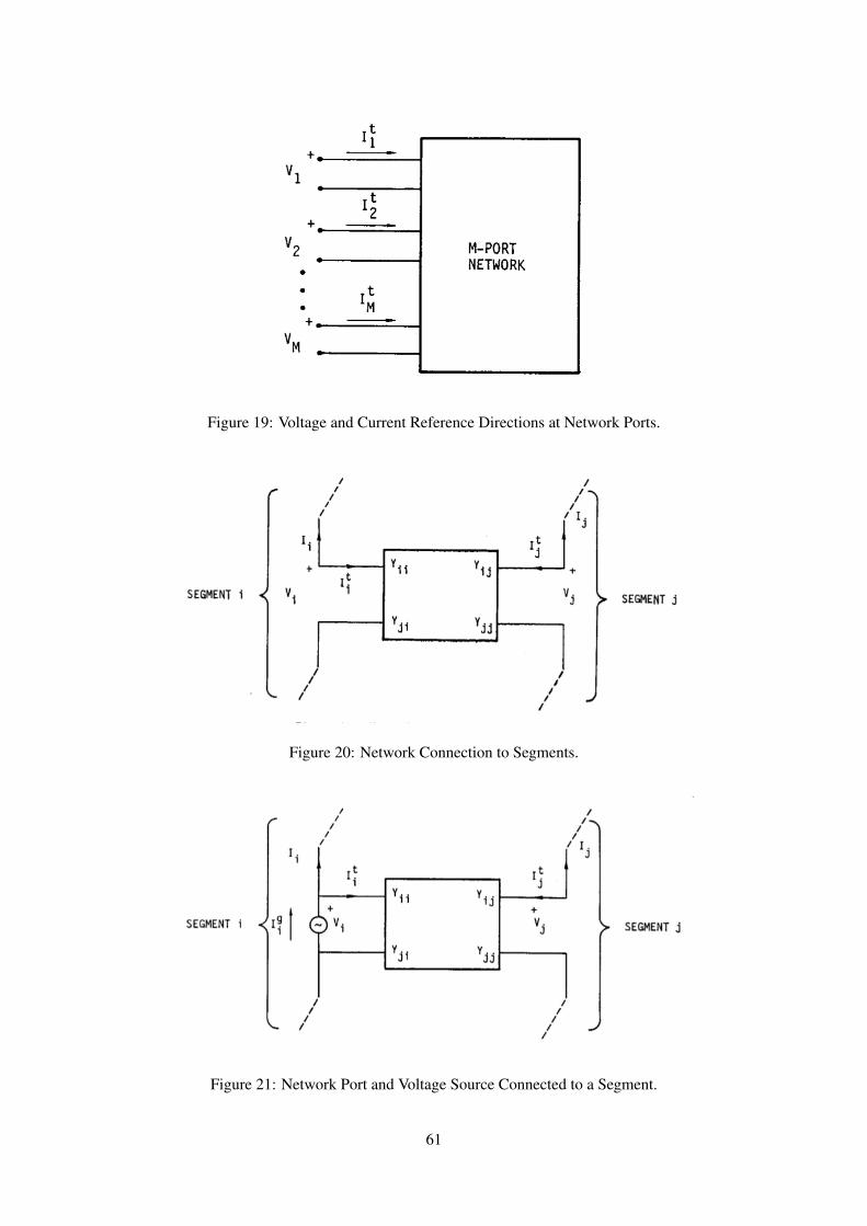
Figure 19: Voltage and Current Reference Directions at Network Ports.

Figure 20: Network Connection to Segments.

Figure 21: Network Port and Voltage Source Connected to a Segment.

61

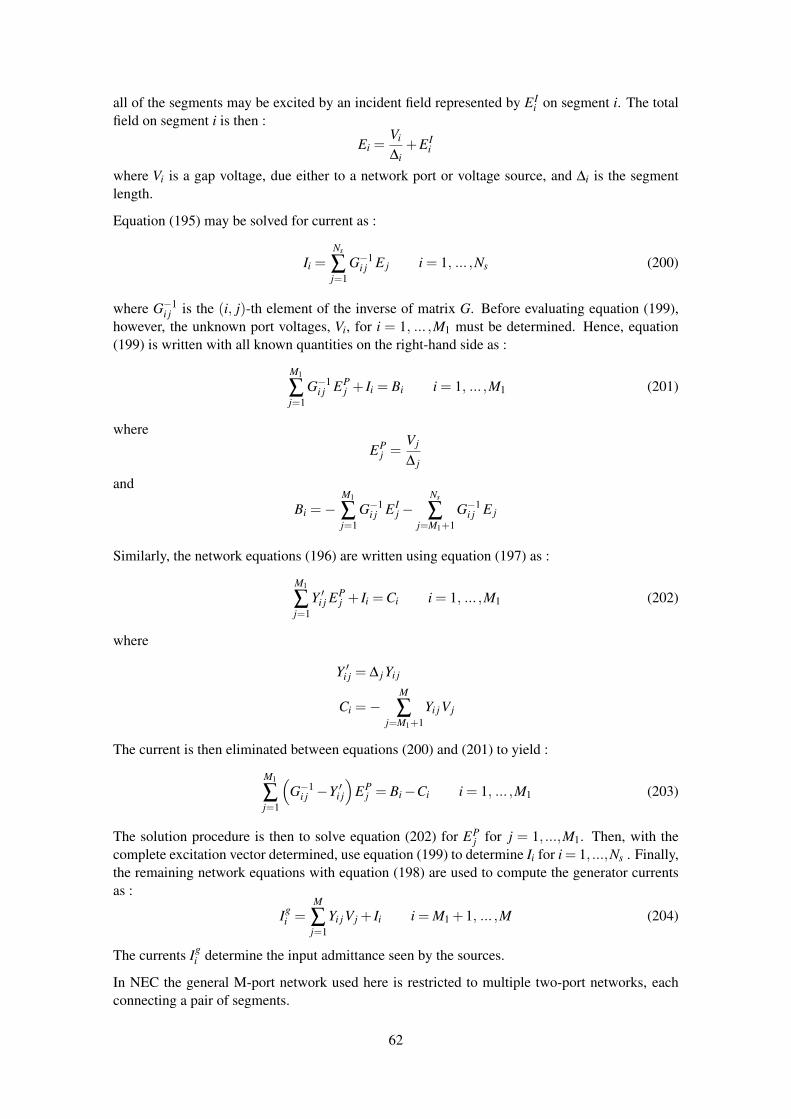
all of the segments may be excited by an incident field represented by E Ii on segment i. The total

field on segment i is then :

Ei =Vi

∆i+E I

i

where Vi is a gap voltage, due either to a network port or voltage source, and ∆i is the segmentlength.

Equation (195) may be solved for current as :

Ii =Ns

∑j=1

G−1i j E j i = 1, ... ,Ns (200)

where G−1i j is the (i, j)-th element of the inverse of matrix G. Before evaluating equation (199),

however, the unknown port voltages, Vi, for i = 1, ... ,M1 must be determined. Hence, equation(199) is written with all known quantities on the right-hand side as :

M1

∑j=1

G−1i j EP

j + Ii = Bi i = 1, ... ,M1 (201)

whereEP

j =Vj

∆ j

and

Bi =−M1

∑j=1

G−1i j E I

j−Ns

∑j=M1+1

G−1i j E j

Similarly, the network equations (196) are written using equation (197) as :

M1

∑j=1

Y ′i j EPj + Ii =Ci i = 1, ... ,M1 (202)

where

Y ′i j = ∆ j Yi j

Ci =−M

∑j=M1+1

Yi j Vj

The current is then eliminated between equations (200) and (201) to yield :

M1

∑j=1

(G−1

i j −Y ′i j

)EP

j = Bi−Ci i = 1, ... ,M1 (203)

The solution procedure is then to solve equation (202) for EPj for j = 1, ...,M1. Then, with the

complete excitation vector determined, use equation (199) to determine Ii for i = 1, ...,Ns . Finally,the remaining network equations with equation (198) are used to compute the generator currentsas :

Igi =

M

∑j=1

Yi j Vj + Ii i = M1 +1, ... ,M (204)

The currents Igi determine the input admittance seen by the sources.

In NEC the general M-port network used here is restricted to multiple two-port networks, eachconnecting a pair of segments.

62

5.3 Transmission Line Modeling

Transmission lines interconnecting parts of an antenna may be modeled either explicitly by includ-ing the transmission 1ine wires in the thin-wire model, or implicitly by the method described in thepreceding section for nonradiating networks. For an implicit model, the short-circuit-admittanceparameters of the transmission line viewed as a two-port network are :

Y11 = Y22 =− jY0 cot(kl)

Y12 = Y21 = jY0 csc(kl)

where Y0 is the characteristic admittance of the line, k is the wave number (2π/λ ), and l is thelength of the 1ine. If a separate admittance element is connected across the end of a transmission1ine, its admittance is added to the self-admittance of that network port.

The implicit model is limited, however, in that it neglects interaction between the transmissionline and the antenna and its environment. This approximation is justified if the currents in theline are balanced, ie. in a log periodic dipole antenna, and in general if the transmission linelies in an electric symmetry plane. The balance can be upset, however if the transmission line isconnected to an unbalanced load or by unsymmetric interactions. If the unbalance is significant,the transmission line can be modeled explicitly by including the wires in the thin-wire model.The explicit model is completely general, and yields accurate results since the sine, cosine, andconstant current expansion in NEC is a good representation of the sinusoidal transmission linecurrents. The accuracy is demonstrated in figure 22 for transmission lines terminated in shortcircuit, open circuit, and matched loads.

The explicit transmission line model is, of course, less efficient in computer time and storage be-cause of the additional segments required. In cases where the physical line presence does have asignificant effect on the results, the effect may be modeled by explicitly modeling a single con-ductor of the line while using the implicit model to represent the balanced current component.

63

Figure 22: Current Distribution on a Two-Wire Transmission Line from NEC Compared with theIdeal Transimission Line Solution.

64

5.4 Lumped or Distributed Loading

Thus far, we have assumed that all structures to be modeled are perfect electric conductors. TheEFIE is easily extended to imperfect conductors by modifying the boundary condition from equa-tion (4) to :

n(~r )×[~ES(~r )+~E I(~r )

]= Zs(~r )

[n(~r )× ~JS(~r )

]where ZS(~r ) is the surface impedance at ~r on the conducting surface. For a wire, the boundarycondition is :

s ·[~ES(~r )+~EI(~r )

]= Zw(s) I(s)

with |vecr and s the position vector and tangent vector at s on the wire and Zw(s) the impedanceper-unit-length at s. The matrix equation can then be written :

Ns

∑j=1

Gi j α j =−Ei +Zi

∆iIi i = 1, ... ,Ns (205)

where

α j = amplitude of basis function j

Ei = incident field on segment i

Ii = current at the center of segment i

Zi = total impedance of segment i

∆i = length of segment i

The impedance term can be viewed as a constant field model of a voltage source, as described insection V-1, where the voltage is proportional to current. It is assumed that the current is essentiallyconstant, with value Ii, over the length of the segment, which is a reasonable assumption for theelectrically short segments used in the integral equation solution.

The impedance term can be combined with the matrix by expressing Ii in terms of the α j as :

Ii =Ns

∑j=1

α j(Ai

j +Cij)

where Aij and Ci

j are the coefficients of the constant and cosine terms, respectively, in the sectionof basis function j extending onto segment i. If basis function j does not extend onto segment i,then Ai

j and Cij are zero. The matrix equation modified by loading is then :

Ns

∑j=1

G′i j α j =−Ei i = 1, ... ,Ns (206)

whereG′i j = Gi j−

Zi

∆i

(Ai

j +Cij)

(207)

For a lumped circuit element, Zi is computed from the circuit equations. Whereas for a distributedimpedance, Zi represents the impedance of a length ∆i of wire, which in the case of a round wireof finite conductivity is given by :

Zi =j∆i

aisqrt

ωµ

2πσ

[Ber(q)+ jBei(q)Ber′(q)+ jBei′(q)

]

65

where

q = aisqrtωµσ

ai = wire radius

σ = wire conductivity

Ber, Bei = Kelvin functions

This expression takes account of the limited penetration of the field into an imperfect conductor.

66

5.5 Radiated Field Calculation

The radiated field of an antenna or re-radiated field of a scatterer can be computed from the inducedcurrent by using a simplified form of equation (1) valid far from the current distribution. The far-field approximation valid when the distance from the current distribution to the observation pointis large compared to both the wavelength and the dimensions of the current distribution, treats thedistance |~r−~r ′| as constant integral except in the phase term, exp(− jk|~r−~r ′|). For a structureconsisting of a wire portion with contour L and current distribution I(s), and a surface portion Swith current ~Js(~r) , the far-zone field is :

~E(~ro) =jkη

4π

exp(− jkro)

ro

∫L

[(k ·~I(s)

)k−~I(s)

]exp( j~k ·~r )ds

+∫

S

[(k · ~Js(~r )

)k− ~Js(~r )

]exp( j~k ·~r )dA

(208)

where ~ro is the position of the observation point k =~ro/|~ro|, k = 2π/λ , and k = kk. The firstintegral can be evaluated in closed form over each straight wire segment for the constant, sine, andcosine components of the basis functions, and reduces to a summation over the wire segments.With the surface current on each patch represented by a delta function at the patch center, thesecond integral becomes a summation over the patches.

The radiation pattern of an antenna can be computed by exciting the antenna with a voltage sourceand using equation (207) to compute the radiated field for a set of directions in space. Alterna-tively, since the transmitting and receiving patterns are required by reciprocity to be the same,the pattern can be determined by exciting the antenna with plane-waves incident from the samedirections and computing the currents at the source point. The solution procedure in NEC doesnot guarantee reciprocity, however, since the different expansion and weighting functions mayproduce asymmetry in the matrix. Large differences between the receiving and transmitting pat-terns or a significant lack of reciprocity in bistatic scattering are indications of inaccuracy in thesolution, possibly from too coarse a segmentation of the wires or surfaces.

The power gain of an antenna in the direction specified by the spherical coordinates (θ ,φ) isdefined as :

GP(θ ,φ) = 4πP(θ ,φ)

Pin

where P(θ ,φ) is the power radiated per unit solid angle in the direction (θ ,φ), and Pin is the totalpower accepted by the antenna from the source. Pin is computed from the voltage and current atthe source as :

Pin =12

Re(V I∗)

and

P(θ ,φ) =12

R2 Re(~E× ~H∗)

=R2

2η(~E ·~E∗)

~E is obtained from equation (207) with~ro in the direction (θ ,φ), and ro = R. Directive gain issimilarly defined as :

Gd(θ ,φ) = 4πP(θ ,φ)

Prad

67

where Prad is the total power radiated by the antenna :

Prad = Pin−Ploss

and Ploss is the total ohmic loss in the antenna.

The radiated field of an antenna over ground is modified by the ground interaction, as discussedin Section IV. When the range from the antenna to the observer, R, approaches infinity, the Som-merfeld formulation for the field reduces exactly to a direct field determined by equation (207)and a field from the image modified by the Fresnel reflection coefficient. In some cases, however,when the observer is at a finite distance from the antenna, the field components proportional to1/R2 may be significant. While the 1/R terms are generally much larger than the 1/R2 terms atpractical observation distances from an antenna, the 1/R terms vanish at grazing angles over animperfect ground plane leaving only the 1/R2 terms, dominated by a term known as the groundwave. The ground wave is, of course, included in Sommerfeld’s expressions. Norton’s asymptoticapproximations (ref. 26) are used, however since they are more easily evaluated and give adequateaccuracy. Norton’s formulas, which are in Part II of this manua1 under subroutine GWAVE, arevalid for R greater than a few wavelengths and to second order in k2

1/k22. When the ground wave

is included, the field has radial as well as transverse components.

68

5.6 Antenna Coupling

Coupling between antennas is often a parameter of interest, especially when a receiving systemmust be protected from a nearby transmitter. Maximum power transfer between antennas occurswhen the source impedance and receiver load impedance are conjugate-matched to their antennas.Determination of this condition is complicated by the antenna interaction, however, since the inputimpedance of one antenna depends on the load connected to the other antenna. NEC-2 includes analgorithm for determining the matched loads and maximum coupling by a method that was addedto special versions of the previous codes NEC-1 and AMP (ref. 34).

The coupling problem can be solved in closed form by the Linville method (ref. 35), a techniqueused in RF amplifier design. The first step is to determine the two-port admittance parameters forthe coupled antennas by exciting each antenna with the other short-circuited and computing theself and mutual admittances from the currents computed by NEC. The maximum coupling is then :

GMAX =1L

[1−√

1−L2]

where

L =|Y12Y21|

2Re(Y11)Re(Y22)−Re(Y12Y21)

The matched load admittance on antenna 2 for maximum coupling is :

YL =

[1−ρ

1+ρ+1]

Re(Y22)−Y22

where

ρ =GMAX(Y12Y21)

∗

|Y12Y21|and the corresponding input admittance of antenna 1 is :

YIN = Y11−Y21Y12

YL +Y22

69

References

[1] Miller, E. K. et al, Final Technical Report of the Log-Periodic Scattering Array Program,MBAssociates Report No. MB-R-70/l05, Contract No. F04J0l-68-C-0188, 1970.

[2] RCS Computer Program BRACT, Log-Periodic Scattering Array Program - II, MBAs-sociates Report No. MB-R-69/46, Contract No. F0470l-68-C-0188, 1969.

[3] Antenna Modeling Program - Composite User’s Manual, MBAssociates Report No. MB-R-74/46, 1974.

[4] Antenna Modeling Program - Engineering Manual, MBAssociates Report No. MB-R-74/62, 1974.

[5] Antenna Modeling Program - Systems Manual, MBAssociates Report No. MB-R-74/62,1974.

[6] Antenna Modeling Program - Supplementary Computer Program Manual (AMP2),MBAssociates Report No. MB-R-74/62, l975.

[7] Numerical Electromagnetic Code (NEC-1) Part III: NEC User’s Guide, Lawrence Liv-ermore Laboratory, 1977.

[8] Numerical Electromagnetic Code (NEC-1) Part II: NEC Program Description - Code,Lawrence Livermore Laboratory, 1977.

[9] Albertsen, N. C., Hansen, J. E., and Jensen, N. E., Computation of Spacecraft AntennaRadiation Patterns, The Technical University of Denmark, Lyngby, Denmark, June 1972

[10] Poggio, A. J. and Miller, E. K., Integral Equation Solutions of Three Dimensional Scat-tering Problems, Chapt. IV in Computer Techniques for Electromagnetics, edited by R.Mittra, Pergamon Press, New York, l973.

[11] Poggio, A. J. and Adams, R. W., Approximations for Terms Related to the Kernel in Thin-wire Integral Equations, UCRL-51985, Lawrence Livermore Laboratory, CA, December19, l975.

[12] Van Bladel, J., Electromagnetic Fields, McGraw-Hill, New York, 1964.

[13] Harrington, R. F., Field Computation by Moment Methods, MacMi11an, New York, 1968.

[14] Yeh, Y. S. and Mei, K. K., Theory of Conical Equiangular Spiral Antennas, PartI -Numerical Techniques, IEEE Trans. Ant. and Prop., AP-15, 1967, p. 634.

[15] Neureufher, A. R. et al, A Comparison of Numerical Methods for Thin Wire Antennas,Presented at the 1968 Fall URSI Meeting, Dept. of Electrical Engineering and ComputerSciences, University of California Berkeley, 1968.

[16] Miller, E. K. et al, An Evaluation of Computer Programs Using Integral Equations forthe Electromagnetic Analysis of Thin Wire Structures, UCRL-75566, Lawrence Liver-more Laboratory, CA, March 1974.

[17] Wu, T. T. and King, R. W. P., The Tapered Antenna and Its Application to the JunctionProblem for Thin Wires, IEEE Trans. Ant. and Prop., AP-24, No. 1, pp. 42-45, January1976.

70

[18] Poggio, A. J., Integral Representations for Fields Due to Sources on Open Surfaces withApplications to End Caps, UCRL-51723, Lawrence Livermore Laboratory, CA, December16, 1974.

[19] Ralston, A., A First Course in Numerical Analysis, McGraw-Hill, New York, 1965.

[20] Sommerfeld, A., Partial Differential Equations in Physics, Academic Press New York,1964.

[21] Burke, G. J., Miller, E. K., and Poggio, A. J., Dielectric Ground Interactions with a Log-Periodic Antenna, Final Report, ECOM-0285-F, U.S. Army Electronics Command, FortMonmouth, N.J., 1972 (contract DAAB07-70-C-0285).

[22] Mi1ler, E. K., Poggio, A. J., Burke, G. J., and Selden, E. S., Analysis of Wire Antennas inthe Presence of a Conducting Half Space: Part I. The Vertical Antenna in Free Space.Part II. The Horizontal Antenna in Free Space, UCRL-732l7, Lawrence Livermore Lab-oratory, CA, 1972. (Also in Canadian J. Phys.)

[23] Lager, D. L. and Lytle, R. J., Fortran Subroutines for the Numerical Evaluation of Som-merfeld Integrals Unter Anderem, UCRL-51821, Lawrence Livermore Laboratory, CA,May 21, 1975.

[24] Adams, R. W., Poggio, A. J., and Miller, E. K., Study or a New Antenna Source Model,UCRL-51693, Lawrence Livermore Laboratory, CA, October 28, 1974.

[25] Brittingham, J. M., Miller, E. K., and Okada, J. T., SOMINT: An Improved Model forStudying Conducting Objects Near Lossy Half-Spaces, UCRL-52423, Lawrence Liver-more Laboratory, CA, February 24, 1978.

[26] Norton, K. A., The Propagation or Radio Waves Over the Surface of the Earth and inthe Upper Atmosphere, Proceedings of the Institute of Radio Engineers, Vol, 26, No. 9,Sept. 1937.

[27] Lytle, R. J. and Lager, D. L., Numerical Evaluation of Sommerfeld Integrals, UCRL-51688, Lawrence Livermore Laboratory, CA, October 23, 1974.

[28] Shanks, D., Non-Linear Transformations of Divergent and Slowly Convergent Se-quences, J. Math. Phys., 24, 1 (1955).

[29] Miller, E. K. and Deadrick, F. J., Computer Evaluation of Loran-C Antennas, UCRL-51464, Lawrence Livermore Laboratory, CA, Oct. 17, l973.

[30] Wait, J. R., Characteristics of Antennas Over Lossy Earth, Antenna Theory, Part II, R.E. Collin and F. J. Zucker, Eds., McGraw-Hill, New York, pp. 386-437, 1969.

[31] King, R. W., The Theory of Linear Antennas, Harvard Univ. Press Cambridge, Mas-sachusetts, 1956.

[32] Otto, D. V., The Admittance of Cylindrical Antennas Driven From a Coaxial Line, RadioSci., Vol. 2, No. 9, pp. 1031-1042, 1967.

[33] Andreasen, M. G. and Harris, P. G., Analyses of Wire Antennas of Arbitrary Configura-tion by Precise Theoretical Numerical Techniques, Tech. Rept. ECOM 0631-F, GrangerAssociates, Palo Alto, CA, Contract DAAB07-67-0631, 1968.

[34] Logan, J. C, and Rockway, M. W., Computer Techniques for Shipboard Topside AntennaModeling Below UHF, TN-3284, Naval Electronics Laboratory Center, November 17, 1976.

71

[35] Rubin, D., The Linville Method of High Frequency Transistor Amplifier Design, NavalWeapons Center, Research Department, NWCCL TP 845, Corona Laboratories, Corona, CA,March 1969.

[36] Burke, G. J., and Poggio, A. J., Computer Analysis of the Twin-Whip Antenna, UCRL-52080, Lawrence Livermore Laboratory, CA, June 1, l976.

[37] Burke, G. J. and Poggio, A. J., Computer Analysis of the Bottom-Fed Fan Antenna,UCRL-52109 Lawrence Livermore Laboratory, CA, August 19, 1976.

[38] Deadrick, F. J., Burke, G. J., and Poggio, A. J., Computer Analysis of the Trussed-Whipand Discone-Cage Antennas, UCRL-52201, January 6, 1977.

72