Go Ahead, Be Prepared: Comparing Multivariate Models for

Evaluating the Math Plus Intervention Stephen Blohm, Leila Jamoosian, Megan Leonard,

Terra Morris, and Terrence Willett

RP Conference: Burlingame, CA April 21, 2017

y = f(x)

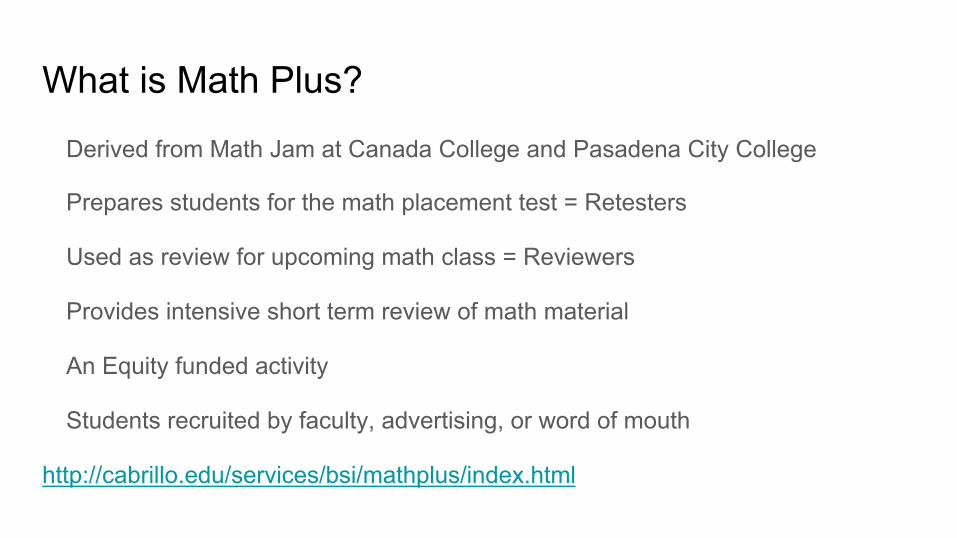
What is Math Plus?

Derived from Math Jam at Canada College and Pasadena City College

Prepares students for the math placement test = Retesters

Used as review for upcoming math class = Reviewers

Provides intensive short term review of math material

An Equity funded activity

Students recruited by faculty, advertising, or word of mouth

http://cabrillo.edu/services/bsi/mathplus/index.html

Research Questions

Does MathPlus work?

Does it reduce disproportionate impacts?

Possible outcome measures

1. Level of placement

2. Percent of students who enroll in math immediately after assessment

3. Success in given level of math

4. Throughput to completion of a target level of math

5. Impact on self-efficacy

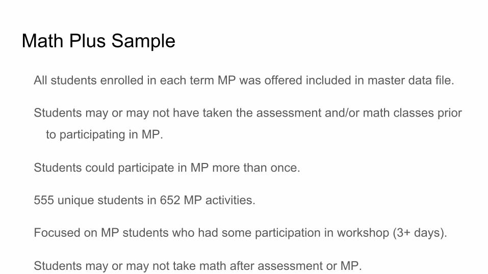
Math Plus Sample

All students enrolled in each term MP was offered included in master data file.

Students may or may not have taken the assessment and/or math classes prior

to participating in MP.

Students could participate in MP more than once.

555 unique students in 652 MP activities.

Focused on MP students who had some participation in workshop (3+ days).

Students may or may not take math after assessment or MP.

Data File

51,977 records from 4 primary terms in 2015 and 2016

6 cohorts of Math Plus cohorts ranging from 43 to 177 students

148 variables

~1.3 gazillion lines of code

The 3 Stages of IR

MP (3+ days) v. non-MP Student Characteristics Elem Alg Int Alg

MP non-MP MP non-MP

Count 83 1,992 145 2,970

Pre-MP GPA 3.23 2.51 3.01 2.59

Pre-MP Units 37.9 35.8 48.6 38.7

% First Time 40% 23% 26% 25%

% Female 59% 55% 63% 53%

% URM 69% 64% 61% 61%

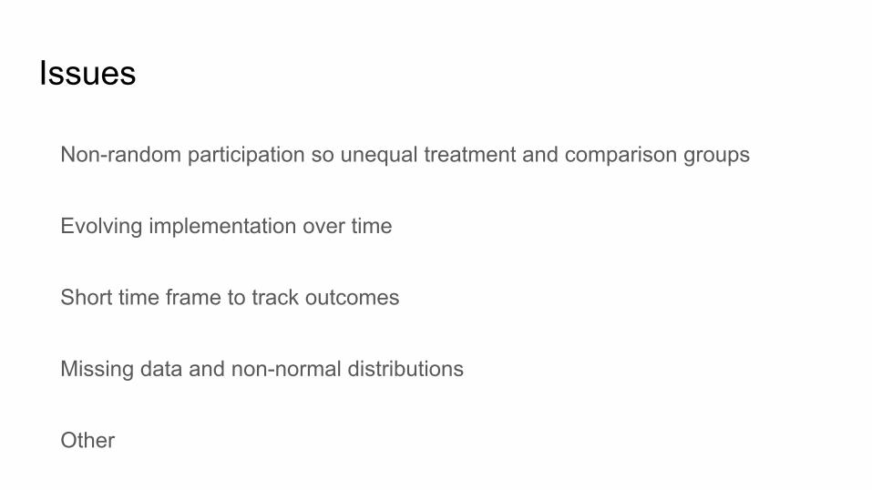
Issues

Non-random participation so unequal treatment and comparison groups

Evolving implementation over time

Short time frame to track outcomes

Missing data and non-normal distributions

Other

Bar Chart

χ2 = 27.7564, p < 0.001

Exploration and Analysis Excel pivot table

𝝌2 analysis

PowerBI Data Visualization

Logistic Regression

Analysis of Covariance

Hierarchical Multiple Regression Analysis

Propensity Score Matching (PSM)

Classification and Regression Tree (CART)

Software

Excel

PowerBI

SPSS

STATA

R (make sure you have sufficient RAM)

Power BI Data Visualization

Power BI Data Visualization

What is Logistic Regression? One or more dependent variables or predictors estimating probability of a binary

outcome

Uses logit link function(why not probit?)

Standard IR analysis technique

Interpret using 𝛽 coefficients, odds ratios, and marginal means

Cox, DR (1958). "The regression analysis of binary sequences (with discussion)". J Roy Stat Soc B. 20: 215–242.

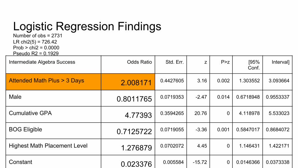
Logistic Regression Findings Number of obs = 2731 LR chi2(5) = 726.42 Prob > chi2 = 0.0000 Pseudo R2 = 0.1929

Intermediate Algebra Success Odds Ratio Std. Err. z P>z [95% Conf.

Interval]

Attended Math Plus > 3 Days 2.008171 0.4427605 3.16 0.002 1.303552 3.093664

Male 0.8011765 0.0719353 -2.47 0.014 0.6718948 0.9553337

Cumulative GPA 4.77393 0.3594265 20.76 0 4.118978 5.533023

BOG Eligible 0.7125722 0.0719055 -3.36 0.001 0.5847017 0.8684072

Highest Math Placement Level 1.276879 0.0702072 4.45 0 1.146431 1.422171

Constant 0.023376 0.005584 -15.72 0 0.0146366 0.0373338

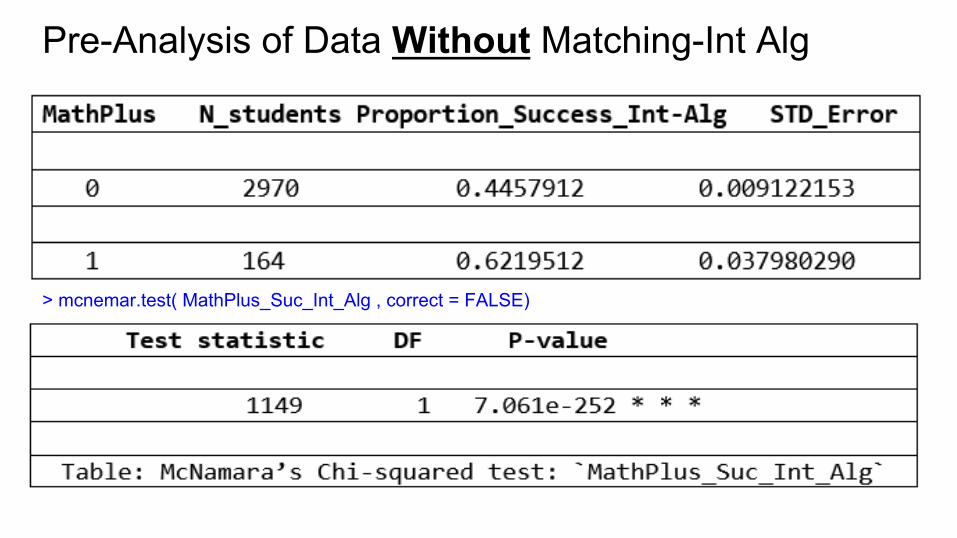
Pre-Analysis of Data Without Matching-Int Alg

> mcnemar.test( MathPlus_Suc_Int_Alg , correct = FALSE)

Logistic Regression Outcome by R - Int Alg > summary(gl_152)

Continue: Logistic Regression Findings by R - Int Alg Taking rest of variables as constant, ●  For student who participate in Math

Plus, the odds ratio of success in Int-Alg is 1.59 times greater who did not participate (base-line Math-Plus).

●  Being eligible for BOG, vs. not being eligible, decrease the odd ratio of success in Int-Alg by 0.78 (base-line eligible for BOG).

●  The odd ratio of success in Int-Alg for male is 0.79 less than female (base-line is female).

●  Students in transfer level placement, versus students who are in lowest placement level (-4) changes the odds ratio of Math Plus students success by 2.97 (base-line is -4 lowest level).

●  For every one unit increase in GPA, the odds of success in Int Alg increase 4.3.

> Odds_Ratio=exp(coef(gl_152)) > conInt=confint(gl_152)

Model Selection Methods

“All models are wrong, but some are useful.” by George Box

We are not finding the “correct” model, but rather trying to solve our practical problems using a model reasonable for our purposes.

BIC (Bayesian Information Criterion): BIC=k* log(n) - 2 log(L)

AIC (Akaike Information Criterion): AIC=2k - 2 log(L)

R-Square & Adjusted R-Square : Does not apply to logistic regression models - there is trick

Predictors Selection by “LEAP” (Included all)

Predictors Selection by “LEAP” (Final Covariates)

Pre-Analysis of Data Without Matching- Elem Alg

What is PSM? Based on counterfactual theories of causation by philosopher David Lewis

Rosenbaum, P. R., & Rubin, D. B. (1983). The central role of the propensity score in observational studies for causal effects. Biometrika, 70, 41-55.

Key unobservable questions:

What would MP student success have been if they had not participated in MP?

What would non-MP student outcomes have been if they had been in MP?

Calculate probability that non-MP student would have been in MP based on their background characteristics to create comparison group

Interpret effect size of Average Treatment Effect (ATE) or Average Treatment Effect on the Treated (ATT)

Best for small samples with few variables

It is NOT universally superior to other methods

Analysis of Data after Matching and ATE by “MachIt”

Math Plus Success Rate After PSM- Int Alg

STATA - psmatch2 Propensity Score Matching . psmatch2 MathPlus_Attend1 Gender_num BOG_Elg GPA_Cum HighestMathPlacementLevel if m152interm==1, out ( m152intermSuc) ate

Probit regression Number of obs = 2731 Pseudo R2 = 0.0395

-----------------------------------------------------------------------------------------------------------------------------------------------

Variable Sample | Treated Controls Difference S.E. T-stat

----------------------------+-----------------------------------------------------------------------------------------------------------------

m152intermSuc Unmatched | .6796875 .445255474 .234432026 .044886811 5.22

ATT | .6796875 .5390625 .140625 .064749091 2.17

ATU | .4452554 .565885517 .120630042

ATE | .121567192

. teffects psmatch (m152intermSuc) (MathPlus_Attend1 Gender_num BOG_Elg GPA_Cum HighestMathPlacementLevel) if m152interm==1 Treatment-effects estimation Number of obs = 2731 Estimator : propensity-score matching Matches: requested = 1 Outcome model : matching min = 1 Treatment model: logit max = 24 ----------------------------------------------------------------------------------------------------------------------------------- AI Robust m152intermSuc Coef. Std. Err. z P>|z| [95% Conf. Interval] -----------------+---------------------------------------------------------------------------------------------------------------- ATE MathPlus_Attend1 (1 vs 0) .140815 .0693769 2.03 0.042 .0048387 .2767912

STATA - teffects Propensity Score Matching

PSM Machine Learning with “twang” package in R http://www.rand.org/statistics/twang/r-tutorial.html

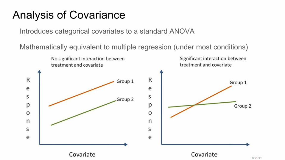
Analysis of Covariance Introduces categorical covariates to a standard ANOVA

Mathematically equivalent to multiple regression (under most conditions)

Analysis of Covariance- MP Analysis

Data: Students who took Math 152 Dependent Variable: Grade points in Math 152 Independent Variable: Math Plus Participation

Covariates: - Cumulative GPA - BOG Eligible - Gender - Highest Math Placement

Analysis of Covariance- Results Source Type III SS df Mean Square F Sig

Corrected Model 1610.52 5 322.11 285.90 <.001

Intercept 34.58 1 34.58 30.69 <.001

Highest Placement 34.79 1 34.79 30.88 <.001

Cumulative GPA 1524.89 1 1524.89 1353.48 <.001

BOG Eligible 9.17 1 9.17 8.14 0.004

Gender 0.32 1 0.32 0.28 0.594

Math Plus 7.06 1 7.06 6.27 0.012

Error 2338.92 2076 1.13

Total 10776.00 2082

Corrected Total 3949.44 2081 R2 = .408 (adjusted R2 = .406)

Hierarchical Multiple Regression Analysis

Adds variables to the model in stages

Change in R2 is calculated (vs ANCOVA where only total R2 is calculated)

Hypothesis test is done to test whether the change in R2 in the second step is

significantly different from 0

Demographic variables can go in the first step to hold them constant, then

change in R2 can be calculated to determine how much of an effect a

predictor (Math Plus) has on the outcome variable (grade points in Math 152)

Hierarchical Multiple Regression- MP Analysis Data: Students who took Math 152 Dependent Variable: Grade points in Math 152

Step 1 Independent Variables*: - Cumulative GPA - BOG Eligible - Gender - Highest Math Placement

Step 2 Independent Variables: - Math Plus

* several models were run and results were very similar when additional demographic variables were entered in step 1

Hierarchical Multiple Regression- Correlation Matrix

Grade Points Gender Highest Math Cumulative GPA

BOG Eligible Math Plus

Grade Points 1.00 - 0.08*** 0.04* 0.63*** - 0.05** 0.10***

Gender 1.00 0.14*** - 0.14*** - 0.08*** - 0.06**

Highest Math 1.00 - 0.10*** - 0.19*** - 0.01

Cumulative GPA 1.00 0.02 0.10***

BOG Eligible 1.00 0.07***

Math Plus 1.00

p<0.05 = * p<0.01 = ** p<0.001 = ***

Hierarchical Multiple Regression- Model Summary

Overall R2 shows a small effect, but when holding demographics constant in the first step, ΔR2 for the second step shows a very small effect (ΔR2 = .006), though both steps remain statistically significant.

Model R R2 Adj R2 Std Er ΔR2 ΔF df1 df2 ΔF sig

1 .637 .406 .405 1.063 .406 354.91 4 2077 <.001

2 .639 .408 .406 1.061 .002 6.27 1 2076 .012

What are Decision Trees? •  Howard Raiffa explains decision trees in Decision

Analysis (1968). •  Ross Quinlan invented ID3 and introduced it to the world

in his 1975 book, Machine Learning. •  CART popularized by Breiman et al. in mid-90’s

–  Breiman, L., Friedman, J., Olshen, R., & Stone, C. (1994). Classification and regression trees. Chapman and Hall: New York, New York.

–  Based on information theory rather than statistics; developed for signal recognition

   How  is  homogeneity  measured?  

●  Gini-­‐Simpson  Index  ●  p-­‐square  =  probability  of  two  items  taken  at  random  from  the  set  being  of  

same  types;  D=dissimilarity/diversity  ●  Proposed  by  Corrado  Gini  in  1912  as  a  measure  of  inequality  of  income  or  

wealth;  used  in  demographics  and  ecology  as  diversity  index  ●  If  selecJng  two  individual  items  randomly  from  a  collecJon,  what  is  the  

probability  they  are  in  different  categories.  ●  Other  indices  such  as  Shannon-­‐Wiener  can  also  be  used  

Pros  and  Cons  of  Decision  Trees    Strengths  •  VisualizaJon  •  Easy  to  understand  output  •  Easy  to  code  rules  •  Model  complex  relaJonships  

easily  •  Linearity,  normality,    not  

assumed    •  Handles  large  data  sets  •  Can  use  categorical  and  

numeric  inputs    

Weaknesses  •  Results  dependent  on  training  

data  set  –  can  be  unstable  esp.  with  small  N  

•  Can  easily  overfit  data  •  Out  of  sample  predicJons  can  

be  problemaJc  •  Greedy  method  selects  only  

‘best’  predictor  •  Must  re-­‐grow  trees  when  

adding  new  observaJons  

Intermediate Algebra Success: split, n, deviance, yval * denotes terminal node 1) root 3115 2230.59600 0.4561798 2) GPA_Pre< 2.855 2301 1677.89100 0.4181154 4) Latino_num>=0.5 1333 980.72330 0.3714821 8) Math154_Attemtps>=2.5 85 54.73815 0.2064407 * 9) Math154_Attemtps< 2.5 1248 917.46070 0.3831411 18) MathPlus< 0.5 1192 876.95630 0.3726369 * 19) MathPlus>=0.5 56 33.93440 0.6014560 * 5) Latino_num< 0.5 968 680.79520 0.4823787 10) HighestMathPlacementLevel< -2.5 74 53.37814 0.3018685 * 11) HighestMathPlacementLevel>=-2.5 894 620.89200 0.4976611 22) Gender_num>=0.5 497 359.99060 0.4347024 * 23) Gender_num< 0.5 397 251.99840 0.5761637 * 3) GPA_Pre>=2.855 814 525.93160 0.5635928 6) GPA_Pre< 3.615 540 372.42520 0.5053559 * 7) GPA_Pre>=3.615 274 144.10720 0.6770649 *

Comparative Findings for Intermediate Algebra Method Conclusion Effect Size

Bar charts MP works 22 points

Visualization MP works MP students did better in Math 152 than non MP students

Logistic Regression MP sort of works OR = 2 (STATA), OR=1.6 (R)

PSM MP might work Matching=0.3 Matchit = 0.15 psmatch2 = 0.12 teffects = 0.14 twang = 0.06

ANCOVA MP sort of works R2 = 0.408; MP is significant

Hierarchical MRC MP doesn’t work that well ΔR2 = 0.002; MP is significant

Decision Trees MP works for a subset R2=0.04

Conclusions

MathPlus may be effective for increasing success rates in Intermediate Algebra

to a statistically and practically significant degree

Results were not generally significant for Elementary Algebra success rates

Initial recommendations will center of recruitment strategies

Limitations and Next Steps

Self-selection bias

Data distribution issues for some analyses

Limited time to track outcomes

Different methods show different effect sizes

Some models more sensitive to variables included in model

Various techniques have varying underlying assumptions

Researchers from different disciplines have different approaches

Each software package offers different options

Next will examine self-efficacy data from surveys

Thank you

A statistician, an economist, a social psychologist, an experimental psychologist, and an ecologist walk into a bar... The ecologist offers a free beer to the others. The economist says there is no such thing as a free beer but would like a pint of IPA. The statistician thinks they probably won’t actually pour 16 oz. The social psychologist hypothesizes that the variance under 16 oz will correlate to perceived social capital. The experimental psychologist suggests the bartender pour several replicates. The ecologist gets the bill and decides the economist was right. The statistician was right too. The social psychologist’s hypothesis was not confirmed as they had too much fun toasting the end of the presentation to measure the beer.