3/7/2016

1

Very Brief Overview of

Discriminant Function Analysis

Comparison to PCA

Goals of DFA

• To determine which variables discriminate

between two or more naturally occurring

groups

• To model a function that can be used to

predict membership in groups based on

measured variables

3/7/2016

2

Example

• The use of measurements of bones to decide group membership (eg, species of lizard). A set of bones from known groups is used to create the discriminant function. It is then applied to measurements of bones (where group membership is not known)

Iris flower morphology

Setosa Versicolor Viginica

Can species be discriminated based on:

-Petal Length

-Petal Width

-Sepal Length

-Sepal Width

3/7/2016

3

Bivariate groups

3D groupings

How to build a

function that

discriminates

groups using all

the information

3/7/2016

4

• Mathematically DFA is equivalent to MANOVA

• Model in MANOVA is

Y1, Y2… YN = X

Where Y’s are continuous and X is categorical and the

question is if Y’s are related to X

• Model in DFA is

X = Y1, Y2…YN

Where Y’s are continuous and X is categorical and the

question is if X can be predicted base on Y’s

DFA vs MANOVA

DFA vs PCA

• In DFA ordination of variables is made to

maximize discrimination of groups

• In PCA ordination of variables is made to

reduce the number of variables by

developing composite variables (from co-

linear variables)

– Done without respect to Groups

3/7/2016

5

Comparison of PCA to DFA –

worked example - PCA

• Collection of Fish from two locations (1 and 2)

• Measurement of Ba and Sr in the otoliths of each fish

– Like a recorder of water chemistry experienced by individuals over the course of their life

• Can PCA reduce the variables to a single composite variable

Otoliths

1) Earbones of fish

2) Mainly calcium carbonate

a) Replacement minerals from water body embedded in matrix

3) Inert – unchanging over time

4) Matrix is laid down constantly

5) Rings are laid down daily

a) Annual rings as well

b) Often a settlement check

3/7/2016

6

Relationship between Strontium

and Barium – obvious colinearity

0 1 2 3 4 5 6 7 8 9 10

BARIUM

0

5

10

15

20

ST

RO

NT

IUMEach dot is a fish

Relationship between Strontium

and Barium – use of PCA

0 1 2 3 4 5 6 7 8 9 10

BARIUM

0

5

10

15

20

ST

RO

NT

IUM

-2 -1 0 1 2 3

PCA FACTOR1

Low Ba and Sr High Ba and Sr

Percent of Total Variance

Explained = 94%

3/7/2016

7

Good Fit?

-2 -1 0 1 2 3

PCA_FACTOR1

0

1

2

3

4

5

6

7

8

9

10

BA

RIU

M

-2 -1 0 1 2 3

PCA_FACTOR1

0

5

10

15

20

ST

RO

NT

IUM

Component loadings (relationship between

composite variable and original variables)

BARIUM 0.9707

STRONTIUM 0.9707

Comparison of PCA to DFA –

worked example -DFA

• Collection of Fish from two locations (1 and 2)

• Measurement of Ba and Sr in the otoliths of each fish – Like a recorder of water chemistry experienced by

individuals over the course of their life

• Can we build a function that will allow us to determine the locations of fish that are caught – discriminate locations of fish - of unknown origin – Use fish of known origin to build a model that predict

origin of those whose origin is unknown

Discriminant Function Analysis

3/7/2016

8

Relationship of Barium to Strontium

– no group membership

0 1 2 3 4 5 6 7 8 9 10

BARIUM

0

5

10

15

20

ST

RO

NT

IUM

Relationship of Barium to Strontium

– with group membership

0 1 2 3 4 5 6 7 8 9 10

BARIUM

0

5

10

15

20

ST

RO

NT

IUM

21

LOCATION

3/7/2016

9

Discrimination between sites – use

DFA

0 1 2 3 4 5 6 7 8 9 10

BARIUM

0

5

10

15

20

ST

RO

NT

IUM

2 1

LOCATION Ordinate to discriminate groups and

generate coefficients

Canonical discriminant function (coeficients)

Constant 1.3

BARIUM 0.95

STRONTIUM -0.69

Discrim Score = 1.3 + .95(Ba) -.69(Sr)

For each fish

LOCATION BARIUM STRONTIUM DISC_SCORE1

1 8.33 9.04 2.99

1 9.33 12.36 1.65

1 1.15 2.11 0.94

1 0.67 1.17 1.14

1 4.93 6.06 1.81

1 8.01 12.51 0.28

1 5.69 7.22 1.73

1 5.01 8.23 0.39

1 7.97 10.04 1.95

1 3.88 5.01 1.54

2 7.81 14.54 -1.31

2 0.10 3.20 -0.81

2 1.49 4.64 -0.48

2 0.30 3.43 -0.78

2 6.85 15.15 -2.65

2 6.58 11.03 -0.05

2 1.82 6.35 -1.35

2 4.39 8.07 -0.09

2 7.31 13.69 -1.20

2 9.62 13.86 0.89

Discrim Score = 1.3 + .95(8.33) -.69(9.04)

=2.99

Discrim Score = 1.3 + .95(Ba) -.69(Sr)

For each fish

3/7/2016

10

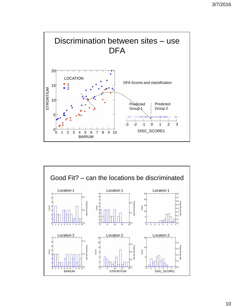
Discrimination between sites – use

DFA

0 1 2 3 4 5 6 7 8 9 10

BARIUM

0

5

10

15

20

ST

RO

NT

IUM

2 1

LOCATION DFA Scores and classification

-3 -2 -1 0 1 2 3

DISC_SCORE1

Predicted

Group 2 Predicted

Group 1

Good Fit? – can the locations be discriminated

0 1 2 3 4 5 6 7 8 9 10 0

1

2

3

4

5

6

7

Count

0.0

0.1

0.2

Pro

portio

n p

er B

ar

0 1 2 3 4 5 6 7 8 9 10

BARIUM

0

1

2

3

4

5

6

7

Count

0.0

0.1

0.2

Pro

portio

n p

er B

ar

0 5 10 15 20 0

1

2

3

4

5

6

7

8

9

Count

0.0

0.1

0.2

Pro

portio

n p

er B

ar

0 5 10 15 20

STRONTIUM

0

2

4

6

8

10

12

Count

0.0

0.1

0.2

0.3 Pro

portio

n p

er B

ar

-4 -3 -2 -1 0 1 2 3 0

5

10

15

20

25

Count

0.0

0.1

0.2

0.3

0.4

0.5

0.6

0.7

0.8

Pro

portio

n p

er B

ar

-4 -3 -2 -1 0 1 2 3

DISC_SCORE1

0

5

10

15

Count

0.0

0.1

0.2

0.3

0.4

Pro

portio

n p

er B

ar

Location 1 Location 1 Location 1

Location 2 Location 2 Location 2

3/7/2016

11

Good Fit? – classification matrices

and multivariate F and P

Classification matrix (cases in row categories classified into columns)

1 2 %correct

1 28 3 90

2 5 26 84

Total 33 29 87

Jackknifed classification matrix

1 2 %correct

1 27 4 87

2 5 26 84

Total 32 30 85

Pillai's trace= 0.602

Approx.F= 44.562 df= 2, 59 p-tail= 0.0000

0 1 2 3 4 5 6 7 8 9 10

BARIUM

0

5

10

15

20

2 1

LOCATION

0 1 2 3 4 5 6 7 8 9 10

BARIUM

0

5

10

15

20

ST

RO

NT

IUM

PCA ordination DFA ordination

Compare PCA to DFA

3/7/2016

12

-2 -1 0 1 2 3 PCA_FACTOR1

2 1

LOCATION

-4 -3 -2 -1 0 1 2 3 DISC_SCORE1

Compare PCA to DFA

Advanced topics

• Mahalanobis distance in DFA

• Linear vs quadratic based case

assignment

• Priors

3/7/2016

13

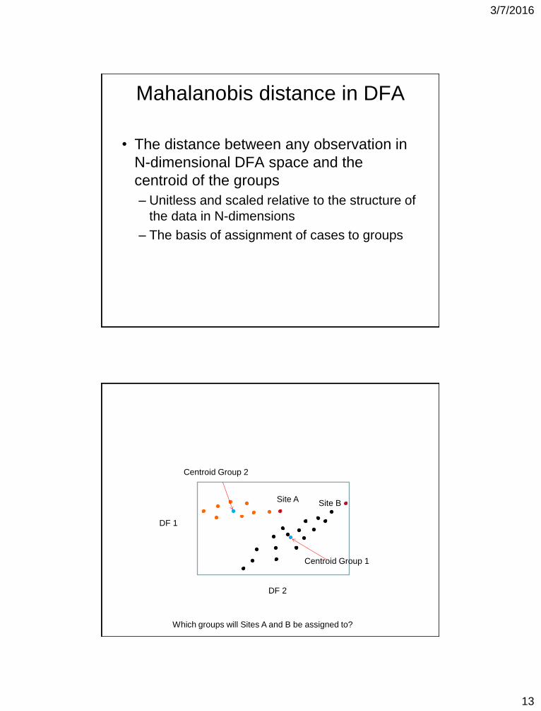
Mahalanobis distance in DFA

• The distance between any observation in

N-dimensional DFA space and the

centroid of the groups

– Unitless and scaled relative to the structure of

the data in N-dimensions

– The basis of assignment of cases to groups

DF 2

DF 1

Site A Site B

Centroid Group 1

Centroid Group 2

Which groups will Sites A and B be assigned to?

3/7/2016

14

Euclidean distances

Site A Site B

Euclidean assignment of

sites A and B

Distance 1B<2B, assign

to group 1

Distance 1A<2A assign

to group 1

Centroid Group 1

Centroid Group 2

DF 2

DF 1

Mahalanobis distances – consider covariance

(density) structure

Site A Site B

Centroid Group 1

Centroid Group 2

Now which groups will Sites A and B be assigned to?

DF 2

DF 1

3/7/2016

15

Classical vs Quadratic DFA

More generally, how should assignment be made?

2

1

LOCATION

-5 -4 -3 -2 -1 0 1 2 3 4 5

Discriminant Score

0

5

10

15

20

25

Count

Classical

Assignment based on linear distance between centroid and any observation

Assigned as

location 1 Assigned as

location 2

3/7/2016

16

2

1

LOCATION

-5 -4 -3 -2 -1 0 1 2 3 4 5

Discriminant Score

0

5

10

15

20

25

Count

Quadratic

Assignment based on probability density distance between centroid and any observation

Assigned as

location 1 Assigned as

location 2

Consider a two DF example

Quadratic will not always resolve but is considered to be more accurate

3/7/2016

17

Priors in DFA

• “Prior” refers to any probability of assignment that exists

(and that you want to incorporate) outside of the

analysis.

• For example lets say that you are using cranial feature to

discriminate among four canid (dog –like) groups found

in the fossil record. Also assume that you know from

previous work that Groups 1-4 are typically represented

in the following proportions (.1,.25, .25,.4).

– Default Priors would be (.25,.25,.25,.25), meaning (essentially)

that all things being equal each group has identical probability of

assignment

– Informed priors might be (.1,.25, .25,.4), meaning essentially that

all things being equal each groups has a probability of

assignment equal to the informed priors.