godillon.u-cergy.frgodillon.u-cergy.fr/index_fichiers/thesis.pdf · 2015-08-08 · université de...
TRANSCRIPT

Université de Cergy-Pontoise
Thèse de doctoratSpécialité : Mathématiques
Présentée par Sébastien Godillon
Construction de fractions rationnelles
à dynamique prescrite
Soutenue le 12 mai 2010, devant le jury composé de
Arnaud Chéritat Université Paul Sabatier, Toulouse ExaminateurFrançois Germinet Université de Cergy-Pontoise ExaminateurCui Guizhen Académie chinoise des sciences, Pékin (Chine) RapporteurJohn H. Hubbard Cornell University (Etats-Unis) RapporteurTan Lei Université d’Angers DirectriceCarsten L. Petersen Roskilde Universitets Center (Danemark) ExaminateurSebastian van Strien University of Warwick (Angleterre) ExaminateurMichel Zinsmeister Université d’Orléans Président du jury


Remerciements - ThanksJe tiens tout d’abord à remercier mes rapporteurs, Cui Guizhen et John
H. Hubbard, pour avoir accepté de lire et d’évaluer mon travail. Je remercieégalement Arnaud Chéritat, François Germinet, Carsten L. Petersen, Sebas-tian van Strien et Michel Zinsmeister, qui me font l’honneur de participer àmon jury.
Bien entendu, ma reconnaissance va particulièrement à ma directrice dethèse, Tan Lei. Au-delà de son initiation à un domaine passionnant et mag-nifique, elle m’a fait découvrir le plaisir des discussions de haut vol et toute larigueur mathématique que peut contenir un simple dessin. Toujours à monécoute, toujours le mot juste pour m’encourager, elle a fait preuve d’unegrande patience et a su dépasser mon individualisme qui tourne parfois à lamisanthropie. Je ne saurais la remercier pour le temps et les efforts qu’ellem’a consacrés que par ma profonde admiration.
Je lui suis également reconnaissant de m’avoir présenté à une communautéaussi intelligente que sympathique. La joie avec laquelle tous ses membressont prêts à partager leurs connaissances et leurs idées si brillantes m’a tou-jours emerveillé. Je tiens à remercier en particulier tous ceux avec qui j’aieu d’agréables discussions mathématiques : Xavier Buff, Arnaud Chéritat,Kealey Dias, Adam Epstein, Hiroyuki Inou, Carsten L. Petersen, PascaleRoesch, Peng Wenjuan. . . Je suis également très honoré de l’intérêt que CuiGuizhen, John H. Hubbard et Sebastian van Strien portent à mon travail.
Je ne saurais oublier les moments privilégiés que sont pour moi les réu-nions du séminaire COOL. C’est dans une ambiance sans comparaison quenous y échangeons nos travaux et nos résultats. Un grand merci à tous lesparticipants et en particulier aux organisateurs Nicolae Milahache, Tan Leiet l’inoubliable Adrien Douady.
Durant cette thèse, j’ai eu le plaisir d’être invité à l’université de Roskilde.Je tiens à exprimer ma reconnaissance à Carsten L. Petersen, Sebastian vanStrien, Michel Zinsmeister et tous les membres du réseau CODY pour m’avoirdonné l’opportunité de vivre cette expérience danoise aussi enrichissantemathématiquement qu’humainement. Plus personnellement, je remercie Car-sten pour sa disponibilité et toute sa famille pour leur accueil chaleureux etleur hospitalité, Kealey pour m’avoir fait partager son goût de l’expatriation,Eva et Anja pour leur aide et tous les membres du laboratoire IMFUFA pourleur sympathie et leur convivialité.
Je remercie de même chaleureusement l’ensemble du département demathématiques de l’université de Cergy-Pontoise. Merci à tous ceux quim’ont fait goûter à d’autres facettes des mathématiques et qui ont toujourseu la patience de satisfaire ma curiosité. La bonne ambiance qui règne au

3
laboratoire a eu une influence positive sur mon travail ; un grand merci à tousceux qui y rendent la vie si facile et agréable. Je n’oublie pas les secrétaireset tout particulièrement Marie pour sa gentillesse.
Un grand merci à toute l’équipe des doctorants, en particulier aux deuxBenoît pour notre goût commun des discussions spirituelles et spiritueuses.Merci aux “anciens” : Nico (et l’équipe du Chien Stupide), Totophe, Loïc,Jérôme, Antone, Chao, Salahaddine, Ferid, Hayk mais aussi aux “jeunes” :David (j’espère qu’on aura encore le plaisir de s’intéresser ensemble à desquestions aussi futiles qu’astucieuses), Nicolas (je lui avais promis un lapla-cien, mais il aura mieux : H1
0 (Ω)), Amal, Conie et Séverine. J’ai égalementune pensée pour le délicieux Chinon qui a accompagné nos sorties à la BNFet autour duquel s’est forgée notre camaraderie. Je remercie aussi tous lesmembres de l’association DUC à laquelle je souhaite bonne continuation, eten particulier à Clémence, Julien et Céline.
Je profite également de l’occasion pour remercier encore une fois Katia,Gabriel, Juliette et tous les membres de l’association MATh.en.JEANS quim’ont fait vivre une expérience fabuleuse.
Je n’oublie pas non plus mes amis de l’université d’Orsay, et surtout noslongues discussions nocturnes pendant lesquelles j’ai développé mon goûtpour la recherche mathématique. Merci particulièrement à Ch’Gui, Didi,Manu, Simon et Steph’.
A un niveau plus personnel, mes pensées vont à ma famille parce quesans trop savoir ce que je fais, ils sont quand même fiers de moi. Je remercieparticulièrement ma sœur, mon frère et surtout mes parents d’avoir toujoursété présents et disponibles bien que je ne leur exprime pas ma reconnaissanceaussi souvent qu’ils le mériteraient.
Finalement le soutien et les encouragements de Juliette m’ont aidé àachever cette thèse. Je la remercie d’avoir supporté cette rédaction et d’avoirsu si brillamment dissiper mon anxiété.
“Une activité intense, que ce soit à l’écoleou à l’université, à l’église ou au marché,est le symptôme d’un manque d’énergiealors que la faculté d’être oisif est la mar-que d’un large appétit et d’une conscienceaiguë de sa propre identité.”
R. L. Stevenson

A Persian carpet

Construction de fractions rationnellesà dynamique prescrite
Résumé
Dans cette thèse, nous nous intéressons aux critères d’existence et à laconstruction effective de fractions rationnelles à dynamique prescrite. Nouscommençons par étudier le même problème pour certains revêtements ram-ifiés post-critiquement finis et nous donnons une méthode de constructionà partir de dynamiques d’arbres. Puis nous présentons un théorème deThurston qui fournit une caractérisation combinatoire pour passer du cadretopologique au cadre analytique. En particulier, nous généralisons aux appli-cations non post-critiquement finies un résultat de Levy qui simplifie le critèrede Thurston dans le cas polynomial. Nous illustrons cette généralisation parune condition suffisante d’existence de polynômes ayant un disque de Siegelfixe de type borné. Ensuite nous détaillons la construction par chirurgie qua-siconforme d’un exemple de fraction rationnelle non post-critiquement finiedont la dynamique est décrite par un arbre. Plus généralement, nous mon-trons qu’un résultat de Cui Guizhen et Tan Lei permet de construire unefamille de fractions rationnelles à ensemble de Julia disconnexe à partir decertains arbres de Hubbard pondérés.
Construction of rational mapswith prescribed dynamics
Abstract
In this thesis, we are interested in the existence criterions and the effec-tive construction of rational maps with prescribed dynamics. We start bystudying the same problem for some post-critically finite ramified coveringsand we give a construction method from dynamical trees. Then we presenta Thurston’s theorem which provides a combinatorial characterization to gofrom the topological point of view to the analytical one. In particular, wegeneralize to non-post-critically finite maps a Levy’s result which simplifiesthe Thurston’s criterion in the polynomial case. We illustrate this gener-alization by a sufficient condition for existence of polynomials with a fixedSiegel disk of bounded type. Next we detail the construction by quasicon-formal surgery of an example of non-post-critically finite rational map whosedynamics is described by a tree. More generally, we show that a result ofCui Guizhen and Tan Lei allows to construct a family of rational maps withdisconnected Julia sets from some weighted Hubbard trees.

Contents
Remerciements - Thanks 2
Résumé - Abstract 5
1 Résumé français - French summary 81.2 Introduction . . . . . . . . . . . . . . . . . . . . . . . . . . . . 81.3 Dynamique prescrite . . . . . . . . . . . . . . . . . . . . . . . 91.4 Arbres topologiques . . . . . . . . . . . . . . . . . . . . . . . . 91.5 Obstructions analytiques . . . . . . . . . . . . . . . . . . . . . 101.6 D’un arbre à un tapis persan . . . . . . . . . . . . . . . . . . . 111.7 Une collection de tapis persans . . . . . . . . . . . . . . . . . 121.8 Conclusion . . . . . . . . . . . . . . . . . . . . . . . . . . . . . 13
2 Introduction 14
3 Prescribed dynamics 203.1 Ramification portraits . . . . . . . . . . . . . . . . . . . . . . 203.2 Realization . . . . . . . . . . . . . . . . . . . . . . . . . . . . 233.3 Examples . . . . . . . . . . . . . . . . . . . . . . . . . . . . . 25
4 Topological trees 284.1 Dynamical trees . . . . . . . . . . . . . . . . . . . . . . . . . . 284.2 Stars and surgery . . . . . . . . . . . . . . . . . . . . . . . . . 314.3 Generalization . . . . . . . . . . . . . . . . . . . . . . . . . . . 42
5 Analytical obstructions 445.1 Thurston equivalence . . . . . . . . . . . . . . . . . . . . . . . 445.2 Thurston obstructions . . . . . . . . . . . . . . . . . . . . . . 475.3 Levy cycles . . . . . . . . . . . . . . . . . . . . . . . . . . . . 515.4 Siegel rational maps . . . . . . . . . . . . . . . . . . . . . . . 57
CONTENTS 7
6 From a tree to a Persian carpet 626.1 Weighted Hubbard trees . . . . . . . . . . . . . . . . . . . . . 626.2 Weaving by quasiconformal surgery . . . . . . . . . . . . . . . 666.3 Pictures . . . . . . . . . . . . . . . . . . . . . . . . . . . . . . 796.4 Counterexample . . . . . . . . . . . . . . . . . . . . . . . . . . 846.5 Encoding . . . . . . . . . . . . . . . . . . . . . . . . . . . . . 85
7 A collection of Persian carpets 937.1 General construction . . . . . . . . . . . . . . . . . . . . . . . 937.2 Mandelbrotesque carpets . . . . . . . . . . . . . . . . . . . . . 103
8 Concluding remarks: future works 108
Appendix 110
A Topological tools 110A.1 Plane Topology . . . . . . . . . . . . . . . . . . . . . . . . . . 110A.2 Ramified coverings . . . . . . . . . . . . . . . . . . . . . . . . 112
B Linear algebra 115
C Complex analysis 117C.1 Riemann’s mapping theorem . . . . . . . . . . . . . . . . . . . 117C.2 Quasiconformal surgery . . . . . . . . . . . . . . . . . . . . . . 119
Bibliography 124
Chapter 1
Résumé français
1.2 Introduction
Nous commençons par introduire la théorie des systèmes dynamiques holo-morphes et en particulier la définition des ensembles de Fatou et de Julia(définition 2.1). Le but n’est pas de refaire une étude systémique des conceptsde base mais plutôt de citer quelques résultats essentiels qui motivent cettethèse. En particulier nous rappelons que si l’ensemble de Julia d’une fractionrationnelle de degré plus grand que deux n’est pas connexe alors il possèdeune infinité non dénombrable de composantes connexes (théorème 2.2). Nousnous intéressons ici en particulier à la dynamique d’échange des composantesde Julia. Par exemple nous rappelons un résultat classique (théorème 2.3) quiaffirme que sous l’hypothèse que tous les points critiques sont capturés par lebassin immédiat d’attraction d’un même point fixe attractif alors l’ensemblede Julia est un ensemble de Cantor et la dynamique est celle du shift. Un desobjectifs de cette thèse est d’obtenir un résultat similaire pour des ensemblesde Julia plus compliqués. Nous présentons ainsi un exemple dû à C. T. Mc-Mullen (figure 2.2) où l’ensemble de Julia est homéomorphe au produit del’ensemble triadique de Cantor par des courbes de Jordan et la dynamiqued’échange des composantes de Julia est celle du shift (proposition 2.4). Enfinnous énonçons un résultat que nous démontrerons dans le chapitre 6 four-nissant un autre exemple concret d’une fraction rationnelle à ensemble Juliadisconnexe (figure 2.4) dont la dynamique d’échange d’une partie des com-posantes de Julia (qui sont toutes des courbes de Jordan sauf un nombreau plus dénombrable de préimages d’une composante fixe quasiconforme àl’ensemble de Julia connexe d’une autre fraction rationnelle) est conjuguéeà l’action d’un polynôme quadratique sur un ensemble de Cantor formé parl’intersection de son arbre de Hubbard associé et de son ensemble de Julia.

CHAPTER 1. RÉSUMÉ FRANÇAIS - FRENCH SUMMARY 9
1.3 Dynamique prescrite
L’objectif de ce chapitre est d’introduire les portraits de ramifications (déf-inition 3.1) qui donne un cadre précis à la notion de dynamique prescrite.L’idée est de conserver l’information dynamique d’un revêtement ramifié (enparticulier celle d’une fraction rationnelle) sur son ensemble post-critique.Nous rappelons ensuite des propriétés et des définitions classiques autour decette notion. Le concept le plus important est celui de la réalisation d’unportrait de ramifications (section 3.2) à l’aide de la relation d’équivalencede similarité (définition 3.9). Une dynamique prescrite sera donc vu commela donnée d’une classe d’équivalence pour cette relation. Dans le cas desensembles post-critiques infinis, nous introduisons aussi le concept de réal-isation asymptotique (définition 3.12) qui nous permettra de ne conserverqu’un nombre fini d’informations dynamiques (celles portées par l’ensembled’accumulation supposé fini de l’ensemble post-critique). Enfin nous termi-nons ce chapitre par la présentation de deux exemples représentatifs des deuxsortes de problèmes (ou d’obstructions) qui peuvent survenir dans la questionde savoir si un portrait de ramification est réalisé par une fraction rationnelle.Le premier (exemple 3.14) illustre les restrictions topologiques imposées parla formule de Riemann-Hurwitz (théorème A.12 en appendice) à l’aide d’unportrait de ramification pour lequel il n’existe même pas de revêtement rami-fié qui le réalise. En particulier cet exemple motive le chapitre suivant où nousdiscuterons de la réalisation de portraits de ramifications par des revêtementsramifiés (un point de vue purement topologique). Le second exemple (exem-ple 3.15) présente un portrait de ramification que nous réaliserons par unrevêtement ramifié noté fana au chapitre suivant. Nous ne présentons dansce chapitre que la restriction à l’axe réel d’une telle application continue.D’autre part, nous verrons au chapitre 5 que fana ne pourra être “pertubée”afin d’obtenir une fraction rationnelle réalisant le même portrait de ramifica-tion. En particulier cet exemple motive le chapitre 5 où nous discuterons dela réalisation par des fractions rationnelles de portraits de ramifications déjàréalisés par des revêtements ramifiés (un point de vue purement analytique).
1.4 Arbres topologiques
L’objectif de ce chapitre est double : introduire les arbres dynamiques etdémontrer le théorème de réalisation 4.12. Nous commençons donc par définirles arbres planaires (définition 4.1) que nous équipons ensuite de dynamiques(définition 4.3). Dans la section suivante, nous allons utiliser ces arbres afinde construire des revêtements ramifiés réalisant des portraits de ramifications

10 CHAPTER 1. RÉSUMÉ FRANÇAIS - FRENCH SUMMARY
particuliers : tous les points critiques sont périodiques et un point critiquefixe joue le rôle du point à l’infini pour les polynômes (définition 4.9). Nouscommençons (lemme 4.10) par réaliser les portraits de ramifications n’ayantqu’un seul cycle de points critiques (autre que le point à l’infini). L’idéeest de partir d’un arbre étoilé dont la dynamique est la rotation autourde la racine puis de l’étendre en un graphe sur la sphère (le point à l’infiniétant un sommet) dont les composantes connexes du complémentaire sont desdisques topologiques. Nous pouvons alors définir des homéomorphismes aubord de ces composantes qui prolongent la dynamique de l’arbre initial. Ceshoméomorphismes se prolongent à l’intérieur de chacune de ces composantesà l’aide du théorème de Schönflies (théorème A.3 en appendice). Il suffitensuite de vérifier le dégré à l’infini du revêtement ramifié obtenu afin deprouver que le portrait de ramification initial est bien réalisé. Le lemme 4.11est un rafinement du résultat précédent où nous augmentons l’arbre étoiléafin de construire en plus un point fixe du revêtement ramifié obtenu. Enfinle théorème 4.12 prouve le résultat pour un nombre quelconque de cycle depoints critiques. La preuve consiste à recoller par leur point fixe les arbresétoilés de chacun des cycles de points critiques. Nous concluons ce chapitreen discutant d’une possible généralisation de cette méthode pour d’autresportraits de ramifications. Nous illustrons cette discussion par la constructiond’un revêtement ramifié fana réalisant le portrait de ramification du dernierexemple du chapitre précédent (exemple 4.13).
1.5 Obstructions analytiques
Dans ce chapitre nous discutons de la réalisation par des fractions rationnellesde portraits de ramifications déjà réalisés par des revêtements ramifiés. L’outilprincipal est un théorème de Thurston qui charactérise les fractions ra-tionnelles post-critiquement finies. Tout d’abord nous rapellons la défini-tion de l’équivalence de Thurston (définition 5.2) qui donne le bon cadrepour la suite puis celle des obstructions de Thurston (définition 5.8). Nousénonçons ensuite le théorème de Thurston (théorème 5.9) qui charactérise lesrevêtements ramifiés post-critiquement finis dont la classe d’équivalence deThurston contient une fraction rationnelle qui réalise donc le même portraitde ramifications. Nous discutons aussi de la difficulté de vérifier ce critèrecombinatoire malgré quelques tentatives de simplifications (proposition 5.12).Nous nous intéressons dans la section suivante (section 5.3) à la simplificationde ce critère dans le cas polynomial grâce aux cycles de Levy. Nous démon-trons ainsi une généralisation au cas non post-critiquement fini d’un résultatde S. V. F. Levy (théorème 5.17) qui nous permet en particulier d’énoncer

CHAPTER 1. RÉSUMÉ FRANÇAIS - FRENCH SUMMARY 11
un résultat positif à propos de la réalisation par des polynômes des portraitsde ramifications considérés dans le chapitre précédent (corollaire 5.21). Deplus cette simplification nous permet de montrer que le revêtement ramifiéfana construit au chapitre précédent n’est pas équivalent au sens de Thurstonà un polynôme (exemple 5.19). Nous concluons ce chapitre par une sectionindépendante du fil conducteur de cette thèse mais qui illustre l’intérêt duthéorème 5.17. En combinant ce théorème avec un résultat de Zhang Gaofei(théorème 5.25) nous donnons un critère simple d’existence de polynômesayant un disque de Siegel fixe de type borné (théorème 5.26) et dont la dy-namique peut être prescrite par des dynamiques d’arbres comme au chapitreprécédent (exemple 5.27).
1.6 D’un arbre à un tapis persan
Les deux chapitres suivants sont les plus novateurs de cette thèse. Nous com-mençons par poursuivre la conversation entamée au chapitre 4 à propos desarbres dynamiques afin d’introduire la notion d’arbres de Hubbard (défini-tion 6.5 et exemple 6.6) un outil combinatoire capturant plus d’informationsdynamiques que les portraits de ramifications. Nous définissons ensuite desarbres de Hubbards pondérés (définition 6.8) qui nous permettrons d’encoderla dynamique d’échange des composantes de Julia de certaines fractions ra-tionnelles non post-critiquement finies sous l’hypothèse que ces arbres véri-fient une condition combinatoire similaire à celle du critère de Thurston (déf-inition 6.10). Dans la section suivante (section 6.2), nous détaillons minu-tieusement la construction par chirurgie quasiconforme d’une telle fraction ra-tionnelle f dont la dynamique est “encodée” par un arbre de Hubbard pondéré(H, w). L’idée est de partir d’une fraction rationnelle post-critiquement finief dont la dynamique respecte celle d’un arbre (T , w) déduit de (H, w) ensupprimant son point de “pliage”. Ensuite nous choisissons avec soin desequipotentielles dans le bassin immédiat d’attraction de f (lemme 6.12) afinde découper la sphère en plusieurs morceaux sur lesquels nous allons définirune application quasirégulière F . Nous procédons pas à pas à cette définition.Le point le plus crucial est certainement la réalisation du “pliage” (étape 4)qui s’effectue à l’aide d’une application envoyant un anneau sur un disquetopologique (figure 6.10), entraînant l’apparition d’un nouveau point critique.Nous prenons soin à ce que l’orbite de ce nouveau point critique accumule lecycle super-attractif issu de (H, w) afin de ne pas créer d’autre phénomènedynamique. Finalement (étape finale) nous montrons que la constructionde l’application quasirégulière F suit un principe de chirurgie quasiconforme(théorème C.13 en appendice) et par conséquent F est quasiconformément
12 CHAPTER 1. RÉSUMÉ FRANÇAIS - FRENCH SUMMARY
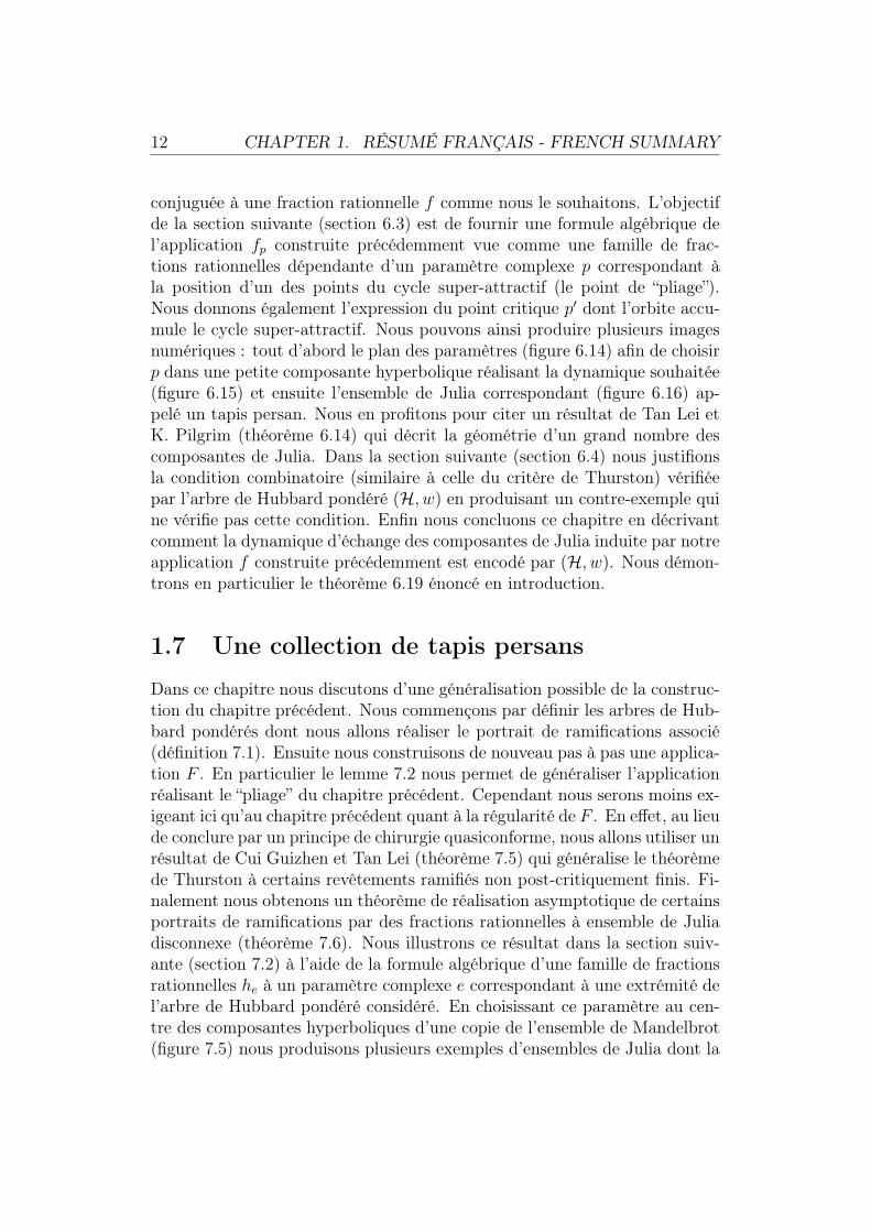
conjuguée à une fraction rationnelle f comme nous le souhaitons. L’objectifde la section suivante (section 6.3) est de fournir une formule algébrique del’application fp construite précédemment vue comme une famille de frac-tions rationnelles dépendante d’un paramètre complexe p correspondant àla position d’un des points du cycle super-attractif (le point de “pliage”).Nous donnons également l’expression du point critique p′ dont l’orbite accu-mule le cycle super-attractif. Nous pouvons ainsi produire plusieurs imagesnumériques : tout d’abord le plan des paramètres (figure 6.14) afin de choisirp dans une petite composante hyperbolique réalisant la dynamique souhaitée(figure 6.15) et ensuite l’ensemble de Julia correspondant (figure 6.16) ap-pelé un tapis persan. Nous en profitons pour citer un résultat de Tan Lei etK. Pilgrim (théorème 6.14) qui décrit la géométrie d’un grand nombre descomposantes de Julia. Dans la section suivante (section 6.4) nous justifionsla condition combinatoire (similaire à celle du critère de Thurston) vérifiéepar l’arbre de Hubbard pondéré (H, w) en produisant un contre-exemple quine vérifie pas cette condition. Enfin nous concluons ce chapitre en décrivantcomment la dynamique d’échange des composantes de Julia induite par notreapplication f construite précédemment est encodé par (H, w). Nous démon-trons en particulier le théorème 6.19 énoncé en introduction.
1.7 Une collection de tapis persans
Dans ce chapitre nous discutons d’une généralisation possible de la construc-tion du chapitre précédent. Nous commençons par définir les arbres de Hub-bard pondérés dont nous allons réaliser le portrait de ramifications associé(définition 7.1). Ensuite nous construisons de nouveau pas à pas une applica-tion F . En particulier le lemme 7.2 nous permet de généraliser l’applicationréalisant le “pliage” du chapitre précédent. Cependant nous serons moins ex-igeant ici qu’au chapitre précédent quant à la régularité de F . En effet, au lieude conclure par un principe de chirurgie quasiconforme, nous allons utiliser unrésultat de Cui Guizhen et Tan Lei (théorème 7.5) qui généralise le théorèmede Thurston à certains revêtements ramifiés non post-critiquement finis. Fi-nalement nous obtenons un théorème de réalisation asymptotique de certainsportraits de ramifications par des fractions rationnelles à ensemble de Juliadisconnexe (théorème 7.6). Nous illustrons ce résultat dans la section suiv-ante (section 7.2) à l’aide de la formule algébrique d’une famille de fractionsrationnelles he à un paramètre complexe e correspondant à une extrémité del’arbre de Hubbard pondéré considéré. En choisissant ce paramètre au cen-tre des composantes hyperboliques d’une copie de l’ensemble de Mandelbrot(figure 7.5) nous produisons plusieurs exemples d’ensembles de Julia dont la

CHAPTER 1. RÉSUMÉ FRANÇAIS - FRENCH SUMMARY 13
dynamique d’échange des composante est encodée par des arbres pondérés(figure 7.4, figure 7.6 et figure 7.7). Le choix d’un paramètre correspondantà un point de Misiurewicz de la copie de l’ensemble de Mandelbrot permetmême d’obtenir d’autres exemples qui ne sont pas couverts par notre résultat(figure 7.8).
1.8 ConclusionFinalement nous concluons cette thèse par quelques questions soulevées parces travaux et par des projets futurs. Tout d’abord nous envisageons unraffinement du théorème 6.18 afin d’étendre continuement la conjugaison surles composantes de Julia à toute la sphère de Riemann. Nous proposons uneméthode à l’aide du résultat de Cui Guizhen et Tan Lei (théorème 7.5) discutéau chapitre précédent. Cette méthode permet aussi d’espérer un encodagepour les applications produites par le théorème 7.6. Ensuite nous discutonsd’une généralisation possible de la construction du chapitre précédent à desarbres de Hubbard pondérés plus généraux que ceux de la définition 7.1.Enfin nous soulevons des questions à plus long terme à propos de l’unicité(à conjugaison quasiconforme près) de fractions rationnelles encodées par unmême arbre de Hubbard pondéré et également à propos du problème inverse,à savoir déduire la structure d’arbre derrière la dynamique d’échange descomposantes de Julia d’une fraction rationnelle donnée.
Chapter 2
Introduction
Let C be the Riemann sphere. We will use S2 when we wish to think topo-logically (that is the one-point compactification of the complex plane C) andC when we wish to think analytically (emphasizing the complex structureas one-dimensional complex manifold). Recall that the set of holomorphicmaps on C is equal to the set of rational maps, that is the set of ratios ofpolynomials with complex coefficients.
Let f : C → C be a rational map. The aim of holomorphic dynamicalsystems theory is to study the forward orbit under iterations by f of everystarting point z0 ∈ C:
z0f7→ z1
f7→ z2f7→ z3
f7→ . . .
To do so, the Riemann sphere is divided in two sets of starting points whichlead to two different kinds of behavior. These sets are named after two math-ematicians whose works flowered the global study of holomorphic dynamicalsystems during the early 20th century.
Definition 2.1 (Fatou and Julia sets). Let f : C → C be a rational map.The Fatou set of f , denoted by F(f), is the domain of normality for thecollection of iterates f n / n > 1, that is the set of z ∈ C which admits aneighbourhood Vz ⊂ C such that the sequence (f n|Vz)n>1 of holomorphic mapshas subsequence which converges uniformly on compact subsets of Vz. TheJulia set of f , denoted by J (f), is the complement in C of the Fatou set.
J (f) = C−F(f)
Many authors present the basics to study the geometrical and dynamicalproperties of those two sets, see in particular [Bea91], [CG93], [BM01] or[Mil06]. We would like here to focus on some results which motivate thisthesis.

CHAPTER 2. INTRODUCTION 15
Theorem 2.2. For any rational map f : C → C of degree two or more,the Julia set J (f) is a nonempty fully invariant compact set without isolatedpoint. Furthermore
• either J (f) is connected,
• or else J (f) has uncountably many connected components.
Figure 2.1 illustrates this dichotomy.
Figure 2.1: Two Julia sets of quadratic polynomials:one connected called the Douady’s rabbit
and one totally disconnected
We are going to discuss the second case and particularly the exchangingdynamics of Julia components (that is the induced dynamical system on theset of every connected components of the Julia set).
In this way, we are going to state at first a classical result (see [Bea91]).Recall that a fixed point z0 ∈ C of a rational map f : C → C is saidattracting if it satisfies |f ′(z0)| < 1 (or | limz→∞
1f ′(z)| < 1 if z0 = ∞). In
that case we define the immediate attracting bassin of z0 to be the connectedcomponent containing z0 of the set of points whose forward orbits accumulatez0. Recall also that a Cantor set is a nonempty compact set which is perfect(without isolated point) and totally disconnected (each connected componentis a single point). For instance the second Julia set in Figure 2.1 is a Cantorset (actually it is a consequence of the following result).

16 CHAPTER 2. INTRODUCTION
Theorem 2.3. Let f : C → C be a rational map of degree d > 2. Ifthere exists an attracting fixed point z0 of f such that every critical point off lies in the immediate attracting bassin of z0 then J (f) is a Cantor set.More precisely there exists a homeomorphism ϕ : J (f) → Σd such that thefollowing diagram commutes
J (f)f //
ϕ
J (f)
ϕ
Σd σ// Σd
where
• Σd = 1, 2, . . . , dN is a Cantor set for the metric
∀ε, ε′ ∈ Σd, dΣd(ε, ε′) =
+∞∑i=0
|εi − ε′i|(d+ 1)i
• σ : Σd → Σd is the shift map that is ∀ε ∈ Σd, σ(ε0ε1ε2 . . . ) = ε1ε2ε3 . . .
Notice that the assumption is satisfied for quadratic polynomials of theform z 7→ z2 + c with a sufficiently large value of c (like the second Julia setin Figure 2.1).
This result allows to understand the entire exchanging dynamics of Juliacomponents in that case. For instance, if follows easily that the periodicpoints are dense in the Julia set or that there is a dense set of points in theJulia set whose forward orbits are dense in the Julia set.
We would like to obtain a similar result for Julia sets with more compli-cated components than single points. Unfortunatly we do not know severalexamples of such Julia sets. Indeed B. Branner and J. H. Hubbard provedin [BH92] that in polynomial case, all but countably many Julia componentsmust be single points. This is certainly not true for arbitrary rational mapsbut we will see later (see Theorem 6.14) that Tan Lei and K. Pilgrim provedin [PT00] that under a certain condition, all but countably many Julia com-ponents must be either a point or a Jordan curve.
The example in Figure 2.2, due to C. T. McMullen, has uncountablymany connected components which are Jordan curves (see [Bea91] or [Mil06]).Roughly speaking, this Julia set is a Cantor set of circles (denoted by “CoC”in shorter) that is like the set
⋃r∈Cz ∈ C / |z| = r where C is some Cantor
set on the positive real line.Actually we can describe the entire exchanging dynamics of Julia com-
ponents for this example (see [Bea91]). We denote by fCoC the rational map

CHAPTER 2. INTRODUCTION 17
Figure 2.2: Example of Julia set which is a Cantor set of circles
whose Julia set is drawn in Figure 2.2 and by JCoC the set of Julia com-ponents equipped with the Hausdorff topology coming from the followingHausdorff metric:
∀J, J ′ ∈ JCoC, dH(J, J ′) = max
supz∈J
infz′∈J ′|z − z′|, sup
z′∈J ′infz∈J|z − z′|
Then fCoC induces on JCoC a continuous dynamical system denoted also byfCoC : JCoC → JCoC.
Proposition 2.4. There exists a homeomorphism φ : JCoC → Σ2 such thatthe following diagram commutes
JCoCfCoC //
φ
JCoC
φ
Σ2 σ// Σ2
Recall that the Cantor ternary set Σ2 may be seen as the non-escapingset of a continuous dynamical system on the unit segment [0, 1]:
τC : [0, 1] → [0, 1]
x 7→
3x if x ∈ [0, 12]
3(1− x) if x ∈ [12, 1]

18 CHAPTER 2. INTRODUCTION
Σ2 is homeomorphic to the following non-escaping set
JC =
x ∈ [0, 1] /∀n > 0, τ nC (x) ∈
[0,
1
3
]∪[
2
3, 1
]We may thus reformulate Proposition 2.4 as follows:
Proposition 2.5. There exists a homeomorphism ϕ : JCoC → JC such thatthe following diagram commutes
JCoCfCoC //
ϕ
JCoC
ϕ
JC τC// JC
Any Julia component J ∈ JCoC, that is any any preimage by ϕ of a point inJC, is a Jordan curve.
Figure 2.3: A “thickening” of JC ⊂ [0, 1] → R3
(compare with Figure 2.2)
Heuristically speaking, we may think of the action of fCoC as that one ofτC on the boundary (homeomorphic to the sphere S2) of a small “thickening”of the unit segment [0, 1] embedded in R3 as it is suggested in Figure 2.3.Indeed fCoC is of the form z 7→ z2 + λ/z3 where λ is sufficiently small and astudy of Fatou components (see [Bea91]) shows that the immediate attractingbassin F∞ of ∞ is simply connected (that corresponds to a neighbourhoodof 0 for τC), the preimage F0 of F∞ contains the other critical points and isalso simply connected (that corresponds to a neighbourhood of 1 for τC) andall other Fatou components are doubly connected.
In this thesis, we would like to construct some other examples of rationalmaps with complicated Julia sets and whose dynamics is encoded by somecombinatorial data. To do so, we will discuss the construction of rationalmaps with prescribed dynamics. The two main tools in this discussion willbe the quasiconformal surgery method and the Thurston’s characterizationof post-critically finite rational maps.

CHAPTER 2. INTRODUCTION 19
In particular, we will get the following concrete example (see Chapter 6).
Theorem 2.6. There exists a rational map f : C → C whose Julia set isdrawn in Figure 2.4 and a homeomorphism ϕ from a subset JH(f) of Juliacomponents of f equipped with a certain topology such that the followingdiagram commutes
JH(f)f //
ϕ
JH(f)
ϕ
JHPc
// JH
where JH is a Cantor set which is the intersection between the Julia set ofa quadratic polynomial Pc : z 7→ z2 + c (actually c ≈-0.157+1.032i) and theassociated Hubbard tree (see Example 6.6).
Moreover there exists only one fixed Julia component in JH(f) denotedby Jα (which is quasiconformally mapped onto the connected Julia set of another rational map) and any Julia component J ∈ JH(f) which is not mappedafter some iterations of f onto Jα is a Jordan curve.
Figure 2.4: A disconnected Julia set
In particular that proves there are some Julia components of f whichdoes not meet the boundary of any Fatou components (for instance Jα andall of their preimages).

Chapter 3
Prescribed dynamics
We are going to give some meanings behind what is prescribed dynamics.The aim is to impose the action of a rational map, or more generally of aramified covering, on its critical and post-critical sets. To do so, we willintroduce the ramification portraits and some related definitions (following[Koc07] and according to works in [BFH92]). Then we will begin to discussthe question of finding rational maps of prescribed dynamics. The arisingproblems should lead to the two next chapters.
3.1 Ramification portraits
We first establish some standard notations and definitions. To each ramifiedcovering f : S2 → S2 we denote by Ωf = critical points of f its critical setand by Pf =
⋃n>1 f
n(Ωf ) its post-critical set. The action of f on Ωf ∪ Pfis totally encoded by the surjective restriction σf = f|Ωf∪Pf : Ωf ∪ Pf → Pfand the local degree νf = degloc(f)|Ωf∪Pf : Ωf ∪ Pf → N − 0. That leadsto the following definition (according to [Koc07]).
Definition 3.1 (ramification portrait). A ramification portrait is the dataof
• a finite set Ω ⊂ S2
• a set (not necessarily finite or disjoint from Ω) P ⊂ S2
• a surjective map σ : Ω ∪ P → P
• a function ν : Ω ∪ P → N− 0 such that ν−1 (n ∈ N/n > 2) = Ω
We denote by R = (Ω, P, σ, ν) such a ramification portrait.

CHAPTER 3. PRESCRIBED DYNAMICS 21
Remark that the critical set of a ramified covering f : S2 → S2 is wellfinite since the critical points of f are isolated points of the compact set S2.In particular, f is of finite degree deg(f) and it has exactly 2 deg(f) − 2critical points, counted with multiplicity, by the Riemann-Hurwitz formula(see Theorem A.12 in appendix).
Definition 3.2 (degree of a ramification portrait). The degree of a ramifi-cation portrait R = (Ω, P, σ, ν), denoted by deg(R), is the number
deg(R) = 1 +1
2
∑ω∈Ω
(ν(ω)− 1)
Obviously we have:
Proposition 3.3. If f is a ramified covering of critical set Ωf and post-critical set Pf then (Ωf , Pf , σf = f|Ωf∪Pf , νf = degloc(f)|Ωf∪Pf ) is a ramifica-tion portrait and deg(Rf ) is equal to the degree deg(f) of f .
Definition 3.4 (ramification portrait of a ramified covering). We denoteby Rf = (Ωf , Pf , σf = f|Ωf∪Pf
, νf = degloc(f)|Ωf∪Pf) the ramification
portrait associated to a ramified covering f : S2 → S2. In case f : C → Cwould be a rational map, we identify S2 with C as topological manifolds inorder to define the associated ramification portrait of f as well.
Notice that the degree of a ramification portrait R = (Ω, P, σ, ν) is notnecessarily an integer, indeed deg(R) ∈ 1
2Z. Moreover the number of preim-
ages by σ of a point in P may be larger than the degree deg(R). So we willrestrict our discussion to a special subset of ramification portraits definedbelow.
Definition 3.5 (branch compatible ramification portrait). A ramificationportrait R = (Ω, P, σ, ν) is said branch compatible if
∀ω ∈ P,∑
x∈Ω∪Pσ(x)=ω
ν(x) 6 deg(R)
Definition 3.6 (ramification portrait of polynomial type). R = (Ω, P, σ, ν)is a ramification portrait of polynomial type if
(i) R is branch compatible
(ii) ∃ω ∈ Ω ∪ P/σ(ω) = ω and ν(ω) = deg(R)
22 CHAPTER 3. PRESCRIBED DYNAMICS
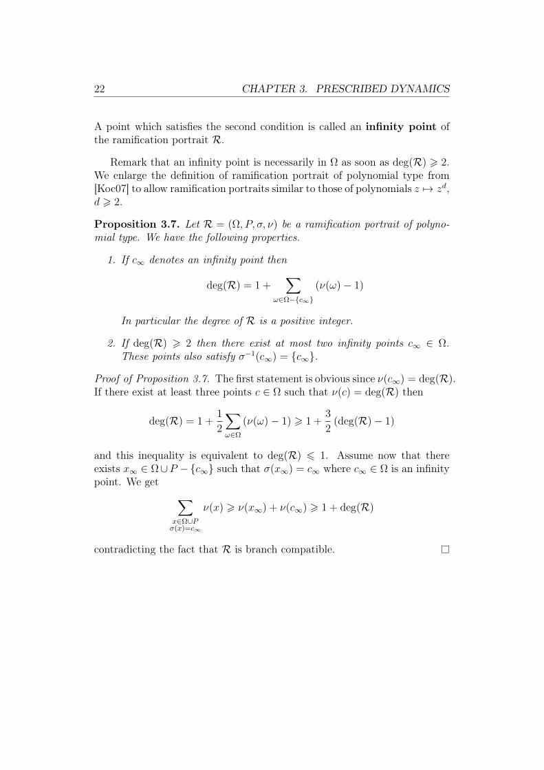
A point which satisfies the second condition is called an infinity point ofthe ramification portrait R.
Remark that an infinity point is necessarily in Ω as soon as deg(R) > 2.We enlarge the definition of ramification portrait of polynomial type from[Koc07] to allow ramification portraits similar to those of polynomials z 7→ zd,d > 2.
Proposition 3.7. Let R = (Ω, P, σ, ν) be a ramification portrait of polyno-mial type. We have the following properties.
1. If c∞ denotes an infinity point then
deg(R) = 1 +∑
ω∈Ω−c∞
(ν(ω)− 1)
In particular the degree of R is a positive integer.
2. If deg(R) > 2 then there exist at most two infinity points c∞ ∈ Ω.These points also satisfy σ−1(c∞) = c∞.
Proof of Proposition 3.7. The first statement is obvious since ν(c∞) = deg(R).If there exist at least three points c ∈ Ω such that ν(c) = deg(R) then
deg(R) = 1 +1
2
∑ω∈Ω
(ν(ω)− 1) > 1 +3
2(deg(R)− 1)
and this inequality is equivalent to deg(R) 6 1. Assume now that thereexists x∞ ∈ Ω∪P −c∞ such that σ(x∞) = c∞ where c∞ ∈ Ω is an infinitypoint. We get ∑
x∈Ω∪Pσ(x)=c∞
ν(x) > ν(x∞) + ν(c∞) > 1 + deg(R)
contradicting the fact that R is branch compatible.
CHAPTER 3. PRESCRIBED DYNAMICS 23
3.2 Realization
Example 3.8. LetR be a ramification portrait of polynomial type displayedbelow.
c02 // c1
1 // c2 1gg c∞ 2jj
In this example, Ω = c0, c∞ and P = c1, c2, c∞. The arrows above depictthe map σ : Ω ∪ P → P . To each ω ∈ Ω ∪ P the integer ν(ω) is assigned tothe arrow leaving from ω: ν(c0) = ν(c∞) = 2 and ν(c1) = ν(c2) = 1.
To find a polynomial f (f acts on C but we identify C to S2) such thatRf = R implies at first that deg(f) = deg(R) = 2 and c∞ = ∞. Hencef is a quadratic polynomial. From the informations f ′(c0) = 0, f(c0) = c1
and f(c1) = c2 we get that the form of f is f(z) = (c2−c1)(c1−c0)2
(z − c0)2 + c1.The last information f(c2) = c2 gives an algebraic relation linking c0, c1
and c2 that is c0 = c1+c22
. Finally there exists a polynomial of associatedramification portrait R if and only if c∞ = ∞ and c0 = c1+c2
2. For instance
we get z 7→ z2 − 2 for c0 = 0, c1 = −2 and c2 = 2.
As it is shown in the example above, to find a polynomial of given associ-ated ramification portrait may be not possible. Fixing the position of criticaland post-critical points on the sphere S2 is too restrictive.
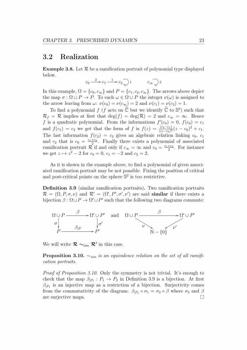
Definition 3.9 (similar ramification portraits). Two ramification portraitsR = (Ω, P, σ, ν) and R′ = (Ω′, P ′, σ′, ν ′) are said similar if there exists abijection β : Ω∪P → Ω′∪P ′ such that the following two diagrams commute:
Ω ∪ Pβ //
σ
Ω′ ∪ P ′
σ′
Pβ|P // P ′
and Ω ∪ Pβ //
ν %%
Ω′ ∪ P ′
ν ′xxN− 0
We will write R ∼sim R′ in this case.
Proposition 3.10. ∼sim is an equivalence relation on the set of all ramifi-cation portraits.
Proof of Proposition 3.10. Only the symmetry is not trivial. It’s enough tocheck that the map β|P1 : P1 → P2 in Definition 3.9 is a bijection. At firstβ|P1 is an injective map as a restriction of a bijection. Surjectivity comesfrom the commutativity of the diagram: β|P1 σ1 = σ2 β where σ2 and βare surjective maps.

24 CHAPTER 3. PRESCRIBED DYNAMICS
Definition 3.11 (realization of a ramification portrait). We say that a ram-ified covering f : S2 → S2 (or a rational map f : C → C) realizes aramification portrait R if Rf ∼sim R.
For instance, the polynomial z 7→ z2−2 realizes the ramification portraitof Example 3.8 for any choice of points c0, c1, c2 and c∞ on S2.
So we may consider a prescribed dynamics as an equivalence class of∼sim. That does not provide a combinatorial tool which captures the wholedynamical information about a ramified covering and we will discuss latersome attempts to make the meaning behind prescribed dynamics sharper.But for the moment, to find a rational map with prescribed dynamics meansto realize a ramification portrait by a rational map.
However we will need a less restrictive definition in case of infinite rami-fication portrait in order to deal with only a finite number of informations.
Definition 3.12 (asymptotic realization). Let f : S2 → S2 be a ramifiedcovering (or more generally let f : C → C be a rational map). We denoteby Ω′f the set of critical points with finite forward orbit under iteration of fand by R′f the induced ramification portrait:
• Ω′f = ω ∈ Ωf / |⋃n>1 f
n(ω)| <∞
• R′f = (Ω′f , P′f =
⋃n>1 f
n(Ω′f ), σ′f = f|Ω′f∪P ′f , ν
′f = degloc(f)|Ω′f∪P ′f )
Then we say that f realizes asymptotically a finite ramification portraitR if the following conditions hold:
(i) R′f ∼sim R
(ii) the accumulation set of the post-critical set of f is contained in Ω′f∪P ′f ,in other words the orbit
⋃n>1 f
n(ω) of every critical point ω ∈ Ωf−Ω′faccumulates a periodic cycle in Ω′f ∪ P ′f
Example 3.13. Consider a quadratic polynomial Pc of the form z 7→ z2 +c with a sufficiently large value of c. Then Pc realizes asymptotically theramification portrait below
∞ 2gg 0 2 // c
where the waved arrow means that the critical point 0 is mapped in theimmediate attracting bassin of ∞.

CHAPTER 3. PRESCRIBED DYNAMICS 25
3.3 Examples
Unfortunately not every ramification portrait can be realized by rationalmaps. We will see two examples of such ramification portraits which arecharacteristic of the two kinds of problems (or obstructions) that could arise.
Example 3.14 (Topological obstruction). Let Rtop be the ramification por-trait below.
c02 // c1
1 ))c2
1
ii c∞ 2jj
If a rational map realizes this ramification portrait, this map would be ofdegree deg(Rtop) = 2. But there are at least three preimages of c1, countedwith multiplicity (c2 of multiplicity 1 and c0 of multiplicity 2), which isimpossible for a map of degree two. In fact Rtop is not branch compatible.
Indeed the Riemann-Hurwitz formula (see Theorem A.12 in appendix)provides many restrictions on the ramification portrait of a ramified covering.If a ramification portrait violates these restrictions, it cannot be realized byany ramified covering (and in particular by any rational map). Consequentlyour first objective will be to discuss the realization of ramification portraitsby ramified coverings (that is a purely topological discussion).
Example 3.15 (Analytical obstruction). Let Rana be the ramification por-trait of polynomial type below.
c02 // c1
1 ))c2
1
ii c∞ 3jj
c′21
55 c′11uu
c′02oo
This example seems to have no topological obstruction as the previous exam-ple. Each point of the post-critical set has less than three preimages, countedwith multiplicity, and deg(Rana) = 3. Indeed we will see in the next chapterthat Rana can be realized by a ramified covering fana. For the moment, iden-tifying S2 − c∞ with the complex plane C and assuming that the criticaland post-critical sets belong to the real line R, we can at least construct therestriction fana|R on the real axis (see Figure 3.1): c0 and c′0 are the onlypoints where fana|R is not locally injective (the “critical points”), even wherefana|R is locally two-to-one (of “local degree two”) and the action of fana|R onthe forward orbits of c0 and c′0 is the same, up to composition by a bijection,as the one of σana.

26 CHAPTER 3. PRESCRIBED DYNAMICS
Figure 3.1: A continuous and piecewise affine map fana|R which realizes Rana
But we will see (in Chapter 5) that fana cannot be “perturbed” in orderto get a polynomial! In that case the obstruction is not topological (sinceRana can be realized by a ramified covering) but it comes from the analyticalstructure we equip the sphere S2 with. Therefore our second objective willbe to discuss the realization by some rational maps of ramification portraitsalready realized by some ramified coverings. We will forget the topologicalobstructions to concentrate on the analytical part of the problem.


Chapter 4
Topological trees
In this chapter, we would like to concentrate on the realization of finiteramification portraits by some ramified coverings. To do so, we introducedynamical trees and some related definitions (following [Poi93]) to be alsouseful for discussions coming later (Chapter 6). Then we will construct ram-ified coverings realizing some particular ramification portraits and we willdiscuss the general case with an example.
4.1 Dynamical trees
Definition 4.1 (planar tree). A planar tree is a finite connected acyclicplanar graph T = (V,E), that is the data of
• a finite set V ⊂ C of vertices
• a finite set E of pairwise disjoint (except possibly at the ends) Jor-dan arcs ev1,v2 , called edges, between some unordered pairs of distinctvertices v1, v2 ∈ V
such that for any pair of distinct vertices v, v′ ∈ V there exists a uniqueJordan arc linking v and v′ as the union of distinct edges:
[v, v′]T = ev0=v,v1 ∪ ev1,v2 ∪ · · · ∪ evn−1,vn=v′
We will not distinguish between the tree T and its planar pattern⋃e∈E e ⊂ C.
More precisely planar graph in definition above means a simplicial com-plex of dimension 1 embedded in the complex plane, and it is a planar treeif its complement in the complex plane is connected.

CHAPTER 4. TOPOLOGICAL TREES 29
Definition 4.2 (valency). For every vertex v ∈ V of a planar tree T = (V,E),let Ev⊂ E be the set of edges of T with v as a common endpoint. We callvalency the number of edges in Ev which is equal to the number of connectedcomponents of T − v. We say that v is a branching point if |Ev| > 2 andan end if |Ev| = 1.
Remark that every Ev comes with a cyclic order induced by the usualcounterclockwise orientation on C.
For any integer n ∈ N, denote by Un the cyclicly ordered group of nth
roots of unity.
Definition 4.3 (dynamical tree). A dynamical tree is the data of
• an underlying planar tree T = (V,E)
• a map of vertices dynamics τ : V → V
• a local degree function δ : V → N− 0
such that
(i) For any edge ev,v′ ∈ E with endpoints v, v′ ∈ V , the two imagesτ(v), τ(v′) ∈ V must be distinct.
The assumption above allows us to extend τ continuously to T as follows: forany edge ev,v′ ∈ E with endpoints v, v′ ∈ V , define τ : ev,v′ → [τ(v), τ(v′)]Tto be a homeomorphism where [τ(v), τ(v′)]T is the unique Jordan arc in Tlinking τ(v) to τ(v′). This extension of τ induces naturally a well definedmap τv : Ev → Eτ(v) for any vertex v ∈ V .
(ii) For any vertex v ∈ V , there exist an order preserving bijection βv :Eτ(v) → Un, where n = |Eτ(v)| is the valency of τ(v), together with anorder preserving injection ιv : Ev → Uδ(v)n where δ(v) is the assigneddegree at v, such that the following diagram commutes
Ev ιv //
τv
Uδ(v)n
e2iπθ 7→ e2iπδ(v)θ
Eτ(v)
βv
∼ // Un
We denote by T = (T, τ, δ) such a dynamical tree.

30 CHAPTER 4. TOPOLOGICAL TREES
Figure 4.1 shows an example illustrating the second condition. One wayto interpret this condition is that we lift by z 7→ zδ(v) a star of n edges to geta star of δ(v)n edges, and our map τ near v should behave like z 7→ zδ(v) ona sub-star of the lifted star. This condition implies in particular
∀v ∈ V, |Ev| 6 δ(v)|Eτ(v)|
Figure 4.1: Example of vertex in dynamical tree with local degree 4
Definition 4.4 (critical and post-critical points of a dynamical tree). Wesay that a vertex v ∈ V of a dynamical tree T = (T, τ, δ) is a criticalpoint if δ(v) > 2 and a post-critical point if there exist an integer n > 1and a critical point w ∈ V such that v = τ n(w). We denote by ΩT =critical points of T the critical set of T and by PT =
⋃n>1 τ
n(ΩT ) thepost-critical set.
Definition 4.5 (degree of a dynamical tree). The degree of a dynamicaltree T = (T, τ, δ), denoted by deg(T ), is the number
deg(T ) = 1 +∑v∈V
(δ(v)− 1)

CHAPTER 4. TOPOLOGICAL TREES 31
Definition 4.6 (extension of a dynamical tree). Let T = (T, τ, δ) and T =
(T , τ , δ) be two dynamical trees of same degree deg(T ) = deg(T ). We say
that T is an extension of T if there exists an injective map φ :
V → V
E → E
such that
(i) the following two diagrams commute
Vφ //
τ
V
τV
φ// V
and Vφ //
δ ##
V
δN− 0
(ii) for any vertex v ∈ V , φ induces a cyclic order preserving injection ofEv into Eφ(v)
We will write T T in this case.
To obtain T from T we may add extra non-critical vertices on the edgesof T and/or extra edges linking vertices of T to extra non-critical verticesoutside of T . Obviously we have:
Proposition 4.7. is a partial order relation on the set of all dynamicaltrees.
Therefore the following definition determines an equivalence relation.
Definition 4.8 (equivalent dynamical trees). Two dynamical trees T =(T, τ, δ) and T ′ = (T ′, τ ′, δ′) of same degree are said equivalent if T T ′and T ′ T . We will write T ' T ′ in this case.
4.2 Stars and surgeryWe would like to prove that we may extend (using “topological surgery”)some dynamical trees to the whole complex plane C by ramified coverings inorder to realize some particular ramification portraits of polynomial type.
Definition 4.9 (N -cyclic ramification portrait of polynomial type). LetR =(Ω, P, σ, ν) be a ramification portrait of polynomial type and c∞ be an infinitypoint. R is said N -cyclic for a positive integer N if every critical pointω ∈ Ω− c∞ is periodic under iteration of σ (i.e. Ω ⊂ P ) and P − c∞ isthe union of exactly N disjoint periodic cycles.
32 CHAPTER 4. TOPOLOGICAL TREES
Remark that this definition does not depend on the choice of infinitypoint in case there exist two of them. Moreover if a ramification portrait ofpolynomial type R is N -cyclic for a positive integer N then deg(R) > 2.
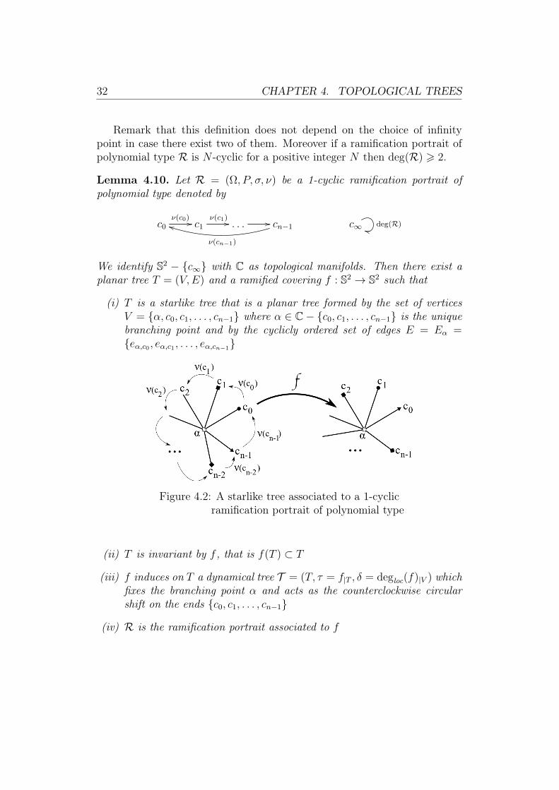
Lemma 4.10. Let R = (Ω, P, σ, ν) be a 1-cyclic ramification portrait ofpolynomial type denoted by
c0ν(c0) // c1
ν(c1) // . . . // cn−1
ν(cn−1)
jj c∞ deg(R)jj
We identify S2 − c∞ with C as topological manifolds. Then there exist aplanar tree T = (V,E) and a ramified covering f : S2 → S2 such that
(i) T is a starlike tree that is a planar tree formed by the set of verticesV = α, c0, c1, . . . , cn−1 where α ∈ C− c0, c1, . . . , cn−1 is the uniquebranching point and by the cyclicly ordered set of edges E = Eα =eα,c0 , eα,c1 , . . . , eα,cn−1
Figure 4.2: A starlike tree associated to a 1-cyclicramification portrait of polynomial type
(ii) T is invariant by f , that is f(T ) ⊂ T
(iii) f induces on T a dynamical tree T = (T, τ = f|T , δ = degloc(f)|V ) whichfixes the branching point α and acts as the counterclockwise circularshift on the ends c0, c1, . . . , cn−1
(iv) R is the ramification portrait associated to f

CHAPTER 4. TOPOLOGICAL TREES 33
Proof of Lemma 4.10. From the fact that the complex plane minus a finitenumber of points is arcwise connected, we can easily find a planar tree T =(V,E) which satisfies the condition (i) for any choice of branching pointα ∈ C−c0, c1, . . . , cn−1. It is also possible to construct carefully the edgesof T in such a way they are locally connected. Let τ : V → V be themap which fixes the branching point α and acts as the counterclockwisecircular shift on the ends c0, c1, . . . , cn−1. Extend continuously this mapto T as in Definition 4.3 and denote by τ = f|T this extension. Remarkthat any extension of f|T to S2 satisfies the condition (ii). Recall that ifR = (Ω, P, σ, ν) is the ramification portrait associated to such an extensionf (as in condition (iv)), then degloc(f)|V = ν (with the extra definitionν(α) = 1). Moreover T = (T, τ = f|T , δ = ν) is a well defined dynamical treeas in condition (iii). Therefore it is sufficient to prove that f|T extends to S2
as a ramified covering f whose associated ramification portrait is R.Now consider the extension T = (T , τ , δ) of T as follows (see Figure 4.3)
Figure 4.3: The extension T in proof of Lemma 4.10
• for each end ck where k ∈ 0, 1, . . . , n − 1, add ν(ck) − 1 extra edgeslinking ck to extra vertices denoted by α1
k, α2k, . . . , α
ν(ck)−1k such that
Eck = eck,α, eck,α1k, eck,α2
k, . . . , e
ck,αν(ck)−1
k
is cyclicly ordered
• for each vertex αjk where j ∈ 1, 2, . . . , ν(ck)−1, add n−1 extra edgeslinking αjk to extra vertices denoted by cjk,0, . . . , c
jk,k−1, c
jk,k+1, . . . , c
jk,n−1
such that Eαjk = eαjk,cjk,0 , . . . , eαjk,cjk,k−1, eαjk,c
jk,k+1
, . . . , eαjk,cjk,n−1 is cyclicly
ordered

34 CHAPTER 4. TOPOLOGICAL TREES
• define τ : V → V as followsτ(α) = ατ(ck) = ck+1 where k ∈ 0, 1, . . . , n− 1τ(αjk) = α where k ∈ 0, 1, . . . , n− 1, j ∈ 1, 2, . . . , ν(ck)− 1τ(cjk,`) = c`+1 where k 6= ` ∈ 0, 1, . . . , n− 1, j ∈ 1, 2, . . . , ν(ck)− 1
with the notation cn = c0
• extend continuously τ to T by τ on T and by homeomorphisms onevery extra edge
Remark that we may construct carefully each extra edge in such a way theyare locally connected. Remark also that τ(T ) = T and the valency of eachck where k ∈ 0, 1, . . . , n− 1 is now δ(ck) = ν(ck) in T . Therefore
∀k ∈ 0, 1, . . . , n− 1, |Eck | = ν(ck)|Eτ(ck)| (4.1)
Consider T and its image τ(T ) = T as if they belong to two differentcopies of S2 (recall that we identify C with S2 − c∞), say respectively S1
and S2 (see Figure 4.4). We are going to construct a ramified covering fwhich extends continuously τ by surgery.
Since T is simply connected, we may easily define a cyclicly ordered setA2 of |A2| = n disjoint (except at c∞) Jordan arcs in S2 − T (except at ck)linking c∞ to each ck where k ∈ 0, 1, . . . , n− 1 (see Figure 4.4).
Since T is connected, Riemann’s mapping theorem provides a biholo-morphic map ϕ1 : D → S1 − T such that ϕ1(0) = c∞. Moreover we haveconstructed T to be locally connected. By Carathéodory’s theorem we maythus extend continuously ϕ1 to D. Remark that
• each end cjk,` where k 6= ` ∈ 0, 1, . . . , n−1 and j ∈ 1, 2, . . . , ν(ck)−1has exactly one preimage in ∂D by ϕ1
• each branching point ck where k ∈ 0, 1, . . . , n − 1 has exactly ν(ck)preimages in ∂D by ϕ1 (since ν(ck) corresponds to the valency of ck)
Then define a cyclic ordered set A1 of Jordan arcs (see Figure 4.4) as im-ages by ϕ1 of straight rays in D linking 0 to those preimages in ∂D. Using

CHAPTER 4. TOPOLOGICAL TREES 35
Figure 4.4: The piecewise definition of the ramifiedcovering f in Lemma 4.10
Proposition 3.7, we get:
|A1| = (n− 1)n−1∑k=0
(ν(ck)− 1) +n−1∑k=0
ν(ck)
= nn−1∑k=0
(ν(ck)− 1) + n
= n(deg(R)− 1) + n
= deg(R)|A2| (4.2)
Now define f|T∪A1: T ∪ A1 → T ∪ A2 to be equal to τ on T and and to
be continuously extended to each Jordan arc in A1 linking a ∈ T to c∞ by

36 CHAPTER 4. TOPOLOGICAL TREES
homeomorphism onto the Jordan arc in A2 linking τ(a) to c∞. It remainsdeg(R) × n connected components of S1 − (T ∪ A1) which are topologicaldisks whose boundaries are Jordan curves formed by the union of exactly twoedges of T and two Jordan arcs in A1 (see Figure 4.4). Remark that f|T∪A1
is defined as a homeomorphism on each of those Jordan curves. Thereforewe may extend homeomorphically f|T∪A1
to every connected component ofS1 − (T ∪ A1) onto a connected component of S2 − (T ∪ A2) by Schönflies’theorem (see Theorem A.3 in appendix). Finally the equalities (4.1) and (4.2)together with the cyclic orders on A1, A2 and Eck for every k ∈ 0, 1, . . . , n−1 ensure that we get a ramified covering f : (S1 = S2) → (S2 = S2) whoseassociated ramification portrait is R as required.
Before doing as well for any N -cyclic ramification portrait of polynomialtype, we need the following sharpening.
Lemma 4.11. Use notations from Lemma 4.10 and assume in addition thatc0 is a critical point. Then we can find a planar tree T = (V,E) and aramified covering f : S2 → S2 which satisfy conditions (i), (ii), (iii), (iv)together with
(v) there exists an extension T ′ = (T ′, τ ′ = f|T ′ , δ′ = degloc(f)|V ′) of T
which consists in adding one extra vertex β ∈ C − α, c0, c1, . . . , cn−1and one extra edge ec0,β such that f(β) = β and f(ec0,β) ⊂ T ′
Notice that with a suitable indexing of points in Ω ∪ P , we may alwaysassume that c0 is a critical point. The condition (v) implies in particular (seeFigure 4.5)
f(ec0,β) = [c1, β]T ′ = ec1,α ∪ eα,c0 ∪ ec0,β
Figure 4.5: The beta point

CHAPTER 4. TOPOLOGICAL TREES 37
Proof of Lemma 4.11. Let us come back to the proof of Lemma 4.10. Denoteby D1 the connected component of S1 − (T ∪A1) whose boundary is formedby the union of two edges of T and two Jordan arcs in A1 linking c′ = c
ν(c0)−10,n−1 ,
α′ = αν(c0)−10 , c0 and c∞ (it exists since ν(c0) > 2). Remark that the proof
of Lemma 4.10 holds for any choice of cyclicly ordered set A2 of n disjoint(except at c∞) Jordan arcs in S2 − T (except at ck) linking c∞ to each ckwhere k ∈ 0, 1, . . . , n−1. For such a set A2, denote by D2 the image of D1
by f that is the connected component of S2 − (T ∪ A2) whose boundary isformed by the union of two edges of T and two Jordan arcs in A2 linking c0,α, c1 and c∞. See Figure 4.5 and compare with Figure 4.3 and Figure 4.4.
Remark that D1 contains no other points in V = α, c0, c1, . . . , cn−1than c0. Therefore there exists a cyclicly ordered set A2 of n disjoint (exceptat c∞) Jordan arcs in S2 − T (except at ck) linking c∞ to each ck wherek ∈ 0, 1, . . . , n − 1, such that D1 is contained in D2. Carry on the proofof Lemma 4.10 for this choice of A2. Now pick a point β ∈ D1. Let ec′,β bea Jordan arc in D1 (except at c′) linking c′ to β and eβ,c∞ be a Jordan arcin D1 − ec′,β (except for its endpoints) linking β to c∞. Redefine f on D1 asfollows
• f(β) = β
• let f|ec′,β : ec′,β → ec0,α′ ∪ eα′,c′ ∪ ec′,β be an homeomorphism
• let f|eβ,c∞ : eβ,c∞ → eβ,c∞ be an homeomorphism
• extend homeomorphically f to the two connected components of D1−(ec′,β ∪ eβ,c∞) by Schönflies’ theorem
The result follows with ec0,β = ec0,α′ ∪ eα′,c′ ∪ ec′,β.
Theorem 4.12. Let R = (Ω, P, σ, ν) be a N-cyclic ramification portrait ofpolynomial type where N is a positive integer. Then there exists a ramifiedcovering f : S2 → S2 whose associated ramification portrait is R.
Clearly the ramified covering f is not unique. Indeed the constructionsuggested here depends strongly on the choice of the starlike tree in Lemma4.10. A different choice of shape for trees would lead to a different rami-fied covering f with same associated ramification portrait. In particular thecondition starlike is not even necessary.

38 CHAPTER 4. TOPOLOGICAL TREES
Figure 4.6: Example of a 3-cyclic ramification portrait of polynomial typerealized by a ramified covering of degree 9
Proof of Theorem 4.12. The proof is similar to that one of Lemma 4.10 withanother shape of tree. Denote by P − c∞ =
⋃Ni=1 Pi the union of the
disjoint periodic cycles of R. For every i ∈ 1, 2, . . . , N, let Ri be the 1-cyclic ramification portrait of polynomial type induced by the infinity pointc∞ together with Pi and the restrictions σ|Pi and ν|Pi . Denote by ni thenumber of points in Pi.

CHAPTER 4. TOPOLOGICAL TREES 39
Let Ti = (Ti, τi, δi) be a starlike dynamical tree associated to Ri as inLemma 4.10. Construct carefully the edges of Ti in such a way they arelocally connected.
Now consider the extension Ti of Ti defined in the proof of Lemma 4.10.Briefly Ti consists of adding to each end of Ti some little copies of Ti (seeFigure 4.3).
According to Lemma 4.11, extend Ti by adding an extra locally connectededge linking a critical point to a picked fixed point β ∈ S2 − P which is thesame for every i ∈ 1, 2, . . . , N. Therefore we get a big dynamical tree Tformed by the union of planar trees Ti where i ∈ 1, 2, . . . , N together withthe extra edges linking them to the fixed point β. Do likewise for the planartrees Ti to get a big dynamical tree T such that T is an extension of T andτ(T ) = T .
Finally, using notations of the proof of Lemma 4.10, add to Ti some extraedges linking the preimages of c0 (that is the critical point of Ti which islinked to β by an extra edge) to a little copy of T − Ti. More precisely:
• at a vertex cjk,ni−1 where k ∈ 0, 1, . . . , ni− 2, j ∈ 1, 2, . . . , ν(ck)− 1add one extra edge linking cjk,ni−1 to the corresponding β point of alittle copy of T − Ti
• at a vertex cni−1, add ν(cni−1) extra edges inserted between the edges ofT with cni−1 at a common endpoint, linking cni−1 to the correspondingβ points of ν(cni−1) little copies of T − Ti
• extend τ to each little copy of T − Ti according to the definition of τon T − Ti
An example of such a construction is drawn in Figure 4.6. We call again Tthis extension. Notice that we still have τ(T ) = T . Consider T and its imageT as if they belong to two different copies of S2, say respectively S1 and S2.
We may carry on the construction of a ramified covering f which extendscontinuously τ as in Lemma 4.10. Define a cyclicly ordered set A2 of disjoint(except at c∞) Jordan arcs in S2 − T (except at endpoints) linking c∞ toeach endpoint in T (see Figure 4.6). Furthermore, by Riemann’s mappingtheorem and Carathéodory’s theorem, define a cyclicly ordered set A1 ofdisjoint (except at c∞) Jordan arcs in S1−T (except at endpoints) linking c∞to each preimage by τ of endpoint in T (see Figure 4.6). Now extend τ to eachJordan arc in A1 by homeomorphism, and then to each connected componentof S1 − (T ∪ A1) (which is a topological disk) by Schönflies’ theorem.

40 CHAPTER 4. TOPOLOGICAL TREES
The cyclic orders on A1, A2 and around each branching point ensurethat we get a ramified covering f : (S1 = S2) → (S2 = S2). Moreover theassociated ramification portrait of f is R except possibly for the local degreeat c∞. Actually it remains to prove that |A1| = deg(R)|A2|.
Since the number of Jordan arcs in A2 is equal to the number of endpointsin T and every endpoint in Ti except one (the point c0) is an endpoint of Twe have:
|A2| = (n1 − 1) + (n2 − 1) + · · ·+ (nN − 1)
= n−N (4.3)
where n = n1 + n2 + · · ·+ nN is the number of points in P −c∞ (comparewith Figure 4.6 where N = 3, n = 3 + 4 + 3 and |A2| = 7).
Now for every i ∈ 1, 2, . . . , N, consider the subset Ai1 of Jordan arcs inA1 linking c∞ to a vertex in Ti or a vertex in a little copy of T −Ti. Remarkthat for every such a little copy of T −Ti, there are exactly |A2| − (ni− 1) =n−N − ni + 1 Jordan arcs linking c∞ to a vertex of this little copy. Use thenotations from the proof of Lemma 4.10 to denote the vertices of Ti.
(a) a vertex cj0,` where ` ∈ 1, 2, . . . , ni − 1 and j ∈ 1, 2, . . . , ν(c0) − 1is an endpoint of exactly one Jordan arc in A1 if and only if ` 6= ni− 1(since τ(cj0,`) = c`+1 with the notation cni = c0)
(a’) a vertex cj0,ni−1 where j ∈ 1, 2, . . . , ν(c0)−1 is an endpoint of exactlyone little copy of T − Ti if and only if j 6= ν(c0)− 1 (since cν(c0)−1
0,ni−1 is anendpoint of the original T − Ti)
(b) a vertex cjk,` where k ∈ 1, 2, . . . , ni − 2, ` ∈ 0, 1, . . . , ni − 1 − kand j ∈ 1, 2, . . . , ν(ck) − 1 is an endpoint of exactly one Jordan arcin A1 if and only if ` 6= ni − 1
(b’) a vertex cjk,ni−1 where k ∈ 1, 2, . . . , ni−2 and j ∈ 1, 2, . . . , ν(c0)−1is an endpoint of exactly one little copy of T − Ti
(c) a vertex cjni−1,` where ` ∈ 0, 1, . . . , ni− 2, j ∈ 1, 2, . . . , ν(cni−1)− 1is an endpoint of exactly one Jordan arc in A1
(d) a vertex ck where k ∈ 0, 1, . . . , ni − 2 is an endpoint of exactly ν(ck)Jordan arcs in A1
(e) the vertex cni−1 is an endpoint of exactly ν(cni−1) little copies of T −Ti

CHAPTER 4. TOPOLOGICAL TREES 41
Using Proposition 3.7, we deduces
|Ai1| = (ni − 2)(ν(c0)− 1)︸ ︷︷ ︸(a)
+ (ν(c0)− 2)(n−N − ni + 1)︸ ︷︷ ︸(a’)
+
ni−2∑k=1
(ni − 2)(ν(ck)− 1)︸ ︷︷ ︸(b)
+ (ν(ck)− 1)(n−N − ni + 1)︸ ︷︷ ︸(b’)
+ (ni − 1)(ν(cni−1)− 1)︸ ︷︷ ︸
(c)
+
ni−2∑k=0
ν(ck)︸ ︷︷ ︸(d)
+ ν(cni−1)(n−N − ni + 1)︸ ︷︷ ︸(e)
= (ni − 1)
ni−1∑k=0
(ν(ck)− 1) +
ni−1∑k=0
(ν(ck)− 1)(n−N − ni + 1)
+(ni − 1)
= (n−N)(deg(Ri)− 1) + (ni − 1)
Remark that Proposition 3.7 implies
N∑i=1
(deg(Ri)− 1) = deg(R)− 1
It follows from (4.3):
|A1| =N∑i=1
|Ai1|
= (n−N)N∑i=1
(deg(Ri)− 1) +N∑i=1
(ni − 1)
= (n−N)(deg(R)− 1) + (n−N)
= deg(R)|A2|
Consequently the local degree of the ramified covering f at c∞ is deg(R) asrequired (compare with Figure 4.6 where |A1| = 63 = 9 × 7 = deg(R)|A2|).

42 CHAPTER 4. TOPOLOGICAL TREES
4.3 GeneralizationWe will not need a result more general than Theorem 4.12 in this thesis.However we may easily adapt our construction to ramified covering realizingmore complicated ramification portrait as it is suggested in the followingexample.
Example 4.13. Consider the continuous and piecewise affine map fana|R de-fined in Example 3.15. Let Tana be the planar tree formed by the set of ver-tices Vana = c′2, c1, c0, c
′0, c2, c
′1 and the real segments linking them together
as edges. fana|R induces on Tana a dynamical tree Tana whose local degreefunction on vertices is given by that one of Rana. Recall this ramificationportrait:
c02 // c1
1 ))c2
1
ii c∞ 3jj
c′21
55 c′11uu
c′02oo
Notice that the post-critical points c1 and c′1 each have three preimagescounted with multiplicity whereas c2 and c′2 each have only one. So weconsider the extension Tana = (Tana, τana, δana) of Tana defined as follows (seeFigure 4.7)
Figure 4.7: The extension Tana
• add two extra vertices a1 ∈ [c0, c′0] and b1 ∈ [c′0, b2] corresponding to
two preimages of c2 by fana (see Figure 3.1)
• add two extra edges ec0,a′1 and ec0,b′1 linking c0 to two extra vertices a′1in the lower half plane and b′1 in the upper half plane
• define τana : ec0,a′1 → ec1,c′2 = [c′2, c1] and τana : ec0,b′1 → ec1,c′2 = [c′2, c1] tobe homeomorphisms, in particular τana(a
′1) = τana(b
′1) = c′2

CHAPTER 4. TOPOLOGICAL TREES 43
Now consider Tana and its image by τana as if they belong to two differentcopies of S2 (recall that we identify C with S2 − c∞), say respectively S1
and S2 (see Figure 4.8).
Figure 4.8: The construction of fana
We may define six Jordan arcs in S2−τana(Tana) (except for the endpoints)linking c∞ to each post-critical points c′2, c1, c2 and c′1 as in the proof ofLemma 4.10 (by Riemann’s mapping theorem and Carathéodory’s theorem).In this way, S2 is divided into six topological disks. We may do likewise inS1−Tana in order to get eighteen (deg(Rana)×6) topological disks (see Figure4.8). Now define fana to be equal to τana on Tana and to be an homeomorphismfrom each Jordan arc in S1 linking c∞ to v ∈ Vana to the corresponding Jordanarc in S2 linking c∞ to τana(v) = fana|R(v) (do it carefully in order to respectthe cyclic order of Jordan arcs around c∞). Finally extend homeomorphicallyfana on each topological disk by Schönflies’ theorem.
Such a construction provides a ramified covering fana which realizes theramification portrait Rana as required.

Chapter 5
Analytical obstructions
Now we would like to discuss the realization by some rational maps of ramifi-cation portrait already realized by some ramified coverings. The main tool isthe Thurston’s characterization of post-critically finite rational maps statedby W. P. Thurston in 1982. We will present this very powerful theoremin holomorphic dynamical systems after some required definitions and thereaders are referred to [DH93] for a proof. Then we will discuss how wemay simplify this criterion in polynomial case with Levy cycles (accordingto works in [Lev85]). In particular we will extend a result from [Lev85] tonon-post-critically finite rational maps providing to simplify many Thurson-like characterization. For instance we will give a criterion about polynomialswith one fixed bounded-type Siegel disk by using a result from [Zha08].
5.1 Thurston equivalenceAt first we establish some standard notations to write up the aim of thischapter.
Definition 5.1 (Thurston map). AThurston map is an orientation-preservingramified covering f : S2 → S2 whose post-critical set Pf is finite: |Pf | <∞.
Remark that every ramified covering considered in the previous chapteris actually a Thurston map.
Definition 5.2 (Thurston equivalence). Two Thurston maps f and g aresaid Thurston equivalent, or combinatorially equivalent, if there existtwo orientation-preserving homeomorphisms ϕ0 and ϕ1 of S2 such that

CHAPTER 5. ANALYTICAL OBSTRUCTIONS 45
(i) the following diagram commutes
S2 ϕ1 //
f
S2
g
S2ϕ0
// S2
(ii) ϕ0(Pf ) = ϕ1(Pf ) = Pg
(ii) ϕ0 is isotopic to ϕ1 relative to Pf , that is there exists an isotopy Φ :[0, 1] × S2 → S2, (t, .) 7→ Φ(t, .) = ϕt from ϕ0 to ϕ1 such that itsrestriction on Pf is constant with respect to t (in particular, ϕ0|Pf =ϕ1|Pf )
We will write f ∼T g in this case.
Proposition 5.3. We have the following properties
1. ∼T is an equivalence relation on the set of Thurston maps.
2. If two Thurston maps are Thurston equivalent then their associatedramification portraits are similar.
In particular if a Thurston equivalence class of a Thurston map contains arational map then the associated ramification portrait of the given Thurstonmap is realized by the rational map as required. The Thurston theorem(Theorem 5.9) characterizes these classes by a topological criterion.
Proof of Proposition 5.3. There is no difficulty for the first statement. Forthe second one, let f and g be two Thurston maps and assume they areThurston equivalent. Using the notations of Definition 5.2, call β the restric-tion of the homeomorphism ϕ1 to the set Ωf ∪Pf , that is β = ϕ1|Ωf∪Pf . Thenβ is a bijection starting from Ωf ∪ Pf and β(Pf ) = Pg. Since ϕ0 f = g ϕ1
and ϕ0, ϕ1 are homeomorphisms we get
∀x ∈ S2, degloc(f)(x) = degloc(g)(ϕ1(x))
As a consequence β(Ωf ) = ϕ1(Ωf ) = Ωg proving that β is a bijection fromΩf∪Pf to Ωg∪Pg. Finally, β satisfies exactly Definition 3.9 for the associatedramification portraits Rf and Rg since β|Pf = ϕ1|Pf = ϕ0|Pf .
Nevertheless the converse of the second statement of Proposition 5.3 isfalse as we will see in the following example.

46 CHAPTER 5. ANALYTICAL OBSTRUCTIONS
Example 5.4. Consider the ramification portrait of polynomial type below.
c02 // c1
1 // c2
1
gg c∞ 2jj
If this ramification portrait is associated to a polynomial of the form z 7→z2 + c (we fix c∞ =∞, c0 = 0 and c1 = c) then the complex parameter c is aroot of the equation (c2+c)2+c = 0. This equation has four roots: one trivialroot c = 0 which does not correspond to the ramification portrait above (oth-erwise c0 = c1 = c2), one real negative root called cairplane ≈ −1.755 and twocomplex conjugated roots called crabbit ≈ −0.123+0.745i and ccorabbit = crabbit.We denote by fairplane, frabbit and fcorabbit the corresponding quadratic poly-nomials. Hence we get three ramification portraits associated, all similar tothe ramification portrait above. But we will see from the unicity part ofThurston’s theorem 5.9 that those three quadratic polynomials cannot beThurston equivalent to each other since they are not conjugated by Möbiustransformations (every quadratic polynomial is conjugated by Möbius trans-formations to a unique map of the form z 7→ z2 + c).
In fact, fairplane, frabbit and fcorabbit are the only polynomials, up to con-jugation by Möbius transformations, which realize the ramification portraitabove. Moreover applying the Levy’s theorem 5.17, any Thurston map whichrealizes the ramification portrait above is Thurston equivalent to one of thosethree quadratic polynomials. For instance taking a Dehn twist T around thetwo non-critical points c1 and c2 of frabbit (i.e. a homeomorphism which isthe identity map outside an annulus A surrounding c1 and c2 and is conju-gated on A to the map (r, z) 7→ (r, ze2iπr) on [0, 1]× S1), we get a Thurstonmap Tm f for every m ∈ Z which is Thurston equivalent to one of fairplane,frabbit and fcorabbit. The question of which one was asked by J. H. Hubbard(see the Hubbard’s twisted rabbit problem in [Pil03]) and was answered by L.Bartholdi and V. Nekrashevych in [BN06] using iterated monodromy groups.
In [Kam01] the author uses an orientation-preserving argument in orderto give another example of two polynomials with the same associated rami-fication portrait but which are not Thurston equivalent.
Those examples lead to discuss how to make ramification portraits morerestrictive in order to precise the meaning behind prescribed dynamics. Wepostpone this discussion to the next chapter (see Definition 6.5 and followingremarks) where we will define combinatorial data which catch more informa-tion about dynamical properties.

CHAPTER 5. ANALYTICAL OBSTRUCTIONS 47
5.2 Thurston obstructionsWe follow the definitions and notations from [DH93]. For every ramifiedcovering, we denote by Pf = Pf the closure of its post-critical set but wekeep the notation Pf in case f is a Thurston map.
Definition 5.5 (multi-curve). Let f be a ramified covering. A Jordan curveγ is called non-peripheral if each connected component of S2− γ contains atleast two points of Pf . A multi-curve Γ = γ1, γ2, . . . , γn is a finite set ofdisjoint, non-homotopic and non-peripheral Jordan curves in S2 − Pf .
Notice that there exist an infinite number of multi-curves as soon as|Pf | > 4 but:
Lemma 5.6. Any multi-curve of a Thurston map f contains at most |Pf |−3curves.
Proof of Lemma 5.6. The result is clearly true for small values of |Pf |. As-sume by induction that it is true for every post-critical set of cardinalitysmaller than a fixed integer p > 6. Let Γ be a multi-curve of a Thurstonmap f satisfying |Pf | = p. We may assume that there exists a curve γ0 ∈ Γsuch that each connected component of S2−γ0 contains at least three pointsof Pf (adding such a curve in Γ if necessary). We denote by D1 and D2
the two distinct connected components of S2 − γ0 and by x2, y2, z2 threepoints in Pf ∩ D2. Γ is the union of γ0 together with two disjoint multi-curves Γ1 = γ ∈ Γ / γ ⊂ D1 and Γ2 = γ ∈ Γ / γ ⊂ D2. Remarknow that (Pf ∩ D1) ∪ x2, y2 may be seen as a new post-critical set Pgof a Thurston map g (existence of g is ensured by discussions in Chap-ter 4). Moreover |Pg| < |Pf | (since z2 ∈ Pf − Pg) and γ0 ∪ Γ1 is amulti-curve associated to the post-critical set Pg. By induction hypothe-sis we get 1 + |Γ1| 6 (|Pf ∩ D1| + 2) − 3. We may likewise prove that1 + |Γ2| 6 (|Pf ∩D2|+ 2)− 3. Finally
|Γ| = 1 + |Γ1|+ |Γ2| 6 |Pf ∩D1|+ |Pf ∩D2| − 3 = |Pf | − 3
Since every ramified covering f : S2 → S2 is of finite degree and f(Pf ) ⊂Pf , each connected component δ of the preimage of a Jordan curve γ inS2−Pf is still a Jordan curve in S2−Pf and the degree of the map f|δ : δ → γis finite. That justifies the following definition.

48 CHAPTER 5. ANALYTICAL OBSTRUCTIONS
Definition 5.7 (Thurston linear transformation). Let f be a ramified cov-ering and Γ = γ1, γ2, . . . , γn be a multi-curve. For every pair of integersi, j ∈ 1, 2, . . . , n denote by δαi,j the connected components of f−1(γj) ho-motopic to γi in S2−Pf (where we index the components by α) and dαi,j thedegree of the map f|δαi,j : δαi,j → γj. The Thurston linear transformationfΓ : RΓ → RΓ is defined as follows
fΓ(γj) =∑i,α
1
dαi,jγi
with the convention that the value of the empty sum is zero. We denote byFΓ = (
∑α
1dαi,j
) its associated n-square matrix called the transition matrix.
Notice that there is only a finite number of possible transition matricesfor a Thurston map f of given number of post-critical points |Pf | and givendegree d since the order of a transition matrix is less than |Pf |−3 (see Lemma5.6) and the number of terms in the sum for each entry and every degree dαi,jare less than d.
Since transition matrix has non-negative entries, there is an eigenvalue oflargest modulus which is real and non-negative (see Perron-Frobenius theo-rem B.7 and Corollary B.8 in appendix).
Definition 5.8 (Thurston obstruction). Let f be a ramified covering. Forevery multi-curve Γ, we denote by λ(fΓ) the largest non-negative eigenvalueof the associated Thurston linear transformation. Any multi-curve Γ withλ(fΓ) > 1 is called a Thurston obstruction.
The Thurston’s topological characterization of rational maps is the fol-lowing.
Theorem 5.9 (Thurston’s topological characterization). A Thurston mapwith hyperbolic orbifold is Thurston equivalent to a rational map if and onlyif it has no Thurston obstruction. In that case, the rational map is uniqueup to conjugation by a Möbius transformation.
Some remarks:
• The notion of orbifold can be found in [DH93]. We just mention thatif a Thurston map f has a non-hyperbolic orbifold then |Pf | 6 4 andevery example in this thesis has a hyperbolic orbifold.
• We refer the readers to [DH93] for a proof.

CHAPTER 5. ANALYTICAL OBSTRUCTIONS 49
• Initially Thurston obstructions are defined for stable multi-curves (seeDefinition 5.10). But we will see in Proposition 5.12 that the twodefinitions are equivalent.
• The Thurston’s criterion does not give an algorithm to decide if aThurston map is equivalent to a rational function, nor to constructthe rational map. Many attempts were made in this direction, see inparticular [Tan92], [ST00], [Kam01], [Pil03] and [BN06].
• Even if there is only a finite number of computations to do and con-ditions to check, the Thurston’s criterion is difficult to implement nu-merically. Indeed the action of the Thurston map f on a subset of thefundamental group of S2−Pf (the free group of |Pf | − 1 generators) isneeded.
• The Thurston’s criterion deals only with the post-critically finite casebut we refer the readers to [CT07] where the authors extend the Thurston’stheorem to the sub-hyperbolic semi-rational maps (see Theorem 7.5).
We are going to show that we may restrict the criterion to special subsetsof obstructions. Recall that a n-square matrix M is reducible if there existsa permutation matrix P (i.e. a n-square matrix that has exactly one entry 1in each row and each column and 0’s elsewhere) such that
P−1MP =
(A 0∗ B
)where A is a k-square block with 1 6 k < n.
Definition 5.10 (irreducible and stable multi-curves). Let Γ be a multi-curve associated to a ramified covering f .
• Γ is said irreducible if the transition matrix FΓ of its associatedThurston linear transformation is not reducible.
• Γ is said stable if for each curve γ ∈ Γ, every non-peripheral connectedcomponent of f−1(γ) is homotopic in S2 − Pf to a curve in Γ.
The following combinatorial characterization will be useful later.
Lemma 5.11. A multi-curve Γ = γ1, γ2, . . . , γn associated to a ramifiedcovering f is irreducible if and only if
∀i, j ∈ 1, 2, . . . , n, ∃r > 1 and i0 = i, i1, i2, . . . , ir−1, ir = j ∈ 1, 2, . . . , n/∀k ∈ 1, 2, . . . , r, ∃δik−1,ik connected component of f−1(γik)
homotopic to γik−1in S2 − Pf

50 CHAPTER 5. ANALYTICAL OBSTRUCTIONS
As a consequence for any curve γ in an irreducible multi-curve Γ there existsat least one connected component of the preimage f−1(Γ) which is homotopicto γ in S2 − Pf .
Proof of Lemma 5.11. By definition of the Thurston linear transformation fΓ
(Definition 5.7), the existence of a connected component δik−1,ik is equivalentto the fact that the (ik−1, ik)
th entry of the transition matrix FΓ, say mik−1,ik ,is not zero. Therefore the contrapositive claims that FΓ is reducible if andonly if there exists a pair of indices i0, j0 ∈ 1, 2, . . . , n such that for everyinteger r > 1 the (i0, j0)th entry of the matrix F r
Γ, saymri0,j0
, is zero. Necessityfollows from
P−1F rΓP =
(Ar 0∗ Br
)where A is a k-square block with 1 6 k < n and P is a transition matrixassociated with a permutation σ ∈ Sn. Thus for every integer r > 1, theentry mr
σ(1),σ(n) is zero. To prove sufficiency, let I be the set of integersi ∈ 1, 2, . . . , n such that there exists r > 1 with mr
i0,i> 0. We may assume
that I is not empty, otherwise each entry of the ith0 row of FΓ is zero and thenFΓ is reducible (choosing P as the permutation matrix of the transpositionexchanging 1 and i0). Moreover the complement of I in 1, 2, . . . , n is notempty since j /∈ I. Hence with a suitable choice of a permutation matrixP , we may assume that I = 1, 2, . . . , k where 1 6 k < n. Now for anyi ∈ I, that is mr
i0,i> 0 for r > 1, and any j /∈ I, if ms
i,j > 0 for s > 1 thenm
(r+s)i0,j
> mri0,imsi,j > 0 (because FΓ has non-negative entries) contradicting
j /∈ I. In particular we get mi,j = 0 for every i ∈ 1, 2, . . . , k and j ∈k + 1, k + 2, . . . , n proving that FΓ is reducible. For the consequence, justtake γi = γj = γ then δi0,i1 is a suitable connected component.
The following result was stated in [ST00].
Proposition 5.12. The following holds.
1. If f is a ramified covering then any Thurston obstruction contains anirreducible Thurston obstruction.
2. If f is a Thurston map, then any irreducible Thurston obstruction ishomotopically (in S2−Pf) contained in a stable Thurston obstruction.
In particular a Thurston map with hyperbolic orbifold is Thurston equiv-alent to a rational map if and only if it has no stable Thurston obstruction.
Proof of Proposition 5.12. 1. Let FΓ be the transition matrix of a Thurstonobstruction Γ = γ1, γ2, . . . , γn. By induction we can find a permu-tation matrix P such that P−1FΓP is a lower block triangular matrix

CHAPTER 5. ANALYTICAL OBSTRUCTIONS 51
whose all blocks are irreducible. Remark that P−1FΓP is the transi-tion matrix associated to the multi-curve Γσ = γσ(1), γσ(2), . . . , γσ(n)for a certain permutation σ ∈ Sn. Therefore Γ can be consideredas a disjoint union of sub-multi-curves (Γk) such that each associatedtransition matrix FΓk is an irreducible block of P−1FΓP . Moreoverλ(fΓ) = maxkλ(fΓk), thus any Γk with λ(fΓk) > 1 is an irreducibleThurston obstruction.
2. Assume that Γ0 is an irreducible Thurston obstruction. Let Γ1 be theset of all non-peripheral connected components in f−1(Γ0) quotientedby the equivalent relation of homotopy in S2 − Pf (keeping only non-homotopic and non-peripheral Jordan curves). Since the curves in Γ0
are disjoint from each other, so are the curves in f−1(Γ0). Hence Γ1 is amulti-curve. Moreover the consequence of Lemma 5.11 proves that Γ0
is homotopically contained in Γ1. By induction we can construct for ev-ery integer k > 1 a multi-curve (Γk) as the set of non-peripheral curvesin f−1(Γk−1) up to homotopy in S2−Pf such that Γk−1 is homotopicallycontained in Γk. In particular (|Γk|) is an increasing sequence of integerswhich is bounded by |Pf | − 3 as we noticed in Lemma 5.6. Thus thereexists an integer k > 1 such that |Γk| = |Γk−1| proving that Γk−1 is astable multi-curve which contains homotopically the Thurston obstruc-tion Γ0. The conclusion follows with Proposition B.5 and PropositionB.6 in appendix.
5.3 Levy cyclesFortunately the Thurston’s criterion may be simplified in polynomial case aswe will see in this section.
Definition 5.13 (topological polynomial). A ramified covering f is a topo-logical polynomial if there exists a critical point ω ∈ Ωf , called infinitypoint, such that f−1(ω) = ω.
The infinity point is not necessarily unique but we can prove that thereexist at most two infinity points as soon as the degree of the ramified coveringis greater than two (the proof is similar as that one of Proposition 3.7).
Remark that the ramification portrait associated to a topological poly-nomial is of polynomial type.

52 CHAPTER 5. ANALYTICAL OBSTRUCTIONS
Lemma 5.14. Let f be a topological polynomial. For any Jordan curve γin S2 − Pf , if D denote the connected component of S2 − γ which does notcontain the infinity point of f then every connected component of f−1(D) isa topological disk.
In order to simplify the Thurston’s criterion in polynomial case, thelemma above is a key result. It will allow us to study preimages of topo-logical disks instead of Jordan curves.
Proof of Lemma 5.14. Denote by ω the infinity point of f . At first noticethat D is well defined since ω ∈ Pf . Let W be a connected componentof f−1(S2 − D). f is a ramified covering of finite degree and S2 − D isa connected compact set, therefore f(W ) = S2 − D (see Proposition A.11in appendix). Furthermore ω ∈ S2 − D and f−1(ω) = ω thus ω ∈ W .Consequently f−1(S2 − D) has only one connected component and everyconnected component of the set f−1(D) which is equal to S2 − f−1(S2 −D)(because of surjectivity of f) is simply connected.
Definition 5.15 (Levy cycle). Let f be a ramified covering. A multi-curve Γ = γ1, γ2, . . . , γn is called a Levy cycle if for every integer j ∈1, 2, . . . , n, f−1(γj) has a connected component δj−1,j homotopic to γj−1 inS2 − Pf (with the notation γ0 = γn) and the map f|δj−1,j
: δj−1,j → γj is ofdegree one.
Proposition 5.16. Any Levy cycle is an irreducible Thurston obstruction.
Proof of Proposition 5.16. At first remark that a Levy cycle satisfies easilythe characterization of irreducible multi-curve from Lemma 5.11 (choose byinduction ik = ik−1 + 1). Let FΓ be the transition matrix associated to aLevy cycle Γ. By definition of Levy cycle, we have FΓ > M where M is thefollowing non-negative permutation matrix
M =
0 1 0 . . . 0... 0 1
. . . ......
... . . . . . . 00 0 . . . 0 11 0 . . . . . . 0
The conclusion follows from the fact that the spectral radius of M is 1 andfrom the monotonicity of spectral radius on the set of non-negative matrices(see Proposition B.5 in appendix).
Initially Levy cycles are introduced to reduce the Thurston’s criterionfor quadratic ramified coverings (see [Lev85]). But they may also used tosimplify the polynomial case as we are going to see now.

CHAPTER 5. ANALYTICAL OBSTRUCTIONS 53
Theorem 5.17. If a topological polynomial f has a Thurston obstructionthen
1. f has a Levy cycle Γ contained in the Thurston obstruction
2. Denote by D the union over every γ ∈ Γ of connected components ofS2−γ which do not contain the infinity point of f . The following holds
(a) D ∩ Pf 6= ∅
(b) f(D ∩ Pf ) ⊂ D ∩ Pf(c) D ∩ Pf does not contain any critical point of f
As a consequence, there exist some post-critical points of f whose iter-ations do not accumulate a critical point.
The following proof was inspired by discussions in [ST00] in order to makethat one from [Lev85] sharper and shorter. Actually we prove in additionthat the result holds for non-post-critically finite maps whereas the works in[Lev85] deal only with post-critically finite maps.
Proof of Theorem 5.17. Let Γ = γ1, γ2, . . . , γn be a Thurston obstructionassociated to a topological polynomial f . By Proposition 5.12, we may as-sume that Γ is irreducible. Let ω be the infinity point of f . For every integeri ∈ 1, 2, . . . , n denote by Di the connected component of S2 − γi whichdoes not contain ω. Our first goal is to show that every topological disk Di
is disjoint from each other. For that we use the following key lemma.
Lemma 5.18. We say that a topological disk Di for a certain i ∈ 1, 2, . . . , nis innermost if it contains no other topological disk Di′ where i′ 6= i.
1. Assume there exist a pair of integers i, j ∈ 1, 2, . . . , n such that
(i) Dj is innermost
(ii) there exists a connected component δi,j of f−1(γj) homotopic to γiin S2 − Pf
Then Di is innermost
2. For every i ∈ 1, 2, . . . , n, Di is innermost. As a consequence thetopological disks D1, D2, . . . , Dn are pairwise disjoint.

54 CHAPTER 5. ANALYTICAL OBSTRUCTIONS
Proof of Lemma 5.18. 1. By contradiction assume there exists i′ 6= i suchthat Di′ ⊂ Di. The consequence of Lemma 5.11 proves the existenceof an integer j′ ∈ 1, 2, . . . , n and a connected component δi′,j′ off−1(γj′) which is homotopic to γi′ in S2 − Pf . By Lemma 5.14, δi,j(respectively δi′,j′) is boundary of a topological disk Bi,j (respectivelyBi′,j′) such that f(Bi,j) = Dj (respectively f(Bi′,j′) = Dj′). Now weare going to use some results from planar topology (see Appendix A.1)as it is suggested in Figure 5.1.
Figure 5.1: Nested Jordan curves in proof of Lemma 5.18
Since γi′ is non-peripheral and homotopic to δi′,j′ in S2−Pf , there existsat least one point x ∈ Pf which belongs to Di′∩Bi′,j′ (see Lemma A.6).But Di′ ⊂ Di and γi is homotopic to δi,j, therefore x is also in Bi,j. Inparticular we get j 6= j′ (otherwise Bi,j and Bi′,j would be disjoint asconnected components of f−1(Dj)). So δi,j and δi′,j′ are disjoint sincetheir images γj and γj′ are disjoint. Applying Lemma A.4, we get eitherBi,j ⊂ Bi′,j′ or Bi′,j′ ⊂ Bi,j. Furthermore γi and γi′ are not homotopicin S2−Pf so there exists a point y ∈ Pf which belongs to Di−Di′ . ByLemma A.6, y belongs also to Bi,j − Bi′,j′ . Consequently Bi′,j′ ⊂ Bi,j
and, pulling forward by f , Dj′ ⊂ Dj that is a contradiction.
2. Since Γ is a finite set (here is the key argument so that the proofstill holds for the non-post-critically finite case), we may prove by in-duction that there exists an innermost disk, say Dj. Fix an integeri ∈ 1, 2, . . . , n. The irreducibility of Γ implies the existence of a pathof r+ 1 curves γi0 = γi, γi1 , γi2 ,. . . , γir−1 and γir = γj such that for ev-ery integer k ∈ 1, 2, . . . , r there exists a connected component δik−1,ik
of f−1(γik) homotopic to γik−1in S2 − Pf (see Lemma 5.11). Apply-

CHAPTER 5. ANALYTICAL OBSTRUCTIONS 55
ing successively the first point, we get that Di is innermost. Finally itfollows from Lemma A.4 that every Di is disjoint from each other.
Let us come back to the proof of Theorem 5.17. Now we will discuss theform of the transition matrix FΓ = (
∑α
1dαi,j
).
1. Let δαi,j and δβi,j be two distinct connected components of f−1(γj) ho-motopic to γi in S2 − Pf . By Lemma 5.14, δαi,j (respectively δβi,j) isboundary of a topological disk Bα
i,j (respectively Bβi,j) where Bα
i,j andBβi,j are two disjoint connected components of f−1(Dj). Let x be a
point of Pf ∩Di (it exists because γi is non-peripheral). Since δαi,j andδβi,j are homotopic to γi, x is also in the intersection Bα
i,j ∩ Bβi,j (see
Lemma A.6) that is impossible. Consequently, for every pair of inte-gers i, j ∈ 1, 2, . . . , n, there exists at most one connected componentof f−1(γj) homotopic to γi in S2−Pf . In other words, the sum in eachentry of FΓ contains at most one term.
2. Let δi,j be a connected component of f−1(γj) and δi,k be a connectedcomponent of f−1(γk) such that j 6= k and they are both homotopicto γi in S2−Pf . By Lemma 5.14, δi,j (respectively δi,k) is boundary ofa topological disk Bi,j (respectively Bi,k) where Bi,j (respectively Bi,k)is a connected component of f−1(Dj) (respectively f−1(Dk)). Let x bea point of Pf ∩ Di (it exists because γi is non-peripheral). Since δi,jand δi,k are homotopic to γi, x is also in the intersection Bi,j ∩ Bi,k
(see Lemma A.6). Hence f(x) ∈ Dj ∩ Dk but recall that Dj andDk are disjoints (by Lemma 5.18). Consequently, for every integeri ∈ 1, 2, . . . , n, there exists at most one curve γj such that f−1(γj)has a connected component homotopic to γi in S2−Pf . In other words,each row of FΓ contains at most one non-zero entry.
3. Furthermore it follows from the consequence of Lemma 5.11 that eachcolumn of FΓ contains at least one non-zero entry.
Finally, up to conjugation by a permutation matrix (that is with a suitablechoice of an order for curves in Γ), we get from the results above:
FΓ =
0 1d1,2
0 . . . 0... 0 1
d2,3
. . . ......
... . . . . . . 00 0 . . . 0 1
dn−1,n1
dn,10 . . . . . . 0

56 CHAPTER 5. ANALYTICAL OBSTRUCTIONS
Therefore λ(fΓ) = (d1,2d2,3 . . . dn−1,ndn,1)−1 > 1. Since each dk−1,k is aninteger, they are all equal to 1 concluding the proof of the first point.
For the second one, it follows from Lemma A.6 that
∀j ∈ 1, 2, . . . , n, f(Dj−1 ∩ Pf ) = f(Bj−1,j ∩ Pf ) ⊂ Dj ∩ Pf
with the notations D0 = Dn and B0,1 = Bn,1. Since each Dj∩Pf is not empty(because γj is non-peripheral), the union of these sets is a nonempty set ofpost-critical points which is stable after iteration of f . If one element of thisset is a critical point, say c ∈ Dj0−1, then the map f|Bj0−1,j0
: Bj0−1,j0 → Dj0
is of degree at least two (e.g. by Riemann-Hurwitz formula, see TheoremA.12). That is a contradiction since the map f|δj0−1,j0
: δj0−1,j0 → γj0 is ofdegree one.
Example 5.19. Come back to fana defined in Example 4.13. Now we areable to prove what we claimed in Example 3.15, that is fana is not Thurstonequivalent to a polynomial. Let γ1 be a Jordan curve surrounding the edgeof Tana with endpoints c′2, c1 and γ2 be a Jordan curve surrounding the edgeof Tana with endpoints c2, c′1 (see Figure 5.2).
Figure 5.2: Example of a Levy cycle
If we pullback γ1, we get two preimages: one, say δ2,1, is homotopic to γ2
and the other one, say δ×,1 is not homotopic to either γ2 or γ1. We get likewisefor preimages of γ2: δ1,2 which is homotopic to γ1 and δ×,2. Furthermore, ifγ1 and γ2 are chosen small enough then they do not surround any criticalpoints of fana (i.e. neither c0 nor c′0). It follows that the restriction maps

CHAPTER 5. ANALYTICAL OBSTRUCTIONS 57
f|δ1,2 : δ1,2 → γ2 and f|δ2,1 : δ2,1 → γ1 are of degree one. Finally, the multi-curve γ1, γ2 is a Levy cycle for the ramified covering fana and Theorem 5.17and Theorem 5.9 imply that fana is not Thurston equivalent to a polynomial.
The following result due to [Lev85] simplifies the Thurston’s criterionin polynomial case. In particular that allows us to show that the mapsconstructed in Theorem 4.12 are Thurston equivalent to polynomials.
Theorem 5.20 (Levy). Let f be Thurston map. Assume that f is a topolog-ical polynomial and that every critical point of f falls after some iterationsinto a periodic cycle containing a critical point. Then f is Thurston equiva-lent to a polynomial.
Of course this condition is easier to check than to find a Thurston ob-struction.
Proof of Theorem 5.20. The result follows from the consequence of the sec-ond point of Theorem 5.17 in the post-critically finite case and from Theorem5.9.
Corollary 5.21. Any N-cyclic ramification portrait of polynomial type whereN is a positive integer is realized by a polynomial.
Proof of Corollary 5.21. Apply Theorem 4.12 and then Theorem 5.20.
For a given N -cyclic ramification portrait of polynomial type R, theThurston class of a polynomial which realizes R is not necessarily unique.The same remark as for Theorem 4.12 holds: two different shapes for treeswhich extend as ramified coverings with associated ramification portrait Rwould lead to two polynomials which are not necessarily Thurston equivalent.
5.4 Siegel rational mapsWe conclude this chapter by illustrating how Levy cycles are useful in order togive an easy to check criterion from a Thurston-like characterization. Moreprecisely we present a result from [Zha08] and we would like to merge itwith Theorem 5.17 to get a simple condition ensuring the existence of Siegelrational maps with prescribed dynamics.
58 CHAPTER 5. ANALYTICAL OBSTRUCTIONS
We follow the notations from [Zha08].
Definition 5.22 (Siegel rational map). A Siegel rational map is a rationalmap g : C→ C such that
(i) g has a Siegel disk Dg with rotation number θ ∈ R, that is there exista topological disk Dg and a biholomorphic map φ : Dg → D such thatthe following diagram is commutative
Dg
φ //
g
D
z 7→ e2iπθz
Dg
φ // D
(ii) ∂Dg is a quasicircle (i.e. the image of ∂D by a quasiconformal map)
(iii) Pg −Dg is a finite set
If a Siegel rational map g has a rotation number θ of bounded type (i.e.whose associated sequence of its infinite continued fraction representation isbounded) then ∂Dg must contain at least one critical point of g (by a result ofJ. Graczyck and G. Swiatek, see [Zha08]). That justifies the second conditionin definition below.
Definition 5.23 (Siegel ramified covering of bounded type). A Siegel ram-ified covering of bounded type is an orientation-preserving ramified cov-ering f : C→ C such that
(i) f|∆f: z 7→ e2iπθz where ∆f is the unit disk and θ ∈ R, called the
rotation number of f , is of bounded type
(ii) ∂∆f ∩ Ωf 6= ∅
(iii) Pf −∆f is a finite set
Notice that a Siegel rational map with rotation number of bounded typeis a Siegel ramified covering of bounded type.

CHAPTER 5. ANALYTICAL OBSTRUCTIONS 59
Definition 5.24 (combinatorially equivalence). Two Siegel ramified cover-ings of bounded type f and g are said combinatorially equivalent if thereexist two orientation-preserving homeomorphisms ϕ0 and ϕ1 of C such that
(i) the following diagram commutes
Cϕ1 //
f
Cg
Cϕ0 // C
(ii) ϕ0(Pf ) = ϕ1(Pf ) = Pg
(iii) ϕ0 is isotopic to ϕ1 relative to Pf
(iv) ϕ0|∆f= ϕ1|∆f
: ∆f → ∆g is holomorphic
Compare the definition above with Definition 5.2. As Thurston theoremfor the Thurston equivalence classes (see Theorem 5.9), the following resultcharacterizes the combinatorially equivalence classes containing a Siegel ra-tional map.
Theorem 5.25 (Zhang Gaofei). A Siegel ramified covering of bounded typef : C→ C is combinatorially equivalent to a Siegel rational map if and onlyif it has no Thurston obstruction on the outside of the rotation disk, that isno Thurston obstruction Γ such that every curve γ ∈ Γ lies in C− (∆f ∪Pf ).
Unfortunatly this Thurston-like characterization is difficult to check inpratical since we already remarked that we have no algorithm to decide ifthere exists a Thurston obstruction.
However Theorem 5.17 allows to simplify the criterion as follows.
Theorem 5.26. Let f be a Siegel topological polynomial of bounded type.Assume that every periodic cycles in Pf −∆f contains a critical point. Thenf is combinatorially equivalent to a Siegel polynomial.
Notice that we need the statement of Theorem 5.17 in the non-post-critically finite case since the post-critical set of a Siegel rational map is notfinite. Actually if f is a Siegel ramified covering of bounded type then itfollows from conditions (i) and (ii) of Definition 5.23 that Pf contains ∂∆f .
Proof of Theorem 5.26. Assume by contradiction that there exists a Thurstonobstruction on the outside of the rotation disk of f . It follows from the first
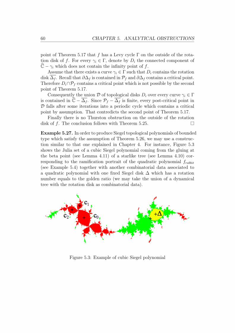
60 CHAPTER 5. ANALYTICAL OBSTRUCTIONS
point of Theorem 5.17 that f has a Levy cycle Γ on the outside of the rota-tion disk of f . For every γi ∈ Γ, denote by Di the connected component ofC− γi which does not contain the infinity point of f .
Assume that there exists a curve γi ∈ Γ such thatDi contains the rotationdisk ∆f . Recall that ∂∆f is contained in Pf and ∂∆f contains a critical point.Therefore Di∩Pf contains a critical point which is not possible by the secondpoint of Theorem 5.17.
Consequently the union D of topological disks Di over every curve γi ∈ Γis contained in C −∆f . Since Pf −∆f is finite, every post-critical point inD falls after some iterations into a periodic cycle which contains a criticalpoint by assumption. That contredicts the second point of Theorem 5.17.
Finally there is no Thurston obstruction on the outside of the rotationdisk of f . The conclusion follows with Theorem 5.25.
Example 5.27. In order to produce Siegel topological polynomials of boundedtype which satisfy the assumption of Theorem 5.26, we may use a construc-tion similar to that one explained in Chapter 4. For instance, Figure 5.3shows the Julia set of a cubic Siegel polynomial coming from the gluing atthe beta point (see Lemma 4.11) of a starlike tree (see Lemma 4.10) cor-responding to the ramification portrait of the quadratic polynomial frabbit(see Example 5.4) together with another combinatorial data associated toa quadratic polynomial with one fixed Siegel disk ∆ which has a rotationnumber equals to the golden ratio (we may take the union of a dynamicaltree with the rotation disk as combinatorial data).
Figure 5.3: Example of cubic Siegel polynomial


Chapter 6
From a tree to a Persian carpet
We have presented different kind of obstructions occuring in realization ofprescribed dynamics by post-critically rational map. In accordance withprevious discussions, we would like now to construct a concrete example ofnon-post-critically rational map whose dynamics is encoded by a sharpeningof a dynamical tree.
6.1 Weighted Hubbard treesWe will push further the discussion began in Section 4.1.
Definition 6.1 (restriction of a planar tree). Let T = (V,E) be a planartree and letW ⊂ V be a subset of vertices. The restriction of T determinedby W is the planar tree T [W ] = (V [W ], E[W ]) where
• V [W ] ⊂ V is the union of vertices in W together with the vertices of Vwhich are in the intersection of at least two Jordan arcs [v, v′]T betweenvertices in W
• E[W ] is the set of Jordan arcs [v, v′]T between vertices in V [W ]
In some sense, the restriction T [W ] is the convex hull of W in T . Recallthat for every dynamical tree T = (T, τ, δ), the dynamical map τ : V → Vcan be extended continuously to T (see Definition 4.3).
Proposition 6.2. Let T = (T, τ, δ) be a dynamical tree. We have:
1. For any Jordan arc [v, v′]T between vertices v, v′ ∈ V containing nocritical point of T except possibly for its endpoints,
τ([v, v′]T ) = [τ(v), τ(v′)]T

CHAPTER 6. FROM A TREE TO A PERSIAN CARPET 63
2. For any subset of vertices W ⊂ V ,
T [τ(W )] ⊂ τ(T [W ]) ⊂ T [τ(W ∪ ΩT )]
Proof of Proposition 6.2. 1. Clearly [τ(v), τ(v′)]T ⊂ τ([v, v′]T ). Now as-sume by contradiction that the previous inclusion is strict. Thereforethere exists an edge outside of [τ(v), τ(v′)]T which belongs to the imagesof at least two edges in [v, v′]T , thus τ|[v,v′]T is not injective. Consider thenonempty set K = (z1, z2) ∈ ([v, v′]T )2 / z1 6= z2 and τ(z1) = τ(z2).Since τ|[v,v′]T is locally injective by assumption (see Definition 4.3), K isa compact set. Take (z1, z2) ∈ K such that |z1− z2| is minimal and letz be a point in the Jordan arc [z1, z2]T distinct from z1 and z2. Noticethat τ(z) is necessarily distinct from τ(z1) = τ(z2) since |z1 − z2| isminimal. Moreover
[τ(z1), τ(z)]T = [τ(z), τ(z2)]T ⊂ τ([z1, z]T ) ∩ τ([z, z2]T )
Hence we can find z′1 ∈ [z1, z]T distinct from z1 and z′2 ∈ [z, z2]T distinctfrom z2 such that τ(z′1) = τ(z′2) contradicting the minimality of |z1−z2|.
2. Since τ is a continuous map, τ(T [W ]) is a convex subset of T containingτ(W ), and so the convex hull T [τ(W )]. Furthermore T [W ] is the unionof Jordan arcs of the form [v, v′]T between endpoints v, v′ ∈ W∪ΩT con-taining no critical point of T except possibly for its endpoints. There-fore the second inclusion follows from the first part.
The proposition above justifies the following definition.
Definition 6.3 (restriction of a dynamical tree). Let T = (T, τ, δ) be adynamical tree and letW ⊂ V such that τ(W )∪ΩT ⊂ W . The restriction ofT determined by W is the dynamical tree T [W ] = (T [W ], τ|T [W ], δ|V [W ])where
• T [W ] = (V [W ], E[W ]) is the restriction of the planar tree T = (V,E)determined by W
• τ|T [W ] : T [W ] → τ(T [W ]) = T [τ(W )] ⊂ T [W ] is the restriction of themap τ on T [W ]
• δ|V [W ] : V [W ]→ N− 0 is the restriction of the map δ on V [W ]

64 CHAPTER 6. FROM A TREE TO A PERSIAN CARPET
Actually the restriction may be seen as the inverse operation of extension(see Definition 4.6) in the sense that T is an extension of T = (T, τ, δ) whereT = (V,E) if and only if T ' T [V ].
Recall that the set of all dynamical trees is partially ordered by (Propo-sition 4.7)
Theorem 6.4. Any dynamical tree has a unique minimal restriction. More-over this dynamical tree is the restriction determined by the union of thecritical and post-critical points.
Proof of Theorem 6.4. Clearly T [ΩT ∪ PT ] is the least element in the set ofall restrictions of T .
Definition 6.5 (abstract Hubbard tree). An abstract Hubbard tree isa minimal restriction H = T [ΩH ∪ PH] of a dynamical tree T of degreedeg(T ) = deg(H) > 2.
Example 6.6. A. Douady and J. H. Hubbard introduced Hubbard tree as-sociated to post-critically finite polynomial in [DH84] as follows. In the filledJulia set K(P ) of a post-critically finite polynomial P , consider Jordan arcssuch that their intersections with any Fatou component (which is necessaryassociated to a super-attracting cycle) consist of the union of finitely manyinternal rays. Then the Hubbard tree associated to P is the smallest closedconnected infinite union of those particular Jordan arcs which contains theunion of critical and post-critical sets of P . A. Douady an J. H. Hubbardproved that this construction is unique and defines a topological tree, calledthe Hubbard tree of P . The action of any post-critically finite polynomialon its associated Hubbard tree provides a family of examples of abstractHubbard trees.
Observe that Hubbard trees of post-critically finite polynomials encodemore informations about dynamical properties than ramification portraits.Actually A. Douady and J. H. Hubbard showed in [DH84] that two non-conformally conjugate post-critically finite polynomials provide two differenttree structures (a Hubbard tree, a dynamics on it coming from the polynomialand a bit of extra information) but they did not give criterion for realization.That was done by A. Poirier in [Poi93] who considered abstract Hubbard treesclose to those of Definition 6.5 but with two more assumptions: one “angled”dynamical property around a certain type of vertices and one expandingcondition. See also [AF00] where the authors study how much of dynamicalinformation about a quadratic Misiurewicz polynomial (whose critical pointis preperiodic) is captured by the Hubbard tree.
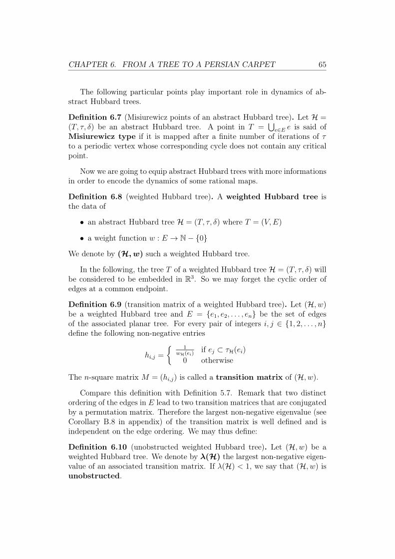
CHAPTER 6. FROM A TREE TO A PERSIAN CARPET 65
The following particular points play important role in dynamics of ab-stract Hubbard trees.
Definition 6.7 (Misiurewicz points of an abstract Hubbard tree). Let H =(T, τ, δ) be an abstract Hubbard tree. A point in T =
⋃e∈E e is said of
Misiurewicz type if it is mapped after a finite number of iterations of τto a periodic vertex whose corresponding cycle does not contain any criticalpoint.
Now we are going to equip abstract Hubbard trees with more informationsin order to encode the dynamics of some rational maps.
Definition 6.8 (weighted Hubbard tree). A weighted Hubbard tree isthe data of
• an abstract Hubbard tree H = (T, τ, δ) where T = (V,E)
• a weight function w : E → N− 0
We denote by (H, w) such a weighted Hubbard tree.
In the following, the tree T of a weighted Hubbard tree H = (T, τ, δ) willbe considered to be embedded in R3. So we may forget the cyclic order ofedges at a common endpoint.
Definition 6.9 (transition matrix of a weighted Hubbard tree). Let (H, w)be a weighted Hubbard tree and E = e1, e2, . . . , en be the set of edgesof the associated planar tree. For every pair of integers i, j ∈ 1, 2, . . . , ndefine the following non-negative entries
hi,j =
1wH(ei)
if ej ⊂ τH(ei)
0 otherwise
The n-square matrix M = (hi,j) is called a transition matrix of (H, w).
Compare this definition with Definition 5.7. Remark that two distinctordering of the edges in E lead to two transition matrices that are conjugatedby a permutation matrix. Therefore the largest non-negative eigenvalue (seeCorollary B.8 in appendix) of the transition matrix is well defined and isindependent on the edge ordering. We may thus define:
Definition 6.10 (unobstructed weighted Hubbard tree). Let (H, w) be aweighted Hubbard tree. We denote by λ(H) the largest non-negative eigen-value of an associated transition matrix. If λ(H) < 1, we say that (H, w) isunobstructed.
66 CHAPTER 6. FROM A TREE TO A PERSIAN CARPET
Example 6.11. Consider the weighted Hubbard tree (H, w) displayed inFigure 6.1. The arrows depict the dynamics of the map τ , and the numbersdepict the weight function w. Hence
τ(eα,c1) = eα,c2τ(eα,c2) = eα,c3τ(eα,c3) = eα,c1
and
w(eα,c1) = 2w(eα,c2) = 2w(eα,c3) = 1
Figure 6.1: Example of unobstructed weighted Hubbard tree
Using the same order of the edges as above, we get the following transitionmatrix of (H, w)
M =
0 12
00 0 1
2
1 0 0
It follows that λ(H) is the largest non-negative root of 4X3 − 1, that is2−2/3 < 1. Therefore (H, w) is unobstructed.
6.2 Weaving by quasiconformal surgery
Consider the weighted Hubbard tree (H, w) displayed in Figure 6.2.The abstract Hubbard tree H = (T, τ, δ) has one fixed branching point
α of Misiurewicz type and one periodic cycle of four vertices c0, c1, c2, c3containing a critical point c0 of local degree δ(c0) = 2. Actually H is theHubbard tree associated to a quadratic polynomial of the form z 7→ z2 + cwhere c ≈ −0.157+1.032i (see Example 6.6). The Julia set of this quadraticpolynomial is drawn in Figure 6.3.
We haveτ(eα,c0) = eα,c1τ(eα,c1) = eα,c2τ(eα,c2) = eα,c0 ∪ ec0,c3τ(ec0,c3) = eα,c1 ∪ eα,c0
and
w(eα,c0) = 1w(eα,c1) = 2w(eα,c2) = 2w(ec0,c3) = 1

CHAPTER 6. FROM A TREE TO A PERSIAN CARPET 67
Figure 6.2: The weighted Hubbard tree (H, w)
Figure 6.3: Hubbard tree of z 7→ z2 − 0.157 + 1.032i
Using the same order for the edges of H as above, we get the followingtransition matrix of (H, w)
M =
0 1 0 00 0 1
20
12
0 0 12
1 1 0 0
An easy computation shows that λ(H) is the largest non-negative root of4X4 − 2X − 1 that is λ(H) ≈ 0.918 < 1. Thus the weighted Hubbard

68 CHAPTER 6. FROM A TREE TO A PERSIAN CARPET
tree (H, w) is unobstructed. We will discuss in Section 6.4 what it happensfor a different choice of weight function w in order that (H, w) is no longerunobstructed.
Now consider the dynamical tree T = (T , τ , δ) deduced from H by re-moving the critical point c0 and by sending c3 to c1 instead of c0, as displayedin Figure 6.4. In some sense, we have deleted the folding point of H.
Figure 6.4: The dynamical tree T deduced from H
We equip T with a weight function w : E → N−0 deduced from w byremoving the weight on ec0,c3 and by keeping that one on eα,c0
w(eα,c3) = 1w(eα,c1) = 2w(eα,c2) = 2
In this way, we get the weighted Hubbard tree of Example 6.11. In particular(H, w) is still unobstructed.
We can easily find a rational map “encoded” by (T , w), that is a rationalmal which realizes the ramification portrait R below where the degrees comefrom the weight function w on the corresponding edges.
c12 // c2
2 // c3
1
gg
Indeed choosing c1 = 1, c2 = ∞ and c3 = 0, this ramification portrait isrealized by the map z 7→ z2 precomposed with a Möbius transformation

CHAPTER 6. FROM A TREE TO A PERSIAN CARPET 69
which acts as a circular permutation on 0, 1,∞:
f =(z 7→ z2
)(z 7→ 1
1− z
)=
(z 7→ 1
(1− z)2
)The Julia set of f is drawn in Figure 6.5. This Julia set plays an importantrole in the Hubbard’s twisted rabbit problem disccussed in Example 5.4.
Figure 6.5: The Julia set of f
Now we are going to explain more precisely how f is “encoded” by (T , w).To do so, for any point c in the attracting cycle 0, 1,∞ of f , consider B(c)the connected component containing c of the immediate attracting bassin(i.e. the set of points whose forward orbits accumulate the super-attractingcycle containing c). A classical result in holomorphic dynamical systemsclaims that f 3|B(c) : B(c) → B(c) is conjugated to (z 7→ z4) : D → D by abiholomorphic map φc, called the Böttcher coordinates (the φc are unique upto multiplication by a third root of unity), with φc(c) = 0. Furthermore theφc together for c ∈ 0, 1,∞ make the following diagram commutative:
B(0)φ0 //
f
D
z 7→ z
B(1)φ1 //
f
D
z 7→ z2
B(∞)
φ∞ //
f
D
z 7→ z2
B(0)
φ0 // D

70 CHAPTER 6. FROM A TREE TO A PERSIAN CARPET
Then define a map π : C→ T = eα,c3 ∪ eα,c1 ∪ eα,c2 ⊂ C as follows
π : z 7→
|φ0(z)|α + (1− |φ0(z)|)c3 ∈ eα,c3 if z ∈ B(0)|φ1(z)|α + (1− |φ1(z)|)c1 ∈ eα,c1 if z ∈ B(1)|φ∞(z)|α + (1− |φ∞(z)|)c2 ∈ eα,c2 if z ∈ B(∞)
α otherwise
In this way, π is a continuous and surjective map such that the preimageof each point of T − α is an equipotential (i.e. a preimage of a circlecentered at the origin by the Böttcher coordinates). Moreover we may finda suitable continuous extension of τ : V → V to T in Definition 4.3 in orderto make the following diagram commutative (see Figure 6.6)⋃
B(c) π //
f
T
τ⋃
B(c)π
// T
Figure 6.6: f is encoded by (T , w)
Actually define τ as follows
τ : x 7→
µα + (1− µ)c1 ∈ eα,c1 if x = µα + (1− µ)c3 ∈ eα,c3µ2α + (1− µ2)c2 ∈ eα,c2 if x = µα + (1− µ)c1 ∈ eα,c1µ2α + (1− µ2)c3 ∈ eα,c3 if x = µα + (1− µ)c2 ∈ eα,c2
α otherwise

CHAPTER 6. FROM A TREE TO A PERSIAN CARPET 71
Heuristically speaking, we may think of the action of f on⋃B(c) as that
one of τ on the boundary of a small “thickening” of the tree T embedded inR3 as it is suggested in Figure 6.6.
Now we would like to construct a rational map f whose dynamics is en-coded by the weighted Hubbard tree (H, w). To do so, we start with therational map f and we create a kind of “folding” point c0 inside B(0) (whichcorresponds to the edge eα,c3) by a surgery process. More precisely, we aregoing to divide the Riemann sphere C into several pieces whose boundariesare equipotentials, and then we will define a continuous and sufficiently reg-ular map F : C→ C which is encoded by (H, w) as a piecewise map. Finallythe quasiconformal surgery principle (see Theorem C.13 in appendix) willprovide us a rational map f as required.
Step 1 - Cutting off For every c ∈ 0, 1,∞, denote by αc the boundaryof B(c) (recall that B(c) is a topological disk since it is biholomorphicallymapped onto the unit disk D).
We follow the notations of Definition C.4 in appendix: for any pair ofdisjoint continua γ and γ′, we denote by A(γ, γ′) the unique doubly connectedcomponent of C− (γ ∪ γ′) and by mod(γ, γ′) > 0 its modulus. In particularif γ and γ′ are two equipotentials of levels |φc(γ′)| < |φc(γ)| in B(c) for anyc ∈ 0, 1,∞, then
mod(γ, γ′) =1
2πlog
(|φc(γ)||φc(γ′)|
)Lemma 6.12. Given any positive constant C > 0, there exist five equipoten-tials β0, β1, β2, γ−3 and γ+3 such that
(i) β0 ⊂ B(0), β1 ⊂ B(1) and β2 ⊂ B(2)
(ii) γ−3, γ+3 ⊂ B(0) and |φ0(β0)| > |φ0(γ−3)| > |φ0(γ+3)|
(iii) the following inequalities holdmod(α1, β1) < mod(α0, β0)
12
mod(α2, β2) < mod(α1, β1)12
mod(α0, β0) + 12
mod(γ−3, γ+3) < mod(α2, β2)mod(α0, β0) + mod(α1, β1) + C < mod(γ−3, γ+3)
(6.1)
12
mod(α0, γ+3) < mod(α2, β2) (6.2)

72 CHAPTER 6. FROM A TREE TO A PERSIAN CARPET
If β′2,0, β′0,1, β′1,2, γ′2,−3 and γ′2,+3 denote the equipotentials which are therespective preimages by g of β0, β1, β2, γ−3 and γ+3 then the previous in-equalities implies (see Proposition C.5 in appendix)
|φ0(β′0,1)| > |φ0(β0)| > |φ0(γ−3)| > |φ0(γ+3)||φ1(β′1,2)| > |φ1(β1)||φ∞(β′2,0)| > |φ∞(γ′2,−3)| > |φ∞(γ′2,+3)| > |φ∞(β2)|
The pattern of those equipotentials on C are displayed in Figure 6.7.
Figure 6.7: Equipotentials in Lemma 6.12
Proof of Lemma 6.12. Compare the inequalities (6.1) with the transition ma-trix of the weighted Hubbard tree (H, w):
M =
0 1 0 00 0 1
20
12
0 0 12
1 1 0 0
By Corollary B.8 in appendix and since λ(H) < 1, there exists a vectorx ∈ R4 with positive entries such that Mx < x. Let µ > 0 be large enoughsuch that
Mµx+
000C
< µx (6.3)
Let β0 ⊂ B(0), β1 ⊂ B(1) and β2 ⊂ B(2) be three equipotentials such that
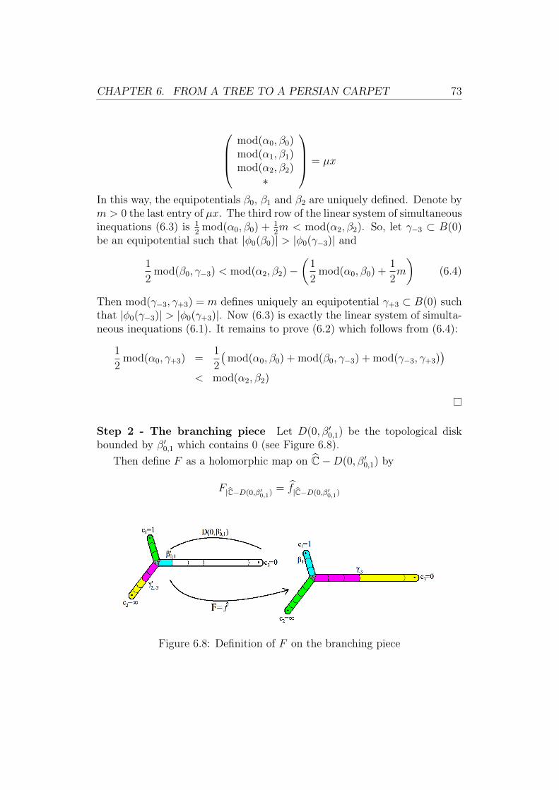
CHAPTER 6. FROM A TREE TO A PERSIAN CARPET 73
mod(α0, β0)mod(α1, β1)mod(α2, β2)
∗
= µx
In this way, the equipotentials β0, β1 and β2 are uniquely defined. Denote bym > 0 the last entry of µx. The third row of the linear system of simultaneousinequations (6.3) is 1
2mod(α0, β0) + 1
2m < mod(α2, β2). So, let γ−3 ⊂ B(0)
be an equipotential such that |φ0(β0)| > |φ0(γ−3)| and
1
2mod(β0, γ−3) < mod(α2, β2)−
(1
2mod(α0, β0) +
1
2m
)(6.4)
Then mod(γ−3, γ+3) = m defines uniquely an equipotential γ+3 ⊂ B(0) suchthat |φ0(γ−3)| > |φ0(γ+3)|. Now (6.3) is exactly the linear system of simulta-neous inequations (6.1). It remains to prove (6.2) which follows from (6.4):
1
2mod(α0, γ+3) =
1
2
(mod(α0, β0) + mod(β0, γ−3) + mod(γ−3, γ+3)
)< mod(α2, β2)
Step 2 - The branching piece Let D(0, β′0,1) be the topological diskbounded by β′0,1 which contains 0 (see Figure 6.8).
Then define F as a holomorphic map on C−D(0, β′0,1) by
F|C−D(0,β′0,1) = f|C−D(0,β′0,1)
Figure 6.8: Definition of F on the branching piece

74 CHAPTER 6. FROM A TREE TO A PERSIAN CARPET
Step 3 - Preimage of the branching piece Recall the last inequality ofthe system of simultaneous inequations (6.1)
mod(α0, β0) + mod(α1, β1) + C < mod(γ−3, γ+3)
We have not fixed the value of the positive constant C yet. By a result of CuiGuizhen and Tan Lei in [CT07] (see Lemma C.7 in appendix) there existsC > 0 such that for every pair of equipotentials β0 ⊂ B(0) and β1 ⊂ B(1),
mod(β1, β0) < mod(α0, β0) + mod(α1, β1) + C
For this C, apply the Lemma 6.12. We get as a consequence
mod(β1, β0) < mod(γ−3, γ+3)
Therefore we can find two equipotentials β′−3,1 and β′+3,0 in B(0) suchthat
|φ0(γ−3)| > |φ0(β′−3,1)| > |φ0(β′+3,0)| > |φ0(γ+3)|
mod(β′−3,1, β′+3,0) = mod(β1, β0)
These two equipotentials are displayed in Figure 6.9.
Figure 6.9: Realization of a preimage of the branching piece
Now define F on A(β′−3,1, β′+3,0) to be any biholomorphic map such that
• F maps A(β′−3,1, β′+3,0) onto A(β1, β0)
• F extends diffeomorphically to A(β′−3,1, β′+3,0) mapping β′−3,1 onto β1
and β′+3,0 onto β0

CHAPTER 6. FROM A TREE TO A PERSIAN CARPET 75
Step 4 - Folding We are going to realize the folding point c0 of H bycreating some critical points of F in A(β′0,1, β
′−3,1).
Lemma 6.13. There exists a biholomorphic map ϕ mapping A(β0, γ−3) ontoan annulus of the form Ar = z ∈ C / r < |z| < 1
r where r ∈]0, 1[ and having
a diffeomorphical extension to A(β0, γ−3).
Proof of Lemma 6.13. Consider the composition map below
ϕ = (z 7→ µz)φ0 : A(β′0,1, β′−3,1)→ z ∈ D / µ|φ0(β′−3,1)| < |z| < µ|φ0(β′0,1)|
with µ = 1/√|φ0(β0)||φ0(γ−3)| and take ϕ = ϕ|A(β0,γ−3).
The aim is now to map the annulus Ar onto a topological disk.
Figure 6.10: Creation of some critical points
Consider the rational map (z 7→ z + 1z) on Ar. It has two simply critical
points 1 and -1 and it maps Ar onto an ellipse denoted by εr. Denote by p(respectively p′) the unique preimage of the critical point 1 (respectively -1)by ϕ.
Now let ξ be an equipotential in B(1) such that |φ1(β1)| > |φ1(ξ)| anddenote D(1, ξ) the topological disk bounded by ξ which contains 1. Let ψ beany biholomorphic map such that ψ(εr) = D(1, ξ), ψ(2) = 1 and ψ extendsdiffeomorphically to εr. All the process is resumed in Figure 6.10.
Finally define F as a holomorphic map on A(β0, γ−3) by
F|A(β0,γ−3) = ψ (z 7→ z +1
z) ϕ
Notice that F extends diffeomorphically to the boundary ∂A(β0, γ−3). More-over F has now two new critical points p and p′. The first one c0 = p is sentexactly to c1 = 1 (in the future super-attracting cycle) and the second onep′ is sent near 1 (more precisely in D(1, ξ) ⊂ B(1)).

76 CHAPTER 6. FROM A TREE TO A PERSIAN CARPET
Figure 6.11: Realization of the folding
On the remaining annuliA(β′0,1, β0) andA(γ−3, β′−3,1), just extend quasireg-ularly F mapping A(β′0,1, β0) and A(γ−3, β′−3,1) onto A(β1, ξ) (see PropositionC.12 in appendix). Figure 6.11 illustrates how F realizes a folding point atthe new critical point c0 = p.
Step 5 - End with an end It remains to define F on the topologicaldisk D(0, β′+3,0) (see Figure 6.12). The main difficulty is that this domainmust contain a preimage of itself in order for F to be encoded by (H, w) asrequired.
Figure 6.12: Realization of a preimage of an end
Let δ′+3,−3 be a smooth curve (i.e. the image of the unit circle S1 by adiffeomorphism) in A(β′+3,0, γ+3) which does not separate β′+3,0 and γ+3 (i.e.they are both in the same connected component of C − δ′+3,−3). Denote byD(δ′+3,−3) the connected component of C− δ′+3,−3 disjoint with β′+3,0 ∪ γ+3.

CHAPTER 6. FROM A TREE TO A PERSIAN CARPET 77
Define F on D(δ′+3,−3) to be any biholomorphic map such that
• F maps D(δ′+3,−3) onto D(0, γ−3)
• F extends diffeomorphically to D(δ′+3,−3) mapping δ′+3,−3 onto γ−3
In this way, we have realized a preimage of D(0, γ−3) (see Figure 6.12). Nowwe are going to realize the mapping of the end c3 = 0 to the folding pointc0 = p.
Figure 6.13: The map F on the whole Riemann sphere
Let ζ be a smooth curve in A(β0, γ−3) which does not separate β0 and γ−3
such that the connected component of C− ζ disjoint with β0 ∪ γ−3, denotedby D(p, ζ), contain the critical point p but not the critical point p′ (see Figure6.13).
Define F on D(0, γ+3) to be any biholomorphic map such that
• F maps D(0, γ+3) onto D(p, ζ)
• F (0) = p
• F extends diffeomorphically to D(0, γ+3) mapping γ+3 onto ζ
Finally let P (β′+3,0, δ′+3,−3, γ+3) be the remaining pair of pants bounded by
β′+3,0, δ′+3,−3 and γ+3 and let P (β0, γ−3, ζ) be as well. Extend quasiregularly Fto P (β′+3,0, δ
′+3,−3, γ+3) mapping P (β′+3,0, δ
′+3,−3, γ+3) onto P (β0, γ−3, ζ) (see
Proposition C.12).Figure 6.13 shows the entire piecewise definition of F on C.
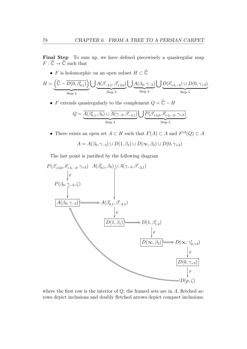
78 CHAPTER 6. FROM A TREE TO A PERSIAN CARPET
Final Step To sum up, we have defined piecewisely a quasiregular mapF : C→ C such that
• F is holomorphic on an open subset H ⊂ C
H =(C−D(0, β′0,1)
)︸ ︷︷ ︸
Step 2
⋃A(β′−3,1, β
′+3,0)︸ ︷︷ ︸
Step 3
⋃A(β0, γ−3)︸ ︷︷ ︸
Step 4
⋃D(δ′+3,−3) ∪D(0, γ+3)︸ ︷︷ ︸
Step 5
• F extends quasiregularly to the complement Q = C−H
Q = A(β′0,1, β0) ∪ A(γ−3, β′−3,1)︸ ︷︷ ︸Step 4
⋃P (β′+3,0, δ
′+3,−3, γ+3)︸ ︷︷ ︸
Step 5
• There exists an open set A ⊂ H such that F (A) ⊂ A and F 2(Q) ⊂ A
A = A(β0, γ−3) ∪D(1, β1) ∪D(∞, β2) ∪D(0, γ+3)
The last point is justified by the following diagram
P (β′+3,0, δ′+3,−3, γ+3)
F
A(β′0,1, β0) ∪ A(γ−3, β′−3,1) _
P (β0, γ−3, ζ) _
A(β0, γ−3) +3 A(β′0,1, β
′−3,1)
F
D(1, β1) +3 D(1, β′1,2)
F
D(∞, β2) +3 D(∞, γ′2,+3)
F
D(0, γ+3)
F
D(p, ζ)> ^
RZ
where the first row is the interior of Q, the framed sets are in A, fletched ar-rows depict inclusions and doubly fletched arrows depict compact inclusions.

CHAPTER 6. FROM A TREE TO A PERSIAN CARPET 79
We may thus apply the Shishikura’s principle on quasiconformal surgery(see Theorem C.13 in appendix) to get a F -invariant almost complex struc-ture. Therefore F is conjugated by a quasiconformal map (coming from themeasurable Riemann’s mapping theorem C.10) to a rational map f on C.In particular f is still “encoded” by the weighted Hubbard tree (H, w) asrequired. Notice that f is non-post-critically finite since the forward orbit ofthe new critical point p′ is infinite.
6.3 Pictures
In general such a construction does not provide an algebraic formula forthe rational map we obtain. Since we add critical points by quasiconformalsurgery to some rational map, the degree increases quickly as soon as werequire a sufficiently interesting tree structure. So the algebraic relationsbehind such examples are complicated to study. However the particularweighted Hubbard tree (H, w) of the previous section is simple enough toprovide an algebraic formula for such a rational map fp depending on thecritical point p ∈ C.
Recall at first that fp realizes asymptotically (see Definition 3.12) theramification portrait below.
p2 // 1 2 //∞ 2 // 0
1
ii p′2 // 1
The last arrow means that the critical point p′ is mapped in the connectedcomponent containing 1 of the immediate attracting bassin of fp. Remarkthat fp has four critical points of multiplicity one and then deg(fp) = 3 (byRiemann-Hurwitz formula). In particular fp is of the form
fp : z 7→ az3 + bz2 + cz + d
Az3 +Bz2 + Cz +D
Since 1 is mapped to∞ with a local degree two, the denominator may factoras
fp : z 7→ az3 + bz2 + cz + d
(z − 1)2(C ′z +D′)
We do likewise for ∞ which is mapped to 0 with a local degree two
fp : z 7→ cz + d
(z − 1)2(C ′z +D′)

80 CHAPTER 6. FROM A TREE TO A PERSIAN CARPET
Now use the fact that fp(0) = p to get
fp : z 7→ cz + p
(z − 1)2(C ′z + 1)
It remains two informations fp(p) = 1 and f ′p(p) = 0 which lead to twoequations satisfied by c and C ′
(1− p)2(pC ′ + 1) = p(c+ 1)
c(1− p)2(pC ′ + 1) = p(c+ 1)((1− 4p+ 3p2)C ′ − 2 + 2p)
Remark that we may easily simplify the second equation by using the firstone (luckily). Then we get the following linear system of two equations
pc− p(1− p)2C ′ = 1− 3p+ p2
c− (1− p)(1− 3p)C ′ = −2 + 2p
Finally we obtain c =−1 + 4p− 6p2 + p3
2p2
C ′ =−1 + p+ p2
2p2(1− p)and
fp : z 7→(1− p)
[(−1 + 4p− 6p2 + p3)z + 2p3
](z − 1)2
[(−1 + p+ p2)z + 2p2(1− p)
]Some more computations provide an algebraic formula for the last critical
point depending on the position of the first one
p′ =−p(5p4 − 10p3 + 11p2 − 6p+ 1
)(p2 + p− 1
)(p3 − 6p2 + 4p− 1
)We have proved in the previous section that there exist some choices of p
(in order to make fp(p′) close to 1) such that fp is “encoded” by the weightedHubbard tree (H, w). Indeed for p ≈ −0.0005 we get the bifurcation locusin Figure 6.14.

CHAPTER 6. FROM A TREE TO A PERSIAN CARPET 81
Figure 6.14: The hyperbolic component of the family (fp)p∈Cinside a disk of center −0.0005 and radius 0.005
Picking a parameter p inside the big hyperbolic component, we obtainthe Julia set J (fp) in Figure 6.16 called a Persian carpet.
Observe that the Julia set of f is displayed as a “watermark” or moreprecisely as a buried Julia component inside J (fp) (compare with Figure6.5). Actually this Julia component is fixed, and it’s the only one periodicJulia component with a complicated topology. More precisely Tan Lei andK. Pilgrim proved in [PT00] that except for this fixed Julia component andits countable collection of preimages, every Julia component of J (fp) is apoint or a Jordan curve (see Theorem 6.14).

82 CHAPTER 6. FROM A TREE TO A PERSIAN CARPET
Figure 6.15: The weighted Hubbard tree (H, w) which encodes fp
Figure 6.16: The Julia set of f−0.0005 which is encoded by (H, w)

CHAPTER 6. FROM A TREE TO A PERSIAN CARPET 83
Theorem 6.14 (Tan Lei-Pilgrim). Let f : C → C be a rational map withdisconnected Julia set J (f). Denote by P ′f the accumulation set of its post-critical set. The following holds.
1. If P ′f ∩J (f) is finite then every wandering Julia component is a pointor a Jordan curve.
2. If P ′f ∩J (f) is contained in finitely many Julia components then everywandering Julia component is either simply or doubly connected.
See also [CPT09] for a sharpening of this result.With regards to the Fatou components, they are preimages of the imme-
diate attracting bassin of fp shown in Figure 6.17.
Figure 6.17: Some details of a Persian carpet

84 CHAPTER 6. FROM A TREE TO A PERSIAN CARPET
6.4 CounterexampleLet us come back to the beginning of the construction in Section 6.2. Nowequip the abstract Hubbard tree H with the following weight function:
w′(eα,c0) = 1w′(eα,c1) = 1w′(eα,c2) = 2w′(ec0,c3) = 1
We deduce the following transition matrix of (H, w′)
M ′ =
0 1 0 00 0 1 012
0 0 12
1 1 0 0
λ′(H) is the largest non-negative root of 2X4−2X−1 that is λ′(H) ≈ 1.130.Thus the new weighted Hubbard tree (H, w′) is no longer unobstructed.
However we may try to carry out the same construction. The first diffi-culty comes from Lemma 6.12 but we may overcome it. For instance, definefive equipotentials which satisfy the conditions (i), (ii) together with thelinear system of simultaneous inequations (6.1) but not the inequation (6.2)(see Proof of Lemma 6.12).
After that all is right until the final step. There the big diagram is nolonger true. Indeed the compact inclusion D(∞, ζ2) ⊂ D(∞, δ2) which camefrom the inequation (6.2) does not hold any more. So we cannot applythe Shishikura’s principle on quasiconformal surgery and the constructionprovides only a quasiregular map which is not necessarily quasiconformallyconjugated to a rational map.
Actually a result of C. T. McMullen from [McM94] implies that such arational map does not exist.
Theorem 6.15 (McMullen). Let f be a rational map which is not a Lattèsexample (i.e. whose Fatou set F(f) is nonempty). Assume that there existsa Thurston obstruction Γ. Then λ(fΓ) = 1 and at least one curve in themulti-curve Γ is contained in the union of Fatou components where f isbiholomorphically conjugated to a rotation.
In our case, every critical points accumulate a super-attracting cycle andconsequently every Fatou component is a preimage of a connected componentof the immediate attracting bassin. In particular there is no rotation domainin the Fatou set.

CHAPTER 6. FROM A TREE TO A PERSIAN CARPET 85
Therefore the assumption of unobstructed weighted Hubbard tree is re-quired in order to complete the construction of Section 6.2 successfully.
In particular, remark that the choice of weight function w in Section 6.2is the simplest possible to make the abstract Hubbard tree H unobstructed.
6.5 EncodingWe conclude this section by showing how the exchanging dynamics of Juliacomponents induced by the rational map f constructed in Section 6.2 is“encoded” by the weighted Hubbard tree (H, w).
Figure 6.18: Some annuli
We follow the notations from Section 6.2. We consider the followingannuli (see Figure 6.18):
• For every k ∈ 0, 1, 2, A′k = A(αk, β′k,k+1) (with the notation β′2,3 =
β′2,0) and Ak = A(αk, βk)
• A′3 = A(β′−3,1, β′+3,0) and A3 = A(γ−3, γ+3)
• A′γ = A(γ′2,−3, γ′2,+3)
We have:
1. (topology) For every k ∈ 0, 1, 2, 3, A′k ⊂ Ak and A′γ ⊂ A2.
2. (dynamics) The following restrictions are unbranched coverings:
F|A′0 : A′0 → A1 , F|A′1 : A′1 → A2 , F|A′2 : A′2 → A0
F|A′γ : A′γ → A3 , F|A′3 : A′3 → A(β1, β0) ⊃ A1 ∪ A0

86 CHAPTER 6. FROM A TREE TO A PERSIAN CARPET
Now we consider as well open sets on the associated Hubbard tree H =(T, τ, δ). Recall that T is the union of four edges which are isometric tofour segments denoted by eα,c0 = [α, c0], eα,c1 = [α, c1], eα,c2 = [α, c2] andec0,c3 = [c0, c3] (see Figure 6.3).
Lemma 6.16. There exist open segments in T of the form
• For every k ∈ 0, 1, 2, I ′k =]α, b′k,k+1[⊂ eα,ck (with the notation b′2,3 =b′2,0) and Ik =]α, bk[⊂ eα,ck
• I ′3 =]b′−3,1, c0] ∪ [c0, b′+3,0[⊂ eα,c0 ∪ ec0,c3 and I3 =]g−3, c0] ∪ [c0, g+3[⊂
eα,c0 ∪ ec0,c3
• I ′γ =]g2,−3, g2,+3[⊂]b′2,0, c2[⊂ eα,c2 − I ′2and a suitable continuous extension of τ : V → V to T in Definition 4.3 suchthat
1. (topology) For every k ∈ 0, 1, 2, 3, I ′k ⊂ Ik and I ′γ ⊂ I2.
2. (dynamics) The following restrictions are surjective affine maps:
τ|I′0 : I ′0 → I1 , τ|I′1 : I ′1 → I2 , τ|I′2 : I ′2 → I0
τ|I′γ : I ′γ → I3 , τ|I′3 : I ′3 → I1 ∪ α ∪ I0
3. (expansion) the set
JH = x ∈ T / (τ n(x))n>1 does not accumulate c0, c1, c2, c3
is a Cantor set which is equal to
JH = x ∈ T /∀n > 1, τ n(x) ∈ α ∪ I ′0 ∪ I ′1 ∪ I ′2 ∪ I ′γ ∪ I ′3
Remark that the intersection between the Hubbard tree and the Julia setof the quadratic polynomial in Figure 6.3 is well a Cantor set. Actually thisintersection is homeomorphic to JH and the dynamics is conjugated to τ .
Proof of Lemma 6.16. At first, we may easily consider open segments satis-fying the assumptions together with the first condition (topology). Moreoverwe may require that every new picked points on boundaries of the segmentsare not in V = α, c0, c1, c2, c3 and every inclusions in the first condition arecompact. Define τ on the new picked points by
τ(b′0,1) = b1, τ(b′1,2) = b2, τ(b′2,0) = b0
τ(b′−3,1) = b1, τ(b′+3,0) = b0
τ(g2,−3) = g−3, τ(g2,+3) = g+3

CHAPTER 6. FROM A TREE TO A PERSIAN CARPET 87
Recall the definition of τ on V
τ(c0) = c1, τ(c1) = c2, τ(c2) = c3, τ(c3) = c0 and τ(α) = α
Now extend continuously τ on T by linear interpolation. We get easily thesecond condition (dynamics) and we may classically check the third one (ex-pansion) (see for instance [Bea91] or [Mil06]).
Given a point x ∈ JH, we may look at its itinerary that is the iterativeaddress relative to the set of intervals I ′0, I ′1, I ′2, I ′γ, I ′3. This motivates theassociation of the following symbolic dynamical system (Σ, σ):
• Σ = ε ∈ 0, 1, 2, γ, 3N /∀i ∈ N, εiεi+1 ∈ 01, 12, 20, γ3, 30, 31
• σ : Σ→ Σ is the shift map that is ∀ε ∈ Σ, σ(ε0ε1ε2 . . . ) = ε1ε2ε3 . . .
More precisely (Σ, σ) is a subshift of finite type. Classically we may equip Σwith a metric dΣ so that Σ is a Cantor set and σ is continuous (see [Bea91]or Chapter 2).
Lemma 6.17. There is a continuous semi-conjugacy ψ : (Σ, σ) → (JH, τ)that is a continuous and surjective map making the following diagram com-mutative
Σ σ //
ψ
Σ
ψ
JH τ// JH
such that
(i) for every ε = ε0ε1ε2 · · · ∈ Σ we haveψ(ε) ∈ I ′ε0 ∪ α if ε0 ∈ 0, 1, 2ψ(ε) ∈ I ′γ if ε0 = γψ(ε) ∈ I ′3 if ε0 = 3
(ii) ψ−1(α) = 012, 120, 201
(iii) for any inverse image x ∈⋃n>1 τ
−n(α),
ψ−1(x) = µ3012, µ3120, µ3201
where µ ∈ 0, 1, 2, γ, 3N is a finite word of length N > 0
(iv) for any other x ∈ JH −⋃n>0 τ
−n(α), ψ−1(x) is a unique point in Σ

88 CHAPTER 6. FROM A TREE TO A PERSIAN CARPET
Proof of Lemma 6.17. We give only the main ideas of the proof. Considerthe following inverse branches (by Lemma 6.16):
(τ|I′0)−1 : I1 → I ′0 , (τ|I′1
)−1 : I2 → I ′1 , (τ|I′2)−1 : I0 → I ′2
(τ|I′γ )−1 : I3 → I ′γ , (τ|I′3
)−1 : I1 ∪ I0 → I ′3
Then given any ε ∈ Σ the following intersection
+∞⋂i=0
[(τ|I′ε0
)−1 (τ|I′ε1)−1 · · · (τ|I′εi−1
)−1]
(I ′εi)
is reduced to exactly one point x in JH as decreasing sequence of nonemptycompact subsets with diameters tending to zero. Now define ψ(ε) = x andthe remaining follows.
Similarly define JH(F ) to be the set of connected components of thefollowing non-escaping set
z ∈ C / ∀n > 0, F n(x) ∈ Jα ∪ A′0 ∪ A′1 ∪ A′2 ∪ A′γ ∪ A′3 −D′3,2
where Jα is the Julia set of f (see Figure 6.5) and D′3,2 is the unique topo-logical disk which is mapped by F onto the connected component of thecomplement of Jα containing c2 =∞ (denoted by D(∞, α2) according to ournotations). D′3,2 is shown in Figure 6.18.
We equip JH(F ) −⋃n>0 F
−n(Jα) with the Hausdorff topology comingfrom the following Hausdorff metric:
∀J, J ′ ∈ JH(F )−⋃n>0
F−n(Jα),
dH(J, J ′) = max
supz∈J
infz′∈J ′|z − z′|, sup
z′∈J ′infz∈J|z − z′|
We add to this topology some neighbourhoods of each component J ∈ JH(F )mapped onto Jα after some iterations of F defined as follows
∀k > 1, V1/k(J) =
J ′ ∈ JH(F ) , inf
z∈J,z′∈J ′|z − z′| < 1
k
In this way, JH(F ) is a topological space on where F induces a continuousdynamical system denoted also by F : JH(F )→ JH(F ).

CHAPTER 6. FROM A TREE TO A PERSIAN CARPET 89
Remark that the forward orbit of every component J ∈ JH(F ) does notaccumulate the attracting cycle c0 = p, c1 = 1, c2 = ∞, c3 = 0. Butthere exist some more points in C with this property. For instance, somecomponents in JH(F ) have preimages by F in the forgotten topological diskD′3,2 or in the topological disk D(δ′+3,−3) (see Step 5 in Section 6.2). We willnot discuss the dynamics of such points in D′3,2 ∪D(δ′+3,−3) and all of theirpreimages.
Nevertheless we have the following result whose proof is similar to thatone of Lemma 6.17.
Lemma 6.18. There is a continuous semi-conjugacy φ : (Σ, σ)→ (JH(F ), F )such that
(i) for every ε = ε0ε1ε2 · · · ∈ Σ we haveφ(ε) ⊂ A′ε0 ∪ Jα if ε0 ∈ 0, 1, 2φ(ε) ⊂ A′γ if ε0 = γφ(ε) ⊂ A′3 if ε0 = 3
(ii) φ−1(Jα) = 012, 120, 201
(iii) for any component J ∈ JH(F ) mapped onto Jα after some iterationsof F ,
φ−1(J) = µ3012, µ3120, µ3201
where µ ∈ 0, 1, 2, γ, 3N is a finite word of length N > 0
(iv) for any other component J ∈ JH(F ), φ−1(J) is a unique point in Σ
Recall that F is conjugated by a quasiconformal map to the rationalmap f on C. Therefore the same result holds for the subset JH(f) of Juliacomponents of f which correspond quasiconformally to the components inJH(F ). JH(f) is equipped with a topology induced from that one of JH(F ).Hence we get a semi-conjugacy ϕ : Σ → JH(f) which is quasiconformallyconjugated to φ. That allows to encode every Julia components in JH(f) asin Lemma 6.18.

90 CHAPTER 6. FROM A TREE TO A PERSIAN CARPET
Finally the following result about the encoding of a subset of Julia com-ponents of f folllows easily from Lemma 6.17 and Lemma 6.18 together withTheorem 6.14.
Theorem 6.19. There is a continuous semi-conjugacy ϕ : (Σ, σ)→ (JH(f), f)such that
(i) ψ ϕ−1 : (JH(f), f)→ (JH, τ) is a conjugacy that is a continuous andbijective map making the following diagram commutative
JH(f)f //
ψ ϕ−1
JH(f)
ψ ϕ−1
JH τ
// JH
(ii) for any Julia component J ∈ JH(f), it is a Jordan curve if and onlyif ϕ−1(J) is a unique point in Σ, in other words if and only if it is notmapped after some iterations of f onto the fixed Julia component whichcorresponds quasiconformally to Jα


Chapter 7
A collection of Persian carpets
Now we would like to generalize the construction of the previous chapterin order to get a large family of non-post-critically rational maps encodedby weighted Hubbard trees. As a consequence, we obtain a result aboutrealization of some particular infinite ramification portraits. We will concludeby some computable examples.
7.1 General construction
As the particular construction in Section 6.2, we would like to constructpiecewisely a map F . But we will use a result of Cui Guizhen and Tan Leiinstead of a quasiconformal surgery method to conclude. That allows us toconstruct a map F which is required to be less regular than a quasiregularmap. Nevertheless we keep in head that the aim (the final rational map f)is similar to that one in Section 6.2.
Step 0 - The starting data At first we need a post-critically map f“encoded” by a particular weighted Hubbard tree (T , w) deduced from aweighted Hubbard tree (H, w) by removing some critical points as in thebeginning of the construction in Section 6.2. In other words, we would liketo start the construction by a rational map f which realizes a given finiteramification portrait R. But it is not a so easy task. Actually we havealready discussed in Chapter 4 and Chapter 5 the obstructions that couldarise. In particular Corollary 5.21 ensures that we may find such a post-critically rational map f if the ramification portrait R is N -cyclic where Nis a positive integer.
This assumption is not necessary. Although we have seen in Section 4.3that we may find another sufficient condition for a larger class of ramification

94 CHAPTER 7. A COLLECTION OF PERSIAN CARPETS
portraits which are realized by ramified coverings, the discussions in Chapter5 showed that the analytical part of the problem does not provide an easyto check criterion in general. Therefore we restrict here the issue to N -cyclicramification portraits. That will lead to a large enough family of rationalmaps.
Let N be a positive integer and let R be a N -cyclic ramification portraitdenoted by
c11
ν(c11)// c1
2
ν(c12)// . . .
ν(c1n1−1)// c1n1
ν(c1n1 )
ll
c21
ν(c21)// c2
2
ν(c22)// . . .
ν(c2n2−1)// c2n2
ν(c2n2 )
ll
......
cN1ν(cN1 )
// cN2ν(cN2 )
// . . .ν(cNnN−1)
// cNnNν(cNnN
)
ll
c∞ deg(R)jj
Without loss of generality, we may write the last cycle like the previous oneswith notations nN+1 = 1, cN+1
1 = c∞ and ν(cN+11 ) = deg(R). Notice that
(1) ∀i ∈ 1, 2, . . . , N, ∃k ∈ 1, 2, . . . , ni / ν(cik) > 2
(2) ν(cN+11 ) = 1 +
∑i∈1,2,...,N
(∑k∈1,2,...,ni(ν(cik)− 1)
)Let f be a rational map realizing the ramification portrait R. We follow
notations from Section 6.2: for every integers i ∈ 1, 2, . . . , N + 1 andk ∈ 1, 2, . . . , ni denote by B(cik) the connected component containing cikof the immediate attracting bassin of the ith cycle and by φcik the associatedBöttcher coordinates. We may show as in Section 6.2 that the action of f isencoded by a weighted Hubbard tree (T , w), that is there exist a continuousand surjective map π : C → T and a suitable continuous extension of τ :V → V to T in Definition 4.3 such that the following diagram is commutative⋃
B(cik)π //
f
T
τ⋃
B(cik) π// T

CHAPTER 7. A COLLECTION OF PERSIAN CARPETS 95
Indeed the weighted Hubbard tree (T , w) is a starlike tree, that is a treeformed by the set of vertices V = α ∪ (
⋃cik) where α is the unique
branching point and by the set of edges E = Eα =⋃eα,cik (recall that a
weighted Hubbard tree is considered to be embedded in R3 and thus withoutcyclic order of edges at a common endpoint), whose dynamics τ fixes thebranching point α and acts as the dynamics σ of R on the ends cik andwhose weight function w is deduced from the local degrees function ν of R:
∀i ∈ 1, 2, . . . , N + 1,∀k ∈ 1, 2, . . . , ni, w(eα,cik) = ν(cik)
Recall that we would like to construct a rational map f from f which hastwo new critical points inside some B(cini), say pi and p
′i. In other words, up
to relabelling the cycles in R, we would like to construct a rational map fwhich realizes asymptotically the big ramification portrait R below
p1
ν(p1)=ν(c1n1 )// c1
1
ν(c11)// . . .
ν(c1n1−1)// c1n1
ν(c1n1 )
ll p′1ν(p′1)=ν(c1n1 )
// c11
......
......
pmν(pm)=ν(cmnm )
// cm1ν(cm1 )
// . . .ν(cmnm−1)
// cmnmν(cmnm )
ll p′mν(p′m)=ν(cmnm )
// cm1
cm+11
ν(cm+11 )
// . . .ν(cm+1
nm+1−1)// cm+1nm+1
ν(cm+1nm+1
)
kk
......
cN+11
ν(cN+11 )
// . . .ν(cN+1
nN+1−1)// cN+1nN+1
ν(cN+1nN+1
)
kk
where m is an integer in 1, 2, . . . , N + 1 and the waved arrows meansthat the critical points p′i are mapped near ci1 (in the connected componentcontaining ci1 of the immediate attracting bassin of the ith cycle). We willdiscuss later the new local degrees ν(pi) and ν(p′i). We should think of the

96 CHAPTER 7. A COLLECTION OF PERSIAN CARPETS
ramification portrait R as it comes from a starting weighted Hubbard tree(H, w) as in the beginning of the construction in Section 6.2.
This discussion leads naturally to the following definition.
Definition 7.1 (admissible weighted Hubbard tree). A weighted Hubbardtree (H, w) is said admissible if the following conditions are satisfied.
(i) (tree shape condition) the tree T is formed by the set of vertices
V = α ∪
⋃i∈1,2,...,N+1k∈1,2,...,ni
cik
∪ ⋃i∈1,2,...,m
pi
and by the set of edges
E =
⋃i∈1,2,...,N+1
Eiα
∪ ⋃i∈1,2,...,m
epi,cini
where Ei
α =
⋃k∈1,2,...,ni−1
eα,cik
∪ eα,xiwith the notation xi =
pi if i ∈ 1, 2, . . . ,mcini otherwise
moreover the dynamics τ on T is given byτ(α) = ατ(cik) = cik+1 if i ∈ 1, 2, . . . , N + 1, k ∈ 1, 2, . . . , ni − 1τ(cini) = pi if i ∈ 1, 2, . . . ,mτ(xi) = ci1 if i ∈ 1, 2, . . . , N + 1
(ii) (realization condition) there exists an integer i∞ ∈ 1, 2, . . . , N+1such that
(0) ni∞ = 1
(1) ∀i ∈ 1, 2, . . . , N + 1 − i∞, ∃e ∈ Eiα /w(e) > 2
(2) w(eα,xi∞ ) = 1 +∑
i∈1,2,...,N+1−i∞
(∑e∈Eiα
(w(e)− 1))
(iii) (Thurston condition) (H, w) is unobstructed

CHAPTER 7. A COLLECTION OF PERSIAN CARPETS 97
Notice that we have already discussed the necessity of the Thurston con-dition (iii) in Section 6.4.
Finally let (H, w) be an admissible weighted Hubbard tree. We consideranother weighted Hubbard tree (H, w) deduced from (H, w) by removing thecritical points pi where i ∈ 1, 2, . . . ,m according to the previous discus-sions. We associate likewise a ramification portrait R whose local degreesfunction ν is deduced from the weight function w. Remark that the realiza-tion condition (ii) implies that R is N -cyclic. As a consequence, Corollary5.21 provides a rational map f realizing the ramification portrait R as re-quired.
Step 1 - The preexisting post-critical points At first we define aneighbourhood of the post-critical set Pf =
⋃cik of f as follows. For
every i ∈ 1, 2, . . . , N + 1 and every k ∈ 1, 2, . . . , ni, let U(cik) be a smalltopological disk containing cik in the immediate attracting bassin of f suchthat
• U(cik) are pairwise disjoint
• ∀i ∈ 1, 2, . . . , N + 1, ∀k ∈ 1, 2, . . . , ni, f(U(cik)
)⊂ U(cik+1)
with the notation cini+1 = ci1. Such a collection of neighbourhoods existssince every periodic cycle in Pf is super-attracting (it contains at least onecritical point because R is N -cyclic).
Now for every i ∈ 1, 2, . . . ,m and every k ∈ 1, 2, . . . , ni, define F onU(cik) as a holomorphic map by the restriction map f|U(cik). Remark that Fmaps cik to cik+1 with a local degree
ν(cik) = w(eα,cik) = w(eα,cik)
Do as well for every i ∈ m+1, . . . , N,N+1 and every k ∈ 1, 2, . . . , ni.There are hence two kinds of remaining post-critical points:
• the folding points pi where i ∈ 1, 2, . . . ,m
• the ending points cini where i ∈ 1, 2, . . . ,m
Step 2 - Foldings Now we would like to realize the folding points of H bycreating some critical points pi and p′i whose multiplicities are deduced fromthe weight function w. The aim is to map an annulus onto a topological disk(compare with Step 4 in Section 6.2). However the map (z 7→ z+ 1
z) does no
longer realize what it is required since the degrees on the boundaries are notnecessary equal to one any more. So we need some sharpenings of that map.

98 CHAPTER 7. A COLLECTION OF PERSIAN CARPETS
Lemma 7.2. For every pair of positive integers d, d′ ∈ N− 0, there existsa ramified covering G of degree d+ d′ such that
(i) G is defined on a neighbourhood of a closed annulus A(η, η′) betweentwo Jordan curves η and η′
(ii) G maps A(η, η′) onto a topological disk D(ξ) with a Jordan curve ξ asboundary and η ∪ η′ onto ξ
(iii) the restriction maps G|η : η → ξ and G|η′ : η′ → ξ are respectively ofdegree d and d′
(iv) G has exactly two critical points, say q, q′, which belong to A(η, η′) andwhich are respectively of multiplicity d and d′
(v) G is holomorphic on two disjoint small topological disks U(q), U(q′) ⊂A(η, η′) containing respectively q and q′
Notice that we may then produce a rational map g which is quasicon-formally conjugated to G (see Theorem C.13) whereas it is not so easy tofind a required algebraic formula generalizing (z 7→ z + 1
z) with classical
methods of calculus. Furthermore this process provides in addition a betterunderstanding of the action of such a rational map g.
Proof of Lemma 7.2. We do not give a detailed proof, we only sketch theconstruction with Figure 7.1 illustrating the piecewise definition of the mapG in the particular case where d = 3 and d′ = 2. There is no difficulty toguess a generalization of this example for any pair of degrees.
Figure 7.1: A map G satisfying Lemma 7.2 for d = 3 and d′ = 2
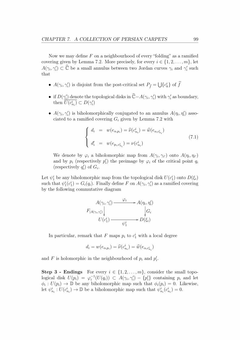
CHAPTER 7. A COLLECTION OF PERSIAN CARPETS 99
Now we may define F on a neighbourhood of every “folding” as a ramifiedcovering given by Lemma 7.2. More precisely, for every i ∈ 1, 2, . . . ,m, letA(γi, γ
′i) ⊂ C be a small annulus between two Jordan curves γi and γ′i such
that
• A(γi, γ′i) is disjoint from the post-critical set Pf =
⋃cik of f
• ifD(γ′i) denote the topological disks in C−A(γi, γ′i) with γ′i as boundary,
then U(cini) ⊂ D(γ′i)
• A(γi, γ′i) is biholomorphically conjugated to an annulus A(ηi, η
′i) asso-
ciated to a ramified covering Gi given by Lemma 7.2 withdi = w(eα,pi) = ν(cini) = w(eα,cini
)
d′i = w(epi,cini) = ν(cini)
(7.1)
We denote by ϕi a biholomorphic map from A(γi, γi′) onto A(ηi, ηi′)and by pi (respectively p′i) the preimage by ϕi of the critical point qi(respectively q′i) of Gi.
Let ψi1 be any biholomorphic map from the topological disk U(ci1) onto D(ξi)such that ψi1(ci1) = Gi(qi). Finally define F on A(γi, γ
′i) as a ramified covering
by the following commutative diagram
A(γi, γ′i)
ϕi //
F|A(γi,γ′i)
A(ηi, η′i)
Gi
U(ci1)ψi1
// D(ξi)
In particular, remark that F maps pi to ci1 with a local degree
di = w(eα,pi) = ν(cini) = w(eα,cini)
and F is holomorphic in the neighbourhood of pi and p′i.
Step 3 - Endings For every i ∈ 1, 2, . . . ,m, consider the small topo-logical disk U(pi) = ϕ−1
i (U(qi)) ⊂ A(γi, γ′i) − p′i containing pi and let
φi : U(pi) → D be any biholomorphic map such that φi(pi) = 0. Likewise,let ψini : U(cini)→ D be a biholomorphic map such that ψini(c
ini
) = 0.

100 CHAPTER 7. A COLLECTION OF PERSIAN CARPETS
Then define F on U(cini) by the following commutative diagram
U(cini)ψini //
F|U(cini )
D
z 7→ zd′i
U(pi)
φi // D
In particular, remark that F maps cini to pi with a local degree
d′i = w(epi,cini) = ν(cini)
Step 4 - Extension Observe that we may easily improve Step 1 and Step 3in order to extend F to the complement of a neighbourhood of
⋃A(γi, γ′i). It
remains to define F on small annuli of the form A(βi, γi) and A(γ′i, β′i) where
i ∈ 1, 2, . . . ,m and βi, β′i are two Jordan curves. The equalities (7.1) implythat
deg(F|βi) = ν(cini) = di = deg(F|γi)
deg(F|γ′i) = d′i = deg(F|β′i)
Therefore F may be extended onto every A(βi, γi) and every A(γ′i, β′i) as a
ramified covering without extra critical point.To sum up, we finally obtain a ramified covering F : C→ C such that• F is holomorphic on
U =
⋃i∈1,2,...,N+1k∈1,2,...,ni
U(cik)
∪ ⋃i∈1,2,...,m
U(pi) ∪ U(p′i)
• the closure of the post-critical set of F is
PF =
⋃i∈1,2,...,N+1k∈1,2,...,ni
cik
∪ ⋃i∈1,2,...,m
pi
∪
⋃i∈1,2,...,m
F n(p′i) / n > 1
• PF ⊂ U
The third point follows from the construction since the forward orbitof each critical point p′i where i ∈ 1, 2, . . . ,m accumulates the super-attracting periodic cycle pi, ci1, pi2, . . . , pini .

CHAPTER 7. A COLLECTION OF PERSIAN CARPETS 101
Step 5- A powerful theorem We are going to conclude the construction(that is to get a rational map f from the ramified covering F ) by using aThurston-like characterization which generalizes Theorem 5.9 for a larger setof ramified coverings which contains F . We follow the notations from [CT07].
Definition 7.3 (sub-hyperbolic semi-rational map). Let F : C → C be anorientation-preserving ramified covering. Denote by P ′F the accumulation setof its post-critical set. We say that F is a sub-hyperbolic semi-rationalmap if the following conditions hold
(i) P ′F is finite
(ii) F is holomorphic in a neighbourhood of P ′F
(iii) every periodic points in P ′F are either attracting or super-attracting
Definition 7.4 (combinatorially equivalence). Two sub-hyperbolic semi-rationalmaps F and G are said combinatorially equivalent if there exist twoorientation-preserving homeomorphisms ϕ0 and ϕ1 of C such that
(i) the following diagram commutes
Cϕ1 //
F
C
GC
ϕ0 // C
(ii) ϕ0(PF ) = ϕ1(PF ) = PG
(iii) ϕ0 is isotopic to ϕ1 relative to PF
(iv) ϕ0 is holomorphic on a neighbourhood of P ′FCompare the definition above with Definition 5.2. Notice that ϕ0 and ϕ1
are actually equal on a neighbourhood of P ′F (by the isolated zero theorem)and then realize a local conformal conjugacy.
The Thurston-like characterization for sub-hyperbolic semi-rational mapis the following.
Theorem 7.5 (Cui Guizhen-Tan Lei). A sub-hyperbolic semi-rational mapF with P ′F 6= ∅ is combinatorially equivalent to a rational map if and only ifit has no Thurston obstruction. In that case, the rational map is unique upto conjugation by a Möbius transformation.
Compare this result with Theorem 5.9. We refer the readers to [CT07]for a proof.
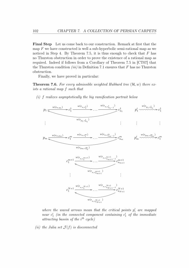
102 CHAPTER 7. A COLLECTION OF PERSIAN CARPETS
Final Step Let us come back to our construction. Remark at first that themap F we have constructed is well a sub-hyperbolic semi-rational map as wenoticed in Step 4. By Theorem 7.5, it is thus enough to check that F hasno Thurston obstruction in order to prove the existence of a rational map asrequired. Indeed if follows from a Corollary of Theorem 7.5 in [CT07] thatthe Thurston condition (iii) in Definition 7.1 ensures that F has no Thurstonobstruction.
Finally, we have proved in particular:
Theorem 7.6. For every admissible weighted Hubbard tree (H, w) there ex-ists a rational map f such that
(i) f realizes asymptotically the big ramification portrait below
p1
w(eα,p1 )// c1
1
w(eα,c11
)// . . .
w(eα,c1n1−1
)
// c1n1
w(ep1,c
1n1
)
ii p′1
w(ep1,c
1n1
)// c1
1
......
......
pmw(eα,pm ) // cm1
w(eα,cm1)// . . .
w(eα,cmnm−1)// cmnm
w(epm,cmn1)
ii p′mw(epm,cmnm
)// cm1
cm+11
w(eα,cm+1
1)// . . .
w(eα,cm+1
nm+1−1)
// cm+1nm+1
w(eα,cm+1
nm+1)
gg
......
cN+11
w(eα,cN+1
1)
// . . .
w(eα,cN+1
nN+1−1)
// cN+1nN+1
w(eα,cN+1
nN+1
)
gg
where the waved arrows mean that the critical points p′i are mappednear ci1 (in the connected component containing ci1 of the immediateattracting bassin of the ith cycle)
(ii) the Julia set J (f) is disconnected

CHAPTER 7. A COLLECTION OF PERSIAN CARPETS 103
7.2 Mandelbrotesque carpetsConsider the abstract Hubbard tree H = (T, τ, δ) displayed in Figure 7.2.
Figure 7.2: The abstract Hubbard tree H
It has one fixed branching point α of Misiurewicz type and two periodiccycle of vertices: one fixed end c0 and one periodic cycle c′0, c′1 of periodtwo containing a critical point c′0. We have
τ(eα,c0) = eα,c0τ(eα,c′0) = eα,c′0 ∪ ec′0,c′1τ(ec′0,c′1) = ec′0,c′1
Equip H with a weight function w. Using the same order for the edgesof H as above, we get the following transition matrix of (H, w)
M =
w(eα,c0)−1 0 0
0 w(eα,c′0)−1 w(eα,c′0)
−1
0 0 w(ec′0,c′1)−1
In particular λ(H) is the largest reciprocal of the weights. Therefore theweighted Hubbard tree (H, w) is unobstructed if and only if every weight isat least two.
For instance consider the weight function w which is equal to two on eachedge. Then the weighted Hubbard tree (H, w) is admissible and consequentlythere exist a rational map hp depending on the parameter p ∈ C realizingasymptotically the ramification portrait below.
0 2ee 1 4 //∞2
aa p2 //∞

104 CHAPTER 7. A COLLECTION OF PERSIAN CARPETS
The last arrow means that the critical point p is mapped in the connectedcomponent containing ∞ of the immediate attracting bassin of hp. Remarkthat hp has three critical points of multiplicity one and one critical pointof multiplicity three, so deg(hp) = 4 (by Riemann-Hurwitz formula). Inparticular hp is of the form
hp : z 7→ az4 + bz3 + cz2 + dz + e
Az4 +Bz3 + Cz2 +Dz + E
Since 1 is mapped to∞ with a local degree four, the denominator may factoras
hp : z 7→ az4 + bz3 + cz2 + dz + e
(z − 1)4
In particular
hp :1
z7→ (a− 1) + (b+ 4)z + (c− 6)z2 + (d+ 4)z3 + ez4
(1− z)4+ 1
Since ∞ is mapped to 1 with a local degree two, it follows a = 1 and b = −4
hp : z 7→ z4 − 4z3 + cz2 + dz + e
(z − 1)4
An easy computation gives the derivative function of hp
f ′p : z 7→ −2(c− 6)z2 + (2c+ 3d)z + (d+ 4e)
(z − 1)5
Since 0 and p are critical points of hp we get the following two equationsd+ 4e = 0
− 2c+ 3d
2(c− 6)= p
⇒
d = −4e
c =12p− 3d
2p+ 2= 6
(p+ e
p+ 1
)
hp : z 7→z4 − 4z3 + 6
(p+ep+1
)z2 − 4ez + e
(z − 1)4(7.2)
It remains the information hp(0) = 0 which lead to e = 0
hp : z 7→z2[z2 − 4z + 6
(pp+1
)](z − 1)4

CHAPTER 7. A COLLECTION OF PERSIAN CARPETS 105
We know that there exist some choices of p (in order to make hp(p) closeto ∞) such that hp is encoded by the weighted Hubbard tree (H, w). Indeedfor p ≈ −1 we get the bifurcation locus in Figure 7.3. Picking a parameter pinside the big hyperbolic component, we obtain the Julia set J (hp) in Figure7.4.
Observe that every Julia component of J (hp) is a point or a Jordan curve(by the result of Tan Lei and K. Pilgrim, see Theorem 6.14).
Figure 7.3: The hyperbolic component of the family (hp)p∈Cinside a disk of center −1 and radius 0.15
Figure 7.4: A Persian carpet with a disk motif

106 CHAPTER 7. A COLLECTION OF PERSIAN CARPETS
Now fixing such a value for the critical point p, we may vary the image ofthe critical point 0 in order that 0 is no longer fixed. Denote by e the imageof 0. The asymptotic ramification portrait is now
0 2 // e 1 4 //∞2
aa p2 //∞
Actually we have already computed an algebraic formula for the rational maphe seen now as depending on the parameter e ∈ C (see (7.2)):
he : z 7→z4 − 4z3 + 6
(p+ep+1
)z2 − 4ez + e
(z − 1)4
For e ≈ 0 we get the bifurcation locus in Figure 7.5. The big hyperboliccomponent containing the parameter e = 0 is the main cardioid of a copyof the Mandelbrot set. Then this copy provides several different kind ofrational maps with disconnected Julia sets, encoded by different admissibleweighted Hubbard tree (see Figure 7.6 and Figure 7.7). Actually we mayfind parameter such that the associated rational map is still “encoded” by aweighted Hubbard tree which is no longer admissible (see Figure 7.8).
Figure 7.5: The hyperbolic component of the family (he)e∈C (p = −1.001)inside a disk of center 0 and radius 0.0005

CHAPTER 7. A COLLECTION OF PERSIAN CARPETS 107
Figure 7.6: A Persian carpet with a rabbit motif
Figure 7.7: Another Persian carpet with a quadratic motif(compare with Figure 6.3)
Figure 7.8: A Persian carpet with a dendrite motif

Chapter 8
Concluding remarks: future works
Theorem 6.18 gives a conjugacy of the rational map f on a subset JH(f) ofJulia components. But it seems that the induced continuous and surjectivemap, say π, from
⋃J∈JH(f) J onto the Hubbard tree H may be continuously
extended to the whole Riemann sphere C (compare with the map π definedin Section 6.2). Unfortunatly, it is difficult to define precisely π on each piececonstructed in Section 6.2, especially on D′3,2 and D(δ′+3,−3) which containssome Julia components as we explained in Section 6.5. Another possible wayto show this is to begin a new construction in a abstract way in order to get asub-hyperbolic semi-rational map which is already “encoded” by the weightedHubbard tree (H, w). Nevertheless, Theorem 7.5 provides only a combinato-rially equivalence, not a topological equivalence as required. Therefore thatwill remain some works to conclude. This issue is linked to a question occur-ring naturally at the end of Chapter 7: how to encode precisely the dynamicsof the constructed rational maps by the weighted Hubbard tree behind ?
We have also to generalize the construction from Chapter 7 to more com-plicated tree than those of Definition 7.1. More precisely, we may at first tryto enlarge the realization condition (ii) by extending Theorem 5.21. To doso, we have to generalize Theorem 4.12 as we already discussed in Section4.3 (topological part) and to consider only the ramified coverings withoutThurston obstruction (analytical part). Such a generalization seems reason-able and it is suggested by Figure 7.8. We may also try to enlarge the treeshape condition (i). That would be done by using Theorem 7.5 in a moregeneral situation.

CHAPTER 8. CONCLUDING REMARKS: FUTURE WORKS 109
Furthermore several question occurs naturally in the way of studying thedynamics of rational maps with disconnected Julia set. In order to know howmuch of dynamical informations is captured by the weighted Hubbard tree,here is a list of issues:
• What about the unicity ? More precisely, if two rational maps areencoded by a same weighted Hubbard tree, are they quasiconformallyconjugated ?
• What about the converse problem ? If a rational map has a discon-nected Julia set, is it always possible to find a weighted Hubbard treestructure behind ?
The second guess seems to be true at least for sub-hyperbolic semi-rationalmap.

Appendix A
Topological tools
This appendix gathers all the topological facts required.
A.1 Plane Topology
We would like to prove two lemmas which were used several times in thisthesis. As many other results in plane topology, both are consequence of thepowerful Jordan’s theorem. We will also recall some classical definitions andresults.
Definition A.1 (Jordan arc and Jordan curve). Let X be a topologicalspace. A Jordan arc between two points a, b ∈ X is the image of the unitsegment [0, 1] by a homeomorphism ` : [0, 1] → X such that `(0) = a and`(1) = b. A Jordan curve in X is the image of the unit circle S1 by ahomeomorphism γ : S1 → X. We will write only ` (respectively γ) to denotea Jordan arc (respectively a Jordan curve) when there is no ambiguity.
Theorem A.2 (Jordan’s curve theorem). The complement of any Jordancurve γ in S2 consists of two distinct connected components and γ is theboundary of each component.
There exist several proofs of this fundamental result in plane topology(using complex analysis, or Brouwer’s fixed point theorem, or graph the-ory,...). The following classical sharpening discuss the topological nature ofconnected components in the complement of a Jordan curve.
Theorem A.3 (Schönflies’ theorem). Let γ : S1 → S2 be a Jordan curvein S2 and denote by D a connected component of S2 − γ. Then there is ahomeomorphism γ : D→ D which extends γ on the whole unit disk.

APPENDIX A. TOPOLOGICAL TOOLS 111
Lemma A.4. Fix a point ω in S2. Let γ (respectively γ′) be a Jordan curvein S2 and denote by D (respectively by D′) the connected component of S2−γ(respectively S2 − γ′) which does not contain ω. Then
γ ∩ γ′ = ∅D ∩D′ 6= ∅ ⇒ D ⊂ D′ or D′ ⊂ D
Proof of Lemma A.4. Let x be in the intersection D ∩ D′. Since γ is con-nected and disjoint from γ′, the Jordan’s curve theorem applied to γ′ implieseither γ ⊂ D′ or γ ⊂ S2 − D′. In the second case, we get γ ∩ D′ = ∅ andthen the connected set D′ is necessarily in the connected component of S2−γwhich contains x, that is D′ ⊂ D. So we may assume γ ⊂ D′ and γ′ ⊂ Dby symmetry. In particular γ and γ′ are not contained in the boundary ofD ∪D′. Furthermore this boundary is contained in ∂D ∪ ∂D′ which is equalto γ ∪ γ′ by the Jordan’s curve theorem. Finally D ∪ D′ = S2, that is acontradiction with the existence of the point ω.
Definition A.5 (homotopic Jordan curves). Let P ⊂ S2 be a finite set. TwoJordan curves γ0 and γ1 in S2 − P are said homotopic in S2 − P if thereexists a homotopy ϕ : [0, 1]× S1 → S2 − P, (t, .) 7→ ϕ(t, .) from ϕ(0,S1) = γ0
to ϕ(1,S1) = γ1 where ϕ(0, .) and ϕ(1, .) are homeomorphisms.
Notice that the distinction between a homeomorphism and its image todefine a Jordan curve is important in definition above. For instance, thehomeomorphisms e2iπθ 7→ e2iπθ and e2iπθ 7→ e−2iπθ are not homotopic inC−0,∞ (with identification of S2 and C as topologic manifolds) but theydefine the same Jordan curve.
Lemma A.6. Let P be a subset of S2. Let γ (respectively γ′) be a Jordancurve in S2 − P and let D (respectively D′) be a connected component ofS2−γ (respectively S2−γ′). If γ and γ′ are homotopic in S2−P then D∩Pis equal to either D′ ∩ P or (S2 −D′) ∩ P .
In order to prove the lemma above, we will need the following useful tool.
Definition A.7 (winding number). Let φ : S1 → C be a continuous functionand a be a point in C − φ(S1). We can rewrite φ : e2iπt 7→ a + r(t)e2iπθ(t)
where r : [0, 1] →]0,+∞[ and θ : [0, 1] → R are required to be continuous.The winding number of φ around a, denoted by Indφ(a), is the integer
Indφ(a) = θ(1)− θ(0)
and it does not depend on choice of continuous function θ : [0, 1]→ R.

112 APPENDIX A. TOPOLOGICAL TOOLS
Recall some results about the winding number.
Proposition A.8. We have the following properties.
1. The winding number is continuous: for every continuous function φ :S1 → C, Indφ is constant on each connected component of C− φ(S1).
2. The winding number is constant on the homotopy classes: for everycontinuous functions φ0, φ1 : S1 → C, and every point a ∈ C−(φ0(S1)∪φ1(S1)), if there exists a homotopy ϕ : [0, 1] × S1 → C − a, (t, .) 7→ϕ(t, .) from ϕ(0, .) = φ0 to ϕ(1, .) = φ1 then Indφ0(a) = Indφ1(a).
3. The winding number of a Jordan curve γ on C is equal to 1 or -1 onthe bounded connected component of C − γ and 0 on the unboundedconnected component.
Let us come back to the Lemma A.6.
Proof of Lemma A.6. We may assume that P 6= ∅ and, by Jordan’s curvetheorem, (S2−D)∩(S2−D′)∩P 6= ∅ (exchanging D with S2−D and D′ withS2−D′ if necessary). We have thus to prove that D∩P = D′∩P . Let ω be apoint in the intersection (S2−D)∩(S2−D′)∩P and identify S2−ω with Cas topological manifolds. Now compare Indγ and Indγ′ at every point a ∈ P−ω. Since γ and γ′ are homotopic in S2 − a, if follows Indγ(a) = Indγ′(a)from the second point of Proposition A.8. Moreover Indγ(a) (respectivelyIndγ′(a)) is not equal to 0 if and only if a ∈ D (respectively a ∈ D′) by thethird point of Proposition A.8. The conclusion follows.
A.2 Ramified coveringsWe would like to recall the definition of ramified coverings together with someclassical results. We refer the readers to [Dou05] for deeper discussions.
Definition A.9 (ramified covering). Let U1 and U2 be two toplogical mani-folds of real dimension two (not necessarily equipped with a Riemann surfacestructure). A continuous function f : U1 → U2 is a ramified covering if forevery y ∈ U2 there exists a connected neighbourhood D(y) such that
• f−1(D(y)) is a nonempty union (possibly finite) of pairwise disjointsconnected open sets
f−1(D(y)) =⋃k>1
B(xk)

APPENDIX A. TOPOLOGICAL TOOLS 113
• for every integer k > 1, there exist a positive integer dk > 1 and twocharts (i.e. homeomorphisms) ϕk : B(xk)→ D and ϕ : D(y)→ D suchthat ϕk(xk) = 0, ϕ(y) = 0 and the following diagram commutes
B(xk)ϕk //
f
D
z 7→ zdk
D(y)ϕ // D
The integer dk is called the local degree of f at xk and it is denoted bydegloc(f)(xk). Furthermore if degloc(f)(xk) > 1, we say that xk is a criti-cal point of f of multiplicity degloc(f)(xk) − 1. Finally an unbranchedcovering is a ramified covering without critical point.
Definition A.10 (orientation-preserving ramified covering). Let f : U1 →U2 be a ramified covering between two orientable topological manifolds ofreal dimension two. f is said orientation-preserving if for every pair ofcharts ϕ1 : V1 → D and ϕ2 : V2 → D in Definition A.9 where V1 ∩ V2 isnonempty, the transition map
ϕ1,2 = (ϕ2 ϕ−11 )|ϕ1(V1∩V2) : ϕ1(V1 ∩ V2)→ ϕ2(V1 ∩ V2)
is orientation-preserving (where D ⊂ C comes with the usual counterclock-wise orientation).
Proposition A.11. Let f : U1 → U2 be a ramified covering between twotopological manifolds of real dimension two. The following holds.
1. The critical points of f are isolated points in U1.
2. There exists d ∈ N ∪ ∞, called the degree of f , such that
∀y ∈ U2,∑x∈U1f(x)=y
degloc(f)(x) = d
In particular f is a surjective map.
3. For every connected open set V2 ⊂ U2 and every V1 connected compo-nent of f−1(V2), f|V1 : V1 → V2 is a ramified covering.
4. In case d <∞, for every connected compact set K2 ⊂ U2 and every K1
connected component of f−1(K2), f(K1) = K2.

114 APPENDIX A. TOPOLOGICAL TOOLS
The following powerful result makes a link between ramification and al-gebraic topology.
Theorem A.12 (Riemann-Hurwitz formula). Let V1 and V2 be two connectedopen sets in S2. Denote by m1 (respectively m2) the number of connectedcomponents in S2 − V1 (respectively S2 − U2). If f : U1 → U2 is a ramifiedcovering of degree d ∈ N then
m1 − 2 = d(m2 − 2) + r where r =∑x∈V1
(degloc(f)(x)− 1)
As a consequence, a rational map R : C→ C of degree d > 1 has exactly2d− 2 critical points counted with multiplicity.

Appendix B
Linear algebra
We would like to recall in this appendix some classical definitions and resultsin linear algebra, notably the Perron-Frobenius theorem. All these resultsare needed in the discussion around the Thurston’s theorem (Chapter 5).We will not give proofs, except for the last corollary which justifies crucialDefinition 5.8 and Definition 6.10.
Definition B.1 (spectral radius). The spectral radius of a matrix M ∈Mn(C), denoted by ρ(M) is the largest modulus of its eigenvalues.
ρ(M) = max|λ| / λ ∈ Sp(M)
In other words, the spectral radius is the largest modulus of roots of thecharacteristic polynomial: χM(X) = det(M −XIn) ∈ Cn[X]. From the factthat polynomial roots depend continuously on coefficients, we get:
Proposition B.2. For any matrix norm ‖.‖ onMn(C), the spectral radiusis a continuous function from (Mn(C), ‖.‖) to (R, |.|).
Theorem B.3 (Gelfand’s formula). For any matrix norm ‖.‖ on Mn(C),we have:
∀M ∈Mn(C), ρ(M) = limk→∞‖Mk‖
1k
Definition B.4 (positive or non-negative matrices). A matrix is said pos-itive, respectively non-negative, if all its coefficients are positive, respec-tively non-negative. For two matrices A,B ∈Mn(C) we write A 6 B if thematrix B − A is non-negative.
Proposition B.5. The spectral radius is increasing on the set of non-negativematrices.
∀A,B ∈Mn(R+), A 6 B ⇒ ρ(A) 6 ρ(B)

116 APPENDIX B. LINEAR ALGEBRA
Proposition B.6. Let M ∈Mn(R+) be a non-negative matrix. The spectralradius of any square sub-block Mi,j ∈Mk(R+) is less than the spectral radiusof M .
ρ(Mi,j) 6 ρ(M) where M =
∗ ∗ ∗∗ Mi,j ∗∗ ∗ ∗
Theorem B.7 (Perron-Frobenius theorem). Let M be a positive matrix.Then ρ(M) is an eigenvalue of M and it is the only one with the largestmodulus. Moreover there exists an associated eigenvector with positive en-tries.
Corollary B.8. Let M be a non-negative matrix. Then ρ(M) is an eigen-value of M . Moreover for every ε > 0 there exists a vector y with positiveentries such that My 6 (ρ(M) + ε)y.
Proof of Corollary B.8. Denote by (mi,j) the entries of M . For every integerk > 1, letMk be the positive matrix of coefficients (mi,j + 1
k). By the Perron-
Frobenius theorem, there exists a positive eigenvector vk associated to theeigenvalue ρ(Mk). Denote by xk = vk
‖vk‖the normalized vector for any vector
norm ‖.‖ on Rn. Since the set S = x ∈ Rn / ‖x‖ = 1 is compact, we canextract a sub-sequence (xϕ(k)) which tends to a non-negative vector x ∈ S.Moreover limk→∞Mk = M and limk→∞ ρ(Mk) = ρ(M) because of continuityof spectral radius (Proposition B.2). Finally we get
Mx = limk→∞
Mϕ(k)xϕ(k) = limk→∞
ρ(Mϕ(k))xϕ(k) = ρ(M)x
Now let k > 1 be large enough such that the inequality ρ(Mϕ(k)) 6 ρ(M) + εholds. The result follows with y = xϕ(x).

Appendix C
Complex analysis
This last appendix gathers some classical results in complex analysis whichwere often used in this thesis.
C.1 Riemann’s mapping theoremTheorem C.1 (Riemann’s mapping theorem). If U is a topological disk inthe Riemann sphere, that is a nonempty simply connected open subset of Cwhose complement contains at least two points, then there exists a biholo-morphic map ϕ : D→ U from the unit disk onto U .
We refer the readers to [Ahl79] or any other lecture about complex anal-ysis for a proof. Notice that up to precomposition by an automorphism ofD, that is a map of the form
D→ D, z 7→ eiθz − a
1− |a|zwhere eiθ ∈ ∂D and a ∈ D
we may always prescribe the image of 0 and the argument of ϕ′(0) (actuallythe map ϕ is unique for given (ϕ(0), ϕ
′(0)|ϕ′(0)|) ∈ U × ∂D).
This powerful result has several consequences in many fields of mathe-matics. In particular it provides a classification of all the simply connectedopen subsets of C (and likewise for any Riemann surface). There are somekinds of generalization. We are going to present two of them. At first thequestion of extension on the boundary of the unit disk as in the followingresult.
Theorem C.2 (Carathéodory’s theorem). Let U be a topological disk in Cwith a locally connected boundary ∂U . Then any biholomorphic map ϕ : D→U extends continuously to the unit circle: ϕ : D→ U .
118 APPENDIX C. COMPLEX ANALYSIS
Secondly consider the same problem for doubly connected domains. Wehave the following classical results.
Theorem C.3. Let U be a topological disk in C and let K be a connected andrelatively compact subset of U which contains at least two points. Then thereexists a unique r ∈]0, 1[ such that U −K is biholomorphically conjugated tothe annulus z ∈ C / r < |z| < 1.
That justifies the following definition.
Definition C.4 (modulus of annulus). Let γ and γ′ be two disjoint continuain the Riemann sphere, that is two nonempty compact connected subsetsof C. We denote by A(γ, γ′) the unique doubly connected component ofC − (γ ∪ γ′). The modulus of the annulus A(γ, γ′) is the unique positivenumber mod(γ, γ′)> 0 such that A(γ, γ′) is biholomorphically conjugatedto the annulus
z ∈ C / r < |z| < 1 where r = e−2πmod(γ,γ′) ⇔ mod(γ, γ′) =1
2πlog
(1
r
)By extension we write mod(A) for every annulus A.
Proposition C.5. Let f : A1 → A2 be a conformal map of degree d > 1between two annuli A1, A2 ⊂ C. Then
mod(A1) =1
dmod(A2)
Theorem C.6 (Grötzsch’s inequality). Let A ⊂ C be an annulus and A1, A2 ⊂A be two disjoint annulli such that the two connected components of theboundary of A are neither in the same connected component of C − A1 norin the same connected component of C− A2. Then
mod(A1) + mod(A2) 6 mod(A)
The following useful result is due to Cui Guizhen and Tan Lei. Anequipotential in a topological disk U ⊂ C is the image of a round circlez ∈ D / |z| = r where r ∈]0, 1[ by any biholomorphic map ϕ : D→ U .
Lemma C.7 (Inverse Grötzsch’s inequality). Let U1 and U2 be two disjointtopological disks in C whose boundary are respectively denoted by α1 andα2. Then there exists a positive constant C > 0 such that for every pair ofequipotentials γ1 ⊂ U1 and γ2 ⊂ U2 the following inequalities hold
mod(α1, γ1) + mod(α2, γ2) 6 mod(γ1, γ2) 6 mod(α1, γ1) + mod(α2, γ2) + C
The left hand side is the classical Grötzsch’s inequality. The right handside is a consequence of Koebe 1/4-theorem. We refer the readers to [CT07]for a complete proof.
APPENDIX C. COMPLEX ANALYSIS 119
C.2 Quasiconformal surgeryA. Douady, J. H. Hubbard and D. Sullivan were the first to understand thepower of quasiconformal maps in holomorphic dynamical systems. Thesemaps allowed in particular to prove the Sullivan’s non-wandering domainstheorem or the sharpest value of the number of non-repelling cycles by M.Shishikura. It is now a standard tool. We would like to present a briefoverview of this theory, especially the quasiconformal surgery method. Thereaders are refered to [Ahl06] for more overall presentation of quasiconformalmaps and to [Bea91], [CG93] or [BM01] for proofs of classical results inholomorphic dynamical systems using the quasiconformal surgery method.
If a map ϕ : C → C is differentiable, we denote by ϕx and ϕy its partialderivatives and we use the following standard differential operators:
ϕz = 12(ϕx − iϕy)
ϕz = 12(ϕx + iϕy)
Observe that if ϕ is holomorphic thenϕz = ϕ′(z)ϕz = 0
The generalization of these equations is the Beltrami equation:
ϕz = µ(z)ϕz (C.1)
where µ is some suitable complex function.
Definition C.8 (almost complex structure). Let U be a domain in the Rie-mann sphere, that is a nonempty open connected subset of C. An almostcomplex structure on U is a Lebesgue measurable function µ: U → C suchthat ‖µ‖∞ < 1.
Definition C.9 (quasiconformal map). Let U be a domain in C. A home-omorphism ϕ : U → C is a quasiconformal map if ϕ is a solution of theBeltrami equation (C.1) for an almost complex structure µ on U , called thedilatation or the Beltrami coefficient of ϕ. Moreover if
‖µ‖∞ 6 k < 1
then ϕ is said to be a k-quasiconformal map.
If ϕ is differentiable at z ∈ U , the preimage of a circle by the differentialdϕ(z) = ϕzdz + ϕzdz is an ellipse whose the argument of the major axis is

120 APPENDIX C. COMPLEX ANALYSIS
12(π+ arg(µ)) and the ratio of major to minor axis is 1+|µ|
1−|µ| . So the dilatationµ of a quasiconformal map ϕ may be seen as an infinitesimal ellipse field.Moreover ϕ is k-quasiconformal means that the “stretching” (i.e. the ratio ofmajor to minor axis of infinitesimal ellipse) of ϕ is uniformally bounded:
1 61 + |µ|1− |µ|
61 + k
1− k
The following result provides a positive answer for the question of theexistence of solutions for Beltrami equation (C.1).
Theorem C.10 (measurable Riemann’s mapping theorem). Let µ be analmost complex structure on a domain U in C. Then there exists a quasicon-formal map ϕ : U → C with dilatation µ.
Moreover it is shown that there is uniqueness up to postcomposing bya biholomorphic map. Notice that for U simply connected (whose comple-ment contains at least two points) and µ identically zero we get the classicalRiemann’s mapping theorem (see Theorem C.1).
Definition C.11 (quasiregular map). Let U be a domain in C. A mapF : U → C is said quasiregular on V ⊂ U if for every z ∈ V , F isholomorphic or quasiconformal on a neighbourhood of z.
Notice that if F is quasiregular on a compact set K then there existsa positive number k < 1 such that for every z ∈ K, F is holomorphic ork-quasiconformal on a neighbourhood of z.
Proposition C.12. Let U be a domain in C and let K be a connected andrelatively compact subset of U whose boundary is the union of a finite numberof disjoint smooth curves (i.e. the image of the unit circle S1 by a diffeomor-phism). Let f : U −K → C be a holomorphic map which extends diffeomor-phically to the boundary ∂K. Then f extends to U by a quasiregular mapwithout critical points in K.
The proposition above was used in this thesis in order to define piecewiselysome quasiregular maps. That is not the most general statement, but we didnot require more.
The very useful following result was stated by M. Shishikura in [Shi87]and it is the basic principle of the quasiconformal surgery method.

APPENDIX C. COMPLEX ANALYSIS 121
Theorem C.13 (Shishikura’s principle on quasiconformal surgery). Assumethat a map F : C→ C satisfies the following points:
• F|H : H → C is holomorphic on an open set H ⊂ C
• F extends quasiregularly to the complement Q = C−H
• there exists an open set A ⊂ H such that F (A) ⊂ A and
∃N ∈ N /F N(Q) ⊂ A
Then there exists an almost complex structure µ on C which is F -invariant(i.e. such that every infinitesimal ellipse associated to µ at z is mapped bydF (z) to the infinitesimal ellipse associated to µ at F (z) for almost everyz ∈ C).
In particular, if ϕ : C→ C is the quasiconformal map of dilatation µ givenby measurable Riemann’s mapping theorem then the map f = ϕ F ϕ−1 isholomorphic.
The main idea of the proof of this result is to pullback infinite numberof times an infinitesimal circle field by F . Then we get an F -invariant in-finitesimal ellipse field which is well defined since we go only a finite numberof times through Q where the “stretching” of F is uniformally bounded (it isnull elsewhere since F is holomorphic).

Bibliography
[AF00] Lluís Alsedà and Núria Fagella. Dynamics on Hubbard trees. Fun-damenta Mathematicae, 164:115–141, 2000.
[Ahl79] Lars V. Ahlfors. Complex analysis. McGraw-Hill Companies, Inc.,third revised edition, 1979.
[Ahl06] Lars V. Ahlfors. Lectures on quasiconformal mappings, volume 38.American Mathematical Society, second revised edition, 2006.
[Bea91] Alan F. Beardon. Iteration of rational functions, volume 132.Springer-Verlag New York, 1991.
[BFH92] Ben Bielefeld, Yuval Fisher, and John H. Hubbard. The classifi-cation of critically preperiodic polynomials as dynamical systems.Journal of the American Mathematical Society, 5(4):721–762, 1992.
[BH92] Bodil Branner and John H. Hubbard. The iteration of cubic poly-nomials. Part two: Patterns and parapatterns. Acta Mathematica,169(3-4):229–325, 1992.
[BM01] François Berteloot and Volker Mayer. Rudiments de dynamiqueholomorphe, volume 7. Société Mathématique de France, EDPSciences, 2001.
[BN06] Laurent Bartholdi and Volodymyr Nekrashevych. Thurston equiv-alence of topological polynomials. Acta Mathematica, 197(1):1–51,2006.
[CG93] Lennart Carleson and Theodore W. Gamelin. Complex dynamics.Springer-Verlag New York, 1993.
[CPT09] Cui Guizhen, Peng Wenjuan, and Tan Lei. On the topology ofwandering Julia components. preprint, 2009.

BIBLIOGRAPHY 123
[CT07] Cui Guizhen and Tan Lei. A characterization of hyperbolic rationalmaps. arXiv:math/0703380v2 [math.DS], 2007.
[DH84] Adrien Douady and John H. Hubbard. Etude dynamique despolynômes complexes (Première partie). Publications Mathéma-tiques d’Orsay, 1984.
[DH93] Adrien Douady and John H. Hubbard. A proof of Thurston’s topo-logical characterization of rational functions. Acta Mathematica,171(2):263–297, 1993.
[Dou05] Adrien et Régine Douady. Algèbre et théories galoisiennes. Cassini,2005.
[Kam01] Atsushi Kameyama. The Thurston equivalence for postcritically fi-nite branched coverings. Osaka Journal of Mathematics, 38(3):565–610, 2001.
[Koc07] Sarah Koch. La théorie de Teichmüller et ses applications auxendomorphismes de Pn. PhD thesis, Université de Provence, 2007.
[Lev85] Silvio V. F. Levy. Critically finite rational maps. PhD thesis,Princeton University, 1985.
[McM94] Curtis T. McMullen. Complex dynamics and renormalization, vol-ume 135. Princeton University Press, 1994.
[Mil06] John Milnor. Dynamics in one complex variable, volume 160.Princeton University Press, third edition, 2006.
[Pil03] Kevin M. Pilgrim. An algebraic formulation of Thurston’s com-binatorial equivalence. Proceedings of the American MathematicalSociety, 131(11):3527–3534, 2003.
[Poi93] Alfredo Poirier. On post critically finite polynomials. Part two:Hubbard trees. arXiv:math/9307235v1 [math.DS], 1993.
[PT00] Kevin M. Pilgrim and Tan Lei. Rational maps with disconnectedJulia set. Astérisque, 261:349–384, 2000.
[Shi87] Mitsuhiro Shishikura. On the quasiconformal surgery of rationalfunctions. Annales Scientifiques de l’Ecole Normale Supérieure,20:725–752, 1987.

124 BIBLIOGRAPHY
[ST00] Mitsuhiro Shishikura and Tan Lei. A family of cubic rational mapsand matings of cubic polynomials. Experimental Mathematics,9(1):29–53, 2000.
[Tan92] Tan Lei. Matings of quadratic polynomials. Ergodic Theory andDynamical Systems, 12:589–620, 1992.
[Zha08] Zhang Gaofei. Dynamics of Siegel rational maps with prescribedcombinatorics. arXiv:math/08113043v1 [math.DS], 2008.
