goodrich, tamassia search trees1 binary search trees 6 9 2 4 1 8

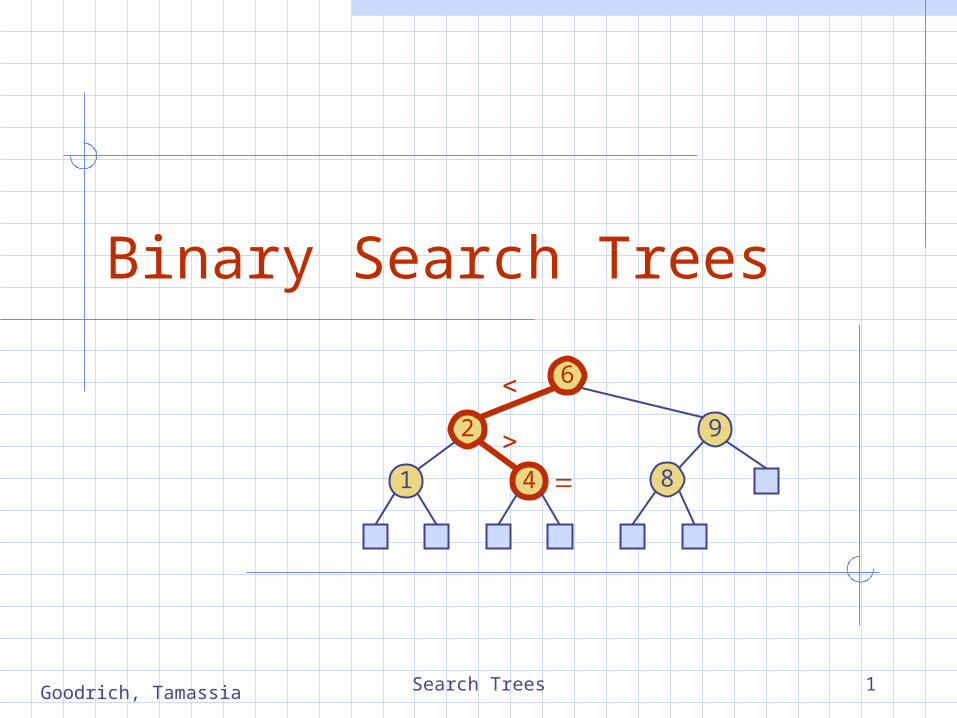
Search Trees 1Goodrich, Tamassia

Binary Search Trees

6

92

41 8


Ordered DictionariesKeys are assumed to come from a total order.New operations: first(): first entry in the dictionary ordering last(): last entry in the dictionary ordering successors(k): iterator of entries with keys

greater than or equal to k; increasing order predecessors(k): iterator of entries with

keys less than or equal to k; decreasing order


Binary Search (§ 8.3.3)Binary search can perform operation find(k) on a dictionary implemented by means of an array-based sequence, sorted by key

similar to the high-low game at each step, the number of candidate items is halved terminates after O(log n) steps

Example: find(7)

1 3 4 5 7 8 9 11 14 16 18 19

1 3 4 5 7 8 9 11 14 16 18 19

1 3 4 5 7 8 9 11 14 16 18 19

1 3 4 5 7 8 9 11 14 16 18 19

0

0

0

0

ml h

ml h

ml h

lm h


Search Tables

A search table is a dictionary implemented by means of a sorted sequence

We store the items of the dictionary in an array-based sequence, sorted by key

We use an external comparator for the keysPerformance:

find takes O(log n) time, using binary search insert takes O(n) time since in the worst case we have to

shift n2 items to make room for the new item remove take O(n) time since in the worst case we have to

shift n2 items to compact the items after the removalThe lookup table is effective only for dictionaries of small size or for dictionaries on which searches are the most common operations, while insertions and removals are rarely performed (e.g., credit card authorizations)


Binary Search Trees (§ 9.1)A binary search tree is a binary tree storing keys (or key-value entries) at its internal nodes and satisfying the following property:

Let u, v, and w be three nodes such that u is in the left subtree of v and w is in the right subtree of v. We have key(u) key(v) key(w)

External nodes do not store items

An inorder traversal of a binary search trees visits the keys in increasing order

6

92

41 8


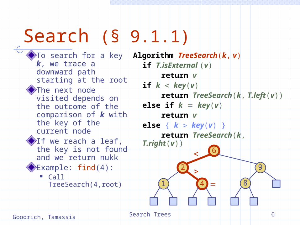
Search (§ 9.1.1)To search for a key k, we trace a downward path starting at the rootThe next node visited depends on the outcome of the comparison of k with the key of the current nodeIf we reach a leaf, the key is not found and we return nukkExample: find(4):

Call TreeSearch(4,root)

Algorithm TreeSearch(k, v)if T.isExternal (v)

return vif k key(v)

return TreeSearch(k, T.left(v))else if k key(v)

return velse { k key(v) }

return TreeSearch(k, T.right(v))

6

92

41 8


InsertionTo perform operation inser(k, o), we search for key k (using TreeSearch)Assume k is not already in the tree, and let let w be the leaf reached by the searchWe insert k at node w and expand w into an internal nodeExample: insert 5

6

92

41 8

6

92

41 8

5

w

w


DeletionTo perform operation remove(k), we search for key kAssume key k is in the tree, and let let v be the node storing kIf node v has a leaf child w, we remove v and w from the tree with operation removeExternal(w), which removes w and its parentExample: remove 4

6

92

41 8

5

vw

6

92

51 8


Deletion (cont.)We consider the case where the key k to be removed is stored at a node v whose children are both internal

we find the internal node w that follows v in an inorder traversal

we copy key(w) into node v we remove node w and its

left child z (which must be a leaf) by means of operation removeExternal(z)

Example: remove 3

3

1

8

6 9

5

v

w

z

2

5

1

8

6 9

v

2


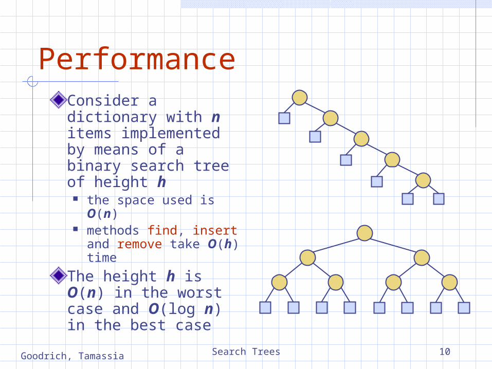
PerformanceConsider a dictionary with n items implemented by means of a binary search tree of height h

the space used is O(n) methods find, insert

and remove take O(h) time

The height h is O(n) in the worst case and O(log n) in the best case


AVL Trees6

3 8

4

v

z


AVL Tree Definition (§ 9.2)

AVL trees are balanced.An AVL Tree is a binary search tree such that for every internal node v of T, the heights of the children of v can differ by at most 1.

88

44

17 78

32 50

48 62

2

4

1

1

2

3

1

1

An example of an AVL tree where the heights are shown next to the nodes:


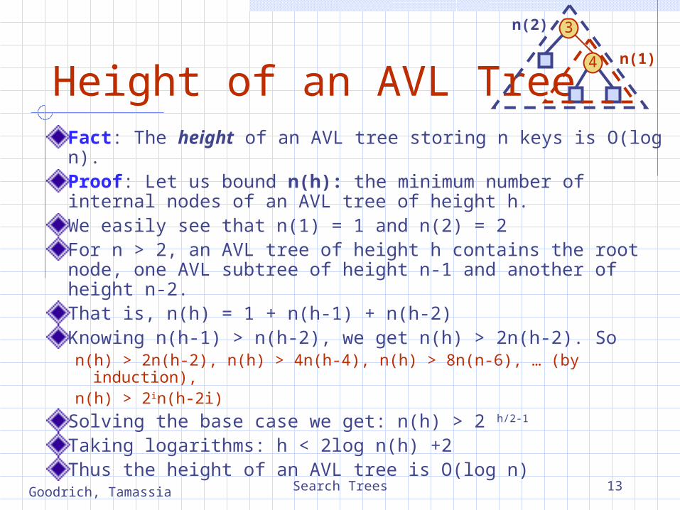
Height of an AVL TreeFact: The height of an AVL tree storing n keys is O(log n).Proof: Let us bound n(h): the minimum number of internal nodes of an AVL tree of height h.We easily see that n(1) = 1 and n(2) = 2For n > 2, an AVL tree of height h contains the root node, one AVL subtree of height n-1 and another of height n-2.That is, n(h) = 1 + n(h-1) + n(h-2)Knowing n(h-1) > n(h-2), we get n(h) > 2n(h-2). Son(h) > 2n(h-2), n(h) > 4n(h-4), n(h) > 8n(n-6), … (by induction),n(h) > 2in(h-2i)

Solving the base case we get: n(h) > 2 h/2-1

Taking logarithms: h < 2log n(h) +2Thus the height of an AVL tree is O(log n)

3

4 n(1)

n(2)


Insertion in an AVL TreeInsertion is as in a binary search treeAlways done by expanding an external node.Example: 44

17 78

32 50 88

48 62

54w

b=x

a=y

c=z

44

17 78

32 50 88

48 62

before insertion after insertion


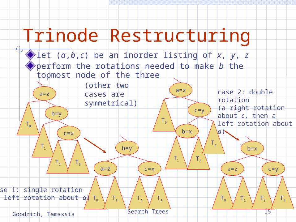
Trinode Restructuringlet (a,b,c) be an inorder listing of x, y, zperform the rotations needed to make b the topmost node of the three

b=y

a=z

c=x

T0

T1

T2 T3

b=y

a=z c=x

T0 T1 T2 T3

c=y

b=x

a=z

T0

T1 T2

T3b=x

c=ya=z

T0 T1 T2 T3

case 1: single rotation(a left rotation about a)

case 2: double rotation(a right rotation about c, then a left rotation about a)

(other two cases are symmetrical)


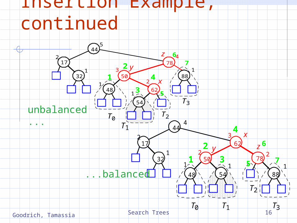
Insertion Example, continued

88

44

17 78

32 50

48 62

2

5

1

1

3

4

2

1

54

1

T0T2

T3

x

y

z

2

3

4

5

67

1

88

44

17

7832 50

48

622

4

1

1

2 2

3

154

1

T0 T1

T2

T3

x

y z

unbalanced...

...balanced

1

2

3

4

5

6

7

T1


Restructuring (as Single Rotations)

Single Rotations:

T0T1

T2

T3

c = xb = y

a = z

T0 T1 T2

T3

c = xb = y

a = zsingle rotation

T3T2

T1

T0

a = xb = y

c = z

T0T1T2

T3

a = xb = y

c = zsingle rotation


Restructuring (as Double Rotations)

double rotations:

double rotationa = z

b = xc = y

T0T2

T1

T3 T0

T2T3T1

a = zb = x

c = y

double rotationc = z

b = xa = y

T0T2

T1

T3 T0

T2T3 T1

c = zb = x

a = y


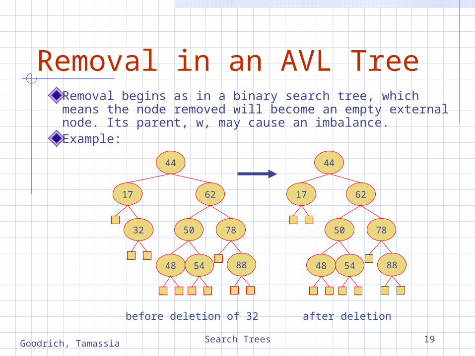
Removal in an AVL TreeRemoval begins as in a binary search tree, which means the node removed will become an empty external node. Its parent, w, may cause an imbalance.Example:

44

17

7832 50

8848

62

54

44

17

7850

8848

62

54

before deletion of 32 after deletion


Rebalancing after a Removal

Let z be the first unbalanced node encountered while travelling up the tree from w. Also, let y be the child of z with the larger height, and let x be the child of y with the larger height.We perform restructure(x) to restore balance at z.As this restructuring may upset the balance of another node higher in the tree, we must continue checking for balance until the root of T is reached44

17

7850

8848

62

54

w

c=x

b=y

a=z

44

17

78

50 88

48

62

54


Running Times for AVL Trees

a single restructure is O(1) using a linked-structure binary tree

find is O(log n) height of tree is O(log n), no restructures needed

insert is O(log n) initial find is O(log n) Restructuring up the tree, maintaining heights is O(log

n)

remove is O(log n) initial find is O(log n) Restructuring up the tree, maintaining heights is O(log

n)


(2,4) Trees

9

10 142 5 7


Multi-Way Search Tree (§ 9.4.1)

A multi-way search tree is an ordered tree such that Each internal node has at least two children and stores d1

key-element items (ki, oi), where d is the number of children For a node with children v1 v2 … vd storing keys k1 k2 … kd1

keys in the subtree of v1 are less than k1

keys in the subtree of vi are between ki1 and ki (i = 2, …, d1) keys in the subtree of vd are greater than kd1

The leaves store no items and serve as placeholders

11 24

2 6 8 15

30

27 32


Multi-Way Inorder Traversal

We can extend the notion of inorder traversal from binary trees to multi-way search treesNamely, we visit item (ki, oi) of node v between the recursive traversals of the subtrees of v rooted at children vi and vi1

An inorder traversal of a multi-way search tree visits the keys in increasing order

11 24

2 6 8 15

30

27 32

1 3 5 7 9 11 13 19

15 17

2 4 6 14 18

8 12

10

16


Multi-Way SearchingSimilar to search in a binary search treeA each internal node with children v1 v2 … vd and keys k1 k2 … kd1

k ki (i = 1, …, d1): the search terminates successfully k k1: we continue the search in child v1

ki1 k ki (i = 2, …, d1): we continue the search in child vi

k kd1: we continue the search in child vd

Reaching an external node terminates the search unsuccessfullyExample: search for 30

11 24

2 6 8 15

30

27 32


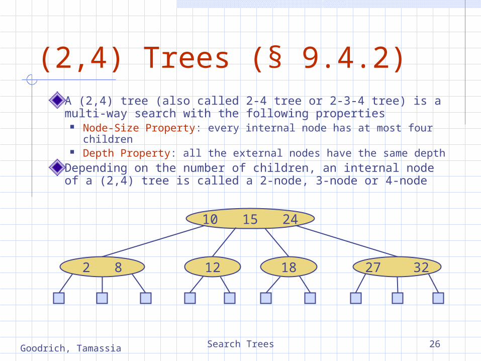
(2,4) Trees (§ 9.4.2)A (2,4) tree (also called 2-4 tree or 2-3-4 tree) is a multi-way search with the following properties

Node-Size Property: every internal node has at most four children

Depth Property: all the external nodes have the same depth

Depending on the number of children, an internal node of a (2,4) tree is called a 2-node, 3-node or 4-node

10 15 24

2 8 12 27 3218


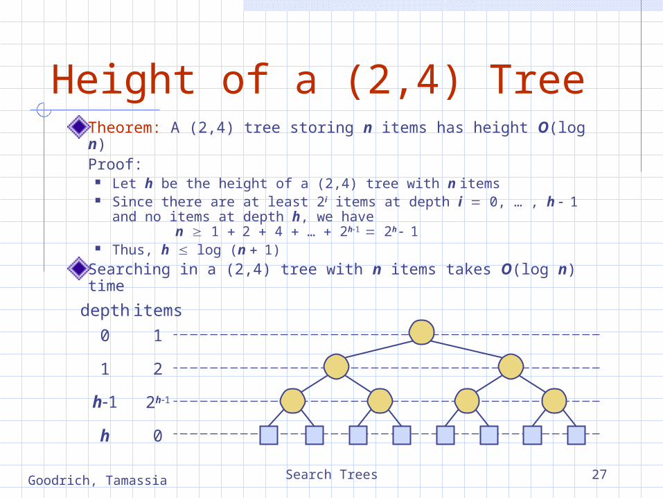
Height of a (2,4) TreeTheorem: A (2,4) tree storing n items has height O(log n)Proof:

Let h be the height of a (2,4) tree with n items Since there are at least 2i items at depth i 0, … , h 1 and

no items at depth h, we have n 1 2 4 … 2h1 2h 1

Thus, h log (n 1)

Searching in a (2,4) tree with n items takes O(log n) time

1

2

2h1

0

items

0

1

h1

h

depth


InsertionWe insert a new item (k, o) at the parent v of the leaf reached by searching for k

We preserve the depth property but We may cause an overflow (i.e., node v may become a 5-node)

Example: inserting key 30 causes an overflow

27 32 35

10 15 24

2 8 12 18

10 15 24

2 8 12 27 30 32 3518

v

v


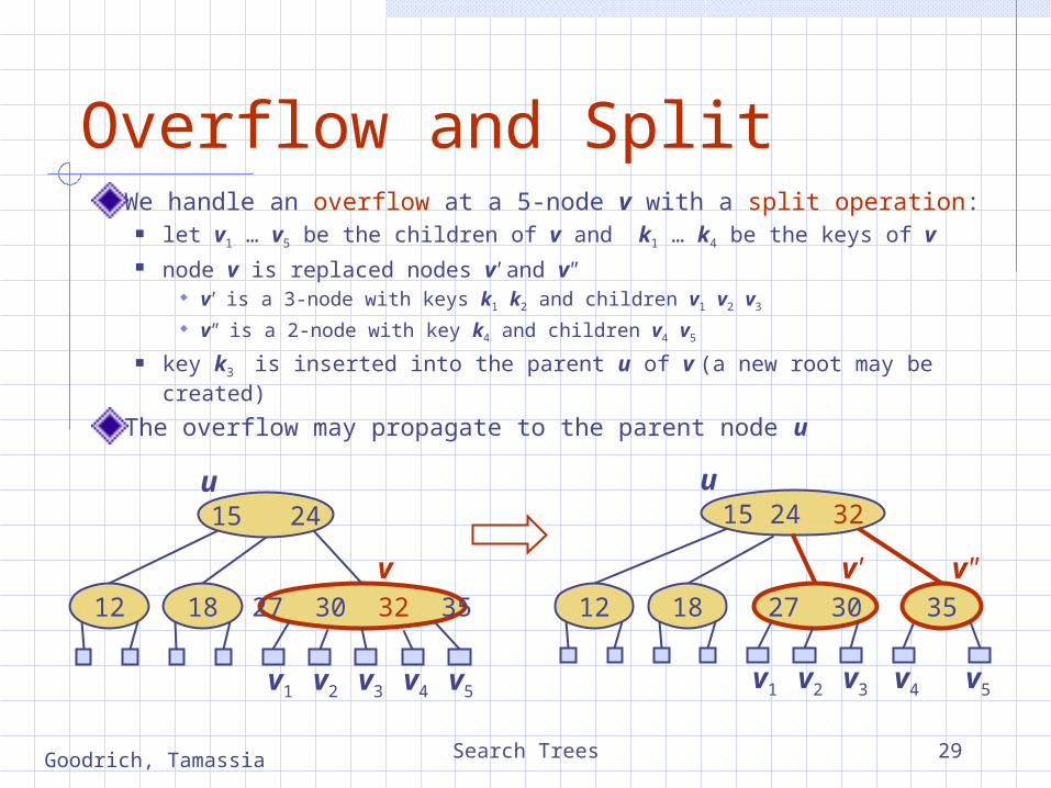
Overflow and SplitWe handle an overflow at a 5-node v with a split operation:

let v1 … v5 be the children of v and k1 … k4 be the keys of v node v is replaced nodes v' and v"

v' is a 3-node with keys k1 k2 and children v1 v2 v3

v" is a 2-node with key k4 and children v4 v5

key k3 is inserted into the parent u of v (a new root may be created)

The overflow may propagate to the parent node u

15 24

12 27 30 32 3518v

u

v1 v2 v3 v4 v5

15 24 32

12 27 3018v'

u

v1 v2 v3 v4 v5

35v"


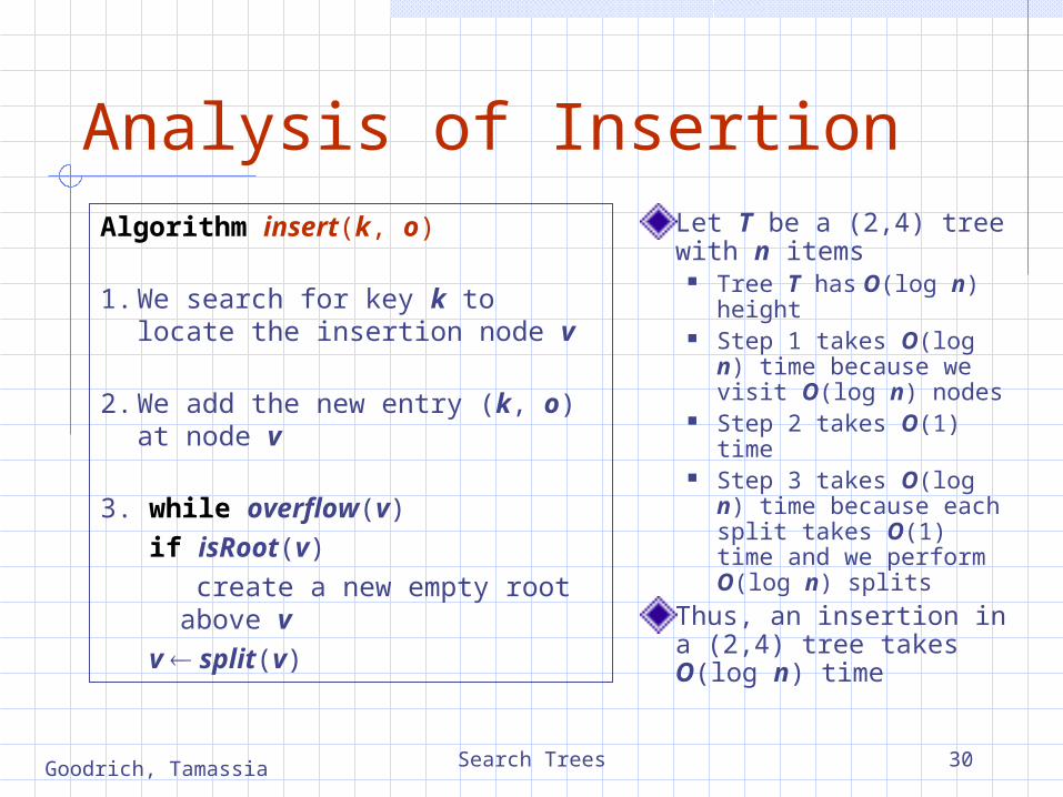
Analysis of InsertionAlgorithm insert(k, o)

1. We search for key k to locate the insertion node v

2. We add the new entry (k, o) at node v

3. while overflow(v)

if isRoot(v)

create a new empty root above v

v split(v)

Let T be a (2,4) tree with n items

Tree T has O(log n) height

Step 1 takes O(log n) time because we visit O(log n) nodes

Step 2 takes O(1) time Step 3 takes O(log n)

time because each split takes O(1) time and we perform O(log n) splits

Thus, an insertion in a (2,4) tree takes O(log n) time


DeletionWe reduce deletion of an entry to the case where the item is at the node with leaf childrenOtherwise, we replace the entry with its inorder successor (or, equivalently, with its inorder predecessor) and delete the latter entryExample: to delete key 24, we replace it with 27 (inorder successor)

27 32 35

10 15 24

2 8 12 18

32 35

10 15 27

2 8 12 18


Underflow and FusionDeleting an entry from a node v may cause an underflow, where node v becomes a 1-node with one child and no keysTo handle an underflow at node v with parent u, we consider two casesCase 1: the adjacent siblings of v are 2-nodes

Fusion operation: we merge v with an adjacent sibling w and move an entry from u to the merged node v'

After a fusion, the underflow may propagate to the parent u

9 14

2 5 7 10

u

v

9

10 14

u

v'w2 5 7


Underflow and TransferTo handle an underflow at node v with parent u, we consider two casesCase 2: an adjacent sibling w of v is a 3-node or a 4-node

Transfer operation:1. we move a child of w to v 2. we move an item from u to v3. we move an item from w to u

After a transfer, no underflow occurs

4 9

6 82

u

vw

4 8

62 9

u

vw


Analysis of Deletion

Let T be a (2,4) tree with n items Tree T has O(log n) height

In a deletion operation We visit O(log n) nodes to locate the node

from which to delete the entry We handle an underflow with a series of

O(log n) fusions, followed by at most one transfer

Each fusion and transfer takes O(1) time

Thus, deleting an item from a (2,4) tree takes O(log n) time


Implementing a DictionaryComparison of efficient dictionary implementations

Search

Insert Delete Notes

Hash Table

1expected

1expected

1expected

no ordered dictionary methods

simple to implement

Skip List

log nhigh prob.

log nhigh prob.

log nhigh prob.

randomized insertion

simple to implement

(2,4) Tree

log nworst-case

log nworst-case

log nworst-case

complex to implement


Red-Black Trees

6

3 8

4

v

z


From (2,4) to Red-Black Trees

A red-black tree is a representation of a (2,4) tree by means of a binary tree whose nodes are colored red or blackIn comparison with its associated (2,4) tree, a red-black tree has

same logarithmic time performance simpler implementation with a single node type

2 6 73 54

4 6

2 7

5

3

3

5OR


Red-Black Trees (§ 9.5)A red-black tree can also be defined as a binary search tree that satisfies the following properties:

Root Property: the root is black External Property: every leaf is black Internal Property: the children of a red node are black Depth Property: all the leaves have the same black depth

9

154

62 12

7

21


Height of a Red-Black TreeTheorem: A red-black tree storing n entries has height O(log n)

Proof: The height of a red-black tree is at most twice the

height of its associated (2,4) tree, which is O(log n)

The search algorithm for a binary search tree is the same as that for a binary search treeBy the above theorem, searching in a red-black tree takes O(log n) time


InsertionTo perform operation insert(k, o), we execute the insertion algorithm for binary search trees and color red the newly inserted node z unless it is the root

We preserve the root, external, and depth properties If the parent v of z is black, we also preserve the internal

property and we are done Else (v is red ) we have a double red (i.e., a violation of the

internal property), which requires a reorganization of the treeExample where the insertion of 4 causes a double red:

6

3 8

6

3 8

4z

v v

z


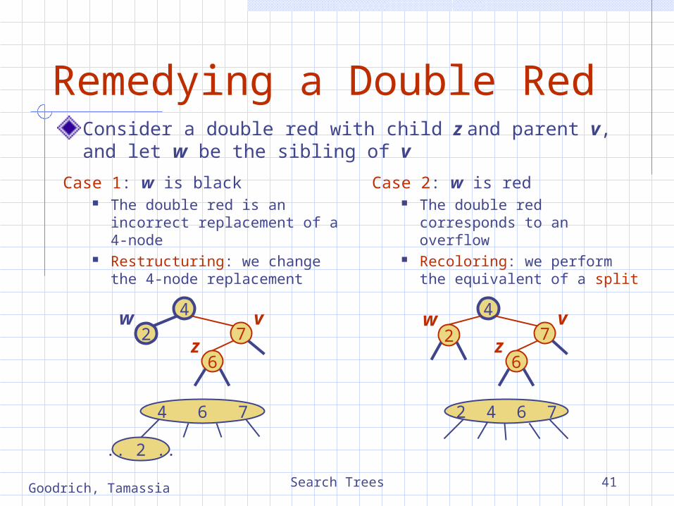
Remedying a Double RedConsider a double red with child z and parent v, and let w be the sibling of v

4

6

7z

vw2

4 6 7

.. 2 ..

Case 1: w is black The double red is an incorrect

replacement of a 4-node Restructuring: we change the

4-node replacement

Case 2: w is red The double red

corresponds to an overflow Recoloring: we perform the

equivalent of a split

4

6

7z

v

2 4 6 7

2w


RestructuringA restructuring remedies a child-parent double red when the parent red node has a black siblingIt is equivalent to restoring the correct replacement of a 4-nodeThe internal property is restored and the other properties are preserved

4

6

7z

vw2

4 6 7

.. 2 ..

4

6

7

z

v

w2

4 6 7

.. 2 ..


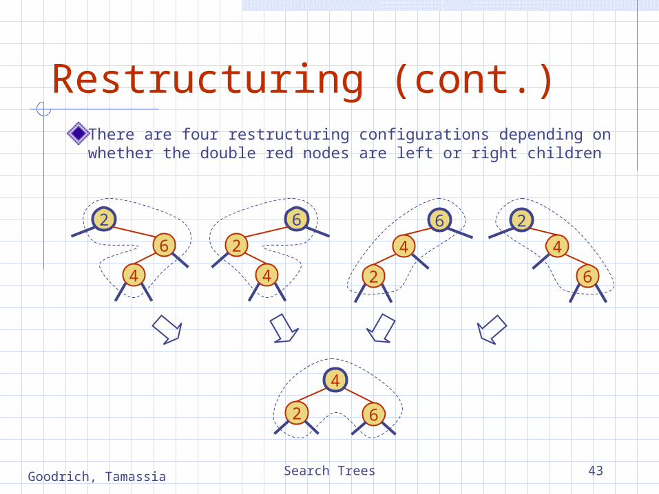
Restructuring (cont.)There are four restructuring configurations depending on whether the double red nodes are left or right children

2

4

6

6

2

4

6

4

2

2

6

4

2 6

4


RecoloringA recoloring remedies a child-parent double red when the parent red node has a red siblingThe parent v and its sibling w become black and the grandparent u becomes red, unless it is the rootIt is equivalent to performing a split on a 5-nodeThe double red violation may propagate to the grandparent u

4

6

7z

v

2 4 6 7

2w

4

6

7z

v

6 7

2w

… 4 …

2


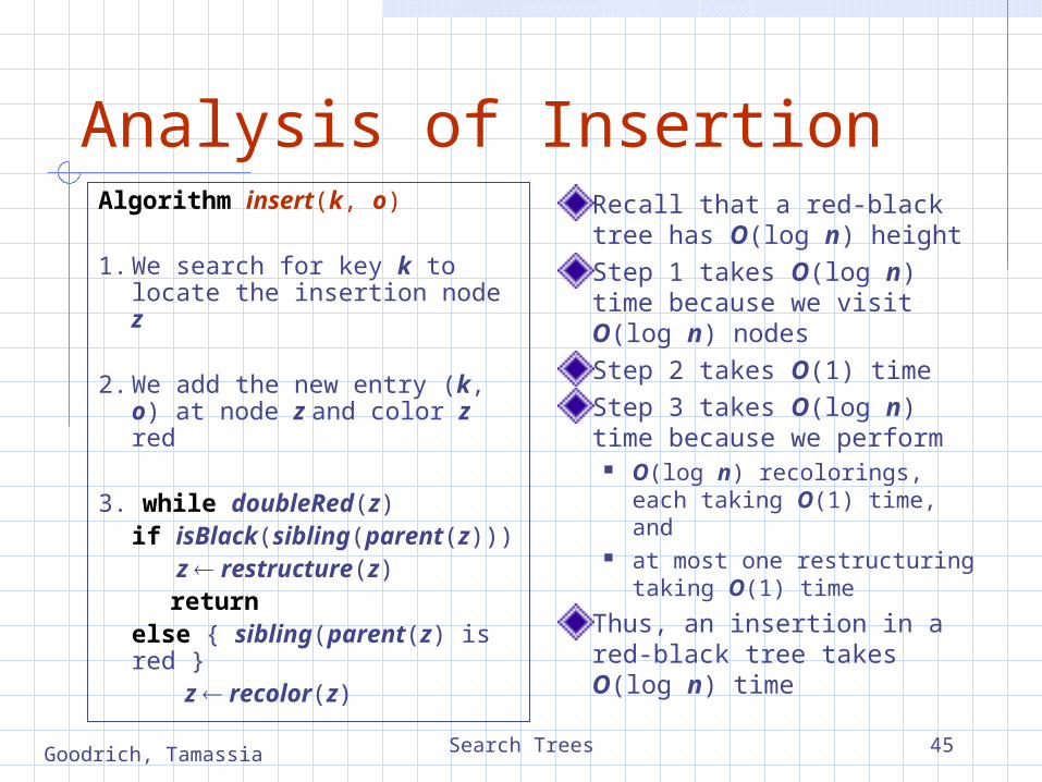
Analysis of InsertionRecall that a red-black tree has O(log n) height

Step 1 takes O(log n) time because we visit O(log n) nodes

Step 2 takes O(1) time

Step 3 takes O(log n) time because we perform

O(log n) recolorings, each taking O(1) time, and

at most one restructuring taking O(1) time

Thus, an insertion in a red-black tree takes O(log n) time

Algorithm insert(k, o)

1. We search for key k to locate the insertion node z

2. We add the new entry (k, o) at node z and color z red

3. while doubleRed(z)if isBlack(sibling(parent(z)))

z restructure(z)return

else { sibling(parent(z) is red } z recolor(z)


DeletionTo perform operation remove(k), we first execute the deletion algorithm for binary search treesLet v be the internal node removed, w the external node removed, and r the sibling of w

If either v of r was red, we color r black and we are done Else (v and r were both black) we color r double black,

which is a violation of the internal property requiring a reorganization of the tree

Example where the deletion of 8 causes a double black:6

3 8

4

v

r w

6

3

4

r


Remedying a Double BlackThe algorithm for remedying a double black node w with sibling y considers three casesCase 1: y is black and has a red child

We perform a restructuring, equivalent to a transfer , and we are done

Case 2: y is black and its children are both black We perform a recoloring, equivalent to a fusion, which may

propagate up the double black violationCase 3: y is red

We perform an adjustment, equivalent to choosing a different representation of a 3-node, after which either Case 1 or Case 2 applies

Deletion in a red-black tree takes O(log n) time


Red-Black Tree ReorganizationInsertion remedy double

red

Red-black tree action (2,4) tree action result

restructuringchange of 4-node representation

double red removed

recoloring splitdouble red removed or propagated upDeletion remedy double

black

Red-black tree action (2,4) tree action result

restructuring transferdouble black removed

recoloring fusiondouble black removed or propagated up

adjustmentchange of 3-node representation

restructuring or recoloring follows


Splay Trees6

3 8

4

v

z


all the keys in the yellow region are 20

all the keys in the blue region are 20

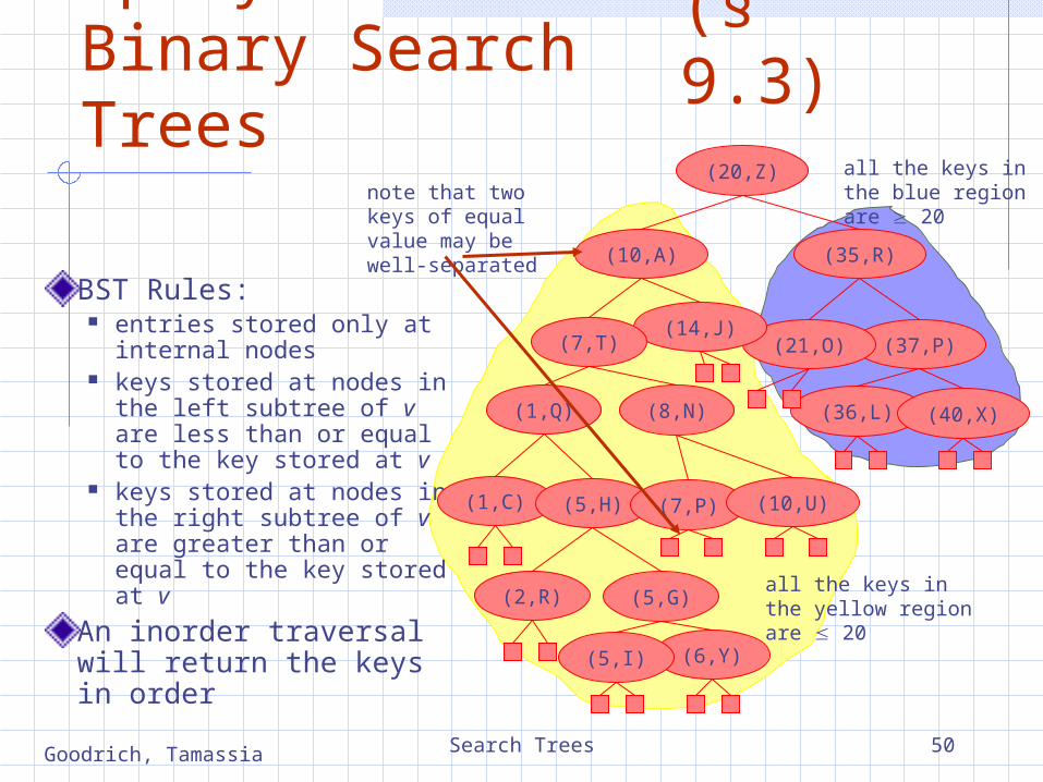
Splay Trees are Binary Search Trees

BST Rules: entries stored only at

internal nodes keys stored at nodes in

the left subtree of v are less than or equal to the key stored at v

keys stored at nodes in the right subtree of v are greater than or equal to the key stored at v

An inorder traversal will return the keys in order

(20,Z)

(37,P)(21,O)(14,J)

(7,T)

(35,R)(10,A)

(1,C)

(1,Q)

(5,G)(2,R)

(5,H)

(6,Y)(5,I)

(8,N)

(7,P)

(36,L)

(10,U)

(40,X)

note that two keys of equal value may be well-separated

(§ 9.3)


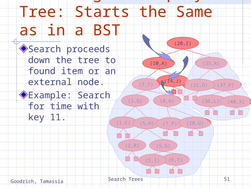
Searching in a Splay Tree: Starts the Same as in a BST

Search proceeds down the tree to found item or an external node.Example: Search for time with key 11.

(20,Z)

(37,P)(21,O)(14,J)

(7,T)

(35,R)(10,A)

(1,C)

(1,Q)

(5,G)(2,R)

(5,H)

(6,Y)(5,I)

(8,N)

(7,P)

(36,L)

(10,U)

(40,X)


Example Searching in a BST, continued

search for key 8, ends at an internal node.

(20,Z)

(37,P)(21,O)(14,J)

(7,T)

(35,R)(10,A)

(1,C)

(1,Q)

(5,G)(2,R)

(5,H)

(6,Y)(5,I)

(8,N)

(7,P)

(36,L)

(10,U)

(40,X)


Splay Trees do Rotations after Every Operation (Even Search)

new operation: splay splaying moves a node to the root using rotations

right rotation makes the left child x of a node y into

y’s parent; y becomes the right child of x

y

x

T1 T2

T3

y

x

T1

T2T3

left rotation makes the right child y of a node x

into x’s parent; x becomes the left child of y

y

x

T1 T2

T3

y

x

T1

T2T3

(structure of tree above y is not modified)

(structure of tree above x is not modified)

a right rotation about y a left rotation about x


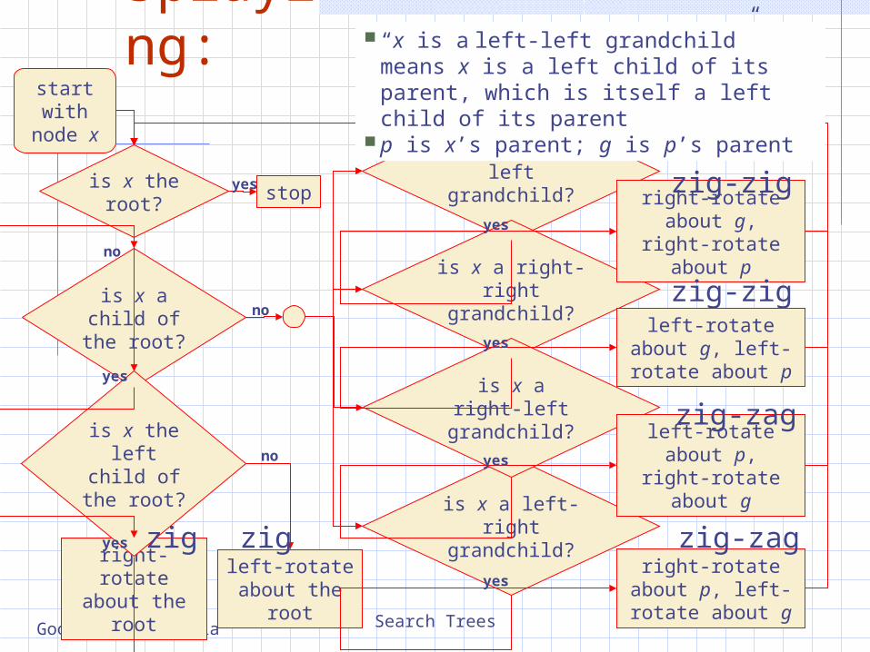
Splaying:

is x the root?

stop

is x a child of the root?

right-rotate about the root

left-rotate about the root

is x the left child of the

root?

is x a left-left grandchild?

is x a left-right grandchild?

is x a right-right grandchild?

is x a right-left grandchild?

right-rotate about g, right-rotate about p

left-rotate about g, left-rotate about p

left-rotate about p, right-rotate about g

right-rotate about p, left-rotate about g

start with node x

“x is a left-left grandchild” means x is a left child of its parent, which is itself a left child of its parent

p is x’s parent; g is p’s parent

no

yes

yes

yes

yes

yes

yes

no

no

yes zig-zig

zig-zag

zig-zag

zig-zig

zigzig


Visualizing the Splaying Cases

zig-zag

y

x

T2 T3

T4

z

T1

y

x

T2 T3 T4

z

T1

y

x

T1 T2

T3

z

T4

zig-zig

y

z

T4T3

T2

x

T1

zig

x

w

T1 T2

T3

y

T4

y

x

T2 T3 T4

w

T1


Splaying Examplelet x = (8,N)

x is the right child of its parent, which is the left child of the grandparent

left-rotate around p, then right-rotate around g

(20,Z)

(37,P)(21,O)(14,J)

(7,T)

(35,R)(10,A)

(1,C)

(1,Q)

(5,G)(2,R)

(5,H)

(6,Y)(5,I)

(8,N)

(7,P)

(36,L)

(10,U)

(40,X)

x

g

p

(10,A)

(20,Z)

(37,P)(21,O)

(35,R)

(36,L) (40,X)(7,T)

(1,C)

(1,Q)

(5,G)(2,R)

(5,H)

(6,Y)(5,I)

(14,J)(8,N)

(7,P)

(10,U)

x

g

p (10,A)

(20,Z)

(37,P)(21,O)

(35,R)

(36,L) (40,X)

(7,T)

(1,C)

(1,Q)

(5,G)(2,R)

(5,H)

(6,Y)(5,I)

(14,J)

(8,N)

(7,P)

(10,U)

x

g

p

1.(before rotating)

2.(after first rotation) 3.

(after second rotation)

x is not yet the root, so we splay again


Splaying Example, Continued

now x is the left child of the root right-rotate around root

(10,A)

(20,Z)

(37,P)(21,O)

(35,R)

(36,L) (40,X)

(7,T)

(1,C)

(1,Q)

(5,G)(2,R)

(5,H)

(6,Y)(5,I)

(14,J)

(8,N)

(7,P)

(10,U)

x

(10,A)

(20,Z)

(37,P)(21,O)

(35,R)

(36,L) (40,X)

(7,T)

(1,C)

(1,Q)

(5,G)(2,R)

(5,H)

(6,Y)(5,I)

(14,J)

(8,N)

(7,P)

(10,U)

x

1.(before applying rotation)

2.(after rotation)

x is the root, so stop


Example Result of Splayingtree might not be more balancede.g. splay (40,X)

before, the depth of the shallowest leaf is 3 and the deepest is 7

after, the depth of shallowest leaf is 1 and deepest is 8

(20,Z)

(37,P)(21,O)(14,J)

(7,T)

(35,R)(10,A)

(1,C)

(1,Q)

(5,G)(2,R)

(5,H)

(6,Y)(5,I)

(8,N)

(7,P)

(36,L)

(10,U)

(40,X)

(20,Z)

(37,P)

(21,O)

(14,J)(7,T)

(35,R)

(10,A)

(1,C)

(1,Q)

(5,G)(2,R)

(5,H)

(6,Y)(5,I)

(8,N)

(7,P) (36,L)(10,U)

(40,X)

(20,Z)

(37,P)

(21,O)

(14,J)(7,T)

(35,R)

(10,A)

(1,C)

(1,Q)

(5,G)(2,R)

(5,H)

(6,Y)(5,I)

(8,N)

(7,P)

(36,L)

(10,U)

(40,X)

before

after first splay after second splay


Splay Tree Definition

a splay tree is a binary search tree where a node is splayed after it is accessed (for a search or update) deepest internal node accessed is

splayed splaying costs O(h), where h is height

of the tree – which is still O(n) worst-case O(h) rotations, each of which is O(1)


Splay Trees & Ordered Dictionaries

which nodes are splayed after each operation?

use the parent of the internal node that was actually removed from the tree (the parent of the node that the removed item was swapped with)remove(k)

use the new node containing the entry insertedinsert(k,v)

if key found, use that node

if key not found, use parent of ending external nodefind(k)

splay nodemethod


Amortized Analysis of Splay Trees

Running time of each operation is proportional to time for splaying.Define rank(v) as the logarithm (base 2) of the number of nodes in subtree rooted at v.Costs: zig = $1, zig-zig = $2, zig-zag = $2.Thus, cost for playing a node at depth d = $d.Imagine that we store rank(v) cyber-dollars at each node v of the splay tree (just for the sake of analysis).


Cost per zig

Doing a zig at x costs at most rank’(x) - rank(x): cost = rank’(x) + rank’(y) - rank(y) - rank(x)

< rank’(x) - rank(x).

zig

x

w

T1 T2

T3

y

T4

y

x

T2 T3 T4

w

T1


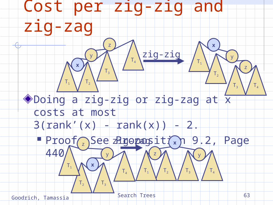
Cost per zig-zig and zig-zag

Doing a zig-zig or zig-zag at x costs at most 3(rank’(x) - rank(x)) - 2. Proof: See Proposition 9.2, Page 440.

y

x

T1 T2

T3

z

T4

zig-zig y

z

T4T3

T2

x

T1

zig-zagy

x

T2 T3

T4

z

T1

y

x

T2 T3 T4

z

T1


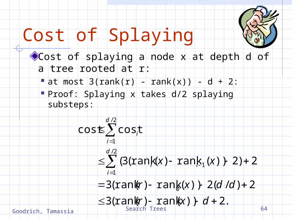
Cost of SplayingCost of splaying a node x at depth d of a tree rooted at r: at most 3(rank(r) - rank(x)) - d + 2: Proof: Splaying x takes d/2 splaying substeps:

.2))(rank)(rank(3

2)/(2))(rank)(rank(3

2)2))(rank)(rank(3(

cost cost

0

1

2/

1

2/

1

dxr

ddxr

xx i

d

ii

i

d

i


Performance of Splay Trees

Recall: rank of a node is logarithm of its size.Thus, amortized cost of any splay operation is O(log n).In fact, the analysis goes through for any reasonable definition of rank(x).This implies that splay trees can actually adapt to perform searches on frequently-requested items much faster than O(log n) in some cases. (See Proposition 9.4 and 9.5.)

goodrich, tamassia search trees1 binary search trees 6 9 2 4 1 8

Documents

tamassia search trees6

binary search insert

w w slide

tamassia search trees2

node w

node v

binary tree

isexternal v return