government budget and chapter fiscal...
TRANSCRIPT

11CHAPTERGovernment Budget and
Fiscal Policy
The National Budget
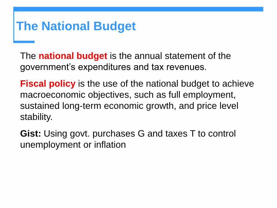
The national budget is the annual statement of the
government’s expenditures and tax revenues.
Fiscal policy is the use of the national budget to achieve
macroeconomic objectives, such as full employment,
sustained long-term economic growth, and price level
stability.
Gist: Using govt. purchases G and taxes T to control
unemployment or inflation

The National Budget
The government’s budget balance equals tax revenue
minus expenditure.
If tax revenues exceed expenditures, the government has
a budget surplus [T>G].
If expenditures exceed tax revenues, the government has
a budget deficit [G>T].
If tax revenues equal expenditures, the government has a
balanced budget [T=G].

The Federal Budget - USA
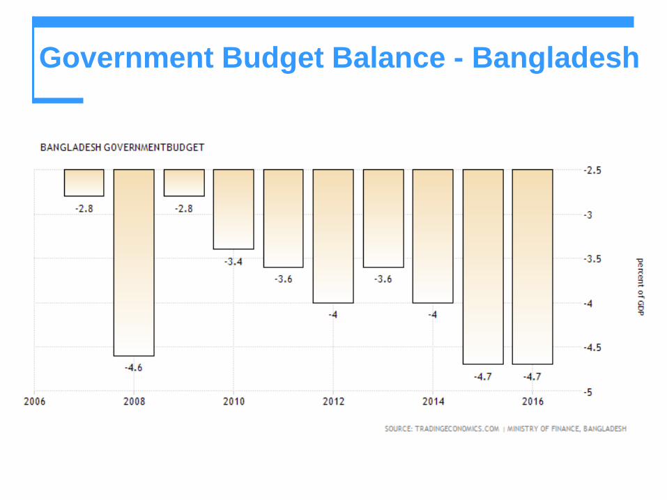
Government Budget Balance - Bangladesh

This Figure shows receipts as a percentage of GDP.
Receipts
Federal Receipts - USA

Federal Receipts - USA
Social Security tax
The tax levied on both employers and employees used to
fund the Social Security program. The Social Security tax
pays for the retirement and disability benefits received by
millions of Americans each year.
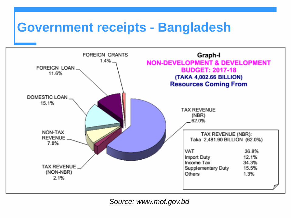
Government receipts - Bangladesh
Source: www.mof.gov.bd

The Federal Outlays - USA
This Figure shows outlays as a percentage of GDP.
Outlays

Government Outlays - Bangladesh
Source: www.mof.gov.bd

The National Budget
Cyclical Deficits and Structural Deficits
Suppose the budget is currently balanced, and then Real GDP in the
economy drops.
As Real GDP drops, the tax base of the economy falls, and, if tax rates
are held constant, tax revenues will fall.
Another result of the decline in Real GDP is that transfer payments (e.g.,
unemployment compensation) will rise.
Thus, government expenditures will rise as tax revenues fall.
As a result, a balanced budget turns into a budget deficit—a result of the
downturn in economic activity, not from current spending and taxing
decisions by the government.

The National Budget
Cyclical Deficits and Structural Deficits
Economists use the term cyclical deficit to describe
budget deficit that is a result of a downturn in economic
activity.
On the other hand deficit that would exist if the economy
were operating at full employment—is called the structural
deficit.

The National Budget
This Figure illustrates a
cyclical deficit and a
cyclical surplus.
In part (a), potential GDP
is $14 trillion.
If real GDP is $13 trillion,
the budget is in deficit and
it is a cyclical deficit.
If real GDP is $15 trillion,
the budget is in surplus
and it is a cyclical surplus.

The National Budget
In part (b), if real GDP and potential GDP are $13 trillion, the budget is a deficit and the deficit is a structural deficit.
If real GDP and potential GDP are $14 trillion, the budget is balanced.
If real GDP and potential GDP are $15 trillion, the budget is a surplus and the surplus is a structural surplus.
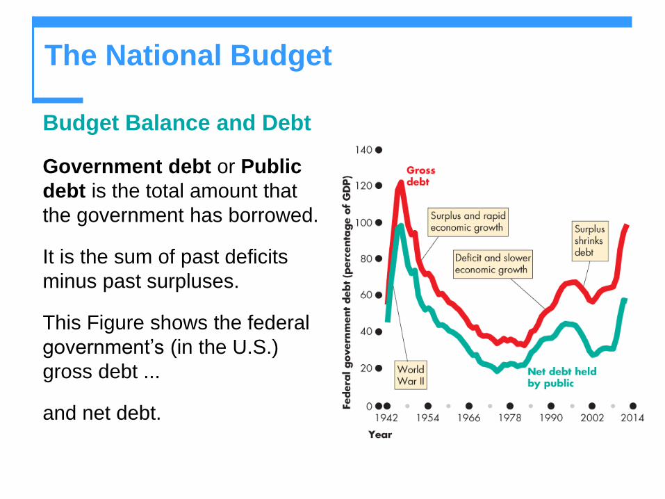
Budget Balance and Debt
Government debt or Public
debt is the total amount that
the government has borrowed.
It is the sum of past deficits
minus past surpluses.
This Figure shows the federal
government’s (in the U.S.)
gross debt ...
and net debt.
The National Budget

Government enters the loanable funds market when it has
a budget surplus or deficit.
A government budget surplus increases the supply of
funds.
A government budget deficit increases the demand for
funds.
Budget Deficit and the Crowding-Out Effect
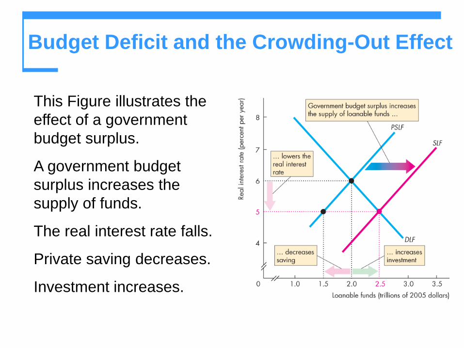
This Figure illustrates the
effect of a government
budget surplus.
A government budget
surplus increases the
supply of funds.
The real interest rate falls.
Private saving decreases.
Investment increases.
Budget Deficit and the Crowding-Out Effect

This Figure illustrates the
effect of a government
budget deficit.
A government budget
deficit increases the
demand for funds.
The real interest rate rises.
Private saving increases.
Investment decreases—is
crowded out.
Budget Deficit and the Crowding-Out Effect

This Figure illustrates the
Ricardo-Barro effect.
A budget deficit increases the
demand for funds.
Rational taxpayers increase
saving, which increases the
supply of funds.
Increased private saving
finances the deficit.
Crowding-out is avoided.
Budget Deficit and the Crowding-Out Effect

Fiscal Policy Multipliers
Before we discuss fiscal policy and it’s effect on real
GDP and price level, we need to make the following
assumptions:
Economy is not self regulating when it is in a recessionary
gap (similar to Keynesian assumption).
Price is not constant in the short run, i.e., SRAS is upward
sloping (similar to Classical view).
So, we are somewhere in between the Classical and the
Keynesian model.
Fiscal Policy Multipliers
Automatic fiscal policy is a change in fiscal policy triggered
automatically by the state of the economy. To illustrate, suppose Real
GDP in the economy turns down, causing more people to become
unemployed and, as a result, automatically receive unemployment
benefits. These added unemployment benefits automatically boost
government spending.
Discretionary fiscal policy is a policy action that is initiated by an act
of the Government, taken deliberately.
To enable us to focus on the principles of fiscal policy multipliers, we
first study discretionary fiscal policy in a model economy that has only
“lump-sum” taxes.
Lump-sum taxes are taxes that do not vary with real GDP; actual
examples would be a ‘head tax’ or property taxes.

Fiscal Policy Multipliers
The Government Purchases Multiplier
The government purchases multiplier is the
magnification effect of a change in government purchases
of goods and services on equilibrium aggregate
expenditure and real GDP.
A multiplier exists because government purchases are a
component of aggregate expenditure; an increase in
government purchases increases aggregate income,
which induces additional consumption expenditure.

Fiscal Policy Multipliers
This Figure illustrates
the government
purchases multiplier in
the aggregate
expenditure diagram.
The government
purchases multiplier is
1/(1 – MPC) where MPC is
the marginal propensity to
consume (absent induced
taxes and imports).

Fiscal Policy Multipliers
The Lump-Sum Tax Multiplier
The lump-sum tax multiplier is the magnification effect a
change in lump-sum taxes has on equilibrium aggregate
expenditure and real GDP.
An increase in lump-sum taxes decreases disposable
income, which decreases consumption expenditure and
decreases aggregate expenditure and real GDP.

Fiscal Policy Multipliers
The amount by which a tax increase lowers consumption
expenditure is determined by the MPC.
A $1 tax increase lowers consumption expenditure by $1
MPC, and this amount gets multiplied by the standard
autonomous expenditures multiplier.
The lump-sum tax multiplier is therefore -[MPC/(1 –
MPC)].
It is negative because an increase in lump-sum taxes
decreases equilibrium expenditure.

Fiscal Policy Multipliers
This Figure illustrates
the effect of an increase
in lump-sum taxes.
The lump-sum transfer
payments multiplier and
the lump-sum tax multiplier
are the same except for
their signs—the transfer
payments multiplier is
positive.
Fiscal Policy Multipliers
Induced Taxes and Entitlement Spending
Taxes that vary with real GDP are called induced taxes.
Most transfer payments are part of entitlement spending,
and they vary with real GDP – they are induced, too.
During a recession, induced taxes fall and entitlement
spending rises; and during an expansion, induced taxes
rise and entitlement spending falls. For this reason, they
are called automatic stabilizers.
Both effects also diminish the size of the government
purchases and lump-sum tax multipliers.
Fiscal Policy Multipliers
International Trade and Fiscal Policy Multipliers
Imports also decrease the fiscal policy multipliers.
The larger the marginal propensity to import, the smaller is
the magnitude of the government purchases and lump-
sum tax multipliers. The reason? If a bigger fraction of any
change in aggregate income is spent on imports, a smaller
fraction is spent on domestically-produced output so
generates less GDP and income.
Remember the multiplier formula with imports?
Multiplier =1
1− 𝑏 1−𝑡 −𝑚

Fiscal Policy Multipliers
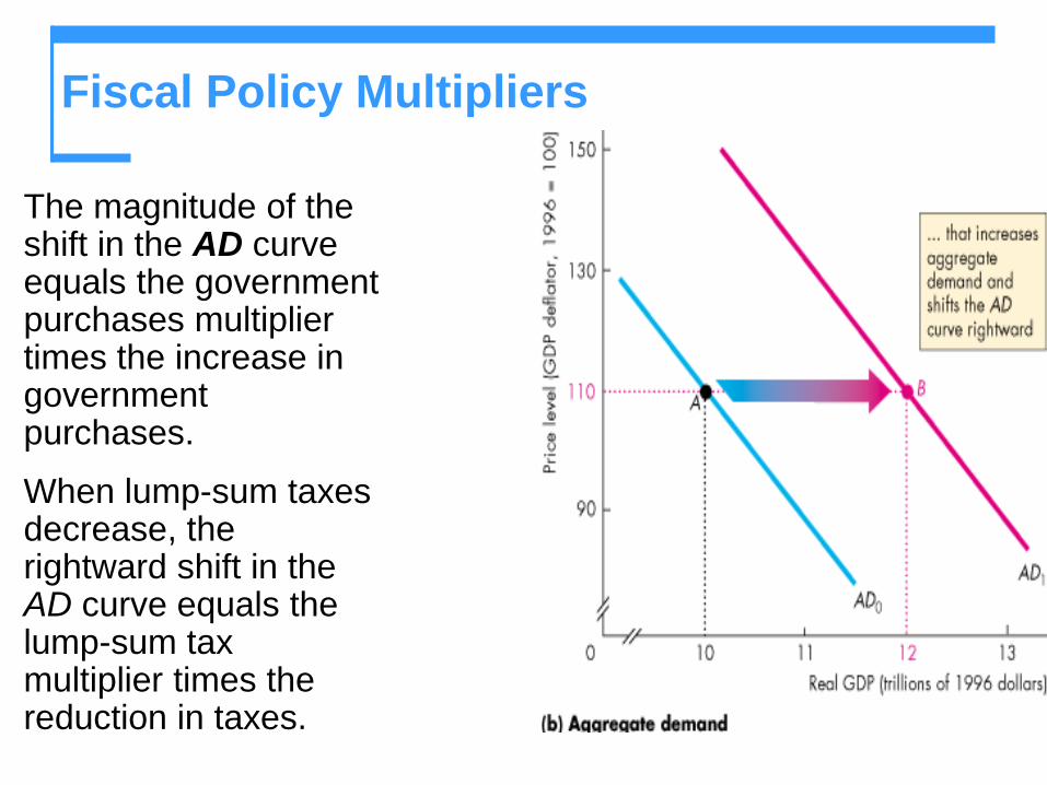
Fiscal Policy and
Aggregate Demand
This Figure illustrates
the effects of fiscal
policy on aggregate
demand.
An increase in
government
purchases shifts the
AE curve upward
and shifts the AD
curve rightward.
Fiscal Policy Multipliers
The magnitude of the shift in the AD curve equals the government purchases multiplier times the increase in government purchases.
When lump-sum taxes decrease, the rightward shift in the AD curve equals the lump-sum tax multiplier times the reduction in taxes.
Fiscal Policy
Expansionary fiscal policy, an increase in government
expenditures (𝐺) or a decrease in taxes (𝑇), shifts the AD
curve to the right. The target of an expansionary fiscal
policy is to increase production and reduce unemployment.
The underlying assumption is that the economy is in a
recessionary gap.
Contractionary fiscal policy, a decrease in government
expenditures (𝐺) or an increase in taxes (𝑇), shifts the AD
curve to the left. The target of an contractionary fiscal policy
is to decrease production and reduce inflation. The
underlying assumption is that the economy is in an
inflationary gap.

Fiscal Policy
Graphical Illustration of
Fiscal Stimulus
This Figure shows how fiscal policy
is supposed to work to close a
recessionary gap.
An increase in government
expenditure or a tax cut increases
aggregate expenditure.
The multiplier process increases
aggregate demand.
If no supply side effect is present,
then ∆𝑇 would need be larger than
∆𝐺 to get GDP to potential GDP.

Fiscal Policy
Fiscal Expansion at
Potential GDP
This Figure
illustrates the
effects of an
expansionary fiscal
policy starting from
a position of full
employment.

Fiscal Policy
So, if the economy was
at potential GDP to begin
with, then in the long run,
fiscal policy multipliers
are zero because real
GDP equals potential
GDP and a change in
aggregate demand
changes the money
wage rate, the SAS
curve, and the price
level.
Limitations of Fiscal Policy
Because the short-run fiscal policy multipliers are not
zero, fiscal policy can be used to help stabilize the
economy, and frequently is in countries with
parliamentary systems of government [or other systems
that allow the executive to control the budget].
But in practice, fiscal policy is always hard to use, and in
the US usually not feasible, because:
The legislative process is too slow to permit fiscal policy actions
to be implemented when they are needed.
Potential GDP is very hard to estimate, so the wrong fiscal
stimulus or restraint may be enacted.

Limitations of Fiscal Policy
Fiscal Policy May Destabilize the
Economy
In this scenario, the 𝑆𝑅𝐴𝑆 curve is
shifting rightward (healing the
economy of its recessionary gap),
but this information is unknown to
policy makers. Policy makers
implement expansionary fiscal
policy, and the 𝐴𝐷 curve ends up
intersecting 𝑆𝑅𝐴𝑆2 at point 2
instead of intersecting 𝑆𝑅𝐴𝑆1 at
point 1′. Policy makers thereby
move the economy into an
inflationary gap, thus destabilizing
the economy.

Supply-Side Effects of Fiscal Policy
Fiscal Policy and Aggregate Supply
Production depends on the quantity of labor, which in turn
is influenced by the income tax.
Figure on the next slide illustrates the effect of the income
tax in the labor market.

Supply-Side Effects of Fiscal Policy
The income tax
decreases the
aggregate supply of
labor because it
decreases the after-
tax wage rate.
Because the income tax
decreases the aggregate
supply of labor, it raises
the equilibrium wage rate,
decreases employment,
and decreases aggregate
supply.

Supply-Side Effects of Fiscal Policy
This supply-side effect of the income tax means that a cut in the income tax rate may increase aggregate supply.

Supply Side Effects of Fiscal Policy
This Figure illustrates
two views about the
effects of a tax cut on
real GDP and the
price level (assuming
the economy is in a
recessionary gap).
A tax cut increases
aggregate demand
and the AD curve
shifts rightward.

Supply-Side Effects of Fiscal Policy
Most economists
believe that a tax
cut has a small
effect on aggregate
supply [SAS0 to
SAS1].
So GDP increases
and the price level
rises.

Supply-Side Effects of Fiscal Policy
Supply-side
economists think that
a tax cut may
increase aggregate
supply by a large
amount [SAS0 to
SAS2] so that GDP
can increase and the
price level does not
change much (or
maybe even fall).

Tax Rates and Tax Revenues
Laffer Curve
The curve, named after
Arthur Laffer, that shows the
relationship between tax
rates and tax revenues.
According to the Laffer
curve, as tax rates rise from
zero, tax revenues rise,
reach a maximum at some
point, and then fall with
further increases in tax rates.

Tax Rates and Tax Revenues
Laffer Curve
Tax revenues = Tax base × Average Tax rate
As tax rate increases:
Direct effect: Upward pressure on tax revenues
Indirect effect: Downward pressure on tax base →Downward pressure on tax revenues
Tax base is a direct function of Real GDP.
An increase in tax rate puts downward pressure on tax base
because: increased tax rate → both demand and supply curve
(according to supply-side economists) shift leftward → Real GDP
falls → Tax base falls.

Tax Rates and Tax Revenues
Laffer Curve
Between point A and
point B, the direct effect
dominates, so, tax
revenues increase.
Between point B and
point C, the indirect
effect dominates.
Rationale: The greater
the proportion of one’s
income is taken away
in taxes, the lesser the
incentive for working.
At point B, tax revenues
are maximized.

Tax rates in Bangladesh
According to a National Board of Revenue (NBR),
Bangladesh circular, in 2017-18:
Tax free Income
For men less than 65 years of age: Tk. 20,833/month
For women and people over 65 years of age: Tk. 25,000/month
For people with disability: Tk. 31,250/month

Tax rates in Bangladesh
Tax rates
Total Income (Yearly) Tax rate
First 2,50,000 Tk. 0%
Next 4,00,000 Tk. 10%
Next 5,00,000 Tk. 15%
Next 6,00,000 Tk. 20%
Next 30,00,000 Tk. 25%
Any remaining income 30%