Department of Economics

Econometrics Working Paper EWP0501

ISSN 1485-6441

GOVERNMENT SIZE AND ECONOMIC GROWTH: TIME-SERIES EVIDENCE FOR THE UNITED KINGDOM, 1830-1993

Wing Yuk

Department of Economics, University of Victoria Victoria, B.C., Canada V8W 2Y2

January, 2005

Author Contact: Wing Yuk, P.O. Box 37063 RPO, Vancouver, BC, Canada V5P 4W7.

Tel: +1-604-782-8081; email: wingyuk2004@yahoo.com

Abstract

This study considers the long-run relationship between government expenditure and economic growth for

the United Kingdom over the period 1830 to 1993. The causality analysis allows for the effects of exports,

and for the presence of complex structural breaks in the data. The results support the export-led growth

hypothesis. Although support for Wagner’s Law is sensitive to the choice of sample period, there is

evidence that GDP growth Granger-causes the share of government spending in GDP indirectly through

exports’ share of GDP during the period 1870-1930.

Keywords: Wagner’s Law; Granger causality; size of government; structural breaks JEL Classifications: C32, H50, O4

I. INTRODUCTION

Economic growth is one of the most fascinating topics in macroeconomics. Among the factors

that determine the growth of an economy, government spending is of particular interest in this

paper. Empirical studies of the impact of government expenditure on long-run economic growth

include, among others, Feder (1983), Landau (1983), Ram (1986), Grier and Tullock (1989),

Romer (1990), Barro (1990, 1991), Levine and Renelt (1992), Devarajan et al. (1996), and Sala-i-

Martin (1997). Most of these studies used cross-section data to link measures of government

spending with economic growth rates. The disadvantage of such studies is that “cross-sectional

analysis can identify correlation but not causation between variables” (Hsieh and Lai, 1994)

because it provides only “pooled estimates of the effects of government size on economic

growth” (Ghali, 1999), and it fails to disentangle the effects for each country.

Traditional OLS regression analysis is not sufficient to determine the flow(s) of causality. When

economic growth is regressed on government spending, researchers tend to interpret this as a

confirmation of causality from the latter to the former. However, a significant coefficient can be

equally compatible with the Keynesian view (causality from government expenditure to growth),

Wagner’s Law (from growth to spending), and/or a bi-directional causality between the two

variables. The proper way to deal with this, as suggested by Ghali (1999), is to use Granger

causality testing. His results indicated that government size did matter in determining the

economic growth for all OECD countries in a positive way, thereby supporting the Keynesian

View. Hsieh and Lai (1994), on the other hand, concluded that there was no evidence of Granger

causality from government expenditure to per capita output growth for the G-7 countries.

Building on Ghali’s (1999) work, this paper models the relationship between GDP, the share of

government spending in GDP, and the share of exports in GDP within a time-series framework.

The remainder of this paper is organized as follows. In section II, we consider some of the past

literature on Wagner’s Law. Section III introduces our methodology and section IV discusses

data issues (including non-stationarity, cointegration and structural breaks). The results of our

causality analysis appear in section V, and the final section VI provides some conclusions and

suggestions for further research.

II. WAGNER’S LAW

Writing in 1890, Adolph Wagner formulated the ‘Law of the Increasing Extension of State

Activity’, commonly referred to as Wagner’s Law. It is one of the theories that emphasize

economic growth as the fundamental determinant of public sector growth, and has since been the

focus of many empirical studies. Wahab (2004) intended to disentangle the effects of accelerating

and decelerating economic growth in government expenditure for OECD, EU and G7 countries

for the period 1950-2000. He found evidence of Wagner’s law for EU countries only. However,

his findings suggested that, for all countries in general, government expenditure increased less

than proportionately with accelerating growth and decreased more than proportionately with

decelerating economic growth. Quite contrary, the study by Kolluri et al. (2000), which focused

on the relationship between economic growth and certain components of public expenditures1 of

the G7 countries2 for the period 1960-1993, provided inconsistent results. Wagner’s Law was

confirmed for all 7 countries3, i.e., there were signs of long-run equilibrium relationships between

different categories of government spending and economic growth. For the UK in particular,

Wagner’s Law was confirmed for all three categories of public expenditure given the positive

signs on the coefficients.

A disadvantage of the studies by Wahab (2002) and Kolluri et al. (2000), however, is that it did

not study the Keynesian View. In an earlier study by Ghali (1999), he studied the causal

relationships between government expenditures and economic growth for ten OECD countries4

using a quarterly data set covered the period 1970:1 to 1994:3. His results supported the

Keynesian view, but there was no evidence of Wagner’s Law. In another study by Oxley (1994),

which focused on the UK exclusively for the period 1870 to 1913, his results suggested a uni-

directional causality from national income (GDP) to public expenditure, thereby supporting

Wagner’s Law.

1 The dependent variables that they used were: total government expenditure (GT), total government consumption (GC) and total government transfer expenditure (TE). The independent variable was nominal GDP. 2 G-7countries include Canada, France, Italy, Japan, UK, USA and Germany. 3 There were two exceptions; total government expenditure in France and total government transfer in Canada were not cointegrated with national income.

III. MODEL AND METHODOLOGY

Theoretical ties between international trade and growth have been formalized by Rivera-Batiz and

Romer (1991), Grosman and Helpman (1990), and Romer (1990). It is obvious that the growth of

an economy affects international trade in some way, however, the question of whether exports

lead to growth of an economy or not remains an open question. Hence, the inclusion of such

variable in the analysis gives us more valuable information of the interactions between

international trade and government size. Given the purpose of this study, one limitation of the

ordinary least squares (OLS) approach is that it ignores the fact that many economic systems

exhibit feedback. Take our proposed trivariate model as an example, there appears to be inter-

relationships between the series such that it is difficult to state which one should be the dependent

variable. For example, GDP depends on government expenditure and exports; on the other hand,

however, government expenditure depends on the economic performance of an economy (in

terms of exports and GDP). Therefore, a trivariate VAR model enables us to treat all series

systematically without making reference to the issue of dependence versus independence.

Our VAR model, which includes GDP, share of government spending, and the share of exports to

GDP, is as follows:

yt = ψ0 + ψ1 t + Σ Γi yt-i + εt (1)

where εt ∼ iid (0, Ω), and

LGDPt A10 A11 γ11i γ12i γ13i yt = LSGOVEXPt , ψ0 = A20 , ψ1 = A21 , Γi = γ21i γ22i γ23i , LSEXPORTSt A30 A31 γ31i γ32i γ33i ε1t σ1

2 σ12 σ13

εt = ε2t , and Ω = σ12 σ22

σ23 ε3t σ13 σ23 σ3

2

where “LGDPt” denotes “log of GDP”, “LSGOVEXPt” denotes “the share of government

spending to GDP (in logs)” and “LSEXPORTSt” denotes “the share of exports to GDP (in logs)”.

The data are illustrated in Figures 1 to 3.

4 OECD countries include US, Japan, UK, Australia, Canada, France, Italy, Spain, Switzerland, and Norway.

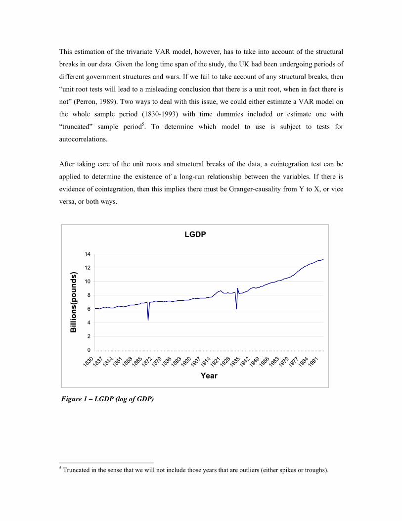
This estimation of the trivariate VAR model, however, has to take into account of the structural

breaks in our data. Given the long time span of the study, the UK had been undergoing periods of

different government structures and wars. If we fail to take account of any structural breaks, then

“unit root tests will lead to a misleading conclusion that there is a unit root, when in fact there is

not” (Perron, 1989). Two ways to deal with this issue, we could either estimate a VAR model on

the whole sample period (1830-1993) with time dummies included or estimate one with

“truncated” sample period5. To determine which model to use is subject to tests for

autocorrelations.

After taking care of the unit roots and structural breaks of the data, a cointegration test can be

applied to determine the existence of a long-run relationship between the variables. If there is

evidence of cointegration, then this implies there must be Granger-causality from Y to X, or vice

versa, or both ways.

LGDP

0

2

4

6

8

10

12

14

1830

1837

1844

1851

1858

1865

1872

1879

1886

1893

1900

1907

1914

1921

1928

1935

1942

1949

1956

1963

1970

1977

1984

1991

Year

Bill

ions

(pou

nds)

Figure 1 – LGDP (log of GDP)

5 Truncated in the sense that we will not include those years that are outliers (either spikes or troughs).

LSGOVEXP

-3.5

-3

-2.5

-2

-1.5

-1

-0.5

0

1830

1837

1844

1851

1858

1865

1874

1881

1888

1895

1902

1909

1916

1923

1930

1940

1947

1954

1961

1968

1975

1982

1989

Year

Bill

ions

(pou

nds)

Figure 2 - LSGOVEXP (log of the share of government expenditure in GDP) in billion pounds

LSEXPORTS

-4

-3.5

-3

-2.5

-2

-1.5

-1

-0.5

0

0.5

1

1.5

1830

1837

1844

1851

1858

1865

1872

1879

1886

1893

1900

1907

1914

1921

1928

1935

1942

1949

1956

1963

1970

1977

1984

1991

Year

Bill

ions

(pou

nds)

Figure 3 - LSEXPORTS (log of the share of exports to GDP) in billion pounds

IV. DATA NON-STATIONARITY AND STRUCTURAL BREAKS

The raw data used in this study are obtained from Mitchell (1998), who provides a good source

for historic long time span data. The period 1830 to 1993 is chosen because as Ram (1992) and

Henrekson (1993) point out, Wagner’s postulate is essentially a statement about the long-run

relationship between economic development and the relative size of the public sector. Hence, any

empirical analysis should base on samples from a relatively longer time frame.

As noted by Granger and Newbold (1974), estimation of non-stationary data with a stochastic

trend will cause spurious regression problems. First, the least squares estimators of the intercept

and slope coefficients are not consistent6. Second, the conventional test statistics, such as the t-

ratio, F-statistic, etc., do not have distributions like t- and F-distributions that we expect to hold

when the null hypothesis is true, not even asymptotically. Consequently, the critical values

normally used are inappropriate. Third, there will be “an apparently high degree of goodness of

fit, as measured by the coefficient of multiple correlation R2 or the ‘corrected’ coefficient R2, but

the Durbin-Watson d statistic will converge to zero as sample size grows7”(Granger and

Newbold, 1974). Fourth, there will be spurious rejections by cointegration tests. In the presence

of neglected structural breaks, Dickey-Fuller tests generate a spurious appearance of trend-

stationarity when in fact the true generating process is difference-stationary - that is, integrated of

order one (Leybourne and Newbold, 2003). Hence, before we could proceed with the Granger

causality test, it is necessary to apply unit root tests on each series of data.

Unit Root Tests

If a time series is differenced d times to be stationary, then the original series is integrated of

order d, denoted by I(d). In order to establish the order of integration, we employ the Augmented

Dickey Fuller (ADF) test by considering the following regressions:

I(1) vs. I(0): yt = δ yt-1 + [ α0 + α1 t + Σ βj ∆ yt-j ] + εt (2)

I(2) vs. I(1) : ∆yt = δ ∆yt-1 + [ α0 + α1 t + Σ βj ∆2 yt-j ] + εt (3)

6 A consistent estimator is one such that it approaches the true parameter value as the sample size gets larger. 7 As the Durbin-Watson statistic (d) approaches zero, it is clear that there is evidence of positive serial correlation.

where εt denotes the errors that are assumed to be correlated across time, t is the linear

deterministic trend, α0 is the drift and ∆ is the difference operator. One drawback of the test,

however, is its assumption of no shift in either level or slope of the series. In reality, we know that

this rarely happens, especially when we deal with this really long time span from 1830 to 1993.

Filling in the Gaps

Given all series display spikes at certain points in time (refer to Figure 1, 2 and 3), we have to

take that into account to avoid any biased results. Fill-up the gaps, delete missing observations,

and linearly interpolate across the gaps are three common options. The last option, however,

ranks the last in terms of size-distortion and power8 (Ryan and Giles, 1998). With regard to the

second option, Vogelsang (1994) showed that the model led to misleading inferences. Hence, the

first option seems to be a better method.

FLGDP

0

2

4

6

8

10

12

14

1830

1837

1844

1851

1858

1865

1874

1881

1888

1895

1902

1909

1916

1923

1930

1940

1947

1954

1961

1968

1975

1982

1989

Year

Bill

ions

(pou

nds)

Figure 4 - FLGDP (Filled log of GDP)

8 At certain points in time, the values were below the significance level (10%).

FLSGOVEXP

-3.5

-3

-2.5

-2

-1.5

-1

-0.5

0

1830

1836

1842

1848

1854

1860

1866

1874

1880

1886

1892

1898

1904

1910

1916

1922

1928

1937

1943

1949

1955

1961

1967

1973

1979

1985

1991

Year

Bill

ions

(pou

nds)

Figure 5 - FLSGOVEXP (Filled log of share of government expenditure to GDP)

FLSEXPORTS

0

2

4

6

8

10

12

14

1830

1837

1844

1851

1858

1865

1874

1881

1888

1895

1902

1909

1916

1923

1930

1940

1947

1954

1961

1968

1975

1982

1989

Year

Bill

ions

(pou

nds)

Figure 6 - FLSEXPORTS (Filled of log of the share of exports to GDP)

To deal with the structural breaks, Perron (1989) proposed a modified DF test9 with three types of

deterministic trend functions, namely Type “A” (the Crash model), Type “B” (the Changing

9 With Perron’s approach, there are two underlying assumptions: first, any shift in level or trend is exogenous; and second, there can only be a one-time change in level and/or trend.

Growth model) and Type “C” (combination of Type “B” and Type “A”). The resulting t-ratios are

to be compared with the critical values10 calculated by Perron.

Different Time Periods

Another technique we use is to test for unit roots in the original data by ignoring the spikes. In

particular, we will separate the whole sample into different time periods. The way we specify

each period is based on the location of the spikes. For the “filled” series of FLGDP, the three sub-

sample periods are 1830-1867, 1869-1930, and 1932-1993. For the “filled” series of

FLSGOVEXP, the three sub-sample periods are 1830-1867, 1869-1930, and 1933-1993. And for

the last series FLSEXPORTS, there are four sub-sample periods: 1830-1867, 1868-1930, 1933-

1993, and 1948-1993.

Bootstrapping Unit Root Tests

For the LGDP series, the unit root test results of both “filled-up” and separate period methods

confirm that the series is non-stationary. The other two series, LSGOVEXP and LSEXPORTS,

however, results are mixed (refer to Table 1). Given these mixed results, a re-sampling bootstrap

(Maddala and Kim, 1998) is employed that takes account of the finite sample characteristics of

our data11. Given our small sample size, bootstrapping enables us to obtain small sample critical

values from the actual data generating process (DGP). The rule is to reject the null hypothesis if

the calculated t-ratio is more negative than the bootstrapped critical value. As seen in Table 2, the

three “filled-up” series are each integrated of order one (nonstationary) whereas the three

“truncated” series are each integrated of order zero (stationary). In the presence of structural

changes, bootstrapping without taking account of those changes would bias the validity of the

results. Hence, it does not make much sense for us to draw conclusions base on the results of the

three truncated series (LGDP, LSEXPORTS, and LSGOVEXP). As a result, we conclude that all

three series are integrated of order one, the i.e. they are difference stationary which implies they

have to be differenced once to be stationary.

10 Asymptotically, these critical values depend on λ, the proportion of the way through the sample that the particular break occurs. 11 Refer to Table 1where we have used two sets of critical values (Perron’s and Mackinnon’s). The Mackinnon values, unlike Perron’s, are not asymptotic. But they assume there are no structural breaks in the data set. Hence, the Perron test is preferred in terms of handling data with structural breaks. The drawback of the Perron test is that given our finite sample size, results are not tailored to accommodate this fact. Therefore, we have to consult bootstrapping exercise.

Table 1 – Augmented Dickey-Fuller & Perron unit root test results

LGDP

Type of Perron's Structural change tdt 10% CV Outcome

1830-1993 FLGDP* 0.633027 -3.1279 reject I(0)

1st diff n.a. -15.43645 I(1)

1830-1867 LGDP n.a. -2.761137 -3.1279 reject I(0)

1st diff -4.942245 I(1)

1869-1930 LGDP "A" -3.059363 -3.51 reject I(0)

λ=0.7 I(1) 1932-1993 LGDP n.a. -3.949505 -3.1279 reject I(0)

1st diff -11.50681 I(1)

LSGOVEXP

tdt 1830-1993 FLSGOVEXP* "C" -4.201571 -3.96 reject I(1)

λ=0.5 I(0)

1830-1867 LSGOVEXP "A" -4.677158 -3.46 reject I(1)

λ=0.8 I(0)

1869-1930 LSGOVEXP "A" -3.134395 -3.51 reject I(0)

λ=0.7 I(1)

1933-1993 LSGOVEXP "A" -3.133681 -3.4 reject I(0)

λ=0.1 I(1)

LSEXPORTS

tdt

1830-1993 FLSEXPORTS* "A" -2.600226 -3.51 reject I(0)

λ=0.7 I(1)

1830-1867 LSEXPORTS n.a. -3.013707 -3.1279 reject I(0)

1st-diff -6.36353 -3.1279 I(1)

1868-1930 LSEXPORTS "A" -3.640196 -3.51 reject I(1)

λ=0.7 I(0)

1933-1993 LSEXPORTS "A" -2.346726 -3.47 reject I(0)

λ=0.2 I(1)

1948-1993 LSEXPORTS "C" -2.666825 -3.95 reject I(0)

λ=0.4 I(1) Note: n.a. = not available; tdt = t-statistics with drift and trend; λ = location of the break relative to the

whole sample.

Table 2 – Bootstrapping of unit root test results

Lag Length tdt Outcome

LGDP* 1830-1867,1869-1930, 2 -8.19584 I(0) 1932-1993 10% (-1.14417) 5% [-1.32578] FLGDP** 1830-1993 1 0.169773 I(1) (-2.75076) [-3.15107] LSGOVEXP 1830-1867,1869-1930, 1 -6.09624 I(0) 1932-1993 (-2.8058) [-3.30493] FLSGOVEXP 1830-1993 1 -2.48096 I(1) (-3.00251) [-3.37429] LSEXPORTS 1830-1867,1869-1930, 1 -7.03992 I(0) 1932-1993 (-2.92415) [-3.4319] FLSEXPORTS 1830-1993 1 -2.53532 I(1) (-2.97519) [-3.51395]

Cointegration

Cointegration (Engle and Granger, 1987) explains how a set of economic variables (given a

particular model) behaves in the long-run equilibrium. If several variables are cointegrated, then

they may drift apart in the short run. But in the long run, economic forces will draw them back to

their equilibrium relationship. Given the nature of our data (refer to Figures 4, 5 and 6), we will

test both the “filled” series (from 1830-1993), and the “truncated” series (1830-1868, 1869-1930,

and 1931-1993). As can be seen in Table 3, the results are, similar to the unit root tests, mixed.

For the entire sample period (1830-1993), there is no evidence of cointegration. When testing on

subsequent sub-sample periods, however, we get inconsistent results.

Table 3 – Cointegration test results

tdt td Outcome 1830-1993 FLGDP* -1.41811 -2.81703 No Cointegration 10% (-3.8344) (-3.4518) 5% [-4.1193] [-3.7429] FLSGOVEXP -3.26411 -3.15763 No Cointegration (-3.8344) (-3.4518) [-4.1193] [-3.7429] FLSEXPORTS -3.51857 -3.51409 No Cointegration* (-3.8344) (-3.4518) [-4.1193] [-3.7429] Sub-samples 1830-1868 FLGDP -0.09597 -4.94716 Mixed* (-3.86) (-3.61) FLSGOVEXP -4.31894 -4.27459 Cointegration (-3.86) (-3.61) FLEXPORTS -3.23185 -4.62887 Mixed (-3.86) (-3.61) 1869-1930 FLGDP -4.24846 -2.69778 Mixed (-3.98) (-3.55) FLSGOVEXP -3.39881 -3.16609 No Cointegration (-3.98) (-3.55) FLSEXPORTS -4.23302 -4.21606 Mixed (-3.98) (-3.55) 1931-1993 FLGDP -4.25753 -1.81996 Mixed (-3.99) (-3.55) FLSGOVEXP -2.373398 -2.3734 No Cointegration (-3.99) (-3.55) FLSEXPORTS -2.68233 -2.46609 No Cointegration (-3.99) (-3.55) Note: tdt = critical value with drift and trend; td = critical value with drift only (with no trend); no cointegration* = for the series FLSEXPORTS, we reject the null hypothesis of no cointegration (with drift only) at 5%, but not at 10%; mixed* = results are different based on choices of (i) with both drift and trend or (ii) with drift only.

Bootstrapping for Cointegration

Bootstrapping for cointegration gives us direct (bootstrap) estimates of p-values that are much

more informative than the fixed threshold critical values (Pynnönen and Vataja, 2002). The

bootstrap p-values, unlike Mackinnon’s asymptotic p-values (1991), are free from the

assumptions about the distributional properties of the test statistic, yet being asymptotically

equivalent to asymptotic ones only if the distributional assumptions behind the large sample

approximation are valid (Efron and Tibshirani, 1993). However, we have to add a restriction of

no cointegration among the variables, which leads to the desired null hypothesis that the variables

are not cointegrated (Basawa et al., 1991). Our results (refer to Table 4) confirm that there is no

evidence of cointegration. Therefore, there is no long-run equilibrium relationship between the

three series; they did not display similar patterns of growth over the entire sample period (from

1830 to 1993).

Table 4 – Bootstrapping of cointegration test results Augmented

Lags tdt td Outcome 1830-1993 FLGDP* 0 -1.418113 -2.81703 No Cointegration 10% (-3.704909) (-3.337672)

5% [-3.982564] [-3.670844] FLSGOVEXP 0 -3.264106 -3.157632 No Cointegration 10% (-3.754477) (-3.254783) 5% [-4.032972] [-3.548255] FLSEXPORTS 0 -3.518566 -3.21409 No Cointegration 10% (-3.981651) (-3.381923)

5% [-4.296548] [-3.616135] Note: tdt = critical values with drift and trend; td = critical values with drift only.

V. RESULTS OF GRANGER CAUSALITY TESTING

In the last section, cointegration test led to the conclusion that there was no evidence of any long-

run equilibrium relationships among the three variables for the United Kingdom over the study

period. In the absence of a long-run relationship between the variables, it still remains of interest

to examine the short-run linkages between them. Without evidence of cointegration, an error

correction model can not be used. It is still, however, to model any short-run behavior of the

relationship between them by applying the Granger causality test.

Prior to the application of the test, however, we have to determine the appropriate VAR model.

Recall from section III, a well-specified VAR model has to take into account of the structural

breaks of the data. Among the two VAR models, one with time dummies and the other with

“truncated” sample periods, the latter appears to be a better model specification (refer to Table 5).

Hence, the Granger causality test will be applied using this VAR model.

In testing for causality, results are sensitive to the number of lags used in the analysis. Moreover,

given the non-stationary data that we have, “care must be taken in the way that this testing is

performed if the usual test statistics are to have standard asymptotic distributions” (Giles et al.,

2002). Toda and Yamamoto (1995) show that this standard asymptotic theory holds if the lags in

the VAR equations are determined in the usual way, but then extra lags of the variables are added

into the estimation of the VAR model12.

Our findings suggest that government size does Granger-cause economic growth in the United

Kingdom. However, our results are quite contrast with that obtained by Ghali (1999). In his

analysis of the period 1970-1994, government spending did not Granger-cause growth in the

United Kingdom, but he found evidence for Japan, Canada, France, Switzerland, and Norway.

His study, however, failed to mention using any methods to handle his quarterly data prior to the

estimation. Our analysis, however, is based on data that are handled in a way to take account of

the structural changes happened during the sample period.

12 This specific order is subject to VAR lag order selection criteria (based on the AIC and SC criteria).

Table 5 - Estimates of VAR model (without time dummies)

Vector Autoregression Estimates Sample(adjusted): 1835 1867 1870 1930 1934 1993 LGDP LSEXPORTS LSGOVEXP

LGDP(-1) 1.248866 -0.257307 0.607179 [ 20.3139] [-2.06895] [ 3.79569] LGDP(-2) -0.20857 0.476153 -0.803909 [-2.22752] [ 2.51378] [-3.29962] LGDP(-3) 0.06149 -0.487983 0.245059 [ 0.64829] [-2.54325] [ 0.99296] LGDP(-4) -0.12168 0.523677 -0.071084 [-1.30586] [ 2.77815] [-0.29319] LSEXPORTS(-1) 0.099384 0.984133 -0.025697 [ 2.43472] [ 11.9181] [-0.24194] LSEXPORTS(-2) -0.07573 -0.154097 -0.072641 [-1.35037] [-1.35831] [-0.49781] LSEXPORTS(-3) 0.053298 0.127251 0.043219 [ 0.98345] [ 1.16070] [ 0.30648] LSEXPORTS(-4) -0.05562 0.041289 0.005564 [-1.03803] [ 0.38090] [ 0.03990] LSGOVEXP(-1) 0.166709 -0.351788 1.448303 [ 4.94536] [-5.15868] [ 16.5117] LSGOVEXP(-2) -0.11844 0.613469 -0.729127 [-1.91731] [ 4.90909] [-4.53615] LSGOVEXP(-3) 0.030456 -0.606322 0.189233 [ 0.44722] [-4.40121] [ 1.06793] LSGOVEXP(-4) -0.05934 0.492313 -0.098284 [-0.90906] [ 3.72839] [-0.57868] C 0.132061 -0.32381 -0.595002 [ 1.17443] [-1.42352] [-2.03361] LGDP(-5) 0.019462 -0.242695 0.052423 [ 0.35784] [-2.20587] [ 0.37044] LSEXPORTS(-5) 0.010013 -0.115047 -0.02503 [ 0.28133] [-1.59791] [-0.27027] LSGOVEXP(-5) 0.003848 -0.157318 0.083893 [ 0.10790] [-2.18065] [ 0.90408] R-squared 0.999296 0.909032 0.965402 Note: Numbers in parentheses are the t-ratios obtained from the estimation results.

As outline in Table 5, coefficients on the lagged LSGOVEXP (the share of government spending

to GDP) induce variations in the economic growth of the United Kingdom (LGDP). Though signs

of the coefficients are of mixed magnitudes, this presupposes the existence of causality between

these variables13. To verify, we conduct both 2-way and 3-way Granger-causality tests. Results

suggest that as the British government spent more on its public sector, its economy would grow

(except for the bivariate case for the period 1934-1993). Thus, there is evidence of the Keynesian

View.

Looking at the other direction of causality, economic growth Granger-causes government size in

all cases (validation of the Wagner’s Law), except for the period 1830-1867 (for both bivariate

and trivariate cases). Previous studies such as Oxley (1994) and Thornton (1999) for the United

Kingdom included the period 1830-1867 as part of their samples. Both studies focused on mainly

the last half of the nineteenth century and up to and include 1913. Their results suggested that

there was evidence of Wagner’s Law. Though we find no evidence of Wagner’s Law for the

period 1830-1867, however, Wagner’s Law is confirmed for the period 1870-1930. In another

study by Chang (2002), his results (base on a sample period 1951-1996) are consistent with ours,

which supports Wagner’s Law.

In terms of international trade, a two-way Granger-causality between growth and exports is

observed in the United Kingdom for the following three cases: (1) for the trivariate case for the

period 1830-1867; (2) for the bivariate case for the same period; (3) for the trivariate case for the

period 1870-1930. The “export-led-growth” hypothesis is supported in all trivariate cases, but the

evidence is only recognizable in the bivariate case during the period 1830-1867. In general, what

hold in bivariate cases also hold in trivariate cases14. Our results are consistent with those found

in Ghali (1999). Despite the use of different sample periods, the results from both studies indicate

that, with the introduction of a multi-variate model, the “export-led-growth” hypothesis is

supported.

13 The fact that this is a trivariate VAR model might have caused the mixed magnitudes of the estimated coefficients. 14 An exception occurs with the period 1934-1993. In a bivariate system, LGDP Granger-causes LSEXPORTS. However, as a third series (LSGOVEXP) is introduced, the flow of Granger-causality changes in an opposite direction from LSEXPORTS to LGDP. In this trivariate system, as economy grows, government expenditure increases. These increases in government expenditure later translate into further economic growth of the economy. This circular flow cannot be captured by the bivariate system.

VI. CONCLUSIONS

This study attempts to untangle the long-run relationship between growth and government

spending by examining interactions among GDP, the share of government spending to GDP and

the share of exports to GDP for the UK from 1830 to 1993. At a first glance, there had been

spikes and troughs in all three series that we have to take care of. Two methods are used to deal

with any structural changes; “fill-up” and “truncate” the series. However, we get mixed results

from the unit root tests. Thus, we perform the bootstrapping exercise and our results suggest that

all three series are integrated of order one (non-stationary in levels). In terms of cointegration,

bootstrapping indicates that there is no sign of cointegration. That is, there is no long-run

equilibrium relationship among variables.

The Granger-causality tests suggest that government spending Granger-causes growth. That is, as

government spending increases (as a share to GDP), GDP growth increases as well. This causality

supports the Keynesian View holds. On the other hand, only three (except for the period 1830-

1867) out of four cases indicate that there is evidence of Wagner’s Law (where economic growth

Granger-causes government spending). In terms of international trade, the “export-led growth”

hypothesis is confirmed in each of the trivariate cases. As the volume of exports increase, GDP

increases as well. Another interesting point is that in general, the results from trivariate cases are

consistent with those obtained in the bivariate cases.

This study shows that time-series analysis of an individual country is a much more insightful

learning process than averaging data in a cross-country analysis. In particular, this time-series

analysis gives us more fruitful information regarding the development of an economy. For

example, it allows us to determine whether there is any sign of a long-run relationship among

variables, whether the variables Granger-cause one another, and how one series would react to the

shocks generate by another series.

As for future research, it would be interesting to examine the relationship between various levels

of government expenditures (for example, government expenditure, government transfer

expenditure, and warfare expenditure) and the economic growth of an economy. Given the long

time span of our analysis, it will be impossible for government expenditure to remain stable over

time (refer to Figure 2). The fact that government expenditures compose of the above three

categories, it makes sense to disaggregate expenditures into their proportions and then test for the

validity of Wagner’s Law respectively.

ACKNOWLEDGEMENT

I am indebted to Dr. David Giles for his invaluable suggestions and comments. Also, I would like

to thank my family (Winnie, Gigi and Anna) and colleague Yue Zhang for their support

throughout the write-up of this paper.

.

REFERENCES

Barro, R. J. (1991) Economic growth in a cross section of countries, Quarterly Journal of Economics, 106, 407-44.

Barro, R. J. (1990) Government spending in a simple model of endogenous growth, Journal of Political Economy, 98, S103-S124.

Basawa, I. V., Mallik, A. K., McCormick, W. P., Reeves, J. H. and Taylor, R. L. (1991) Bootstrapping unstable first order autoregressive processes, Annals of Statistics, 19, 1098-1101.

Chang, T. (2002) An econometric test of Wagner’s law for six countries based on cointegration & error-correction modeling techniques, Applied Economics, 34, 9, 1157-1169. Devarajan, S., Swaroop, V., and Zou, H. (1996) The composition of public expenditure and economic growth, Journal of Monetary Economics, 37, 313-344.

Efron, B. and Tibshirani, R. J. (1993) An Introduction to the Bootstrap, Chapman & Hall, London.

Engle, R. F. and Granger, C. W. J. (1987) Co-integration and error correction: representation, estimation and testing, Econometrica, 22, 251-76.

Feder, G. (1983) On exports and economic growth, Journal of Development Economics, 12, 59-73.

Ghali, K. H. (1999) Government size and economic growth: Evidence from a multivariate cointegration analysis, Applied Economics, 31, 975-987.

Giles, D. E. A. (2002) The Canadian underground and measured economies: Granger causality results, Applied Economics, 34, 2347-2352.

Granger, C. W. J. and Newbold, P. (1974) Spurious Regression in Econometrics Journal of Econometrics, 2, 111-120.

Grier, K. and Tullock, G. (1989) An empirical analysis of cross-national economic growth 1951-80, Journal of Monetary Economics, 24, 259-276.

Grosman, G.M. and Helpman, E. (1990) Trade, innovation, and growth, Applied Economic Review, 80, 86-91.

Henrekson, M. (1993) Wagner’s law - a spurious relationship, Public Finance, 48, 406-15.

Hsieh, E. and Lai, K. (1994) Government spending and economic growth, Applied Economics, 26, 535-42.

Kim, I-M. and Maddala, G. S. (1998) Unit Roots, Cointegration, and Structural Change, Cambridge University Press, Cambridge.

Kolluri, B. R., Panik, M. J. and Wahab, M. S. (2000) Government expenditure and economic growth: Evidence from G7 countries, Applied Economics, 32, 1059-1068.

Landau, D. (1983) Government expenditure and economic growth: A cross-country study, Southern Economic Journal, 49, 783-92.

Levine, R. and Renelt, D. (1992) A sensitivity analysis of cross-country growth regressions, American Economic Review, 82, 943-63.

Leybourne, S. J. and Newbold P. (2003) Spurious rejections by cointegration tests induced by structural breaks, Applied Economics, 35, 1117-1121.

Mackinnon, J. G. (1991). Critical values for co-integration tests, in Long-Run Economic Relationships (Eds.) R. F. Engle and C. W. J. Granger, Oxford University Press, Oxford, pp. 267-276.

Mitchell, B. R. (1998) International Historical Statistics: Europe 1750-1993, Cambridge University Press, Cambridge.

Oxley, L. (1994) Cointegration, causality and Wagner’s Law: A test for Britain 1870-1913, Scottish Journal of Political Economy, 41, 286-298.

Pynnönen, S. and Vataja, J. (2002) Bootstrap testing for cointegration of international commodity prices, Applied Economics, 34, 637-647.

Perron, P. (1989). The great crash, the oil price shock and the unit root hypothesis, Econometrica, 57, 1361-1401.

Ram, R. (1986) Government size and economic growth: A new framework and some evidence from cross-section and time-series. American Economic Review, 76, 191-203.

Ram, R. (1992) Use of Box-Cox models for testing Wagner’s hypothesis: A critical note, Public Finance, 47, 496-504.

Rivera-Batiz, L. and Romer, P. M. (1991) Economic integration and endogenous growth, Quarterly Journal of Economics, 106, 531-36.

Romer, P. M. (1990) Endogenous technological change, Journal of Political Economy, 98, 71-102.

Ryan, K. F. and Giles, D. E. A. (1998) Testing for unit roots in economic time series with missing observations, in Advances in Econometrics, Vol. 13 (Eds.) T. B. Fomby and R. C. Hill, JAI Press, Stamford CT, pp. 203-242.

Sala-i-Martin, X. (1997) I just ran two million regressions, American Economic Review, 87, 178-183.

Thornton, J. (1999) Cointegration, causality and Wagner’s Law in 19th century Europe, Applied Economic Letters, 6, 413-416.

Toda, H. Y. and Yamamoto, T. (1995) Statistical inference in vector autoregressions with possibly integrated processes, Journal of Econometrics, 66, 225-250.

Volgesang, T.J. (1994) On testing for a unit root in the presence of additive outliers, CAE working paper no. 94-13, Cornell University.

Wagner, A. (1890) Fiannzwissenschaft (3rd ed.), partly reprinted in Classic in the Theory of Public Finance (Eds.) R. A. Musgrave and A. T. Peacock, Macmillan, London, 1958.

Wahab, M. (2004) Economic growth and expenditure: evidence from a new test specification, Applied Economics, 36, 2125-2135.