government spending and unemployment in...
TRANSCRIPT

Degree Project
Master
Government spending and unemployment
An empirical study on Sweden, 1994- 2012
Degree Project nr: Author: Mattias Olofsson Supervisor: Reza Mortazavi Examiner: Subject: Higher education credits: 15 hp Date of result
Högskolan Dalarna 791 88 Falun Sweden Tel 023-77 80 00

Abstract
The aim of the study was to see if any relationship between government spending and
unemployment could be empirically found. To test if government spending affects
unemployment, a statistical model was applied on data from Sweden. The data was quarterly
data from the year 1994 until 2012, unit-root test were conducted and the variables where
transformed to its first-difference so ensure stationarity. This transformation changed the
variables to growth rates. This meant that the interpretation deviated a little from the original
goal. Other studies reviewed indicate that when government spending increases and/or taxes
decreases output increases. Studies show that unemployment decreases when government
spending/GDP ratio increases. Some studies also indicated that with an already large
government sector increasing the spending it could have negative effect on output. The model
was a VAR-model with unemployment, output, interest rate, taxes and government spending.
Also included in the model were a linear and three quarterly dummies. The model used 7
lags. The result was not statistically significant for most lags but indicated that as government
spending growth rate increases holding everything else constant unemployment growth rate
increases. The result for taxes was even less statistically significant and indicates no
relationship with unemployment. Post-estimation test indicates that there were problems with
non-normality in the model. So the results should be interpreted with some scepticism
Keywords: Government spending, Sweden, unemployment, time-series, VAR.

Table of contents
1. Introduction ....................................................................................................... 1
2. Literature review ............................................................................................... 2
3. Theoretical background .................................................................................... 8
3.1 Keynes model ................................................................................................................... 9
3.2 Exogenous growth models ............................................................................................. 10
3.3 Endogenous growth models ........................................................................................... 11
3.4 Institutions, government size and growth ...................................................................... 11
3.5 Real business cycle theory ............................................................................................. 12
3.6 Imperfect labour markets ............................................................................................... 15
4. Empirical analysis ........................................................................................... 16
4.1 Method of estimation ..................................................................................................... 16
4.2 Data ................................................................................................................................ 17
4.3 Testing for unit-roots ...................................................................................................... 19
4.4 Trend variables ............................................................................................................... 22
4.5 Lag-lengths ..................................................................................................................... 22
4.6 Estimation results ........................................................................................................... 25
4.6.1 Impulse response functions .................................................................................................. 28
4.7 Post estimation tests ....................................................................................................... 32
4.7.1 Wald-Granger causality ....................................................................................................... 32
4.7.2 Test for autocorrelation ........................................................................................................ 33
4.7.3 Stability test ......................................................................................................................... 34
4.7.4 Jarque-Bera test .................................................................................................................... 34
5. Conclusions ..................................................................................................... 35
References ........................................................................................................... 38

1
1. Introduction
The purpose of this study is to do an econometric analysis of what effect government
spending has on the unemployment rate. This could be interesting from a government
perspective because government spending is controllable. Keynesian theory states that both
monetary and fiscal policy could help the economy. The idea of the study is to look at
Sweden and hopefully be able to draw conclusions on whether empirically there is a
relationship between government spending and unemployment. In short the aim is to see if
government spending has any statistically significant effect on unemployment. Government
spending is in this study defined as consumption spending by the state minus social transfers.
This study uses a vector autoregressive (VAR) method to determine the effects which is
similar to other studies conducted in the same field of interest. Most of the previous research
is based on data from the US so using data from Sweden this study has some unique features
in that sense.
Other VAR studies have showed that as government spending increases output also increases
there are however many studies showing that decreasing taxes have larger effects on
increasing output. Okuns law states that when output increases unemployment decreases.
There are also studies that indicate that as government spending increases unemployment
decreases. Based on the findings of these latter studies, taxes will also be extra scrutinized in
this study. Conducting the empirical study on Sweden could perhaps lead to some interesting
results. Sweden has a long history of high taxes and is still one of the countries in the world
with the highest tax pressure. In addition there is a strong trust in the government among the
population of Sweden. The model is a VAR-model with output, taxes, interest rate,
government spending and unemployment as dependent variables. Two trend variables are
also included in the VAR a linear trend and a non-linear trend. The data used in the study is
quarterly data from Sweden and is from “Statistics Sweden” and from the central bank of
Sweden. The data is from the year 1994 until 2012.
Limitations in this study are that due to lack of data the number of observations is somewhat
low. There are mainly two reasons why the data is limited. Firstly the Swedish Riksbank
changed its interest rate definition in 1994. The other reason is that the definition of
measurement of government expenditure changed in 1993. Another limitation is that this
study only tries to estimate the effect in Sweden. Lastly the technological growth often

2
discussed in economic theory is not included in the model, instead the trend variable is used
as a substitute for this effect.
In the next chapter there will be a review of earlier research similar to this study. Chapter 3
contains a discussion of some economic theories behind government spending and
unemployment. Chapter 4 is called empirical analysis and will describe the data, the model
and finally the result is presented. Chapter 5 is called conclusions and will include a
discussion about the result.
2. Literature review
Many studies have been conducted regarding different government spending effects. Most
common in this field of research is to study the effect on GDP. This chapter will review a
number of papers regarding fiscal policy effects. First of all a summary of the reviewed
research is shown in table 2.1. There were different results among the studies done. In
general, studies that scrutinized one country at a time and use a VAR framework found
positive effects of government expenditure. However same studies also found negative effect
of taxes. The total effect when both expenditure and taxes rise is less researched but
Mountford and Uhlig (2009) estimated the effect as positive and lump shaped. Cross-country
studies seem to have a bigger problem in proving a relationship empirically. These studies
have found both negative and positive effects. Many of these results are however debated and
there are researchers arguing that cross-country studies aren’t the optimal way to investigate
the effects of increased government expenditure for example Agell et al (2006). One
important notice is that the cross-country studies try to measure the effect of government size
and this is often done by looking at government expenditure and taxes separately while in
VAR studies taxes and expenditure are included simultaneously. This chapter will focus on a
more in-depth review of articles that some looks at single countries and some that uses cross-
country data. The cross-country studies are done on rich countries often with relatively large
governments, like Sweden, Germany etc. This will often lead to a negative effect of an
increase in government expenditure as larger governments often have depleted the
possibilities of the large positive effects that come from handling with externalities, public
goods, market failures etc. This is debated by Barro (1990) and will be discussed more in
chapter three.

3
Table 2.1. Summary of previous research
Author (year) Measurement of
government spending
Countries
and time
period
Government
spending effect
Satya(1996) Defence spending 18 OECD countries; 1962-1988
Varies among countries.
Ramey & Shapiro (1998) Defence spending US; 1947-1996
Positive effect on GDP and hour worked.
Edelberg et al (1999) Defence spending US;1948-1996
Positive on both GDP and employment.
Young & Pedregal (1999) Government investments
US; 1948-1998
Positive on employment.
Fölster & Henrekson
(2001)
Total government expenditure
A selection of rich countries
Negative effect on growth. rebutted by Agell et al (2006)
Blanchard & Perroti
(2002)
Total government expenditure
US; 1947-1997
Positive on GDP.
Dar &AmirKhalkhali
(2002)
Total government expenditure
19 OECD countries;1971-1999
Negative effect for entire period. Insignificant result for Sweden in a country specific regression
Burnside et al(2004) Defence spending US; 1947-1995
Positive on GDP and hours worked.
de Castro & de Cos(2008) Public expenditure Spain; 1980-2004
Positive on GDP
Colombier (2009) Total government expenditure
28 countries; 1970-2004
Positive, rebutted by Bergh and Örhn (2011)
Muntford & Uhlig (2009) Total government expenditure
US; 1955-2000
Positive on GDP
Romer & Romer (2010)* Policy tax changes US; 1947-2007
Tax had negative effect on GDP
*Romer & Romer only look at the effect of a tax change.

4
Satya (1996) studied the effect of increased defense spending on unemployment for OECD
countries and concluded that it is not uniform cross countries. For Germany and Austria the
estimated effect was that it decreased unemployment, while in Denmark increased defense
spending increased unemployment. In several other countries for instance Sweden, no
statistically significant effect could be found.
Ramey and Shapiro (1998) argue that understanding the composition of government spending
is vital to understanding the aggregate effects. As labour isn’t perfectly mobile between
sectors and that pricing is done differently in for instance defence and health sectors. The
authors argue that a two-sector neoclassical model would explain the workings of the
economy more accurately. Ramey and Shapiro (1998) also conduct an empirical analysis
looking at the economic effects of increased defence spending. They found that after a raise
in defence spending both total GDP and private GDP increased but that the effect on private
GDP turned negative after two years. The effect on hours worked was that it increased in the
manufacturing sector more than it did in the business sector , however it was not statistically
significant.
Edelberg et al (1999) conducted a study investigating the effect of fiscal shocks on the US
economy, identifying the shocks by large defense spending they found that output and
employment rose together with government spending.
Young and Pedregal (1999) analyze the effect of both government investments and private
investments on unemployment. First they conclude that both unemployment and government
spending have stochastic trends and are non-stationary. They have therefore chosen to use
relative measures to determine the effect. Public and private investments were used as a ratio
of GDP rather than in absolute terms. The study finds a statistically significant negative
relationship between the government spending/ GDP ratio and unemployment. Especially in
the later years which they study unemployment and government spending is negatively
correlated. On the whole timeline which they studied their model could explain 90% of the
variation of unemployment. They further point out that even if the relationship can be proven
to have co-movement they cannot prove that it has a causal effect but stress that a casual
effect on the other hand can’t be rejected,

5
Fölster and Henrekson (2001) conducted a study on what effect government size had on
growth. The problem expressed by Fölster and Henrekson is that empirical results vary on
what effect government size has on growth. They argue that the effect should be positive until
a certain point. Using panel data from rich countries they try to measure the effect on these
countries with arguably large governments. Government size was measured both as taxes and
government expenditure. The data used covered the years 1970-1995. Government
expenditure is measured as total expenditure. The research is first done on rich OECD
countries and the result was that an increase in government expenditure decreases GDP
growth. The researchers then added rich non-OECD countries. They found then that
government size decreased GDP growth also when measured by taxes. The OECD countries
in the study were Australia, Austria, Belgium, Canada, Denmark, Finland, France, Germany,
Greece, Iceland, Ireland, Italy, Japan, Luxemburg, Netherlands, New Zealand, Norway,
Portugal, Spain, Switzerland, Sweden, the UK and the US. The non-OECD countries were
Hong Kong, Israel, Singapore Mauritius, Korea and Taiwan
Agell et al (2006) however argued that Fölster and Henrekson (2001) had several problems
and that the results were invalid. First of all they argue that most regressions presented ignore
the issue of reverse causality. The regressions which address these problems are
“theoretically and empirically invalid”. They write that the study had a sample-selection bias.
Finally they state that the study could be seen as proof that cross-country regressions are
unlikely to give reliable information about policies that could affect growth.
Blanchard and Perotti (2002) conducted a study with the aim to identify the effects of shocks
in government spending and taxes on the U.S economy. They used a VAR and found that
increase in spending had a positive effect on output and increase in taxes had a negative
effect on output. This is consistent with the results of the studies earlier reviewed in this
chapter. Further Blanchard and Perotti (2002) found that government spending had a positive
effect on consumption and that both spending and taxation had a negative effect on private
investments. They also point out that government spending and taxes both affect GDP. Since
they are correlated with each other, both have to be included in the model when one is trying
to conduct an empirical study.
Dar and AmirKhalkhali (2002) conducted a cross-country study including 19 industrialized
countries. They also ran country specific regressions. In short their findings were that a larger

6
government harms the growth through its negative effect on factor productivity. The negative
effect however seems to be generally smaller for countries with small governments. However
when compared on the country specific results there was some cases were the adverse effect
was larger for small governments. Dar and AmirKhalkhali argue that this is an indication that
not only size but also the mix and nature of country specific institutions matters. The country
specific regression for Sweden gave a negative but insignificant result. The country specific
result for Norway and US were also statistically insignificant.
Burnside et al (2004) study the effect of fiscal shocks on hours-worked and real wages and
state that one problem is to find exogenous change in fiscal policy. This is because
government spending changes when GDP, unemployment etc. change. For the purpose of this
study of Sweden, one thing will be to withdraw transfers from the government spending.
They have chosen to look at periods associated with changes in military spending. The study
used a VAR with six lags length and concluded that when defence spending increased rapidly
government spending increased, which seems rather intuitive. They also found that hours
worked increased with a hump-shape meaning that it started decreasing at large time frames.
The study also concluded that real wages fell after defence spending increased. There was
also empirical evidence, that a government spending shock positively affected output.
de Castro and de Cos (2008) use data from Spain to estimate the effects a fiscal shock have
on output. They also use a VAR. de Castro and de Cos (2008) found that government
spending had a positive effect on output. On a short time scale the multiplier effect was larger
than one, while over a longer time frame it was less than one.
Colombier (2009) in contrast to many other cross-country studies found that government
expenditures had a positive but small effect on growth. No significant effect was found for
taxes. The positive effect is according to Colombier possible because the study uses a more
effective method than the OLS estimator. The result was challenged in a study by Bergh and
Öhrn (2011). Bergh and Örhn stated that the positive effect was not because the method
differed, but because of the omission of time fixed effects and other control variables.
Mountford and Uhlig (2009) studied the effect of fiscal policy shocks in the US between
1955 and 2000. By using quarterly data the study looked at which effect deficit government
spending, deficit tax cuts and balanced budget spending had on GDP. Balanced budget

7
spending is when both government spending and taxes increase. The result is that spending
has increased but the government still has a balanced budget. A fiscal policy shock is a
surprise change in fiscal policy The study looks at the effect on the aggregate economy of
aggregate fiscal variables and identifies the fiscal shocks by setting sign restrictions on the
change of fiscal variables. As an example a government spending shock was defined as when
government spending increases for 4 quarters. To avoid confusion both monetary policy
shocks and business cycle shocks were identified. Mountford and Uhlig (2009) use a VAR
with GDP, total government expenditure, total government revenue, real wages, private
consumption, private non-residential investment, interest rate, adjusted reserves, the producer
price index for crude materials and the GDP deflator and the model uses six lags, no constant
and all the variables except the interest rate are in logarithmic form. The findings indicate that
both deficit financed spending and deficit financed tax-cuts increased GDP. Government
spending shocks increased output only marginally and only over four quarters. In addition, it
reduced investments. The tax-cuts were found to increase output, consumption and
investment significantly with an effect that peaked after about three years. An increased
balanced budget spending is defined as an increase in both government spending and in taxes.
An increased balanced budget spending affected GDP positive at first. However the GDP,
consumption and investment fell after a while. The authors reasoning behind this was that the
effect of increased taxes overwhelmed the effects of the increase in spending.
Romer and Romer (2010) researched the economic effects of tax changes. Unique for this
research is that the research split up tax changes in four different categories depending on the
reason behind the tax change. As an example some of the changes in taxes occur
automatically as the income and other factors change. Romer and Romer (2010) argue that
because of that the rise in tax are often correlated with other developments of the economy
and therefore the researcher try to identify non-policy tax changes and policy tax changes by
scrutinizing government economic records. The estimated result was that as tax increased
GDP would decrease, this was statistically significant and showed a negative effect even after
20 quarters. Romer and Romer (2010) also showed that considering all tax changes instead of
the tax changes made out from policy changes the effect on GDP would be less significant.

8
3. Theoretical background
This section is going to discuss different theories regarding unemployment. This is important
for the overall understanding when the final model is decided upon and also for the
interpretation of the results. Unemployment is a vital subject of macroeconomics and can be
divided in two parts. First the average level at a long term and second the cyclic behaviour of
unemployment. Romer (2012) points out that the central question here is whether there is
genuine market failure and if so what would the consequences be. Romer (2012) writes that
there are many views of what unemployment actually is. One extreme could be that it’s an
illusion caused by market friction. Explicitly this means that people are not “unemployed”
but rather between jobs and that there is a process matching workers with jobs. On the other
extreme, one could argue that unemployment represent a waste of resources. The economies
around the world face significant short-run variations in output and in unemployment. It
could be that output is increasing rapidly and unemployment decreases. During recessions
unemployment rises while output decreases, in general output decreases more than
employment which indicates that also output per worker-hour declines during recession
(Romer, 2012).
There are several ways that government expenditure could affect unemployment. It could be
that high unemployment benefits make people less prone to work. However one of the most
important aspects is that unemployment could be indirectly affected through a change in
output. Hence much of the theory in this part involves output, growth and government
actions. The relationship between changes in output and the unemployment rate is called
Okuns law and was proposed by Okun in 1962 and states that a decrease in GDP of 3 %
generates a 1 % increase in unemployment, Romer (2012) however points out that a more
accurate relationship would be 2 to 1. One important concept is “crowding out”. Simply
explained the theory states that when government investments increase, private investments
decrease. As an example if the government builds a school with 30 students, it crowds out
private investors and private schools gets a downfall of 30 students. Another theory is the so
called “Phillips curve” which states that there is a trade-off between inflation and
unemployment. This means that in order to lower unemployment temporary one must accept
higher inflation (Mankiw and Taylor, 2007). This chapter will start with explaining basic
macroeconomic theory and then review more advanced theory specialized in unemployment,
growth and institutions.

9
3.1 Keynes model
John Maynard Keynes has presented one of the most recognised macroeconomic theories
today. Keynes model or the Keynesian cross builds on the thought that a nation’s demand is
the sum of consumption, investments, government spending and the net exports. This
aggregate demand should equal the output, producing and demanding the same amount
would lead to equilibrium. Producing an output that’s over the level of aggregate demand
would lead to an increase in goods stored in warehouses. Aggregate demand (AD) in an open
economy can be expressed as:
� � � � � � � � �� (3.1)
Y denotes the output, I denote the investments made in the economy and can be expressed as
a function of interest rate for a more precise definition of aggregate demand. In this paper it is
therefore denoted as I(r) meaning I depend on the value of r. G describes the government
demand or government spending. Government spending is the sum of the government
investments and consumption expenditures. NX is the net export which is the sum of exports
minus imports. Net export can also be expressed as a function of the real exchange rate with
assumptions that with a low exchange rate national goods become relatively cheap in foreign
markets. In 3.2 net export is expressed as ��∈�, that is, a function of the real exchange rate.
C is the private consumption and can be described as a function of disposable income,
assuming that the level of consumption is dependent on the income and will then be
expressed as �� �� where T denotes the taxes as a lump-sum. Given the more precise
description of the variables the aggregate demand can be rewritten as:
� � �� �� � ��� � � � ��∈� (3.2)
When the output is at its natural level the economy is characterized by full employment. Full
employment here means that there is only frictional unemployment in the economy. If the
aggregate demand curve was to fall because people demand fewer goods it would lead output
to fall. Producing a level of output below the natural level of output would mean
unemployment in the economy, the main idea is that increasing government spending thus
increasing AD would raise the level of the output and employment would be back at its
original level of full employment (Mankiw and Taylor, 2007). The concept of natural

10
unemployment was first presented by Phelps and Friedman. They extended the phillips-curve
to include the expectations of inflation. Arguing that if one were to try decreasing
unemployment with the cost of higher inflation, the higher inflation would be expected and
that unemployment would go back to its natural rate. This can be seen as criticism of Keynes
theory. (Dimand, 2008)
Multipliers are based on the idea that money spent in the economy will be spent several times
in a multiplying motion. To grasp this, one could suppose the government spends a certain
amount of money on defence, the company making the defence material then uses this
revenue to pay salaries to employees and the employees use their money to buy food etc. The
money originally spent by the government is therefore spent several times. This is the
multiplier effect, which works so that government spending increases output both initially
and through increasing private demand. This multiplier effect is also recognized by Keynes as
an effect that makes business cycle trends longer and more severe than they otherwise would
be. Keynes argued that a recession was caused by random events and by “animal spirit”
which are people acting irrationally and for example stop investing and thus decreasing
aggregate demand even when the market and economy is at a point where investments would
pay off. This decrease in aggregate demand would lead to unemployment and a decrease in
output and the multiplier makes the effect stronger and more persistent. (Fregert and Jonung,
2005)
3.2 Exogenous growth models
Keynes classical model is fairly simple but perhaps miss the fact the economy is constantly
growing. One of the main goals is to have as extensive growth of the economy as possible.
One way to create employment could be indirectly by creating growth. The neoclassical
growth models have exogenous growth meaning that growth is decided outside the model.
The Solow model (Solow, 1956) is perhaps the most famous and the starting point for almost
all growth analysis (Romer, 2012). These models imply that wherever the economy starts, it
will converge to a balanced growth path. On the balanced growth path all the variables are
growing at a constant rate. The most likely variable to be effected by a change in government
expenditure is the savings rate. It could be that the government invests more, that an increase
in taxes distorts private investments or that the government borrows money for the additional
expenditures. If savings rate would suddenly increase it would create a temporary increase in

11
the growth rate of output and eventually go back to its constant value (Romer, 2012). Bergh
and Henrekson (2011) write that in neoclassical models higher taxes will create a distortion
of GDP and some of the transactions that would take place without the tax will not take place
when it is present. When taxes are constant at any level the growth rate will be exogenously
determined. So in neoclassical models, government expenditure affects the level of GDP but
not the growth rate.
3.3 Endogenous growth models
In endogenous growth models there is also the possibility to affect the long term growth rate.
The model is specified without diminishing returns and was made famous by Romer (1986).
Without diminishing returns the rate of investment may increase over time and less
developed countries may have persistent lower growth (Romer, 1986). This means that the
negative effect of an increase in taxes could be far greater for both the growth rate of output
and the output itself. However, the potentially positive effect of increased government
expenditure is also larger. The effect of increased spending could cover the potential losses
that the tax creates especially if the spending is centred in the field of education and
healthcare. (Bergh and Henrekson, 2011).
One particular endogenous model created by Barro (1990) is focused on the dilemma of
growth and government spending. One of the conclusions of this model is that the size of the
government has two effects. The government size means here the government spending/GDP
ratio and/or the tax rate. Increase in tax rate decreases output. Increasing the spending ratio
increases the partial derivate of output with respect to capital. The growth rate then affects the
output itself. For small governments the second force is dominating and thus small
governments could benefit from increasing its size. For large governments however the first
force, that of taxes, is dominating and thus could suffer from expanding more. (Barro, 1990)
3.4 Institutions, government size and growth
Growth theories have mainly focused on the accumulation of physical and human capital. In
the endogenous models the focus is on technological change. Accumulation of capital and
technological change are at best approximate causes of economic growth (Rodrik et al 2004).
The focus on the institutions and in particular the role of property rights and the rule of law as
an explanation of economic growth are mostly associated with Douglass North (1990).
12
Rodrik et al (2004) found in a study that institutions were more important for growth than
factors such as geography and international trade. Many countries with great source of natural
resources suffer from poor economic growth due to bad property rights definition. These
natural resources then tend to be exploited by powerful groups. Lack in security of property
rights also tends to prevent countries from acquiring expensive technology. (Lane and
Tornell, 1996). There are also findings that supports the idea that countries with high level of
growth is characterized by high level of judicial efficiency, low corruption, effective
institutions, functioning property rights and economic freedom. And economic freedom can
only be sustained with high quality institutions. (Abdiweli, 2003)
Several mechanisms how government size and economic growth is related can be identified.
Theory suggests that the relationship is inversely U-shaped. This hypothesis is sometimes
called the Armey curve (Bergh and Henrekson, 2011). This is supported by Barros (1990)
endogenous growth model and the empirical findings of earlier reviewed studies such as
Mountford and Uhlig (2009). The basic services such as property right and its protection can
be enforced by a small government. As the government grows and expands in the fields such
as healthcare, education and infrastructure the negative effects of taxation is outdone by the
positive effects that these bring. However as the government start to grow further the total
marginal effect will start turning negative. So for small governments expansion is positive in
regards to growth, for large governments expansion is less positive and may be negative.
(Bergh and Henrekson, 2011).
3.5 Real business cycle theory
The model of aggregate demand is quite simple which makes it easy to understand and draw
conclusions from. However the simplicity has its downsides as it first of all doesn’t contain
any information about unemployment which is vital to this study. Therefore now this study
will introduce a real-business-cycle model. Assume the economy consists of a large number
of identical, price-taking firms and also a large number of price-taking households. The
model is a discrete-time variation of the Ramsey-Cass-Koopmans model. (Romer, 2012) Y is
the production of these firms and denotes output; the output can be described as a function of
three inputs. These inputs are capital (K), labour (L) and technology (A). The production
function is a Cobb-Douglas where 0< α < 1, Output in period t is:
�� � ��������� � (3.3)

13
Capital in period t+1 can be described as a function of capital in period t, new investments
made and the depreciation of the original capital. δ marks the depreciation rate. Simplified
one could say that capital depends on original capital and the sum of new capital added and
old capital subtracted. So the capital in period t+1 is given by:
���� � �� � �� � ��� (3.4)
Disregarding the net export or assuming them as zero, aggregate demand can be rewritten as
� � � � � � � (3.5)
Plugging in equation 3.5 into 3.4 the capital stock in period t+1 can be written as
���� � �� � �� � �� � �� � ��� (3.6)
Labour and capital are paid their marginal products. Real wage (w) and the real interest
rate(r) which one gets by differentiating the production function (equation 3.3) can be written
as:
�� � 1 � �� � ���� �!� �� (3.7)
"� � � ��� ��� !� � � � (3.8)
Every household maximizes the expected value of:
# � ∑ % &�'(�, 1 � ℓ�+�,- � .�/ (3.9)
Where (p) is the discount rate, U the utility of the household, Nt the population, H the number
of households, c is the consumption of every individual and ℓ is how much every individual
work. Which means that (Nt/H ) is the number of people in the household. One of the
assumptions is that the logarithm of government spending can be written as equation 3.10.

14
ln �� � �̅ �4 � 5�6 � ��7 (3.10)
�̅ is the mean value of government spending, n is the exogenous growth rate of the
population, g is the rate of technological progress. ��7 denotes departures from the trend and
is assumed to follow a autoregressive process thus:
��7 �89�:� � � ;<,� (3.11)
;<,�is here the error term or white-noise disturbances. Romer (2012) explains that solving
this, is a somewhat complicated process and thus gives only the resulting expressions when
solving the model.
�:��� � =���>��� � =���?��� � =���:��� (3.12)
�:� � ��>� � 1 � ���:� ��?�� (3.13)
3.12 describes the departure from the trend for Labour(L) and 3.13 describes the departure
from the trend for Output(Y). The different a’s is different coefficients as an example aLK is
how an increase in �> affects�:. The notation ~ indicates that the variable is expressed as
departure from trend. 3.13 can also be rewritten as:
�:� � ��>� � 1 � ��= ��>� � = ��?� � =���:� � �?�� (3.14)
Unemployment is defined as the population (N) minus employed people(L) divided with the
population (N). Population grows with a constant and exogenous growth rate.
The interpretation is that departure from the trend for labour depends on government demand
departure from trend, technology and capital departure from trend. This will be helpful when
constructing the model for the empirical analysis, labour seems to be dependent on
government spending and capital. Capital is also depending on output, depreciation rate and
so on. Output is dependent on labour given the equation 3.13 and on government spending in
3.14. To get the complete picture of the models interpretations, one need values for all the
variables such as ρ, G, α, etc. Described in short Campbell (1994) assumes each period to be

15
a quarter, α=�@ and more so that (G/Y) = 0.2. The implications of Campbell’s assumptions
are that an increase in government demand increases labour, output and interest rate. At the
same time real wage, consumption and capital stock decreases.
3.6 Imperfect labour markets
One of the limitations of real-business-cycle models is their omission of any role for
monetary changes. (Romer, 2012). For monetary policies to have effect there have to be some
limitation in the flexibility of prices and wages. Otherwise it would only change the price
with no effect on real prices or quantities. One other effect that is yet to be described is that
even if the government increases its demand why would firms supply additional output?
Could it instead ration the goods that are already being produced? Or sell off their inventory
of goods? There are theories on how these actions would play out. Four different models will
be described briefly to give a clue how and why effects in theory presented in the section
above don’t comply with reality.
First there is Keynes Model. The assumption is that nominal wage is completely
unresponsive to current period development. Output is seen as a function of labour and
capital. First derivative of output is positive and the second derivate is negative. The marginal
output of labour equals the real wage. The implications of this model are that higher demand
for goods leads to higher prices, lower real wage and increasing employment. This model
implies a countercyclical real wage, however the current economic view is that real wages are
moderately pro-cyclical. So Keynes model has consistently failed to find support (Romer,
2012)
Model two suggests sticky prices, flexible wages and a competitive labour market. This
model implies a countercyclical markup which is the ratio of prices to marginal cost. A raise
in demand will in this model lead to rise in cost as wage rises and the marginal product of
labour declines as output rises. Prices stay fixed so the markup falls. The firms hire more
labour as long as the real wage is not high enough to make it unprofitable. This model
indicates no unemployment at any times. (Romer, 2012)
Model three assumes sticky prices, flexible wages and real labour market imperfections.
Suppose that firms pay wages over the market level for efficiency-wages reasons. This model

16
imply that an increased demand raises output to a point where marginal cost equals the
exogenously given price level. This model assumes that there is some unemployment and it
falls when demand rises. (Romer, 2012)
The last model is an extension of model one and introduces real imperfections in the goods
market. So the assumptions are sticky wage, flexible prices and imperfect competition in the
goods market. The imperfections are that prices are a function of the marginal cost and a
markup. The results of this model depends upon the markup, if markup is constant the result
will be just as the result in model 1. If markup is counter-cyclical the real wage can be a-
cyclical or pro-cyclical. A special case occurs when the markup is precisely as pro-cyclical as
the marginal product of labour. Then employment continues to be determined by effective
labour demand.
4. Empirical analysis
In this section the model which will be used for empirical testing is first developed using the
theory and reasoning gained from the previous section. After that there will be an extensive
explanation of the data used in the study, followed by some pre- estimation testing and
finalising of the model. Lastly the empirical results will be presented.
4.1 Method of estimation
The method used for estimating the effect of government spending on unemployment is a
VAR model. The use of the VAR-model in estimating macroeconomic effects was first
proposed by Sims (1980) it is one of the most used tool in empirical analysis of
macroeconomics today. The choice to use a VAR model seemed as the best option regarding
the fact that it’s the most common used tools when scrutinizing fiscal policy shocks. Several
of the previous studies similar to this one that were reviewed in chapter 3 use some type of
VAR model. One of the other methods available would be to conduct a cross-country study.
However Agell et al (2006) debate that those cross-country studies are unlikely to give
reliable answers about the effects of a growing public sector and they have support by several
others for instance Slemrod (1995) and Mankiw (1995). A VAR model helps explaining the
progress of a number of variables from their common history. It also considers the
components simultaneously which extended it to include also the history of other variables.
This has an advantage that enables the possibility of fewer lags and a more accurate

17
forecasting (Verbeek, 2012). However the VAR method limits the study to only one country,
making the data more limited and any generalization outside Sweden impossible. The VAR is
not optimal for policy recommendations as it doesn’t explain causality, therefore a structural
VAR is often used which helps with this problem. The use of VAR enables however the use
of Granger-causality test which will be used in this paper. Granger causality is defined as past
values of “one” variable helps explain the present value of the “second” variable. The general
VAR(p) model for a k-dimensional vector ��AAAAB is given by
��AAAAB � � � Θ��B� � �⋯� Θ&�B� & � ;�AAAB (4.1)
Where ��AAAAB � ��, ���´ and FGis a k x k matrix. Arrows here denote vectors. The VAR model
implies univariate ARMA models for every component in the model. For this study that tries
estimating the effect of fiscal policy on unemployment a more specific model would be:
HIIIJ#���K���"� LM
MMN =
HIIIJ���O�@�P�QLM
MMN +
HIIIJR�� R�O R�@ R�P R�QRO� ROO RO@ ROP ROQR@� R@O R@@ R@P R@QRP� RPO RP@ RPP RPQRQ� RQO RQ@ RQP RQQLM
MMN
HIIIJ#� ��� �K� ��� �"� � LM
MMN +
HIIIJ;��;O�;@�;P�;Q�LM
MMN (4.2)
Where U is unemployment, G government spending, T is taxes, r is the interest rate and Y is
output. More information on the variables together with an explanation of the choice of
variables can be found in the next section. Equation 4.1 that were presented earlier can be
used as a more practical way to explain 4.2. Then ��AAAAB denotes the vector consisting of U, G, I,
T and Y. Θ denotes the 5*5 matrix containing all θ. P is the number of lags and will be
decided later by statistical testing. Note that 4.2 is a one lag versions.
4.2 Data
The data is acquired from the website of “Statistics Sweden” (SCB) and “Eurostat” the
statistical bureau of the European union. The data are quarterly data from years 1994q2 until
2012q3. The data are somewhat limited only covering the last 20 years which gives only 74
observations. This limitation is due to a change in how to measure the national accounts in
Sweden. There is a change in definition of public expenditure. This leads to the decision to
use a less extensive data set. In 1994 the Swedish central bank changed their interest rate

18
definition which limited the data even more. The previous “marginal interest rate” got
replaced by the “repo interest rate” in June 1994. All variables are in “real” terms.
Unemployment (U) is the number of people unemployed according to the old Swedish
definition; people unemployed in the ages between 15-64 and students are also included.
These data were collected from SCB.
The variable government spending (G) is in this study given by data on local, state and
federal investments and consumption goods and expressed as fixed millions of SEK.
Transfers payments are subtracted from these values, so that any correlation with automatic
stabilizers like unemployment benefit is withdrawn from the conclusions. Both this variable
and unemployment is the main focus of the research and is therefore included. The data on
spending and transfers were both collected from SCB.
Taxes (T) is defined as the local and federal income taxes collected, the variable is in fixed
millions of SEK. Taxes were not included in the simplified theoretical model presented
earlier but are included in the model because it both extends and deepens the model. Also as
discussed in chapter two Blanchard and Perotti (2002) pointed out that one should include
both in the study as they in fact are correlated. Several other reviewed studies include taxes
for instance (Mountford and Uhlig, 2009) and (Young and Pedregal, 1999). These data were
collected from SCB.
Output (Y) in this study is defined as Real GDP with the year of reference being 2011. It is
seasonal-adjusted and expressed in millions of fixed Swedish kronor. Output is the fourth
variable included in this study as discussed in chapter three theory states that there should
exists some kind of relationship with unemployment. Okun’s law states this and the
theoretical real business cycle model presented which is the model that the empirical analysis
is based on, also includes output. Output should also correlate with government spending
assuming that Keynes theory of aggregate demand equals output. Also the definition of
output as GDP would ultimately lead to the fact that output in some way includes government
spending and taxes. These data were collected from SCB.
The interest rate (r) is defined as the real interest rate. The real interest rate were not found in
any existing data. Instead the “reporänta” the official interest rate of the Swedish Central

19
Bank were used. Together with the consumer price index (CPI) it was transformed to real
interest rate. The data for interest rate were collected from Eurostat, while the CPI was
collected from SCB. The interest rate is included in the VAR to check for monetary policy
changes also the interest could be seen as the cost of capital. Perhaps another interest rate that
is set by the market could have been better for the purpose of seeing it as cost of capital. The
repo rate changes slowly but reflects monetary policy better. Unfortunately data for real wage
of Sweden were only found for the last couple of years and therefore this data were not
included in the model as it would have narrowed the number of observations too much and
the model perhaps would have been impossible to estimate. The interest rate could also be
seen as a tool for measuring the effect of capital which is included in the theoretical model.
The model also includes three "dummy” variables called k2, k3 and k4. This is quarterly
dummies and shows which quarter the observation belongs to. These dummy variables are
included to withdraw the quarterly variations from the estimates.
All variables except interest rate were transformed to their logarithmic value. The use of the
logarithmic value instead of the actual has several benefits. It compresses the data making
heteroskedasticity less noticeable. The main reason why it was used in this paper is that there
were problems with unit roots. This can be helped by taking the logarithm and first
difference. Using the logarithmic value and taking the difference generates growth rates, and
stationarity. When transforming the interest rate to real interest rate, it resulted in a couple of
negative real interest rates which explains why the logarithmic value was not used for this
variable.
4.3 Testing for unit-roots
The first step of analysing the data is to ensure the time series are stationary. Estimating the
model with non-stationary variables can be called spurious regressions. If two variables share
a common trend the estimates can have high R2 and low Durbin-Watson values. Unit root
implies that the variable is non-stationary and can easiest be explained by thinking of a
variable X expressed as a function of a it’s lagged value as the example given below.
�� � � � S�� � �;� (4.3)

20
If the estimated β equals 1 and α equals 0 it implies that �� is equal to is lagged value and the
error term and that the variable follows a random walk. Most common test for unit-roots is
the Dickey-Fuller and the augmented Dickey-Fuller test (Dickey and Fuller, 1979). It’s
derived from an autoregressive process and test the null hypothesis of a unit root against
stationary alternatives. The Generalised leaset squared Dickey-Fuller here after referred to as
“DF-GLS” has several benefits of the classical Dickey-Fuller test as it uses both trend and the
estimation of GLS to control for unit roots (Lütkepohl, 2005). It was first presented by Eliott,
Rothenberg and Stock (1992).
Table 4.1. Significance levels for rejecting the null-hypothesis.
Lag (4) Lag (6) Lag (8)
G <90 % <90 % <90 %
T <90 % <90 % <90 %
Y <90 % <90 % <90 %
r 95 % <90 % 90 %
U <90 % <90 % <90 %
Table 4.1 shows at which confidence levels the null-hypothesis of a unit-root can be
significantly rejected for the variables. For simplifications the level at which the null-
hypothesis can be rejected has been presented rather than the actual values. This has been
done because the critical values vary between the different variables, for more explicit
information see Appendix A were the original results are presented with appropriate critical
values. The lag 4, 6 and 8 has been chosen with consideration of the VAR studies earlier
reviewed. Most of these studies use 6 lags, and some use 4 or 8. The best way to test for unit
roots is to choose a number of lags (Lütkepohl, 2005). These lags are the ones considered for
the actual VAR-model that will be used for estimation, more about the lag lengths will be
presented in the next section. As table 4.1 shows only r (interest rate) can reject the
hypothesis of a unit-root at any level. With the presence of unit roots the estimated regression
would be a so called spurious regression or non-sense regression. For more information about
the results of the DF-GLS done in this section see appendix A, where the full result tables of
the test conducted here are reported. Unit roots means that the variables follows a random
walk and that the best prediction would be that Xt = Xt-1.The solution to this problem has
been that instead of using the value of Xt taking the increase/decrease from previous period

21
and using that as the actual variable. Subtracting Xt-1 from equation 4.3 and getting the
difference from period “t-1” we get:
∆�� � �� ��� � (4.4)
Instead of using the past values to explain the value in period t, the change from earlier
periods is used. This ultimately can be used as predicting also the actual value.
∆�� � S∆�� � �;� (4.5)
Consequently variables in differenced form are tested for unit-roots and the result of are in
table 4.2. It shows the confidence levels at which the hypothesis of unit-roots can be rejected.
Table 4.2. Significance levels for rejecting the null-hypothesis for first difference.
Lag (4) Lag (6) Lag (8)
G 90 % 95 % 95 %
T 99% 95% 90%
Y 99 % 95 % 90 %
r 95 % <90 % 90 %
U 90 % <90 % 95 %
Table 4.2 shows that all variables can be said non-stationary for the level of lags presented in
this table. As the table 4.2 shows transforming the variables into its first difference solves
many of the problems of unit-roots. Now the hypothesis can be rejected for G, T and Y for all
lags at a minimum of 90 % confidence. However for r and U the hypothesis can’t be rejected
at six lags. One possibility to solve this would to be to take the second difference, however
this would complicate the interpretation of the result even more. As it’s somewhat
complicated already with the first difference, the action taken would be to nothing more than
taking it into consideration when finally choosing number of lags.
22
4.4 Trend variables
At this stage the VAR model looks as follows:
��AAAAB � � �Θ��B� � �⋯� Θ&�B� & � ;�AAAB (4.6)
The variables in the��AAAAB vector are now expressed as their first differences. The model is now
extended with trend variables to determine and control for the general path of the independent
variables. As presented in chapter 2 the growth of both Y and L depend upon A which is
“technology”. Instead of adding data on technology which is a loosely defined concept and
finding the appropriate data would be associated with difficulties, a “Trend” variable is added
to check for the general movement of the variables. It is simply “1” for the first observation,
“2” for the second observation and so on until “74” for the last observation. Trend variables
are also used in similar studies (Blanchard and Perotti, 2009). In the last section when
checking for unit-roots the variables were changed to their first differences. This means that
the data is somewhat un-trended. However it is still included in the model. There are several
reasons for that. First a wish to check for technological growth, secondly there can still be a
trend within the growth rates. Several other authors have included two trend variables, one
similar to the trend variable in this study. The other trend variable is the first squared
(Mountford and Uhlig, 2009). This imply a non-linear trend, this study was considering
including two trends such as that. Now with the de-trending of the variables the second trend
variable is omitted. The final reason is that DF-GLS test for unit-roots assumes a trend so the
hypothesis of stationarity holds only when a trend is included. The trend variables are treated
as exogenous variables in the VAR-model so instead of expanding the X matrix of dependent
variables, Trend is included as an independent variable in all the VAR-models regressions as
presented below.
��AAAAB � � �Θ��B� � �⋯� Θ&�B� & � S�K"%4U� � ;�AAAB (4.7)
4.5 Lag-lengths
There are several types of “goodness of fit” measurements and the practice is that one
estimate the VAR-model for different types of lags and then compares one or several of these
measurements between the different lag lengths ultimately choosing the lag length with the
best goodness of fit.

23
The likelihood ratio is based on comparing the maximum of the log-likelihood function over
the parameter space. The likelihood ratio statistics are given by:
V W � 2Yln Z �?[ � ln Z �?��\ (4.8)
Where �? is the unrestricted maximum likelihood estimator for a parameter vector over the
full parameter space and �?� is the maximum likelihood estimator estimated at the space
where the restrictions of interest are satisfied. In this case the restrictions are that V W can be
shown to have an asymptotic χ2 distribution (Lütkepohl. 2005). Final prediction error
criterion (FPE) and Akaike’s information criterion (AIC) minimize the mean squared error of
the forecast. This could also be used for order selection and is best used when the goal is to
forecast as accuratly as possible. FPE and AIC are given by the following formulas:
]^_`� � a���b��� �b �c� det ∑ g7 `� (4.9)
���`� � lnh∑ g7 `�h �Ob�i� (4.10)
∑ g7 `� is the maximum likelihood estimator of ∑ g the covariance-variance matrix received
by fitting a VAR(m) model, T is the sample size and K is the dimension of the time series. If
interest is focused on choosing the correct VAR-order one would chose an estimator that has
desirable sampling properties such as consistency of the estimator. There are two criteria that
are so called consistent criteria’s. The first is the HQ or HQIC and were developed by
Hannan and Quinn (1979) the other SBIC where developed by Schwarz (1978) using
Bayesian arguments and is denoted as following:
jk��`� � lnh∑ g7 `�h � lm�� `�O (4.11)
no��`� � lnh∑ g7 `�h �O lmlm��� `�O (4.12)
The statistical software STATA (12) offers a simplifying solution computing the different
goodness of fit measurements for different lag lengths including those presented above. Table

24
4.3 shows the result of such computations and the different measurements were calculated
until a lag length of 8. The results indicate an optimal lag-length of 8 according to AIC and
LR values, the FPE and HQIC indicates an optimal of 7 and SBIC indicates an optimal of 0.
Table 4.3. Results of VAR selection order criteria
Lag LL LR Df P FPE AIC HQIC SBIC
0 556.769 5.4e-14 -16.3621 -16.0321 -15.5258* 1 596.191 78.845 25 0.000 3.5e-14 -16.8059 -16.1459 -15.1333 2 612.482 32.582 25 0.142 4.7e-14 -16.5379 -15.548 -14.029 3 649.253 73.541 25 0.000 3.5e-14 -16.9001 -15.5802 -13.5549 4 703.254 108 25 0.000 1.6e-14 -17.7924 -16.1426 -13.6109 5 734.032 61.555 25 0.000 1.6e-14 -17.9702 -15.9904 -12.9524 6 770.732 73.401 25 0.000 1.4e-14 -18.3302 -16.0204 -12.4761 7 814.472 87.48 25 0.000 1.2e-14* -18.9068 -16.267* -12.2164 8 845.267 61.588* 25 0.000 1.8e-14 -19.0851* -16.1154 -11.5584
* marks the optimal lag length according to the specific criterion.
So which criterion should be used as guideline to ultimately choosing the number of lags?
First remember that last section indicated problems with unit-roots at six lags. The HQIC and
SBIC are better when consistency is the goal. The properties of consistency also add the
properties that with large samples these criteria will have more desired properties.
Consistency here is defined as when the sample gets larger the estimators get closer to the
actual value and the variance decreases. In small samples the AIC and FPE may choose the
correct order more often and therefore be seen as a better directive. The AIC and FPE as they
are derived to minimize the forecast errors they may produce superior forecast in both small
and large samples (Lütkepohl, 2005). In this study the number of lags will be 7 as it’s optimal
according to the FPE and HQIC values. This can be motivated by the fact that it has the
advantage to meet two criteria. One that is better in forecasting and one that is better for
consistency. To ensure that no unit-roots were present this was checked for lag seven as well.
All variables rejected the hypothesis of unit-roots at lag seven at least at 90 % confidence.

25
4.6 Estimation results
Ultimately the step to estimate the effects of an increase in government spending on
unemployment has come, the model looks the following and ��AAAAB are a vector containing the
variables G, U ,T, r and Y.
��AAAAB � � �Θ��B� � �⋯� Θp�B� q � S�K"%4U� � ;�AAAB (4.13)
In Appendix B the complete result of the VAR estimation is presented. Because the analysis
with 5 variables, quarter dummies, trend variable and 7 lags is extensive this section will
discuss selected estimated values and its statistical significance. One advantage with the
complex model of VAR is however the ability to construct impulse response functions (IRF).
IRF shows how a variable responds over time to a change in another variable. One could as
an example, see how unemployment changes over time when there is a change in government
spending. This simple and intuitive method simplifies the understanding of the model. Later
in this section, graphs of IRF’s will be presented and discussed. We have to keep in mind that
the variables G, U, T and Y are expressed as the difference of the logarithmic value. This
means that they are expressed as “growth rates”. Implicitly this means that an increase in G is
an increase in the growth rate of government spending. “r” is expressed as the change from
the previous period.
Unemployment which is the main focus of this paper is the starting point of the discussion.
The result of the estimated VAR is presented in Appendix B. Looking at how U depends on
its lagged values, the results are however not that statistically significant. Only lag 4 and 7 is
statistically significant in a 90 % confidence interval. The estimate of lag four is negative,
while it is positive for the seventh. Looking at the non-significant estimates 1, 3 and 5 are
negative while 2 and 6 are positive. Including the non-significant estimates in the
interpretation makes it hard to find any logic in its movements. But it looks as U depends
negatively on its previous five quarters and positive on quarters six and seven.
26
So moving to the main topic of this study, how do previous values of G affect U? G at a
period before has an estimated positive effect on unemployment, which is highly statistically
significant. So when G increases, U will increase next quarter, holding everything else
constant. The estimated effect is positive for all lags except lag 3 and 5. The statistical
significant lags are 1, 4, 5 and 7, this with 90 % confidence. So to summarize, the direct
effect of an increase in G is that U increases for all eight periods except period three and five.
Within a 90 % confidence interval (CI) however, its first positive effects occur one quarter
and four quarters after a change. Then there is a negative effect at quarter five and finally a
positive effect at the seventh quarter. These are the only ones explaining unemployment
within the confidence interval. This doesn’t seem to be in line with the theories of Keynes
and growth models. As taxes are also constant it can’t be due to a tax distortion effect. One
explanation is suggested by theories and research on government size, institutions and
growth. As the government increases in size the positive effects of government spending gets
smaller and could be negative. One explanation that could fit the result is that private
spending is crowded out by the government. This in addition to the ineffectiveness of the
government could lead to an increase in unemployment. The IRF’s can help show the path of
unemployment follows when government spending increases which will be discussed later in
this chapter.
Next up is the effect of a change in T on U. Increasing T will affect U negatively at all
quarters except lag three. First period an increase in taxes seems to affect unemployment
negatively. The estimates of lag four, five and seven are statistically significant different from
zero in a 95 % CI. All these three effects are negative. Ignoring the non-significant effects, an
increase in T in period 0, decreases U in period 4, 5 and 7. Some of the theories regarding
taxes, see them as disturbing as they increase prices, wages etc. that normally is set by the
market. The theories reviewed earlier have seen taxes as an effect that drag unemployment
up, while government spending decreases unemployment. The total effect of both depends on
how effective, big etc. the government is. So what explanation could this relationship have?
Perhaps the government of Sweden collects taxes in a smart way. Collecting taxes in markets
where there is some kind of market failure like externalities is present. It could also still be
problems with endogeneity, for instance education cost could increase as unemployment
increases. Making it look like government expenditure increase and unemployment increase
as an effect of this. Taxing in those types of markets could lead to a more effective outcome.
Another explanation could be a misspecification of the model. Taxes in Sweden have

27
decreased in the last years, while unemployment has increased. Some omitted variables may
have affected unemployment which is reflected in taxes in this model.
The estimated effect of a change in the output (Y) or more precisely the growth rate of output
is also of interest. Remember the discussion of Okuns’s law and growth theories in chapter
three. At a first glance, an increase in Y decreases U. All estimated coefficients except the
one for lag 3 are negative. The values for lag 3 and 6 are however not statistically significant.
The other estimates are statistically significant at least within a 90 % CI. The estimates that
are statistically significant are all negative. This is in line with economic theory. What about
the value of Y in response to a change in G or T? The estimated values indicate that when G
changes, Y decreases first three quarters then increase until the seventh quarter. There is a
statistically significant effect for lags 2, 5, 6 and 7 within a 95 % CI. That growth and
government spending is correlated, are also in line with the theories about growth. The sign
of the values are however debated both in theories and in earlier empirical research. Newer
theories suggest that large governments have smaller positive effects of increased expenditure
than smaller governments. Theories also suggest that the effect depends on where spending
goes, yielding bigger effect in education, infrastructure and health.
The estimates indicate that an increase in T decreases Y. All estimates indicate negative
effects except for lags 3, 5 and 6. The negative effect of lag 4 and 7 is highly statistically
significant. This suggests that for the three first quarters there is no statistically significant
effect but a year after a change in T, there will be a decrease in Y. This is followed by a
decrease in Y seven quarters after the change. This effect is predicted by economic theory.
That the effect is statistically significant first after a year could be because the markets take
time to adjust.
28
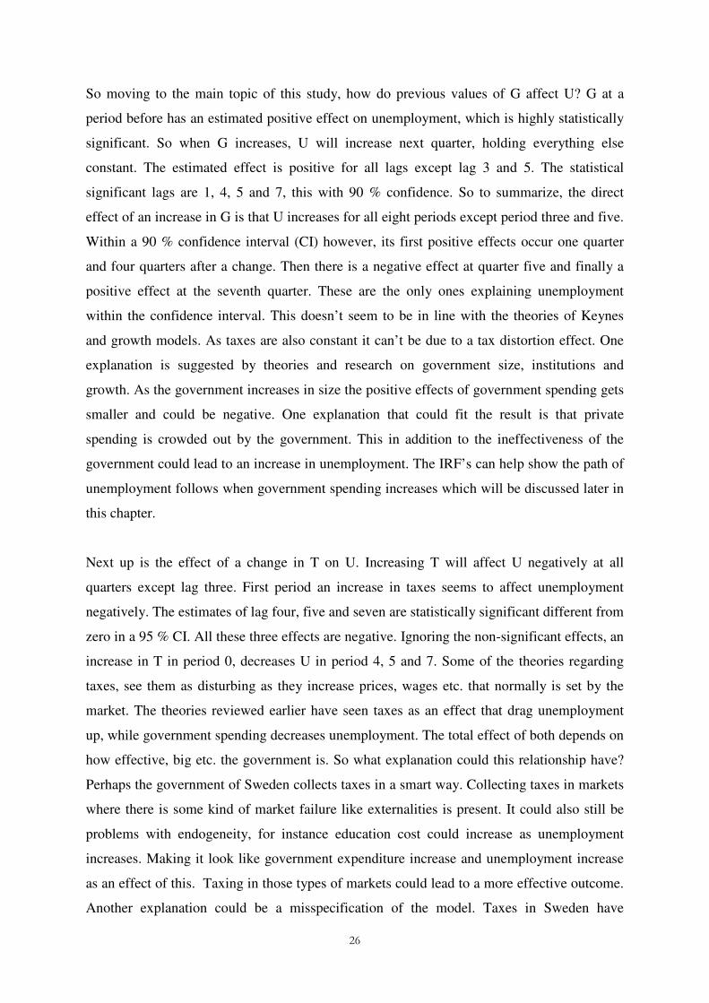
4.6.1 Impulse response functions
To get a better oversight over the effects of a change in government spending and taxes the
impulse response function will be at great service. Figure 4.1 shows the IRF with a 95 % CI
how U change when G increases by one unit. Both G and U is the first difference of
logarithmic value. The figure shows that U increases when G increases. In the first period the
increase is within the 95 % CI so statistically it is a significant increase. In period 2 there is
nearly no effect. In period 3 there is a small decrease. Statistically it can’t be said whether the
total effect is positive or negative for period 2 and 3 given a 95 % confidence. In period 4 one
year after the change in government spending there is an increase in U given the estimated
coefficients. In period 5 there is a very small non-significant increase. In period 6 it is quite
large increase and statistically significant increase. In period 7 and forward the effect is non
or slightly negative.
Figure 4.1 – Impulse response in U to change in G
Figure 4.1 shows the effect for each period. The cumulative response for U is show in figure
4.2. The cumulative response shows the result when all the effects are added through time.
The figure shows that U increases quite steady until it settles down in the 6 quarter. This can
be interpreted as when the G increases with 1, U starts to increase and settles down around a
1 unit increase after 6 quarters. This would mean that if the government increases the growth
rate of spending, this would increase the unemployment growth rate with just as much. It
could also be a cause of reversed causality or endogeneity problem. As earlier discussed,

29
unemployment could make education costs to increase. However looking at a 95 % CI
indicates that the effects is either gone around the 9th quarter or that it continue to increase
and settles down around two. Looking at the cumulative response it indicates that the
increase in U is significant for 9 periods.
Figure 4.2- Cumulative response of U to a change in G.
Figure 4.3 shows the response path of Y when G increases. The effect seems to be negative
for all quarters the first year. Then there is an increase in Y for all periods until the 10th
quarter. After period 10 the effect seems to be gone and there is no longer any effect on
output. The effect of period 10 is the only one that is statistically significant.
Figure 4.3 – Impulse response of Y after a change in G.

30
Figure 4.4 – Cumulative impulse response of Y after a change in G.
Figure 4.4 is the cumulative response of Y after a change in G. Looking at the figure, it is
clear that during first quarters it decreases Y more and more, then start to increase until
period 10 when the cumulative effect is positive. After period 10 it starts dropping towards
zero. First of all it is not a statistically significant effect. Secondly it is a very small effect.
Remember the cumulative IRF of U in response to G. There a 1 unit increase in G settled
with a 1 unit increase of U. Here a 1 unit increase of G increases/decreases Y with 0.1 at
most. What could explain this behaviour? In chapter 3 there was a short discussion about a
scenario where instead of producing more when government demand increased, the producers
started rationing there supply, or that government spending crowds out private investments.
One interesting fact is that G and r has a strong statistical relationship. Looking at the
estimates it looks as G increases r at nearly all quarters until the 5th. After the 5th quarter it
decreases r. The relationship between r and G is statistically significant (within a 95 % CI for
all lags.) This in itself is interesting. That the interest rate increases however suggests that
investing should get more expensive and that may be a reason for output to fall at first.
Increasing r should however lower the relative price of labour if wage is constant and
therefore make it relatively cheaper to hire labour. Unfortunately real wage were not included
in the model, the omission of this variable makes it impossible to know which path it takes.
The real business cycle model suggests that it would decrease. This is also a reason why
unemployment should decrease when government spending increases. That output falls at
first suggests theoretically that unemployment should decrease at first.
31
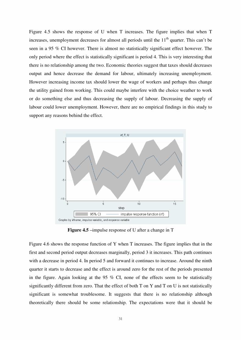
Figure 4.5 shows the response of U when T increases. The figure implies that when T
increases, unemployment decreases for almost all periods until the 11th quarter. This can’t be
seen in a 95 % CI however. There is almost no statistically significant effect however. The
only period where the effect is statistically significant is period 4. This is very interesting that
there is no relationship among the two. Economic theories suggest that taxes should decreases
output and hence decrease the demand for labour, ultimately increasing unemployment.
However increasing income tax should lower the wage of workers and perhaps thus change
the utility gained from working. This could maybe interfere with the choice weather to work
or do something else and thus decreasing the supply of labour. Decreasing the supply of
labour could lower unemployment. However, there are no empirical findings in this study to
support any reasons behind the effect.
Figure 4.5 –impulse response of U after a change in T
Figure 4.6 shows the response function of Y when T increases. The figure implies that in the
first and second period output decreases marginally, period 3 it increases. This path continues
with a decrease in period 4. In period 5 and forward it continues to increase. Around the ninth
quarter it starts to decrease and the effect is around zero for the rest of the periods presented
in the figure. Again looking at the 95 % CI, none of the effects seem to be statistically
significantly different from zero. That the effect of both T on Y and T on U is not statistically
significant is somewhat troublesome. It suggests that there is no relationship although
theoretically there should be some relationship. The expectations were that it should be

32
negative, considering earlier research. That there is no correlation could be because there are
some problems with the model.
Figure 4.6 – Impulse response of Y after a change in T
4.7 Post estimation tests
In this section several post estimation tests are presented. First a Granger causality test to see
if the variables Granger cause one another. Then a lag-order autocorrelation test and finally a
stability condition test.
4.7.1 Wald-Granger causality
The Granger causality test (Granger,1969) can be used to test if lagged values of one variable
can be used to predict another variable. If past values of Xt can be used to predict Yt it is said
that X Granger causes Y. It should however be emphasised that there is some difference
between the classical meaning of causality and Granger causality. That one variable Granger
causes another does not imply causality. Table 4.4 shows the estimation result of a Granger
causality Wald test on unemployment and output. For complete Granger causality test on all
variables see Appendix C. The null hypothesis is that one variable does not Granger cause the
dependent variable while keeping the others constant. The dependent variable is denoted as
“Equation” in the table, while the variable being tested for “non Granger causality” is
denoted excluded. For unemployment all the variables by themselves except r can reject the
null hypothesis of non-Granger causality. The variables all together also explain the value of

33
U. Hence for instance government spending can be said to Granger cause unemployment. To
clarify this means that past values of government spending can be used to predict
unemployment. For output all the variables can be used for prediction. All variables together
also Granger causes Y. For government spending, taxes and unemployment the null-
hypothesis can also be rejected hence there is statistically significant Granger causality. See
appendix C for the complete results of these tests. In appendix C one can see that U also
affects G. This indicates that there is still some problems with reversed causality even thou
transfers is withdrawn from government expenditure. So with this in mind no conclusions can
be drawn wheatear expenditure causes unemployment to rise or if it’s the other way around.
It could of course be that they both effect each other at the same time. The same problem is
present for U and T.
Table 4.4. Granger causality Wald test
Equation Exluded Chi2 Df Prob>chi2
U G 32.802 7 0.000 Y 20.153 7 0.005 r 12.478 7 0.086 T 14.619 7 0.041 ALL 165.81 28 0.000 Y G 57.541 7 0.000 U 47.491 7 0.000 r 40.599 7 0.000 T 40.11 7 0.000 ALL 114.62 28 0.000
4.7.2 Test for autocorrelation
Testing for residual autocorrelation may be done in several ways. The test used in this study
is a Lagrange-multiplier test suggested by Johansen (1995). Other test available to check for
autocorrelation is Breusch-Godfrey test and Portmanteu test, the adjusted portmanteau
statistics have potentially superior small sample properties. (Lütkepohl, 2004). However the
Johansen test has been used as it is included in “STATA” software package. The equation
4.14 describes the formula for the Johansen LM test StataCorp, 2011).
�rs � K � U � 0.5�ln�| ∑ x|∑ y7 ! (4.14)

34
∑ is the variance-covariance matrix of the disturbances from the VAR. ∑ x is the maximum
likelihood estimate of ∑ while∑ z7 is the maximum likelihood estimate of ∑ from a
augmented VAR. The augmented VAR is derived following the method of Davidson and
MacKinnon(1993, p 358). “T” is the number of observations and “d” is the number of
coefficients estimated in the augmented VAR. The asymptotic distribution is {O with K2
degrees of freedom. (StataCorp, 2011)
Table 4.5 Lagrange-multiplier test
Lag Chi2 Df Prob >chi2
1 20.5458 25 0.71764 2 20.7920 25 0.70415
H0: no autocorrelation at lag order
Table 4.5 shows that the null hypothesis cannot be rejected and thus it can be rejected that
there is autocorrelation at lag order 1 and 2.
4.7.3 Stability test
The result of the test can be seen in Appendix C. The estimated values is said to be stable if
all the eigenvalues is inside the unit circle or are strictly less than one. (Fernández-Villaverde
et al, 2007) The stability test result is that all the eigenvalues is inside the unit circle and thus
the estimated model is stable.
4.7.4 Jarque-Bera test
The Jarque-Bera Lagrange multiplier test is a test to determine whether a univariate sample of
T data points or estimated residuals are drawn from a normal distribution. It is a joint test
with the null hypothesis being that there is normality or more precisely that the skewness
equals 0 and the sample kurtosis equals 3. The null is rejected when equation 4.15 exceed the
critical value taken from the asymptotic {O distribution. (Lawford. S, 2005) (Jarque and Bera
1980, 1987)
LM � ~� ��b�
�i�O � �i @�iP �~{O (4.15)
Table 4.6 shows the result of a Jarque-Bera test, the single-equation results are from test
against the null hypothesis that the disturbance for the particular equation is normally

35
distributed. The result for “ALL” the equations are a test against the null that the K
disturbance follows a K-dimensional multivariate normal disturbance. (StataCorp. 2011)
StataCorp (2011) writes that “Failure to reject the null hypothesis indicates a lack of model
misspecification”. Given a 90 % CI the result indicates problems for the equations of G, U
and T. This indicates that there is some misspecification in the estimated model. The test is
sensitive to outliers and small samples. The consequences of violating the assumption of
normality have been heavily studied. The OLS estimators which are efficient under normality
may be sensitive to long-tailed distributions. Test for heteroskedasticity and serial
independence may result in incorrect conclusions. It may also lead to the use of suboptimal
estimators. (Jarque and Bera, 1987)
Table 4.6. Results of Jarque-Bera test Equation Chi2 Df Prob>chi2
G 0.172 2 0.91781 U 0.473 2 0.78923 Y 0.346 2 0.84132 r 5.775 2 0.05572 T 11.890 2 0.00262 ALL 18.656 10 0.04486
5. Conclusions
The aim of this research was to see what effect a change in government spending had on
unemployment. Because of unit-roots many variables were expressed as the first difference of
the logarithmic value the result section has focused more on the sign of the effect rather than
the exact values. This also had the effect that the variables were expressed as growth rates.
This led the interpretation and conclusions from the result to differ from the first intentions.
Instead of seeing the effect that increased government spending have on unemployment, the
result reflects the effects an increased growth rate of government spending has. Even though
most estimates in the 95 % CI can’t be distinguished as positive or negative the IRF and
especially the cumulative IRF indicates that an increase in G would increase U. The
cumulative effect is positive in a 95 % CI until around two years after the first change in G.
This result is in contradiction to what many other VAR studies have found. Other than VAR
country specific studies have had problems finding any statistical significant effect in
Sweden. Cross-country studies however suggest that increased government size would
36
decrease output. This is more similar to the findings of this study. The cumulative effects on
Y after a change in G, were that at first five quarters it would decrease then it would be
increasing for a couple of quarters and finally go towards no effect. These were not
statistically significant which points towards that there is no effect on Y. Looking past the
statistical significance, if there is any effect, it is only in a short time as it goes towards zero
as time increases. An explanation to these effects on unemployment and output could be that
it is because Sweden could be considered having a large government. Increased spending in a
large government offers little or no positive effect on output according to the latest
institutional and governments theories. Another easy explanation could be that government
spending crowds out private spending. One interesting finding was that r depends strongly on
the past values of G. Increasing G would increase r. This effect was statistically significant
for all lags of G. This would make borrowing money more expensive and thus it could lead to
a fall in private investments. Findings indicate that statistically T has no relationship with U
or Y. A decrease in taxes has been found to increase output even more than an increase in
government spending by earlier studies. The result of this study however points in another
direction.
So is there any good explanation why the findings of this study agree with neither classical
economic theory nor the findings of other researchers? As post-estimation test shows there
are problems with non-normality that could generate the use of suboptimal estimators. This is
a problem not only for T but for several of the variables. This test is also sensitive to small
sample sizes, and unfortunately not only for the post test but also for the estimation the
sample used were limited. A change in definition of the national accounts was conducted in
1993 and a reform of the interest rate was done at 1994. This limited the data perhaps too
much. VAR studies lack abilities in explaining the causality and are therefore not optimal for
policy recommendations. Granger causality test were conducted and it was found that
government spending and taxes Granger cause unemployment. This means that lagged values
of government spending and taxes can be used to predict the value of unemployment.
Government spending and taxes did also Granger cause output. This was somewhat
surprising as there isn’t much statistical significance in the estimates. There is a possibility
that the non-normality affected the Granger causality tests.

37
The Granger causality test also shows that G and T is granger caused by U. This indicates
problems with reversed causality and it could still be problems with endogeneity or automatic
stabilizers. As education is highly financed by the public sector in Sweden, perhaps it could
be that it increases when unemployment increases. There are discussions about this and that
higher education in Sweden is just a substitute for many people to avoid unemployment.
Whatever reason is behind this reversed causality it generates problem to draw conclusions.
Not knowing if expenditure effects unemployment or if it is the other way around. One can
only say that there is correlation and not causation.
Policy recommendations would be to lower government spending if one were to decrease
unemployment since this hade a significant effect for at least 9 quarters. However having in
mind that VAR doesn’t explain the cause and that much of the findings weren’t statistically
significant, It’s not recommended to take such actions,. The primary recommendation of this
study would be rather to do further empirical research in the field. In the last years there are
many different theories and empirical findings on what effect governments have on output
and growth but there is not equally much research done on unemployment.

38
References
Abdiweli. A. M. (2003) Institutional differences as source of growth differences. Atlantic
Economic Journal. Vol. 31, No. 4, pp. 348-362.
Agell. J, Ohlsson. H. and Skogman Thoursie. P. (2006) Growth effects of government
expenditure and taxation in rich countries: a comment. European Economic Review. Vol. 50,
No. 1, pp. 211-219
Barro . R. J (1990) Government spending in a simple model of endogenous growth. The
Journal of Political Economy. Vol. 98, No. 5, pp. 103-125
Bergh. A and Henrekson. M (2011) Government size and growth: A survey and interpretation
of the evidence. Journal of Economic Surveys. Vol. 25, No 5, pp.872- 897
Bergh. A and Örhn. N (2011) Growth effects of fiscal policies: a critical appraisal of
Colombier’s study. IFN Working paper858. Research institute of industrial economics,
Stockholm
Blanchard. O, Perotti R (2009) An empirical characterization of the dynamic effect of
changes in government spending and taxes on output. Quarterly Journal of Economics. Vol.
117, no. 4, pp.1329-1368
Burnside. C, Eichenbaum M and Fisher J.D.M (2004) Fiscal shocks and their consequences
Journal of Economic Theory. Vol 115, No. 1, pp. 89-117
Campbell. J. Y (1994) Inspecting the mechanism: An analytical approach to the stochastic
growth model. Journal of Monetary Economics. Vol. 33, No.3, pp. 847- 875
Colombier. C (2009) Growth effects of fiscal policies: an application of robust modified M-
estimators. Applied Economics. Vol. 41, No. 7, pp. 899-912
Dar. A.A and AmirKhalkhali. S (2002) Government size, factor accumulation, and economic
growth: evidence from OECD countries. Journal of Policy Modeling. Vol. 24, No. 7-8. pp.
679-692.

39
Davidson. R and MacKinnon. J.G. (1993) Estimation and inference in econometrics. Oxford:
Oxford University Press.
de Castro. F and Hernándes de Cos. P (2008) the economic effects of fiscal policy: the case of
Spain. Journal of Macroeconomics. Vol 30. No. 3, pp. 1005-1028
Dickey. D. A and Fuller. W.A (1979) Distribution of the estimator for autoregressive Time
Series with a Unit Root. Journal of American Statistical Association, Vol. 74, No 366. pp.
427-31
Dimand. R.W (2008) Edmund Phelps and Modern Macroeconomics. Review of Political
Economy. Vol. 20, No. 1, pp. 23-39
Edelberg. W, Eichenbaum M and Fisher J.D.M (1999) Understanding the effects of a shock
to government purchases. Review of Economic Dynamics. Vol. 2, No 1, pp. 166-206
Elliot. G, Rothenberg. T. J and Stock. J. H. (1996) Efficient Test for an autoregressive Unit
Root, Econometrica, Vol. 64. No 4. pp. 813-836
Fernández-Villaverde. J, Rubio-Ramírez. J. F, Sargent T. J and Watson. M. W (2007) ABCs
(and Ds) of Understanding VARs, American Economic Review, Vol. 97. No. 3
pp. 1021-1026
Fregert, K. and Jonung, L. (2005). Makroekonomi: teori, politik och institutioner. 2 ed. Lund:
Studentlitteratur
Fölster. S and Henrekson. M (2001) Growth effects of government expenditure and taxation
in rich countries. European Economic Review. Vol. 45, No 8, pp. 1501-1520
Granger. C. W. J (1969) Investigating causal relations by econometric models and cross-
spectral methods. Econometrica. Vol. 37, No. 3, pp. 424-38.
Hannan. E. J, Quinn. B. G. (1979) The determination of the order of an autoregression Journal of the Royal Statistical Society, Series B, 41 pp. 190–195
40
Jarque. C. M and Bera. A.K . 1980 . Efficient tests for normality, homoscedasticity and serial
independence of regression residuals . Economics Letters , Vol. 6, pp. 255 – 259
Jarque. C.M and Bera. A.K . 1987 . A test for normality of observations and regression
residuals. International Statistical Review. Vol. 55, pp. 163 – 172 .
Johansen. S. (1995) Likelihood-Based Inference on Cointegrated Vector Auto-Regressive
Models. Oxford: Oxford University Press.
Lane. P. R and Tornell. A. (1996) Power, Growth and the Voracity Effect. Journal of
Economic Growth. Vol. 1, No. 2, pp. 213-241
Lawford. S (2005) Finite-sample quantiles of the Jarque-Bera test. Applied Economics
Letters. Vol. 12, No. 6, pp 351-354.
Lütkepohl. H (2005). New introduction to multiple time series analysis, New York: Soringer.
Mankiw. N. G (1995) The growth of nations. Brookings paper on Economic activity, (1), pp
275-326
Mankiw, N. G. and Taylor, M. P. (2007). Macroeconomics. European ed. New York: Worth
Mountford. A and Uhlig. H (2009) What are the effects of fiscal policy shocks? Journal of
Applied Econometrics. Vol. 24, No 6, pp. 960- 992
North. D (1990). Institutions, Institutional change and Economic performance. New York:
Cambridge University press
Ramey. V. A and Shapiro. M. D (1998) Costly capital reallocation and the effects of
government spending. Carnegie-Rochester conference series on public policy. Vol. 48, No. 1
pp. 145-194

41
Rodrik. D., Subramanian, A. and Trebbi. F. (2004) Intitutions rule: the primacy of institutions
over geography and integration in economic development. Journal of Economic Growth. Vol.
9, No. 2, pp. 131-165.
Romer. C. D and Romer. D. H (2010) The macroeconomic effects of tax changes: Estimates
based on a new measure of fiscal shocks. American Economic Review. Vol. 100, No. 3, pp
763-801
Romer. D. H (2012) Advanced macroeconomics. 4 ed. New York: McGraw-Hill
Romer. P. M (1986) Increasing returns and long-run growth. The Journal of Political
Economy. Vol. 94, No. 5, pp. 1002-1037
Satya. P (1996) Defence spending and unemployment rates: An empirical analysis for the
OECD. Journal of Economic Studies. Vol. 23, No 2, pp. 44-54
Schwarz. G (1978) Estimating the dimension of a model. The Annals of Statistics. Vol. 6,
No.2, pp 461-464
Sims. C.A (1980) Macroeconomics and Reality. Econometrica. Vol. 48, No. 1, pp. 1-48.
Slemrod. J. (1995) What do cross-country studies teach about government involvement,
prosperity, and economic growth? Brookings Papers on Economic Activity (1), pp 373-431
Solow. R. M (1956) A contribution to the theory of economic growth. Quarterly Journal of
Economics. Vol. 70, No. 1, pp. 65-94
Statacorp. (2011) Stata Statistical software: Release 12. College Station, TX: StataCorp LP.
Verbeek, M (2012). A guide to modern econometrics. 4. ed. Hoboken, NJ: Wiley
Young. P. C and Pedregal D.J (1999) Macro-economic relativity: government spending,
private investment and unemployment in the USA 1948–1998. Structural Change and
Economic Dynamics. Vol. 10, No 3-4, pp. 359-380.

42
Appendix A
DF-GLS for G (logarithmic value) Number of obs = 62 Maxlag = 11 chosen by Schwert criterion DF-GLS tau 1% Critical 5% Critical 10% Critical [lags] Test Statistic Value Value Value ------------------------------------------------------------------------------ 11 -1.217 -3.679 -2.715 -2.439 10 -1.177 -3.679 -2.758 -2.482 9 -1.182 -3.679 -2.803 -2.526 8 -1.651 -3.679 -2.848 -2.569 7 -1.307 -3.679 -2.892 -2.611 6 -1.586 -3.679 -2.935 -2.652 5 -2.032 -3.679 -2.976 -2.690 4 -2.358 -3.679 -3.015 -2.726 3 -0.731 -3.679 -3.050 -2.759 2 -1.987 -3.679 -3.083 -2.789 1 -2.074 -3.679 -3.110 -2.814 Opt Lag (Ng-Perron seq t) = 4 with RMSE .0562896 Min SC = -5.421657 at lag 4 with RMSE .0562896 Min MAIC = -5.475809 at lag 9 with RMSE .0526119 DF-GLS for G (first diffrence) Number of obs = 61 Maxlag = 11 chosen by Schwert criterion DF-GLS tau 1% Critical 5% Critical 10% Critical [lags] Test Statistic Value Value Value ------------------------------------------------------------------------------ 11 -1.810 -3.683 -2.711 -2.435 10 -2.547 -3.683 -2.756 -2.479 9 -2.816 -3.683 -2.801 -2.523 8 -3.113 -3.683 -2.846 -2.567 7 -2.690 -3.683 -2.891 -2.610 6 -3.453 -3.683 -2.935 -2.652 5 -3.294 -3.683 -2.977 -2.691 4 -2.899 -3.683 -3.016 -2.728 3 -2.660 -3.683 -3.053 -2.762 2 -10.129 -3.683 -3.086 -2.792 1 -7.021 -3.683 -3.114 -2.818 Opt Lag (Ng-Perron seq t) = 11 with RMSE .0507709 Min SC = -5.373897 at lag 3 with RMSE .0595028 Min MAIC = -.6637253 at lag 3 with RMSE .0595028

43
DF-GLS for Y (logarithmic value) Number of obs = 67 Maxlag = 11 chosen by Schwert criterion DF-GLS tau 1% Critical 5% Critical 10% Critical [lags] Test Statistic Value Value Value ------------------------------------------------------------------------------ 11 -1.096 -3.660 -2.731 -2.456 10 -1.410 -3.660 -2.772 -2.496 9 -1.538 -3.660 -2.813 -2.536 8 -1.493 -3.660 -2.854 -2.576 7 -1.482 -3.660 -2.894 -2.614 6 -1.426 -3.660 -2.933 -2.651 5 -1.485 -3.660 -2.971 -2.686 4 -1.810 -3.660 -3.006 -2.718 3 -2.569 -3.660 -3.038 -2.748 2 -2.124 -3.660 -3.067 -2.774 1 -1.698 -3.660 -3.093 -2.797 Opt Lag (Ng-Perron seq t) = 4 with RMSE .0082792 Min SC = -9.286238 at lag 1 with RMSE .009042 Min MAIC = -9.35625 at lag 5 with RMSE .0081971 DF-GLS for Y ( First difference) Number of obs = 61 Maxlag = 11 chosen by Schwert criterion DF-GLS tau 1% Critical 5% Critical 10% Critical [lags] Test Statistic Value Value Value ------------------------------------------------------------------------------ 11 -2.782 -3.683 -2.711 -2.435 10 -3.466 -3.683 -2.756 -2.479 9 -3.021 -3.683 -2.801 -2.523 8 -2.836 -3.683 -2.846 -2.567 7 -3.087 -3.683 -2.891 -2.610 6 -3.357 -3.683 -2.935 -2.652 5 -3.879 -3.683 -2.977 -2.691 4 -4.228 -3.683 -3.016 -2.728 3 -4.018 -3.683 -3.053 -2.762 2 -3.010 -3.683 -3.086 -2.792 1 -3.760 -3.683 -3.114 -2.818 Opt Lag (Ng-Perron seq t) = 3 with RMSE .0085629 Min SC = -9.251066 at lag 3 with RMSE .0085629 Min MAIC = -8.741276 at lag 2 with RMSE .009154 DF-GLS for r Number of obs = 62 Maxlag = 11 chosen by Schwert criterion DF-GLS tau 1% Critical 5% Critical 10% Critical [lags] Test Statistic Value Value Value ------------------------------------------------------------------------------ 11 -3.178 -3.679 -2.715 -2.439 10 -2.843 -3.679 -2.758 -2.482 9 -2.603 -3.679 -2.803 -2.526 8 -2.617 -3.679 -2.848 -2.569 7 -3.047 -3.679 -2.892 -2.611 6 -2.554 -3.679 -2.935 -2.652 5 -2.507 -3.679 -2.976 -2.690 4 -3.105 -3.679 -3.015 -2.726 3 -4.303 -3.679 -3.050 -2.759 2 -3.392 -3.679 -3.083 -2.789 1 -3.557 -3.679 -3.110 -2.814 Opt Lag (Ng-Perron seq t) = 7 with RMSE .785679

44
DF-GLS for r (first difference) Number of obs = 61 Maxlag = 11 chosen by Schwert criterion DF-GLS tau 1% Critical 5% Critical 10% Critical [lags] Test Statistic Value Value Value ------------------------------------------------------------------------------ 11 -2.321 -3.683 -2.711 -2.435 10 -1.970 -3.683 -2.756 -2.479 9 -2.253 -3.683 -2.801 -2.523 8 -2.652 -3.683 -2.846 -2.567 7 -2.967 -3.683 -2.891 -2.610 6 -2.830 -3.683 -2.935 -2.652 5 -3.811 -3.683 -2.977 -2.691 4 -5.045 -3.683 -3.016 -2.728 3 -5.058 -3.683 -3.053 -2.762 2 -4.153 -3.683 -3.086 -2.792 1 -6.151 -3.683 -3.114 -2.818 Opt Lag (Ng-Perron seq t) = 11 with RMSE .8178242 Min SC = .1487767 at lag 3 with RMSE .9413932 Min MAIC = 1.670067 at lag 10 with RMSE .842382 DF-GLS for U (logarithmic value) Number of obs = 62 Maxlag = 11 chosen by Schwert criterion DF-GLS tau 1% Critical 5% Critical 10% Critical [lags] Test Statistic Value Value Value ------------------------------------------------------------------------------ 11 -1.722 -3.679 -2.715 -2.439 10 -1.637 -3.679 -2.758 -2.482 9 -1.533 -3.679 -2.803 -2.526 8 -1.605 -3.679 -2.848 -2.569 7 -1.974 -3.679 -2.892 -2.611 6 -2.015 -3.679 -2.935 -2.652 5 -1.983 -3.679 -2.976 -2.690 4 -2.000 -3.679 -3.015 -2.726 3 -2.361 -3.679 -3.050 -2.759 2 -1.796 -3.679 -3.083 -2.789 1 -1.432 -3.679 -3.110 -2.814 Opt Lag (Ng-Perron seq t) = 3 with RMSE .3720859 Min SC = -1.710994 at lag 3 with RMSE .3720859 Min MAIC = -1.711462 at lag 1 with RMSE .4036893 DF-GLS for U (first difference) Number of obs = 61 Maxlag = 11 chosen by Schwert criterion DF-GLS tau 1% Critical 5% Critical 10% Critical [lags] Test Statistic Value Value Value ------------------------------------------------------------------------------ 11 -2.137 -3.683 -2.711 -2.435 10 -2.468 -3.683 -2.756 -2.479 9 -2.843 -3.683 -2.801 -2.523 8 -3.146 -3.683 -2.846 -2.567 7 -3.119 -3.683 -2.891 -2.610 6 -2.609 -3.683 -2.935 -2.652 5 -2.678 -3.683 -2.977 -2.691 4 -2.948 -3.683 -3.016 -2.728 3 -3.111 -3.683 -3.053 -2.762 2 -2.878 -3.683 -3.086 -2.792 1 -4.375 -3.683 -3.114 -2.818 Opt Lag (Ng-Perron seq t) = 7 with RMSE .0528585

45
DF-GLS for T (logarithmic value) Number of obs = 62 Maxlag = 11 chosen by Schwert criterion DF-GLS tau 1% Critical 5% Critical 10% Critical [lags] Test Statistic Value Value Value ------------------------------------------------------------------------------ 11 -1.354 -3.679 -2.715 -2.439 10 -1.470 -3.679 -2.758 -2.482 9 -1.487 -3.679 -2.803 -2.526 8 -1.284 -3.679 -2.848 -2.569 7 -1.272 -3.679 -2.892 -2.611 6 -1.309 -3.679 -2.935 -2.652 5 -1.438 -3.679 -2.976 -2.690 4 -1.751 -3.679 -3.015 -2.726 3 -2.206 -3.679 -3.050 -2.759 2 -1.797 -3.679 -3.083 -2.789 1 -1.392 -3.679 -3.110 -2.814 Opt Lag (Ng-Perron seq t) = 2 with RMSE .0098335 Min SC = -9.055028 at lag 1 with RMSE .0101115 Min MAIC = -9.089125 at lag 1 with RMSE .0101115 DF-GLS for T (first difference) Number of obs = 61 Maxlag = 11 chosen by Schwert criterion DF-GLS tau 1% Critical 5% Critical 10% Critical [lags] Test Statistic Value Value Value ------------------------------------------------------------------------------ 11 -2.659 -3.683 -2.711 -2.435 10 -2.858 -3.683 -2.756 -2.479 9 -2.720 -3.683 -2.801 -2.523 8 -2.771 -3.683 -2.846 -2.567 7 -3.247 -3.683 -2.891 -2.610 6 -3.563 -3.683 -2.935 -2.652 5 -3.844 -3.683 -2.977 -2.691 4 -3.907 -3.683 -3.016 -2.728 3 -3.552 -3.683 -3.053 -2.762 2 -3.061 -3.683 -3.086 -2.792 1 -3.955 -3.683 -3.114 -2.818 Opt Lag (Ng-Perron seq t) = 3 with RMSE .0097227 Min SC = -9.061631 at lag 1 with RMSE .0100699 Min MAIC = -8.491998 at lag 2 with RMSE .0099859

46
Appendix B
Vector autoregression
Sample: 1996q2 - 2012q3 No. of obs = 66
Log likelihood = 823.6543 AIC = -18.89861
FPE = 1.12e-14 HQIC = -16.27668
Det(Sigma_ml) = 9.95e-18 SBIC = -12.2633
Equation Parms RMSE R-sq chi2 P>chi2
----------------------------------------------------------------
U 40 .043424 0.7721 223.6013 0.0000
G 40 .063986 0.8728 452.9846 0.0000
T 40 .008158 0.7642 213.9412 0.0000
Y 40 .007934 0.7480 195.8787 0.0000
r 40 .753847 0.7687 219.3794 0.0000
----------------------------------------------------------------
------------------------------------------------------------------------------
| Coef. Std. Err. z P>|z| [95% Conf. Interval]
-------------+----------------------------------------------------------------
U |
U |
L1. | -.1780452 .1313488 -1.36 0.175 -.4354841 .0793937
L2. | .0777276 .166357 0.47 0.640 -.2483261 .4037813
L3. | -.0055225 .1281513 -0.04 0.966 -.2566943 .2456493
L4. | -.2223524 .1101709 -2.02 0.044 -.4382835 -.0064214
L5. | -.0189059 .10992 -0.17 0.863 -.2343453 .1965334
L6. | .0073134 .1108759 0.07 0.947 -.2099994 .2246262
L7. | .1897611 .0998768 1.90 0.057 -.0059938 .3855159
|
G |
L1. | .3754411 .0887044 4.23 0.000 .2015838 .5492985
L2. | .0831741 .1070204 0.78 0.437 -.126582 .2929302
L3. | -.0664125 .0939658 -0.71 0.480 -.2505821 .1177572
L4. | .1418595 .0841294 1.69 0.092 -.0230311 .3067501
L5. | -.35168 .103787 -3.39 0.001 -.5550987 -.1482612
L6. | .087011 .1190693 0.73 0.465 -.1463605 .3203824
L7. | .2743048 .1102839 2.49 0.013 .0581523 .4904574
|
T |
L1. | -2.501389 2.083388 -1.20 0.230 -6.584754 1.581976
L2. | -2.126716 1.762134 -1.21 0.227 -5.580435 1.327003
L3. | 2.482996 1.694608 1.47 0.143 -.8383759 5.804367
L4. | -4.217641 1.850905 -2.28 0.023 -7.845349 -.5899333
L5. | -3.477796 1.540112 -2.26 0.024 -6.49636 -.4592315
L6. | -1.434258 1.698253 -0.84 0.398 -4.762772 1.894256
L7. | -3.598767 1.667679 -2.16 0.031 -6.867358 -.3301753
|
Y |
L1. | -3.993323 2.160207 -1.85 0.065 -8.22725 .240605
L2. | -3.714115 1.920013 -1.93 0.053 -7.477272 .0490425
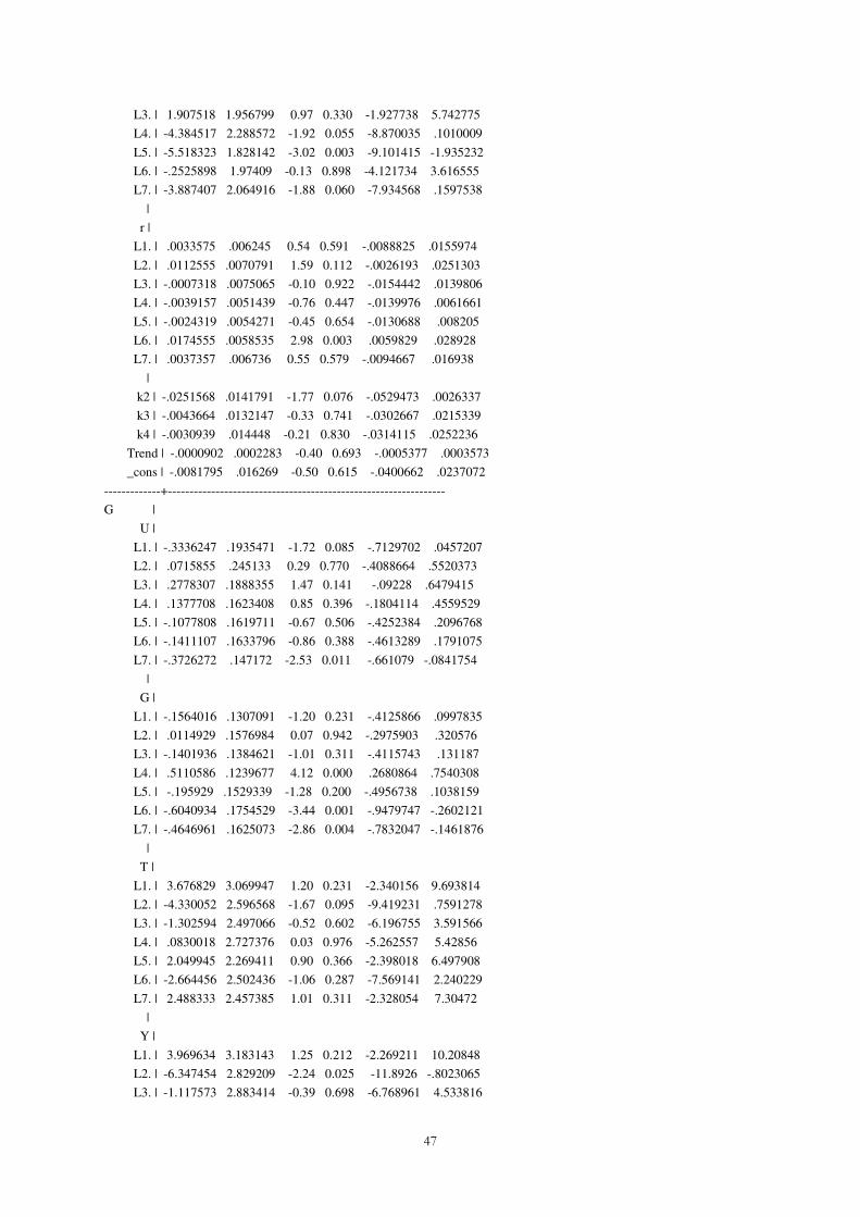
47
L3. | 1.907518 1.956799 0.97 0.330 -1.927738 5.742775
L4. | -4.384517 2.288572 -1.92 0.055 -8.870035 .1010009
L5. | -5.518323 1.828142 -3.02 0.003 -9.101415 -1.935232
L6. | -.2525898 1.97409 -0.13 0.898 -4.121734 3.616555
L7. | -3.887407 2.064916 -1.88 0.060 -7.934568 .1597538
|
r |
L1. | .0033575 .006245 0.54 0.591 -.0088825 .0155974
L2. | .0112555 .0070791 1.59 0.112 -.0026193 .0251303
L3. | -.0007318 .0075065 -0.10 0.922 -.0154442 .0139806
L4. | -.0039157 .0051439 -0.76 0.447 -.0139976 .0061661
L5. | -.0024319 .0054271 -0.45 0.654 -.0130688 .008205
L6. | .0174555 .0058535 2.98 0.003 .0059829 .028928
L7. | .0037357 .006736 0.55 0.579 -.0094667 .016938
|
k2 | -.0251568 .0141791 -1.77 0.076 -.0529473 .0026337
k3 | -.0043664 .0132147 -0.33 0.741 -.0302667 .0215339
k4 | -.0030939 .014448 -0.21 0.830 -.0314115 .0252236
Trend | -.0000902 .0002283 -0.40 0.693 -.0005377 .0003573
_cons | -.0081795 .016269 -0.50 0.615 -.0400662 .0237072
-------------+----------------------------------------------------------------
G |
U |
L1. | -.3336247 .1935471 -1.72 0.085 -.7129702 .0457207
L2. | .0715855 .245133 0.29 0.770 -.4088664 .5520373
L3. | .2778307 .1888355 1.47 0.141 -.09228 .6479415
L4. | .1377708 .1623408 0.85 0.396 -.1804114 .4559529
L5. | -.1077808 .1619711 -0.67 0.506 -.4252384 .2096768
L6. | -.1411107 .1633796 -0.86 0.388 -.4613289 .1791075
L7. | -.3726272 .147172 -2.53 0.011 -.661079 -.0841754
|
G |
L1. | -.1564016 .1307091 -1.20 0.231 -.4125866 .0997835
L2. | .0114929 .1576984 0.07 0.942 -.2975903 .320576
L3. | -.1401936 .1384621 -1.01 0.311 -.4115743 .131187
L4. | .5110586 .1239677 4.12 0.000 .2680864 .7540308
L5. | -.195929 .1529339 -1.28 0.200 -.4956738 .1038159
L6. | -.6040934 .1754529 -3.44 0.001 -.9479747 -.2602121
L7. | -.4646961 .1625073 -2.86 0.004 -.7832047 -.1461876
|
T |
L1. | 3.676829 3.069947 1.20 0.231 -2.340156 9.693814
L2. | -4.330052 2.596568 -1.67 0.095 -9.419231 .7591278
L3. | -1.302594 2.497066 -0.52 0.602 -6.196755 3.591566
L4. | .0830018 2.727376 0.03 0.976 -5.262557 5.42856
L5. | 2.049945 2.269411 0.90 0.366 -2.398018 6.497908
L6. | -2.664456 2.502436 -1.06 0.287 -7.569141 2.240229
L7. | 2.488333 2.457385 1.01 0.311 -2.328054 7.30472
|
Y |
L1. | 3.969634 3.183143 1.25 0.212 -2.269211 10.20848
L2. | -6.347454 2.829209 -2.24 0.025 -11.8926 -.8023065
L3. | -1.117573 2.883414 -0.39 0.698 -6.768961 4.533816
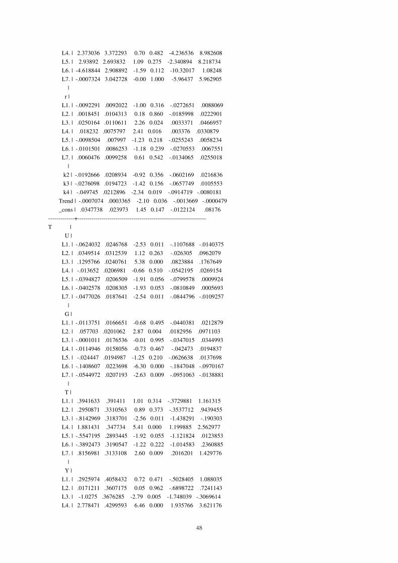
48
L4. | 2.373036 3.372293 0.70 0.482 -4.236536 8.982608
L5. | 2.93892 2.693832 1.09 0.275 -2.340894 8.218734
L6. | -4.618844 2.908892 -1.59 0.112 -10.32017 1.08248
L7. | -.0007324 3.042728 -0.00 1.000 -5.96437 5.962905
|
r |
L1. | -.0092291 .0092022 -1.00 0.316 -.0272651 .0088069
L2. | .0018451 .0104313 0.18 0.860 -.0185998 .0222901
L3. | .0250164 .0110611 2.26 0.024 .0033371 .0466957
L4. | .018232 .0075797 2.41 0.016 .003376 .0330879
L5. | -.0098504 .007997 -1.23 0.218 -.0255243 .0058234
L6. | -.0101501 .0086253 -1.18 0.239 -.0270553 .0067551
L7. | .0060476 .0099258 0.61 0.542 -.0134065 .0255018
|
k2 | -.0192666 .0208934 -0.92 0.356 -.0602169 .0216836
k3 | -.0276098 .0194723 -1.42 0.156 -.0657749 .0105553
k4 | -.049745 .0212896 -2.34 0.019 -.0914719 -.0080181
Trend | -.0007074 .0003365 -2.10 0.036 -.0013669 -.0000479
_cons | .0347738 .023973 1.45 0.147 -.0122124 .08176
-------------+----------------------------------------------------------------
T |
U |
L1. | -.0624032 .0246768 -2.53 0.011 -.1107688 -.0140375
L2. | .0349514 .0312539 1.12 0.263 -.026305 .0962079
L3. | .1295766 .0240761 5.38 0.000 .0823884 .1767649
L4. | -.013652 .0206981 -0.66 0.510 -.0542195 .0269154
L5. | -.0394827 .0206509 -1.91 0.056 -.0799578 .0009924
L6. | -.0402578 .0208305 -1.93 0.053 -.0810849 .0005693
L7. | -.0477026 .0187641 -2.54 0.011 -.0844796 -.0109257
|
G |
L1. | -.0113751 .0166651 -0.68 0.495 -.0440381 .0212879
L2. | .057703 .0201062 2.87 0.004 .0182956 .0971103
L3. | -.0001011 .0176536 -0.01 0.995 -.0347015 .0344993
L4. | -.0114946 .0158056 -0.73 0.467 -.042473 .0194837
L5. | -.024447 .0194987 -1.25 0.210 -.0626638 .0137698
L6. | -.1408607 .0223698 -6.30 0.000 -.1847048 -.0970167
L7. | -.0544972 .0207193 -2.63 0.009 -.0951063 -.0138881
|
T |
L1. | .3941633 .391411 1.01 0.314 -.3729881 1.161315
L2. | .2950871 .3310563 0.89 0.373 -.3537712 .9439455
L3. | -.8142969 .3183701 -2.56 0.011 -1.438291 -.190303
L4. | 1.881431 .347734 5.41 0.000 1.199885 2.562977
L5. | -.5547195 .2893445 -1.92 0.055 -1.121824 .0123853
L6. | -.3892473 .3190547 -1.22 0.222 -1.014583 .2360885
L7. | .8156981 .3133108 2.60 0.009 .2016201 1.429776
|
Y |
L1. | .2925974 .4058432 0.72 0.471 -.5028405 1.088035
L2. | .0171211 .3607175 0.05 0.962 -.6898722 .7241143
L3. | -1.0275 .3676285 -2.79 0.005 -1.748039 -.3069614
L4. | 2.778471 .4299593 6.46 0.000 1.935766 3.621176
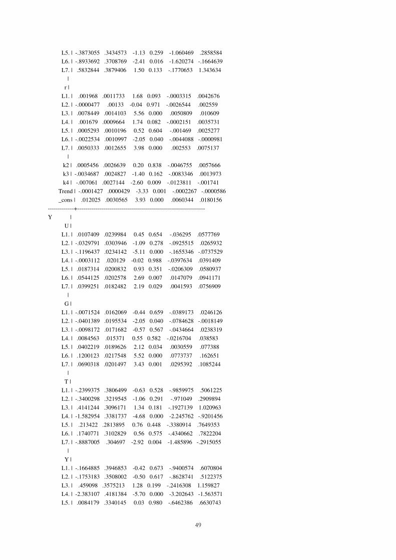
49
L5. | -.3873055 .3434573 -1.13 0.259 -1.060469 .2858584
L6. | -.8933692 .3708769 -2.41 0.016 -1.620274 -.1664639
L7. | .5832844 .3879406 1.50 0.133 -.1770653 1.343634
|
r |
L1. | .001968 .0011733 1.68 0.093 -.0003315 .0042676
L2. | -.0000477 .00133 -0.04 0.971 -.0026544 .002559
L3. | .0078449 .0014103 5.56 0.000 .0050809 .010609
L4. | .001679 .0009664 1.74 0.082 -.0002151 .0035731
L5. | .0005293 .0010196 0.52 0.604 -.001469 .0025277
L6. | -.0022534 .0010997 -2.05 0.040 -.0044088 -.0000981
L7. | .0050333 .0012655 3.98 0.000 .002553 .0075137
|
k2 | .0005456 .0026639 0.20 0.838 -.0046755 .0057666
k3 | -.0034687 .0024827 -1.40 0.162 -.0083346 .0013973
k4 | -.007061 .0027144 -2.60 0.009 -.0123811 -.001741
Trend | -.0001427 .0000429 -3.33 0.001 -.0002267 -.0000586
_cons | .012025 .0030565 3.93 0.000 .0060344 .0180156
-------------+----------------------------------------------------------------
Y |
U |
L1. | .0107409 .0239984 0.45 0.654 -.036295 .0577769
L2. | -.0329791 .0303946 -1.09 0.278 -.0925515 .0265932
L3. | -.1196437 .0234142 -5.11 0.000 -.1655346 -.0737529
L4. | -.0003112 .020129 -0.02 0.988 -.0397634 .0391409
L5. | .0187314 .0200832 0.93 0.351 -.0206309 .0580937
L6. | .0544125 .0202578 2.69 0.007 .0147079 .0941171
L7. | .0399251 .0182482 2.19 0.029 .0041593 .0756909
|
G |
L1. | -.0071524 .0162069 -0.44 0.659 -.0389173 .0246126
L2. | -.0401389 .0195534 -2.05 0.040 -.0784628 -.0018149
L3. | -.0098172 .0171682 -0.57 0.567 -.0434664 .0238319
L4. | .0084563 .015371 0.55 0.582 -.0216704 .038583
L5. | .0402219 .0189626 2.12 0.034 .0030559 .077388
L6. | .1200123 .0217548 5.52 0.000 .0773737 .162651
L7. | .0690318 .0201497 3.43 0.001 .0295392 .1085244
|
T |
L1. | -.2399375 .3806499 -0.63 0.528 -.9859975 .5061225
L2. | -.3400298 .3219545 -1.06 0.291 -.971049 .2909894
L3. | .4141244 .3096171 1.34 0.181 -.1927139 1.020963
L4. | -1.582954 .3381737 -4.68 0.000 -2.245762 -.9201456
L5. | .213422 .2813895 0.76 0.448 -.3380914 .7649353
L6. | .1740771 .3102829 0.56 0.575 -.4340662 .7822204
L7. | -.8887005 .304697 -2.92 0.004 -1.485896 -.2915055
|
Y |
L1. | -.1664885 .3946853 -0.42 0.673 -.9400574 .6070804
L2. | -.1753183 .3508002 -0.50 0.617 -.8628741 .5122375
L3. | .459098 .3575213 1.28 0.199 -.2416308 1.159827
L4. | -2.383107 .4181384 -5.70 0.000 -3.202643 -1.563571
L5. | .0084179 .3340145 0.03 0.980 -.6462386 .6630743

50
L6. | .5792217 .3606803 1.61 0.108 -.1276987 1.286142
L7. | -.6057267 .3772749 -1.61 0.108 -1.345172 .1337186
|
r |
L1. | -.0029387 .001141 -2.58 0.010 -.0051751 -.0007024
L2. | -.0015044 .0012934 -1.16 0.245 -.0040394 .0010307
L3. | -.0079949 .0013715 -5.83 0.000 -.010683 -.0053069
L4. | -.0016926 .0009398 -1.80 0.072 -.0035347 .0001494
L5. | -.0015292 .0009916 -1.54 0.123 -.0034727 .0004142
L6. | .0008393 .0010695 0.78 0.433 -.0012568 .0029354
L7. | -.0042741 .0012307 -3.47 0.001 -.0066863 -.001862
|
k2 | .0017536 .0025906 0.68 0.498 -.0033239 .0068311
k3 | .0040981 .0024144 1.70 0.090 -.000634 .0088303
k4 | .0071034 .0026398 2.69 0.007 .0019295 .0122772
Trend | .0001145 .0000417 2.74 0.006 .0000327 .0001963
_cons | -.0120886 .0029725 -4.07 0.000 -.0179145 -.0062627
-------------+----------------------------------------------------------------
r |
U |
L1. | -5.839341 2.280246 -2.56 0.010 -10.30854 -1.37014
L2. | .5408874 2.887997 0.19 0.851 -5.119482 6.201257
L3. | 4.832589 2.224736 2.17 0.030 .4721858 9.192992
L4. | 5.500454 1.912593 2.88 0.004 1.75184 9.249068
L5. | 6.035761 1.908238 3.16 0.002 2.295683 9.775839
L6. | -2.710812 1.924832 -1.41 0.159 -6.483414 1.06179
L7. | -8.229023 1.733884 -4.75 0.000 -11.62737 -4.830672
|
G |
L1. | -3.933689 1.539929 -2.55 0.011 -6.951894 -.9154839
L2. | 8.046747 1.857899 4.33 0.000 4.405331 11.68816
L3. | 7.158727 1.63127 4.39 0.000 3.961497 10.35596
L4. | 5.054599 1.460506 3.46 0.001 2.192059 7.917139
L5. | 7.155076 1.801767 3.97 0.000 3.623678 10.68647
L6. | -7.137401 2.067071 -3.45 0.001 -11.18879 -3.086016
L7. | -4.636967 1.914555 -2.42 0.015 -8.389427 -.8845077
|
T |
L1. | -20.9183 36.16811 -0.58 0.563 -91.80649 49.96989
L2. | -59.92786 30.59107 -1.96 0.050 -119.8853 .0295242
L3. | -54.90287 29.41881 -1.87 0.062 -112.5627 2.756935
L4. | 41.06962 32.13216 1.28 0.201 -21.90826 104.0475
L5. | -41.17505 26.73671 -1.54 0.124 -93.57805 11.22795
L6. | 44.09307 29.48207 1.50 0.135 -13.69072 101.8769
L7. | 33.39695 28.95131 1.15 0.249 -23.34657 90.14048
|
Y |
L1. | -29.308 37.50171 -0.78 0.435 -102.81 44.19399
L2. | -58.44531 33.33189 -1.75 0.080 -123.7746 6.883999
L3. | -48.0672 33.97051 -1.41 0.157 -114.6482 18.51377
L4. | 116.5341 39.73015 2.93 0.003 38.66443 194.4037
L5. | -33.24382 31.73697 -1.05 0.295 -95.44715 28.9595
L6. | 28.59972 34.27067 0.83 0.404 -38.56956 95.76899
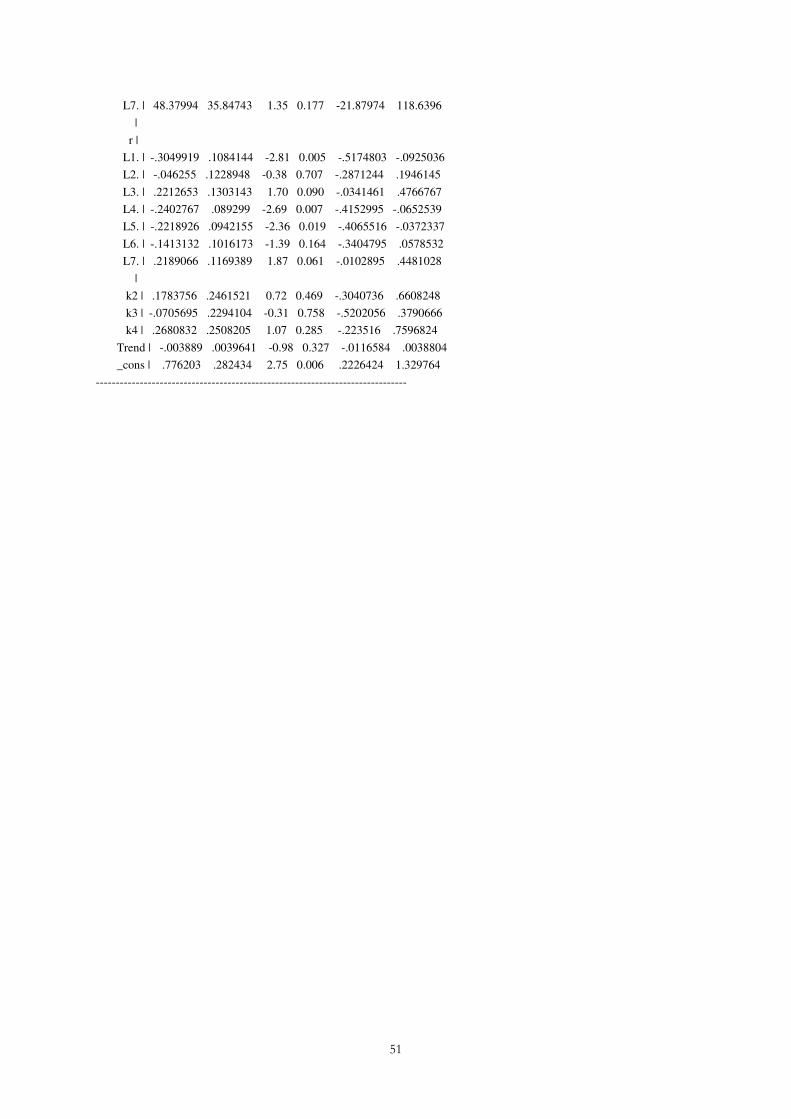
51
L7. | 48.37994 35.84743 1.35 0.177 -21.87974 118.6396
|
r |
L1. | -.3049919 .1084144 -2.81 0.005 -.5174803 -.0925036
L2. | -.046255 .1228948 -0.38 0.707 -.2871244 .1946145
L3. | .2212653 .1303143 1.70 0.090 -.0341461 .4766767
L4. | -.2402767 .089299 -2.69 0.007 -.4152995 -.0652539
L5. | -.2218926 .0942155 -2.36 0.019 -.4065516 -.0372337
L6. | -.1413132 .1016173 -1.39 0.164 -.3404795 .0578532
L7. | .2189066 .1169389 1.87 0.061 -.0102895 .4481028
|
k2 | .1783756 .2461521 0.72 0.469 -.3040736 .6608248
k3 | -.0705695 .2294104 -0.31 0.758 -.5202056 .3790666
k4 | .2680832 .2508205 1.07 0.285 -.223516 .7596824
Trend | -.003889 .0039641 -0.98 0.327 -.0116584 .0038804
_cons | .776203 .282434 2.75 0.006 .2226424 1.329764
------------------------------------------------------------------------------

52
Appendix C
Granger causality Wald tests +------------------------------------------------------------------+ Equation Excluded chi2 df Prob > chi2 --------------------------------------+--------------------------- U G 32.802 7 0.000 U T 14.619 7 0.041 U Y 20.153 7 0.005 U r 12.478 7 0.086 U ALL 165.81 28 0.000 --------------------------------------+--------------------------- G U 14.963 7 0.036 G T 13.109 7 0.069 G Y 14.516 7 0.043 G r 18.313 7 0.011 G ALL 51.245 28 0.005 --------------------------------------+--------------------------- T U 61.052 7 0.000 T G 57.874 7 0.000 T Y 84.23 7 0.000 T r 46.164 7 0.000 T ALL 144.6 28 0.000 --------------------------------------+--------------------------- Y U 47.491 7 0.000 Y G 57.541 7 0.000 Y T 40.11 7 0.000 Y r 40.599 7 0.000 Y ALL 114.62 28 0.000 --------------------------------------+--------------------------- r U 52.816 7 0.000 r G 68.803 7 0.000 r T 17.221 7 0.016 r Y 25.827 7 0.001 r ALL 139.14 28 0.000 +------------------------------------------------------------------+
Eigenvalue stability condition +----------------------------------------+ Eigenvalue Modulus --------------------------+------------- .00995977 + .9887662i .988816 .00995977 - .9887662i .988816 -.9745465 + .00610955i .974566 -.9745465 - .00610955i .974566 .8893248 + .3128723i .942755 .8893248 - .3128723i .942755 .6237412 + .686972i .927892 .6237412 - .686972i .927892 -.824908 + .4187331i .9251 -.824908 - .4187331i .9251 -.4806068 + .7894108i .924204 -.4806068 - .7894108i .924204 -.4329585 + .8088904i .917473

53
-.4329585 - .8088904i .917473 .7437184 + .5156028i .904966 .7437184 - .5156028i .904966 .3719864 + .8100335i .891363 .3719864 - .8100335i .891363 -.6755358 + .5736078i .886214 -.6755358 - .5736078i .886214 -.81894 + .2875436i .867954 -.81894 - .2875436i .867954 .6488426 + .5637857i .859564 .6488426 - .5637857i .859564 -.1823579 + .8178301i .837914 -.1823579 - .8178301i .837914 .07452035 + .8147793i .81818 .07452035 - .8147793i .81818 .8022064 .802206 .7236015 + .2635619i .770106 .7236015 - .2635619i .770106 -.5570449 + .4834635i .737588 -.5570449 - .4834635i .737588 .2542182 + .4488293i .515824 .2542182 - .4488293i .515824 +----------------------------------------+ All the eigenvalues lie inside the unit circle. VAR satisfies stability condition.