HAL Id: halshs-00784079https://halshs.archives-ouvertes.fr/halshs-00784079

Preprint submitted on 7 Feb 2013

HAL is a multi-disciplinary open accessarchive for the deposit and dissemination of sci-entific research documents, whether they are pub-lished or not. The documents may come fromteaching and research institutions in France orabroad, or from public or private research centers.

L’archive ouverte pluridisciplinaire HAL, estdestinée au dépôt et à la diffusion de documentsscientifiques de niveau recherche, publiés ou non,émanant des établissements d’enseignement et derecherche français ou étrangers, des laboratoirespublics ou privés.

GPS-based data production in urban freight distributionJesus Gonzalez-Feliu, Pascal Pluvinet, Marc Serouge, Mathieu Gardrat

To cite this version:Jesus Gonzalez-Feliu, Pascal Pluvinet, Marc Serouge, Mathieu Gardrat. GPS-based data productionin urban freight distribution. 2013. �halshs-00784079�

GPS-based data production in urban freight distribution Jesus Gonzalez-Feliu, Pascal Pluvinet, Marc Serouge, Mathieu Gardrat

Laboratoire d’Economie des Transports, University of Lyon, France

Abstract

This chapter aims to investigate the contribution of GPS survey techniques for urban goods movement characterization, and to diagnosis the implementation and application issues related to the introduction of real-time data transmission procedures and phone tools with integrated GPS devices. We propose a GPS-based data collection method for urban freight route characterization using a Smartphone application. After testing and calibrating the data processing tool, we analyse the main results on a baseline of about 900 tours with the R software. This chapter defined the characteristics of the overall routes as well as the environmental impacts linked with the categories of roads, urban highways, main roads and residential streets. Moreover, this chapter showed the driver’s environmental behaviour was related to the main activity of the carriers. Finally, the complementarity between GPS-surveys and traditional urban freight surveys was discussed.

Keywords: GPS; data collection; urban logistics; state-of-the-art

1. Introduction

One main issue in urban distribution diagnosis is lack of data. Traditionally, face-to-face and phone surveys have been carried out, but data collected by them is a good information support if questionnaires are extensive and a large number are fully completed [1,2]. Another method category is that of GPS-based data collection [3,4]. Although very popular in people transportation, this second category of methods has been not yet much developed for urban goods and only preliminary studies have been recently carried out [5,6].

This chapter aims to present an overview on GPS-based data collection research and show, via two specific examples, the potential uses of GPS for urban goods movement data collection. First, an overview of main survey methods for urban goods understanding is presented. Second, a first analysis of the most operational GPS data collection devices is made to show the main issues related to both fixed and mobile GSP tools. Therefore, a methodology of urban goods GPS data collection is proposed, as well as a method to estimate impacts of urban goods transport using instantaneous data. After that, we propose two examples of application, discussing them and concluding on the potential a limits of GPS devices for urban goods transport data collection support.

2. GPS data collection in urban logistics

Traditionally, traffic counts are considered as the only survey method for urban freight policy making support [2]. However we observe a will to go beyond vehicle traffic counts and several types of surveys have been proposed recently [1,2,3]. Urban Goods Movement (UGM) data can be collected using different techniques, like establishment surveys, commodity flow surveys, freight operator surveys, driver surveys, roadside interviews, vehicle observations, parking surveys, trip diaries, GPS data collection methods, suppliers survey, service provider survey and the already named vehicle traffic counts (this last method

is commonly used in conjunction with the above techniques to give complementary information, according to [3]. In this chapter we focus on GPS surveys, which are used for route reconstruction and definition [4]. That technique is often seen as an alternative to these surveys but nowadays the main applications are related to personal trip data collection. Indeed, the application of those techniques to UGM is less extended that on people (mainly personal car) transport. However, a few group of scientific works on this field is seen as interesting to analyse. We present briefly these works below.

In Canada, a pilot Commercial Vehicle Survey has been carried out on the Region of Peel, on west of Toronto City [6]. This survey aimed at collecting commodity, mode choice, and commercial vehicle trip information. A set of approximately 600 shippers was selected and a sample of their drivers was involved in the pilot survey. Two complementary techniques are used: a mail-out/ mail-back survey and a combined mail-out/ mail-back survey with a GPS-supplement. The survey was conducted over the period from October 2006 to May 2007 and 597 completed shipper surveys were obtained (response rate of 25.3 %); also 86 driver surveys were returned and a sub-sample of 42 GPS surveys were conducted by installing a specific data collection device for seven days in the dasboard of participating trucks. The recorded information is time-stamped locations and engine data for the vehicle every few seconds, and stored those data points every 500 m and every 5 min, or when the vehicle stopped for at least 5 min. The main results of this work show that driver surveys are difficult to carry out because of the number of incomplete questionnaires returned by the drivers. Although GPS-supplements help to complete them, privacy questions appear when the usage of such data collection devices is generalised, because not all drivers accept to be tracked by a GPS device. Moreover, this method needs the double effort of providing both a questionnaire and a GPS data collection device, increasing the costs of the survey. In conclusion, the authors highlight the specific difficulties they encountered when associating a GPS component with a survey (e.g. technical dysfunctions, logistical behaviour changes or administrative complexity). In the end, the lessons of the experience are going to feed future studies on GPS survey methodology, but the current method is not yet extended to national survey campaigns. A second research based on the same data arises on defining the destination stop [7]. The authors propose a clustering approach to identify and estimate the delivery stops, using the set of data from the precedent work [6].

Greaves and Figliozzi present a pilot GPS survey of commercial vehicles, undertaken in mid-2006 as a pilot study in the Greater Melbourne region in Australia [5]. The application terrain is a spatial area of 7 700 km² and 3.6 M inhabitants, and the survey is conducted to support a major update of freight data and modelling capabilities in the metropolitan region. In this survey, the data collection is passive in that once the GPS device is installed in the vehicle, no human intervention is required afterwards, minimising in that way truck driver’s interventions. One of the major issues of the action has been to ensure transport carriers that confidentiality and competitiveness would not be compromised all along the survey. For the pilot study, one week’s worth of GPS data were collected for 30 trucks (i.e. 210 truck-days). A GEOSTATS® in-vehicle GPS device was installed, drawing power from the cigarette lighter and capable of storing second-by-second information for several weeks. Data were downloaded using a software relating to the GPS device. At last, raw GPS data were processed into discrete trips to feed significant analyses. At this stage, several difficulties occurred, especially given that GPS data are provided as a continuous stream, there is the issue of how to correctly identify trip ends. Another problem is the loss of data that occurs at the beginning of a trip because of the time required to lock onto sufficient satellites (four or more) to infer the correct position, or the degradation of GPS data during a trip, which is the case when there is not a clear line to pick up the satellite information. In spite of such problems, various iterative adjustments led

to fair solutions. The final output of the processing was a summary trip-level file for further analysis, a second-by-second file of all the trips, and a daily map showing the trip information. The authors point out that the pilot survey was not based on a random sample, so it is not an unbiased representation of truck travel and trip characteristics in Melbourne. The authors conclude about the potential applications of passive GPS data in urban freight surveys. However, the authors conclude it is unlikely that GPS-based data collection will completely replace traditional data collection methods, among others because of sampling issues requiring traditional methods for validation purposes.

In South Africa, Joubert and Axhausen present a methodology and an analysis of commercial vehicle routes using GPS-based data collection, in order to infer commercial vehicle activities in the Gauteng region [8]. Joubert further presented the methodology and more detailed analyses [9,10]. The data collection is made by a GPS device provided by two private companies. The first offers vehicle tracking and fleet management services to transport carriers. The second made the data set available, acquired through its own system, containing the detailed GPS log for commercial vehicles for six months, i.e. between January and June 2008. The sample contains a total of 31,053 vehicle files that represent about 1.5 % of the national heavy and light delivery vehicle population1. The main contribution of this work is methodological, on both data processing and activity definition. Indeed, authors make a distinction between vehicles performing the majority of their activities within a study area (within-traffic) and those performing activities across larger geographic areas (through-traffic). Moreover, they propose a procedure to extract commercial vehicle activities and activity chains from raw GPS data, based on actual observed vehicle movement using commercial devices. Ignition-related triggers reported in the GPS data were used to identify activity start (i.e. vehicle off) and activity end (i.e. vehicle start) times. In order to eliminate any false starts or false stops, a threshold for minimum activity duration was determined. The authors conclude on some facts: business location density plays an important role in freight affecting congestion and the related environmental and fuel consumption effects. So knowing where business and freight stakeholders are located, as well as inter-activity distances, would be useful in a future to evaluate and compare the activities against underlying land use data. In turn, land use analysis may provide guidelines in predicting future freight activities based on strategic land use master plans prepared by local authorities. Using a large-scale agent-based transport simulator would allow to incorporate freight movement in dynamic traffic simulations, in order to provide better decision support on transport infrastructure. However, the paper does not make mention of some drawbacks in conducting urban freight surveys, based only on GPS data collection.

Based on a case study of two different-sized Spanish cities, Comendador et al. propose a categorization of urban freight distribution for the vehicle category of less than 3.5 T (vans) [11]. The authors have made a survey combining three techniques: GPS-based data collection, a vehicle observation survey and complementary driver's interviews. The GPS survey was carried out on a sample of 20 vans followed during 2 months. A commercial device was used to collect the data. This device being fixed, it was needed to install it on the vans. The small size of the van sample is due to the costs of the commercial device. However, the advantages of using a commercial tool arise on the fact it is user-friendly (graphic interfaces), easy to install and produces calibrated routes without a need of data post-processing. However, the paper does not indicate the frequency of recorded data (if it is each second or a lower

1Note that the vehicles represented in the data sample belong to customers subscribing to vehicle tracking and fleet management services of the company and not to the overall population of commercial transport vehicles. For this reason, a selection bias is possible.

frequency) and how the data is stored and transferred. Moreover, drivers of this sample are asked to fill a personalised trip diary to provide qualitative information. Two main questions are asked, but drivers are not asked to detail their paths in order to double the GPS data (as for [6]). Finally, a vehicle counting action on a sample of 40000 vans was carried out in the two cities. The authors aggregate then the results of the three data collection procedures to make a characterization of urban vans’ paths.

The authors also present general mobility patterns for the identified routes, based on a combination of vehicle observation and GPS-based data. The flows between the two cities (one belonging to the most populated Spanish province and the other to the less populated one) show the differences due to population and size of the cities. However, when focusing on GPS data, route characteristics are seen as similar in both cities for the same category of goods. Finally, a cross-survey analysis is made to characterize the different categories of transport carriers. The authors conclude the study by confirming the GPS data collection device as a useful tool because it allows the integration of dynamic traffic assignment data and diverse traffic operation patterns during different day periods. Moreover, the route characteristics were similar in both cities for the same category of goods. However, the sample for the GPS analysis is small and should be generalised to other types of vehicles and organization modes.

Yokota and Tamagawa focused on another issue: map-matching and route identification [12,13,14]. More precisely, they used dynamic programming to identify the GPS position and match it into a map to reconstruct the routes. The aim of the study is to provide a decision support device to evaluate road network usage by freight distribution vehicles. Moreover, the authors aim to provide a practical method to extract and process GPS data. effectiveness is shown in comprehensive field data tests. A probe survey is made by extracting 27 companies from those participating on a precedent survey in 2005 [12]. More than three million probe data in highest probe density mesh were collected. Almost 270 out of 300 trucks contributed to the probe survey on weekdays (the number decreased on Saturdays, Sundays and holidays). Data was collected each tzo seconds. Yokota and Tamagawa [12,13,14] using dynamic programming, a matching algorithm to compare obtained results in terms of route lengths and characteristics, compared to the existing literature mainly to trip diaries results [15]. The proposed algorithm seems to match well the GPS position to the roadmap, but a generalization to other contexts should be carried out.

An automatic data sending procedure was introduced to make it easy of use for drivers. Indeed, the data was transferred by internet each time the Smartphone was turned on. For this reason, drivers were asked to switch off it each time the route was finished, and then switch on when a new route started. A procedure to reconstruct routes and match them to the road network is proposed. The aim being to make statistics of traffic and route characteristics, the procedure has been made on R software, to privilege statistical analysis feasibility to computational time. The procedure recalculates instantaneous speeds and accelerations from GPS positions and compares them to those provided by the GPS device, and then identifies errors like redundancy when GPS signal is lost or unrealistic speeds and accelerations. After that, the delivery stops are identified (it is assumed that all stops which duration is greater than 150 seconds is a freight operation stop, containing a pick-up, a delivery or both). Finally, GPS points are matched to an Open Street Map file. Moreover, an connexion to an simulation model for instantaneous fuel consumption and pollution emission estimation is made. The data collection period lasted from July to December 2010 (7 months). After data processing and route calibration, more than 6.6 million points have been kept, corresponding to 911 routes involving 14 companies, 65 vehicles and 140 drivers.

The authors show different results, all from analyses by type of company, time period and type of road are proposed. The route characteristics are similar to those of French traditional surveys, but CO2 emissions are 30% higher [16,17]. Also in this case, the data sample is not representative but allows to give an indicative definition of routes for three types of companies (grocery distribution, Inns and parcel delivery companies). Moreover, pollution maps, that show the pollution emission rates for each street, are proposed. Finally, the authors compare GPS data collection methods to traditional surveys, showing their limitation and complementarity issues.

Although there are few other GPS-based freight surveys in practice [3], they have been proposed for preliminary studies and have not been generalised. Moreover, these works are exploratory and focus mainly on data collection, but the data processing issues are less studied, mainly those related to matching and route calibration.

3. GPS data collection systems: fixed versus mobile devices

As seen above, although there are still few research works on GPS-based data collection for urban goods movement and freight distribution identification and characterization, we observe four main categories of devices. Those categories are based on two elements: the need (or not) to install the device (fixed or mobile) and the way the data files are transferred (online and offline data transmission). Note than in all cases, real-time data transmission is not required for route characterization, so online data transmission is made in regular periods (each hour, day, or once the file reaches a determined size or the vehicle stops for more than a given amount of time) and not each time data is recorded.

Fixed devices with offline data transmission are the traditional tools used for data collection, but remain still popular [4,5,6]. In general, driving support tools include GPS devices, and data can be recorded in a memory that can be then transferred (physically or via blue tooth) to a computer for data processing and analysis. Fixed devices with online data transmission have similar characteristics to the precedent category but present the advantage that data is transferred online so it can be done independently on the driver’s behaviour or habits. This option is seen in Joubert [10], where specialized service and advising companies were charged to collect and process the data used for analysis. In both cases, there is a need of installing the device on the vehicle, which has an impact on the data collection costs. Also the data transmission has an impact on data collection costs. Indeed, online data transmission implies an internet connexion and a data transfer service, which is not always included in the fixed device options. To deal with it, mobile devices, mainly Smartphones, seem a valid alternative.

Mobile devices offer the possibility to not install with offline data transmission, but have the limit of making the driver bring regularly the device into a fixed point for data transfer [4]. This solution, although not expensive, has not been so much deployed. An alternative is that of mobile devices with online data transmission, mainly by the use of Smartphones [4]. In this chapter, we aim to compare fixed and mobile devices with online data transmission, since they are the most easy to be accepted by drivers.

Fixed devices for GPS collection are in fact in-vehicle systems that include a GPS device which can be easily adapted to record and send data files for route identification and characterization. According to existing literature and to the results of the FREILOT project [18,19], two categories of devices can be defined. The first is that of in-vehicle driving support systems, like route assistance or driving help tools [5,11]. Those systems include already a GPS and use position information to estimate different indicators, such as speeds, accelerations, distance to a given destination or gap with respect to an advised path. It is then

easy to convert the collected data into position records. The advantages of such systems are that the route calibration and the map matching processes are already integrated. However, those tools are part of commercial services and the various providers do not aim to provide very detailed information. Indeed, although in some cases data each second or two seconds is provided, in other cases the most disaggregated data are each 2 to 5 minutes, a too large time period to estimate instantaneous speeds and accelerations.

The mobile device, based on a Smartphone application, has only been tested on the context of a pilot project to estimate fuel consumption and CO2 emissions. However, a commercial service is also available. In this case, the provider is less reticent than in fixed devices to give real time information (which is recorded then sent at each system’s activation). The costs of the system are lower, since it takes the form of an application that can be installed into any Smartphone. However, the proposed application is available for only two models of Smartphones although it would be expanded to other brands. Data is collected each two seconds and needs however to be calibrated and matched into a map [4], since the proposed application makes only a data recording without any processing. We can state that both cases (fixed and mobile devices) present advantages and limits, and are still in a preliminary stage. However, it is important to examine their potential. For that reason, we present below the method and the main results of an analysis of fuel consumption and CO2 emissions for delivery vehicles equipped with devices of each category.

4. Research methodology

The aim of the research is to estimate fuel consumption and greenhouse gas emissions, not in average, but based on instantaneous speeds and accelerations (traditional methods often use only speed ad main variable, neglecting the importance of acceleration). The aim of this chapter is not to present the main technical issues but too show the interest of using GPS data to estimate instantaneous indicators for route performance and to show possible aggregations that help both transport carriers and urban policy makers in their decisions concerning urban freight transport. Therefore we propose in this section the method used to estimate logistics and environmental indicators using GPs data. After a brief survey on the main methods and software tools for fuel consumption and environmental impacts estimation that can be used in the field of urban freight transport, two categories of simulation models were identified. The first uses average values for speeds and accelerations, and it is mainly used for overall greenhouse gas emissions for transport [18]. The methods belonging to this category use in general synthetic equations, often resumed on tables like those of COPERT or ARTEMIS [20,21]. The second is able to estimate instantaneous fuel consumptions and emissions [22]. The interest of including acceleration into fuel consumption and GHG emission estimations is that aspects like driver behaviour and reactions to policies such intersection control or parking real-time regulations can be taken into account. In Figure 1, the complete process for fuel consumption and GHG emissions calculation is presented.

Figure 1. Chart for the evaluation of environmental impacts (authors’ elaboration)

The main input parameters are instantaneous speed, instantaneous acceleration, motor type, weight and power of the trucks. Before this estimation, the data recorded with this data logger is going to be processed in order to identify possible bugs, clean the GPS data and track the delivery stops. For this operation, specific software is going to be developed and adjusted. Figure 2 shows the process to estimate the indicators from the GPS data.

The data set consists of text files which correspond to a specific route (to each file, a GPS ID, a vehicle ID, a driver ID and a route ID have been associated). In each file, the following data are collected every two seconds: GPS Time, Latitude and GPS Longitude, travelled distance and GPS speed. Before providing results, a data processing algorithm using the R language has been implemented (http://www.r-project.org/). The modelling data analysis will be carried out with this software. First, distances and speeds will be recalculated to check the accuracy of GPS efficiency. After doing it we can identify some errors into files:

• Redundancy of points: When the GPS system loose connection with the satellites, the same position is repeated several times. This error can be tracked easily because the calculated distance between two points is equal to zero. When the system reconnects with satellites, the distance is usually unrealistic. We can correct it by interpolation of GPS positions.

• Speed or acceleration problems: Sometimes, the speed or the acceleration is unrealistic. We identify these problems by a logical field without correcting them at this moment. These cases are very rare (less than 0, 01%) but they can modify the result if we do not take them in account.

Then we can identify delivery stops. The criterion to consider delivery stops are a speed less than 3km/h and duration greater than 150 seconds. It permits to exclude stops caused by traffic lights. The fourth step is to affect a type of road to each GPS point. For that, we used the Open Map Street data and we aggregate streets in three groups: motorway, main road and

residential. The affectation is made with the GIS software named Post GIS which looks for each recorded point the corresponding street.

The last step is to estimate the instantaneous fuel consumption and pollutants emissions (CO2, CO, NOx and hydrocarbons, noted as HC) using the application proposed by the Comprehensive Modal Emission Model (CMEM). It is a tool initially developed by the University of California Riverside for microscopic emissions modelling [23]. This model predicts second-by-second tailpipe emissions and fuel consumption based on different operations from in-use vehicle fleet. One of the most important features of the model is that it uses a physical, power-demand approach based on a parameterised analytical representation of fuel consumption and emissions. More precisely, the entire fuel consumption and emissions process is broken down into components that correspond to physical phenomena associated with vehicle operation and emissions production. Each component is modelled as an analytical representation consisting of various parameters. They characterise the process. These parameters vary according to the vehicle type, engine, emission technology, and level of deterioration. The model, initially developed, was taking into account only light vehicles. It has then been extended to commercial vehicles like vans and trucks [22]. The proposed method will collect an important quantity of data. That mass of information must be treated with specific software tools which need a broad knowledge in programming. The software R (64 bits version) seems adapted for this type of analysis due to the fact it is not limited by RAM memory, the language is complete and flexible and the executions are quick.

Figure 2 Chart for the GPS-based evaluation (Pluvinet et al., 2012)

Concerning the choice of emission models, the usage of the CMEM solution (that does not take into account specific engine characteristics) is due to the fact we aim to simulate an average fleet of trucks. Using an engine-based model should need specific data to make the estimations (which is possible to obtain) but also provide specific inputs for model calibration, making measures and/or providing information for a wide spectrum of vehicles. This is not possible taken into account the project’s resources and deadlines, and the goals can be measured using an aggregated model for a mean vehicle (like CMEM).

It seems however important to provide a scientific justification of the model’s choice. To do this, we refer to the Model Operability Theory of Bonnafous [24] more precisely to the Operability’s Triangle, which states that an operable model has to verify three conditions : coherence, pertinence and measurability.

Concerning coherence, an engine-based model seems more detailed and able to closer estimate the reality. However, an aggregated model can estimate average results. Since the goal is to estimate emission and consumption trends with respect to a reference, the errors being equivalent on the baseline and on the pilot, a before-after comparison is possible. The

error margin can be estimated to 2-5%, which can be seen as a big value but gives an global idea of the impact. Taken into account this fact, an aggregated model relating fuel consumption to acceleration will be more suitable than the COPERT or ARTEMIS tables, usually proposed for planning-forecasting and socio-economic analysis. Note that engine-based models are suitable when making analysis for a given engine definition, and are difficulty adaptable to average fleets (see measurability). Moreover, taken into account the differences between models’parameter, a better error margin is not possible even with engine-based models [21].

Pertinence is difficult to analyse, but we can take into account that the objective is to measure the difference between a before and an after situation, in average, in order to produce realistic mean gains associated to each system. A very detailed model, not well calibrated because lack of data is not pertinent, since passing from each engine results to average results will induce errors difficult to identify and study. An aggregate model, based on average vehicles, without engine-based parameters, is based on assumed driving behaviours on mean vehicles. Since vehicles and driving behaviours (eco-driving style, respect of fires/parking areas, etc.) will not evolve, the CMEM model seems pertinent in the sense of Bonnafous.

Concerning measurability, we have to note that CMEM needs standard data that are easily obtained from transport carriers and GPS data. Engine-based models need to define several parameters that only manufacturers can exactly define. Although some of them can be obtained from transport carriers, the human effort to obtain all needed data makes that it is not possible to do it within the project’s deadlines (to obtain basic information like euro class, capacity and type of vehicle, in three dimension range, took four months and only 40% of the carriers in Bilbao provided all requested information to calibrate CMEM model). Moreover, assuming an average fleet of vehicles [20] will imply tens of engine configurations for evaluation purposes and hundreds of engine configurations for simulation. At the middle of pilot in Bilbao, the database dimension for GPS evaluation was of more than 9 million lines, taking one week to be prepared for the analysis. An aggregated model allows to speed the emission and consumption estimations, reducing to three classes, and helps the simulation for further usage like scenario assessment or deployment decision support. Moreover, the object reduction [24] is lower than that of ARTEMIS or COPERT tables.

5. Results

In this section we present the main results of GPS data collection using two categories of devices: the first is that of fixed devices, associated to intersection control and priority management, and the second that of Smartphones, associated to delivery space booking services.

5.1. Fixed device

The fixed device commented here is that of a collaborative intersection control system, developed by Peek Traffic2. The device needs to be installed into the truck but its installation is easy. Moreover, it has the limitation that the GPS data are recorded only within an influence area. Indeed, only when the truck is inside the influence area of the intersections with which it communicates, the system records data. Data is recorded each second then stored in an internal memory, then sent regularly to a server. In that way, we obtain a number of files that must be assembled to reconstitute routes.

2 http://www.peektraffic.eu

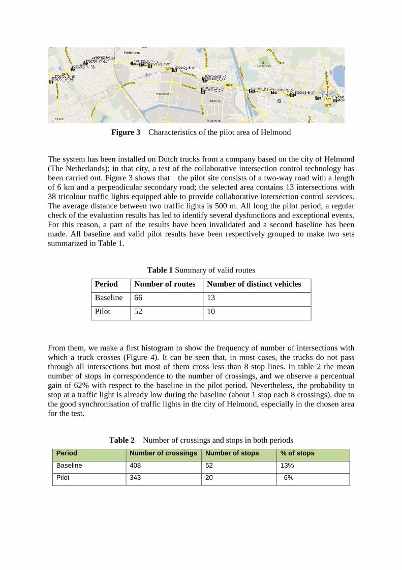
Figure 3 Characteristics of the pilot area of Helmond

The system has been installed on Dutch trucks from a company based on the city of Helmond (The Netherlands); in that city, a test of the collaborative intersection control technology has been carried out. Figure 3 shows that the pilot site consists of a two-way road with a length of 6 km and a perpendicular secondary road; the selected area contains 13 intersections with 38 tricolour traffic lights equipped able to provide collaborative intersection control services. The average distance between two traffic lights is 500 m. All long the pilot period, a regular check of the evaluation results has led to identify several dysfunctions and exceptional events. For this reason, a part of the results have been invalidated and a second baseline has been made. All baseline and valid pilot results have been respectively grouped to make two sets summarized in Table 1.

Table 1 Summary of valid routes

Period Number of routes Number of distinct vehicles

Baseline 66 13

Pilot 52 10

From them, we make a first histogram to show the frequency of number of intersections with which a truck crosses (Figure 4). It can be seen that, in most cases, the trucks do not pass through all intersections but most of them cross less than 8 stop lines. In table 2 the mean number of stops in correspondence to the number of crossings, and we observe a percentual gain of 62% with respect to the baseline in the pilot period. Nevertheless, the probability to stop at a traffic light is already low during the baseline (about 1 stop each 8 crossings), due to the good synchronisation of traffic lights in the city of Helmond, especially in the chosen area for the test.

Table 2 Number of crossings and stops in both periods

Period Number of crossings Number of stops % of stops

Baseline 408 52 13%

Pilot 343 20 6%

Figure 4 Distribution histogram of the number of crossings per route

The temporal distribution during the day presents few changes (except during the morning period, mainly between 5h and 9h) (Figure 5). Indeed, in car traffic peak hours (5h-9h) the number of stops increases considerably. Concerning the percentage of stops per traffic light, it is observed that it decreases during the pilot. Another observation is that the variability is lower during the pilot.

Figure 5 Temporal distributions of crossings, stops and percentage of stops during the day

(baseline in red and pilot in green)

After that we present the main results of aggregated indicators, obtained from instantaneous estimations. We propose two environmental indicators (CO2 and NOx emissions) and two performance indicators (fuel consumption and average speed). Those indicators are unified and calculated for all position points within the influence area of each intersection (100 m before and 60 m after the intersection). Table 3 shows geometric average results for all fires. We observe an average gain of 13% approximately for fuel consumption and emissions, with an average increase of only 2.6 km/h. However, the differences are important from one intersection to the other. For that reason, results are also presented in a disaggregated way by intersection (Table 4). According to those results, the baseline-pilot variations are different and present a strong variability. We observe maximum savings of up to 85% in CO2 emission and fuel consumption and maximum loses up to 56%. Concerning fuel consumption, the interquartile interval is [+0.50%; -26.40%] and that for CO2 emissions [+1.50%; -2670%]. The speed variations are similar, i.e. the interquartile interval is: [-8.10%; +24.30%]. Those results indicate that the main gains are strongly related to the speed, which is not the case in the other pilot carried out in Lyon (for synthesis reasons, the detailed results of the pilot are not presented here but can be found in Blanco et al., 2012). Indeed, in Lyon, a 13% average gain (in fuel consumption and CO2 emission reduction) is obtained with a small speed variation (2%), which shows that in Lyon’s case, it is the acceleration variation that has a strong impact on the overall gains.

Table 3 Gas emissions, fuel consumption and average speeds

Baseline Pilot Rate of change

CO2 emissions (g/km) 644 562 -13%

NOx emissions (g/km) 3.87 3.33 -14%

Fuel consumption (l/100km) 24 21 -13%

Speed (km/h) 35 36 +2.6%

Table 4 Fuel consumption, CO2 Emissions and speed, by intersection.

Baseline Pilot Fuel consumption CO2 emissions Speed

Intersection Nb vehicles

Nb stops

Nb vehicles

Nb stops Baseline Pilot Variation Baseline Pilot Variation Baseline Pilot Variation

5700101_W_1 21 5 21 5 27,6 22,1 -19,9% 746 602 -19,3% 30 35 16,7%

5700102_W_3 19 2 19 2 21,3 19,1 -10,3% 581 542 -6,7% 27 29 7,4%

5700103_E_6 15 1 15 1 27,4 19,5 -28,8% 730 530 -27,4% 41 44 7,3%

5700103_W_5 19 0 19 0 23,8 11,6 -51,3% 653 330 -49,5% 37 34 -8,1%

5700104_E_8 15 0 15 0 23,5 21,2 -9,8% 637 579 -9,1% 40 29 -27,5%

5700104_W_7 20 2 20 2 28,1 27,5 -2,1% 778 765 -1,7% 13 15 15,4%

5700106_W_9 16 1 16 1 32,1 30,5 -5,0% 858 811 -5,5% 37 39 5,4%

5700701_W_14 2 0 2 0 28,4 28 -1,4% 733 744 1,5% 40 49 22,5%

5700702_E_17 11 2 11 2 17,4 15,9 -8,6% 476 433 -9,0% 31 39 25,8%

5700702_W_16 15 2 15 2 15,6 24 53,8% 419 651 55,4% 39 34 -12,8%

5700704_E_18 17 2 17 2 24,5 21,9 -10,6% 661 589 -10,9% 38 38 0,0%

5700704_E_20 11 1 11 1 20,7 20,8 0,5% 563 562 -0,2% 38 34 -10,5%

5700704_W_19 15 1 15 1 22,2 18,5 -16,7% 604 498 -17,5% 31 39 25,8%

5700704_W_21 15 1 15 1 21,9 16 -26,9% 584 435 -25,5% 41 37 -9,8%

5700901_E_23 11 0 11 0 20,7 29,3 41,5% 567 783 38,1% 37 42 13,5%

5700901_W_22 9 1 9 1 23,3 25,1 7,7% 626 669 6,9% 38 49 28,9%

5700902_E_25 14 2 14 2 16,4 14,5 -11,6% 441 392 -11,1% 37 46 24,3%

5700902_W_24 9 0 9 0 19,9 24,7 24,1% 531 664 25,0% 49 47 -4,1%

5700903_E_27 12 2 12 2 36,8 26,8 -27,2% 993 728 -26,7% 34 39 14,7%

5700903_W_26 9 1 9 1 23,5 17,3 -26,4% 629 456 -27,5% 44 35 -20,5%

5700904_E_29 9 2 9 2 25,9 14,1 -45,6% 690 389 -43,6% 41 51 24,4%

5700904_W_28 7 1 7 1 29,3 30,5 4,1% 774 810 4,7% 40 51 27,5%

5700905_E_31 5 0 5 0 10,1 1,6 -84,2% 273 45 -83,5% 59 68 15,3%

5.2. Mobile device

The mobile device method is described in [4]. That precedent work allowed us to implement and test the data collection method. In this subsection we provide the evaluation results of delivery space booking services, which represent a further step with respect to exploratory route results not focused on delivery space booking evaluation [4]. The pilot action was carried out on the city of Bilbao (Spain) with four pilot delivery bays, Licenciado Poza with three parking spots and Pérez Galdós, General Concha, and Santutxu with two parking spots (Figure 6) (for more details about the pilot evaluation, see [18,19]).

Figure 6 The four delivery spaces in Bilbao

From the data collection, 1693 GPS files were loaded and 1601 are considered valid routes. 1248 routes have at least one delivery stop around the studied delivery spaces. 625 of them (Table5) were selected because the truck stops at a delivery space during the possible hours of reservations (between 8h and 13:30h). Figure 7 shows the time distribution of deliveries near the delivery bays. There are big differences between the baseline and the pilot in General Concha and Pérez Galdós. In both cases, the peak of deliveries moves from the late morning (11h/12h) to 8h/9h. In Pérez Galdós, it is observed that the pilot delivery peak corresponds to that of reservations so the changes could be related to the usage of the delivery space booking service.

Table 5 Recorded stops per delivery space

Pilot site Number of baseline stops Number of pilot stops

General Concha 9 46

Pérez Galdós 30 122

Licenciado Poza 31 102

Santutxu 40 208

Table 6 Quartile distances for each site in each period

Delivery spaces Period Q1 Q2 Q3 Q3 - Q1

Pérez Galdós baseline 43 84 104 61

Pérez Galdós pilot 59 86 131 72

Santutxu baseline 37 74 100 63

Santutxu pilot 68 86 105 37

General Concha baseline 22 57 88 66

General Concha pilot 56 89 119 64

Licenciado Poza baseline 23 49 82 59

Licenciado Poza pilot 22 62 120 99

Figure 7 Hours of deliveries (baseline in red and pilot in green)

7 8 9 10 11 12 13 14

0

20

40

60

80

100

hours

%

GENERAL CONCHA

7 8 9 10 11 12 13 14

0

20

40

60

80

100

hours

%

LICENCIADO POZA

7 8 9 10 11 12 13 14

0

20

40

60

80

100

hours

%

PEREZ GALDÓS

7 8 9 10 11 12 13 14

0

20

40

60

80

100

hours

%

SANTUTXU

The delivery space is located at 70m from the limits of the influence area. If the distance is above 140m, it is considered that the driver makes a move to be well-parked (a U-turn or a bypass). In the baseline period the driver choose easily free spaces along the road and during the pilot period he uses the reserved slots for the DSB system. Moreover, during the baseline period there are very few situations when the driver must be a manoeuvre to be well-parked. However, some of these situations exist during the pilot period due certainly to a extraordinary traffic. The considered distances in Figure 8 are the length between the first point into the influence area and the first point of the delivery stop between 8h and 13:30h. The distribution of the distance travelled to park presents some differences between baseline and pilot and more precisely each delivery bay has a specific behaviour. From now on, General Concha data set is not considered in the analysis because the number of counting is not significant.

0 100 200 300 400 500

0.00

00.

004

0.00

8

LICENCIADO POZA

median distance : baseline = 49 m pilot = 62 mlength (m)

Den

sity

0 100 200 300 400 500

0.00

00.

004

0.00

8

PEREZ GALDÓS

median distance : baseline = 84 m pilot = 86 mlength (m)

Den

sity

0 100 200 300 400 500

0.00

00.

006

SANTUTXU

median distance : baseline = 74 m pilot = 86 mlength (m)

Den

sity

0 100 200 300 400 500

0.00

00.

004

0.00

8

GENERAL CONCHA

median distance : baseline = 57 m pilot = 89 mlength (m)

Den

sity

Figure 8 Distribution of the distances before parking (baseline in red and pilot in green)

Table 6 reports for each DSB and period the quartiles Q1, Q2 and Q3 as well as the inter-quartile distance (Q3-Q1). It is observed that the median (Q2) is slightly higher in the pilot period than in the baseline period for all the pilot sites and only for Santutxu the interquartile distance (Q3-Q1) decreases. Erreur ! Source du renvoi introuvable.Table 7 shows that in Licenciado Poza and Pérez Galdos the average of distances during the baseline period is lower than the one of the pilot period (that are upper 140m) but only Pérez Galdós has a p-value with a positive significance. In Santutxu the average of distances is higher in the baseline with a positive significance possibly because the system added a new delivery space, keeping the existing one for deliveries not using the system, but increasing the delivery parking capacity. This is the only transformation of an existing delivery bay into a DSB system. Finally, aggregated evaluation results can be obtained. We report only the results observed in the Santutxu delivery area. First, we show in table 8 the direct gains for a truck on the influence area of each delivery bay, then what it will represent on an average route (which characteristics are defined in [4]).

Table 7 Main distance variations for each site

Site Count Baseline Pilot pvalue significance

General Concha 88 173.9 115.3 0.101

Licenciado Poza 771 112.5 143.3 0.105

Perez Galdós 153 97.9 176.3 0.036 *

Santutxu 427 142.4 108.0 0.015 *

Travel time is intended on the delivery bay’s influence area (the loss is due to the security and the tranquillity drivers feel when legally parking their vehicle with respect to double line parking and other practices). However, another impact of delivery space booking services, less easy to quantify (at least directly from evaluation results) is that of traffic improvement due to the usage of a coherent network of delivery bays. That effect will need to be further quantified, from evaluation data and a simulation with a network of delivery space booking services in a given city, using traffic data and delivery travel behaviour information.

Table 8 Gains on a single DSB (on a 120 m area, Gonzalez-Feliu et al., 2012)

Indicator Without DSB

With DSB

Gap in Freilot areas

Gap in the entire route

Travel distance (m) 147 108 -27% -0.00%

Travel and stop time(min) 15.25 16.92 +11% +0.60%

Fuel consumption (g) 101.4 71.5 -29% -0.08%

CO2 emissions (g) 336 235 -30% -0.01%

NOx emissions (g) 4.1 2.7 -34% -0.01%

6. Conclusion

In this chapter we proposed an overview of GPS-based data collection methods for urban goods movement identification and characterization. Although his field is starting to be explored in the context of urban goods movement, we observe that both fixed and mobile devices can be used to obtain basic information about vehicle position, speed and acceleration in almost instantaneous times. We proposed two applications for logistics and environmental evaluation. Five indicators (travel distances, travel times, fuel consumption and two gas emissions) were proposed to respectively show the logistics and environmental performance of two technologies (an intersection control system and a delivery space booking system).

Using a Smartphone gives the advantage that, once the application is ready, it can be installed into any (or almost) mobile phone allowing it, reducing sensibly the cost. Since “all in one” mobile phone tariffs are available and deployed today, this solution gives the possibility to collect a large amount of data with contained costs. Fixed devices are expensive when used only for GPS collection, but since many in-vehicle systems have already a GPS device, collecting data from them remains possible with a higher cost than that of Smartphones but lower than having specific devices. Remains in this case to solve the question of data transfer, but blue tooth technologies are able to transfer the information into the driver’s mobile phone or another data storage tool. However, it is still needed to standardize the data collection procedures and the transferred files, to develop unified data processing tools. In conclusion, GPS data collection is a challenging field in urban goods movement and can give important information with a lower cost, but needs still to be developed in order to reach a maturity status in terms of commercialization and ergonomics.

Acknowledgement

Part of this research has been carried out related to the FREILOT Project (Urban Freight Energy Efficient Pilot), partially financed by the European Commission (ICT Policy Support Program). The authors should also like to thank Rosa Blanco and Marta Miranda from CTAG for their suggestions and comments concerning the computational analyses made during the evaluation, as well as Christian Ambrosini and Jean-Louis Routhier from Université Lyon 2 and Laboratoire d’Economie des Transports for their help concerning the characterisation of urban routes and the urban goods movement background.

References

[1] Ambrosini C, Routhier J L. Objectives, Methods and Results of Surveys Carried out in the Field of Urban Freight Transport: An International Comparison. Transport Reviews 2004; 24 (1):57–77.

[2] Allen J and Browne M. Review of Survey Techniques Used in Urban Freight Studies. Research Report. University of Westminster, UK, 2008.

[3] Allen J, Browne M, Cherrett T, et al. Survey Techniques in Urban Freight Transport Studies, Transport Reviews 2012; 32(3):287-311.

[4] Pluvinet P, Gonzalez-Feliu J, Ambrosini C, et al. GPS data analysis for understanding urban goods movement. Procedia Social and Behavioral Science 2012; 39:450-462.

[5] Greaves S P, Figliozzi M A. Collecting Commercial Vehicle Tour Data with Passive Global Positioning System Technology. Issues and Potential Applications. Transportation Research Record 2008; 2049:158–166.

[6] McCabe S, Roorda M, Kwan H, et al. Comparing GPS and Non-GPS Survey Methods for Collecting Urban Goods and Service Movements. In Proceedings of the 8th

International Conference on Survey Methods in Transport: Harmonisation and Data Comparability, Annecy, France, 2008.

[7] Sharman BW, Roorda J. Analysis of Freight Global Positioning System Data. Clustering Approach for Identifying Trip Destinations. Transportation Research Record 2011; 2246:83-91.

[8] Joubert J W, Axhausen K W. Inferring commercial vehicle activities in Gauteng, South Africa. Journal of Transport Geography, doi: 10.1016/j.jtrangeo.2009;10.

[9] Joubert, J.W. A provincial comparison of commercial vehicle movement. Proceedings of the 29th Southern African Transport Conference, Pretoria, South Africa, 2010.

[10] Joubert J W. Analyzing commercial through-traffic. Procedia Social and Behavioral Sciences 2012; 39:184-194.

[11] Comendador J, Lopez-Lamba M E, Monzon A. GPS analysis for urban freight distribution, Procedia Social and Behavioral Science 2012; 39:521-533.

[12] Yokota T and Tamagawa D. An Analysis of Urban Freight Transport Behaviour Using A Probe Car System-A Case Study of Keihanshin Area in Japan. WCTR Proceedings Lisbon, 2010: 1-22.

[13] Yokota T and Tamagawa D. Constructing Two-layered Freight Traffic Network Model from Truck Probe Data. International Journal of Intelligent Transportation Systems Research 2011;9(1):1-11.

[14] Yokota T and Tamagawa D. Route Identification of Freight Vehicle's Tour Using GPS Probe Data and its Application to Evaluation of on and off Ramp Usage of Expressways, Procedia Social and Behavioral Science 2012; 39: 255-266.

[15] Holguin-Veras J and Patil G R. Observed trip chain behavior of commercial vehicles, Transportation Research Record 2005; 1906: 74-80.

[16] Patier D, Routhier J L. Une méthode d’enquête du transport de marchandises en ville pour un diagnostic en politiques urbaines. Les Cahiers Scientifiques du Transport 2009; 55:11-38.

[17] Routhier J L, Traisnel J P, Gonzalez-Feliu J, Henriot F, Raux C, et al. ETHEL II: Energie, Transport, Habitat, Environment, Localisations. GICC-ADEME, France, 2009.

[18] Blanco R, Garcia E, Novo I, Tevell M, Thebaud, J B, Thurksma S, Koenders E, Uriarte A, Gonzalez-Feliu J, Pluvinet P, Zubillaga F, Salanova J M. FREILOT – Urban Freight Energy Efficiency Pilot. Evaluation methodology and plan. Ertico-ITS, Brussels, 2010.

[19] Blanco R, Garcia E, Rodriguez R, Novo I, Sartre V, Turksma S, Koenders E, Uriarte A, Gonzalez-Feliu J, Pluvinet P, Zubillaga Elorza F, Salanova J M. FREILOT – Urban Freight Energy Efficiency Pilot. Evaluation results. Ertico–ITS, Brussels, 2012.

[20] Ademe. Logiciel Impact-Ademe. Emissions de polluants et consommation liées à la circulation routière. Ademe Editions, Angers, France, 2003.

[21] André, M. (2004), The ARTEMIS European driving cycles for measuring car pollutant emissions, Science of the total environment, Vol. 334–335, pp. 73-84.

[22] Barth M, Scora G, Younglove T, et al. Modal emissions model for heavy-duty diesel vehicles. Transportation Research Record 2004; 1880:10-20.

[23] Barth M, An F, Norbeck J, Ross M, et al. Modal emissions modelling: a physical approach. Transportation Research Record 1996; 1520:81-88

[24] Bonnafous A. Le siècle des ténèbres de l’économie. Economica, Paris, 1989.

[25] Gonzalez-Feliu J, Faivre d’Arcier B, Rojas N, Basck P, Gardrat M, Vernoux G, Lekuona G, Zubillaga F. FREILOT – Urban Freight Energy Efficiency Pilot. D.FL.6.4. Cost-benefit analysis. Ertico – ITS, Brussels, 2012.