gps occultation introduction and overvie 16, 2009 atmo/opti 656b kursinski et al. 1 gps occultation...

April 16, 2009 ATMO/OPTI 656b Kursinski et al. 1

GPS Occultation IntroductionGPS Occultation Introductionand Overviewand Overview

R. Kursinski

Dept. of Atmospheric Sciences, University of Arizona, Tucson AZ, USA


Occultation GeometryOccultation Geometry

An occultation occurs whenAn occultation occurs whenthe orbital motion of a GPSthe orbital motion of a GPSSV and a Low Earth OrbiterSV and a Low Earth Orbiter(LEO) are such that the LEO(LEO) are such that the LEO‘‘seessees’’ the GPS rise or set the GPS rise or setacross the limbacross the limb

This causes the signal pathThis causes the signal pathbetween the GPS and the LEObetween the GPS and the LEOto slice through the atmosphereto slice through the atmosphere

α

Occultation geometry

The basic observable is the change in the delay of the signal pathThe basic observable is the change in the delay of the signal pathbetween the GPS SV and LEO during the occultationbetween the GPS SV and LEO during the occultation

The change in the delay includes the effect of the atmosphere which actsThe change in the delay includes the effect of the atmosphere which actsas a planetary scale lens bending the signal pathas a planetary scale lens bending the signal path


GPS Occultation CoverageGPS Occultation CoverageTwo Two occultations occultations per orbit per LEO-GPS pairper orbit per LEO-GPS pair =>14 LEO orbits per day and 24 GPS SV =>14 LEO orbits per day and 24 GPS SV

=>=>Occultations Occultations per day ~ 2 x 14 x 24 ~700per day ~ 2 x 14 x 24 ~700 =>500 =>500 occultations occultations within within ++4545oo of velocity vector per day of velocity vector per day

per orbiting GPS receiver distributedper orbiting GPS receiver distributed globallyglobally

DistributionDistributionof one day ofof one day ofoccultationsoccultations


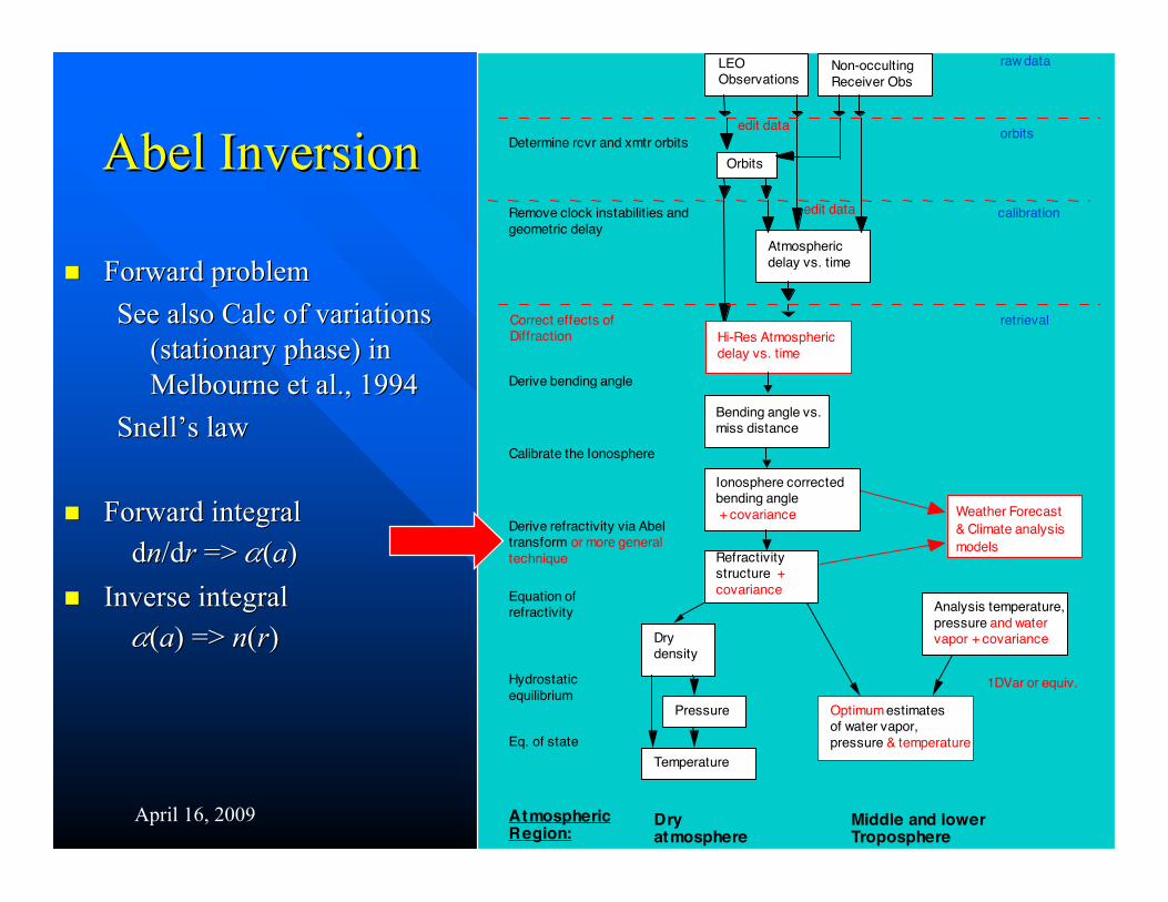
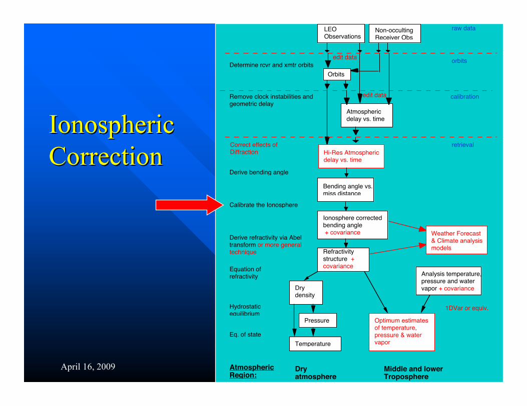
OverviewOverviewDiagram ofDiagram ofProcessingProcessing

Figure shows steps inFigure shows steps inthe processing ofthe processing ofoccultation dataoccultation data

Remove clock instabilities and geometric delay

Refractivity structure + covariance

Drydensity

Pressure

Temperature

Optimum estimates of temperature, pressure & water vapor

Hydrostaticequilibrium

Eq. of state

Equation of refractivity Analysis temperature,

pressure and water vapor + covariance

Middle and lower Troposphere

Dry atmosphere

Atmospheric Region:

LEO Observations

Non-occulting Receiver Obs

Orbits

Bending angle vs.miss distance

Ionosphere corrected bending angle + covariance

Calibrate the Ionosphere

Atmospheric delay vs. time

Derive bending angle

Determine rcvr and xmtr orbits

Derive refractivity via Abeltransform or more general technique

Hi-Res Atmospheric delay vs. time

Correct effects ofDiffraction

1DVar or equiv.

Weather Forecast & Climate analysis models

raw data

orbits

calibration

retrieval

edit data

edit data


Talk Outline:Talk Outline: Overview of main steps in processing RO signals.Overview of main steps in processing RO signals.

Occultation GeometryOccultation Geometry

Abel transform pairAbel transform pair

Calculation of the bending angles from Doppler.Calculation of the bending angles from Doppler.

Conversion to atmospheric variables (Conversion to atmospheric variables (rr , P, T, q), P, T, q)

Vertical and horizontal resolution of ROVertical and horizontal resolution of RO

Outline of the main difficulties of RO soundingsOutline of the main difficulties of RO soundings(residual (residual ionospheric ionospheric noise, upper boundarynoise, upper boundaryconditions, conditions, multipathmultipath, super-refraction), super-refraction)


Abel InversionAbel InversionRemove clock instabilities and geometric delay


Dry density

Pressure

Temperature

Optimum estimates of water vapor, pressure & temperature

Hydrostatic equilibrium

Eq. of state




Dry atmosphere

Atmospheric Region:

LEO Observations


Orbits

Bending angle vs. miss distance






Derive refractivity via Abel transform or more general technique


Correct effects of Diffraction

1DVar or equiv.


raw data

orbits

calibration

retrieval

edit data

edit data

Forward problemForward problemSee also Calc of variationsSee also Calc of variations

(stationary phase) in(stationary phase) inMelbourne et al., 1994Melbourne et al., 1994

SnellSnell’’s laws law

Forward integralForward integral ddnn/d/drr => => ((aa))

Inverse integralInverse integral ((aa) => ) => nn((rr))


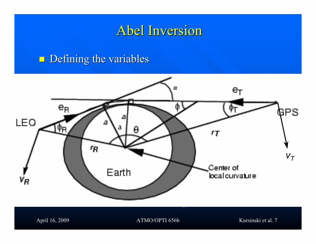
Abel InversionAbel Inversion

Defining the variablesDefining the variables

vT

a


The Bending EffectThe Bending Effect The differential equation for The differential equation for raypaths raypaths can be derived [can be derived [Born and WolfBorn and Wolf, 1980], 1980]

asas (1)(1)

where is poswhere is posiition along the tion along the raypath raypath and and dsds is an incremental length along theis an incremental length along theraypath raypath such thatsuch that (2)(2)

where is the unit vector in the direction along the where is the unit vector in the direction along the raypathraypath.. Consider the change in the quantity, Consider the change in the quantity, , , along the along the raypath raypath given asgiven as

(3)(3) From (2), the first term on the right is zero and from (1), (3) becomesFrom (2), the first term on the right is zero and from (1), (3) becomes

(4)(4) (4) shows that only the (4) shows that only the non-radialnon-radial portion of the gradient of index of portion of the gradient of index of

refraction contributes to changes in .refraction contributes to changes in . So for a spherically symmetric atmosphere, So for a spherically symmetric atmosphere, aa = = nn rr sin sinφφ = constant= constant (5)(5)

((BouguerBouguer’’s s rule )rule )

nds

rdn

ds

d!="

#

$%&

'r

dssrd ˆ=r

rr

s

snr ˆ!r

( ) ( )snds

drsn

ds

rdsnr

ds

dˆˆˆ !+!=!

rr

r

( ) nds

drsnr

ds

d!"="

rrˆ

snr ˆ!r


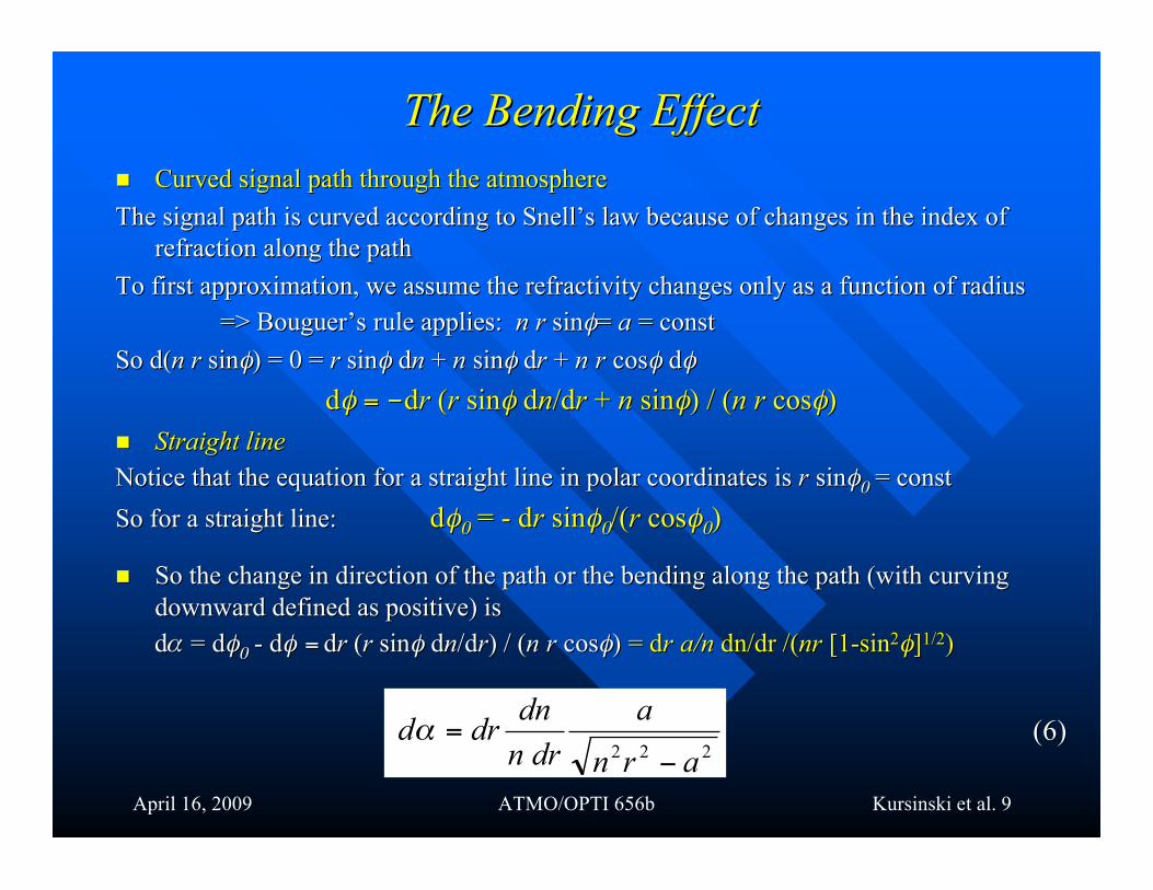
The Bending EffectThe Bending Effect Curved signal path through the atmosphereCurved signal path through the atmosphereThe signal path is curved according to SnellThe signal path is curved according to Snell’’s law because of changes in the index ofs law because of changes in the index of

refraction along the pathrefraction along the pathTo first approximation, we assume the refractivity changes only as a function of radiusTo first approximation, we assume the refractivity changes only as a function of radius

=> => BouguerBouguer’’s s rule applies: rule applies: n r n r sinsinφφ= = aa = const = constSo d(So d(n r n r sinsinφφ) = 0 = ) = 0 = rr sin sinφφ d dnn + + nn sin sinφφ d drr + + nn rr coscosφφ ddφφ

ddφφ = = --ddrr ((rr sin sinφφ d dnn/d/drr + + nn sin sinφφ) / () / (nn rr coscosφφ)) Straight lineStraight lineNotice that the equation for a straight line in polar coordinates is Notice that the equation for a straight line in polar coordinates is rr sin sinφφ00 = const = constSo for a straight line: So for a straight line: ddφφ00 = - = - ddrr sinsinφφ00/(/(rr cos cosφφ00))

So the change in direction of the path or the bending along the path (with curvingSo the change in direction of the path or the bending along the path (with curvingdownward defined as positive) isdownward defined as positive) isdd = d= dφφ00 - d - dφφ == ddrr ((rr sin sinφφ d dnn/d/drr) / () / (nn rr coscosφφ)) = = ddrr a/na/n dn/dr dn/dr /(/(nrnr [1-sin [1-sin22φφ]]1/21/2))

222arn

a

drn

dndrd

!=" (6)(6)


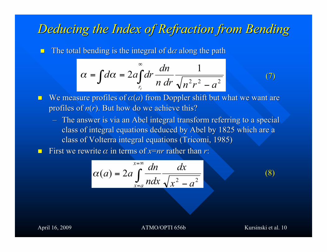
Deducing the Index of Refraction from BendingDeducing the Index of Refraction from Bending The total bending is the integral of The total bending is the integral of dd along the pathalong the path

!!"

#==

trarndrn

dndrad

222

12$$

We measure profiles of We measure profiles of ((aa)) from Doppler shift but what we want are from Doppler shift but what we want areprofiles of profiles of nn((rr). But how do we achieve this?). But how do we achieve this?–– The answer is via an Abel integral transform referring to a specialThe answer is via an Abel integral transform referring to a special

class of integral equations deduced by Abel by 1825 which are aclass of integral equations deduced by Abel by 1825 which are aclass of class of Volterra Volterra integral equations (integral equations (TricomiTricomi, 1985), 1985)

First we rewrite First we rewrite in terms of in terms of xx==nrnr rather than rather than rr::

222)(

ax

dx

ndx

dnaa

x

ax != "

#=

=

$ (8)(8)

(7)(7)


Deducing the Index of Refraction from BendingDeducing the Index of Refraction from Bending We multiply each side of (8) by the kernel, (We multiply each side of (8) by the kernel, (aa22--aa11

22))-1/2-1/2, and integrate with, and integrate withrespect to respect to aa from from aa11 to infinity ( to infinity (Fjeldbo Fjeldbo et al, 1971).et al, 1971).

! !!"=

=

"=

=

"

#$

%&'

(

))=

)

a

aa

x

axa

da

ax

dx

ndx

dn

aa

a

aa

daa

11

222

1

22

1

2

2)(*

dxax

aa

ndx

dn

xa

aa

x

ax

=

=

!"=

= ##$

%

&&'

(

!

!= )

11

2

1

2

2

1

2

1sin2

( )[ ]01

ln

1

rndxndx

dnx

ax

!! "== #$=

=

dx

axaa

daa

ndx

dnxa

aa

x

ax !!

"

#

$$

%

&

''= ((

=

=

)=

=11

222

1

2

2

( )!!

"

#

$$

%

&

''= (

)

1

2

1

201

)(1exp

a aa

daarn

*

+Such thatSuch that

Note thatNote that rr0101 = = aa11//nn((aa11))

(9)(9)


DerivingDerivingBendingBendingfrom Dopplerfrom Doppler



Drydensity

Pressure

Temperature



Eq. of state




Dry atmosphere

Atmospheric Region:

LEO Observations


Orbits










1DVar or equiv.


raw data

orbits

calibration

retrieval

edit data

edit data


Deriving Bending Angles from DopplerDeriving Bending Angles from DopplerThe projection of satellite orbital motion along signal ray-path produces a DopplerThe projection of satellite orbital motion along signal ray-path produces a Doppler

shift at both the transmitter and the receivershift at both the transmitter and the receiverAfter correction for relativistic effects, the Doppler shift, After correction for relativistic effects, the Doppler shift, ffdd, of the transmitter, of the transmitter

frequency, frequency, ffTT, is given as, is given as

vT

( )RRTTT

d eVeVc

ff ˆˆ •+•= ( )RRR

r

RTTT

r

TT VVVVc

f!!!! ""

sincossincos #++#=

where: where: cc is the speed of light and the other variables are defined in the figure with is the speed of light and the other variables are defined in the figure withVVTT

rr andand VVTT representing the radial and representing the radial and azimuthal azimuthal components of thecomponents of the

transmitting spacecraft velocity.transmitting spacecraft velocity.

a

(10)


Deriving Bending Angles from DopplerDeriving Bending Angles from Doppler Solve for aSolve for a Under spherical symmetry, Snell's law => Under spherical symmetry, Snell's law => BouguerBouguer’’s s rule (rule (Born & WolBorn & Wolf, 1980).f, 1980).

n r n r sin sin = constant = = constant = aa = = n n rrtt

where where rrtt is the radius at the tangent point along the ray path.is the radius at the tangent point along the ray path.

So So rrTT sin sin TT = = rrRR sin sin RR = = aa (11)(11)

Given knowledge of the orbital geometry and the center of curvature, we solve Given knowledge of the orbital geometry and the center of curvature, we solvenonlinear equations (10) and (11) iteratively to obtain nonlinear equations (10) and (11) iteratively to obtain TT and and RR andand a a

Solve forSolve for From the geometry of the Figure,From the geometry of the Figure, 2 2 = = TT + + RR + + + + - -

SoSo = = TT + + RR + + –– (12)(12)

Knowing the geometry which provides Knowing the geometry which provides , the angle between the transmitter , the angle between the transmitterand the receiver position vectors, we combine and the receiver position vectors, we combine TT and and R R in (12) to solve for in (12) to solve for ..


Linearized Linearized Relation Between Relation Between , , aa and and ffdd Consider the difference between bent and straight line paths to isolateConsider the difference between bent and straight line paths to isolate

and gain a better understanding of the atmospheric effectand gain a better understanding of the atmospheric effect

vT

aT0

T

The Doppler equation for the straight line path isThe Doppler equation for the straight line path is

( )00000

sincossincos RRR

r

RTTT

r

TT

d VVVVc

ff !!!! "" #++#=

Straight line path

(13)


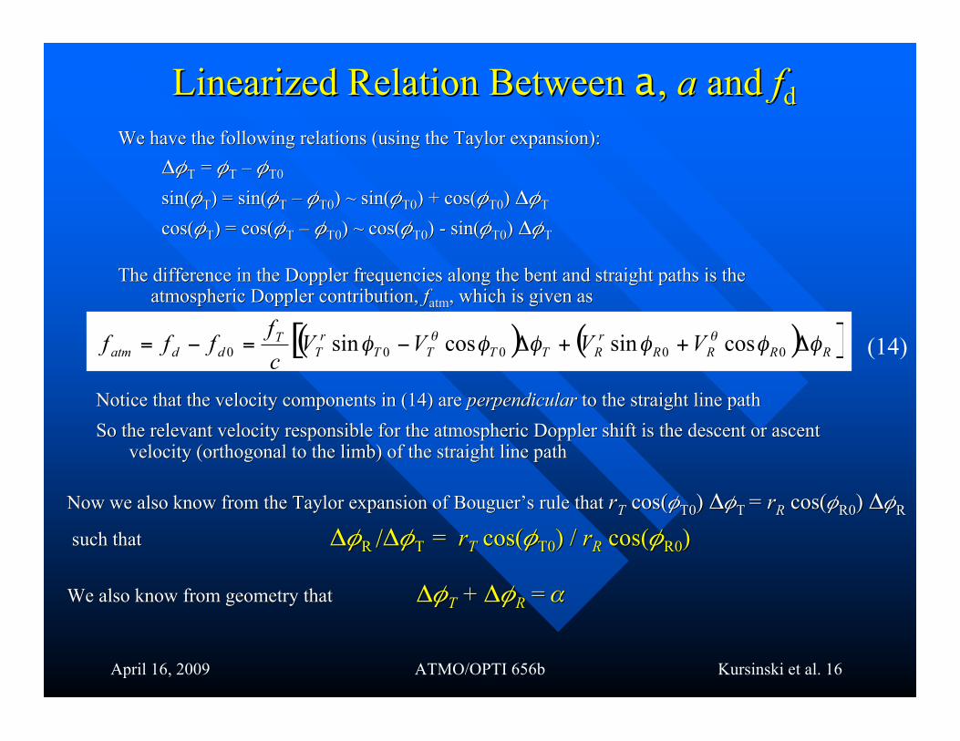
We have the following relations (using the Taylor expansion):We have the following relations (using the Taylor expansion):TT = = TT –– T0T0

sin(sin(TT) = sin() = sin(TT –– T0T0) ~ sin() ~ sin(T0T0) + cos() + cos(T0T0) ) TT

coscos((TT) = ) = coscos((TT –– T0T0) ~ cos() ~ cos(T0T0) - sin() - sin(T0T0) ) TT

The difference in the Doppler frequencies along the bent and straight paths is theThe difference in the Doppler frequencies along the bent and straight paths is theatmospheric Doppler contribution, atmospheric Doppler contribution, ffatmatm, which is given as, which is given as

Linearized Linearized Relation Between Relation Between aa , , aa and and ffdd

( ) ( )[ ]RRRR

r

RTTTT

r

TT

ddatm VVVVc

ffff !!!!!! "" #++#$=$=

00000cossincossin

Notice that the velocity components in (14) are Notice that the velocity components in (14) are perpendicularperpendicular to the straight line path to the straight line pathSo the relevant velocity responsible for the atmospheric Doppler shift is the descent or ascentSo the relevant velocity responsible for the atmospheric Doppler shift is the descent or ascent

velocity (orthogonal to the limb) of the straight line pathvelocity (orthogonal to the limb) of the straight line path

(14)

Now we also know from the Taylor expansion ofNow we also know from the Taylor expansion of Bouguer Bouguer’’s s rule that rule that rrTT cos cos((T0T0)) T T == rrRR cos cos((R0R0)) RR

such thatsuch that R R //T T = = rrTT cos cos((T0T0) /) / rrRR cos cos((R0R0))

We also know from geometry that We also know from geometry that TT ++ RR = =


Now we also know from the Taylor expansion of Now we also know from the Taylor expansion of BouguerBouguer’’s s rule thatrule thatrrTT cos(cos(T0T0) ) T T = = rrRR cos(cos(R0R0) ) RR such thatsuch that

R R //T T = = rrTT cos(cos(T0T0) / ) / rrRR cos(cos(R0R0))

We also know from geometry that We also know from geometry that TT + + RR = =

For the GPS-LEO occultation geometry For the GPS-LEO occultation geometry rrTT cos(cos(T0T0) / ) / rrRR cos(cos(R0R0) ~ 9) ~ 9Therefore Therefore R R //T T ~ 9 ~ 9 and and 1.1 1.1 RR ~ ~ or or RR ~ ~

Therefore we can writeTherefore we can write

So atmospheric Doppler is ~ linearly proportional toSo atmospheric Doppler is ~ linearly proportional to–– bending angle and the straight line descent velocity (typically 2 to 3 km/sec).bending angle and the straight line descent velocity (typically 2 to 3 km/sec).–– 11oo ~ 250 Hz at GPS freq. ~ 250 Hz at GPS freq.

aa ~ ~ rrRR sin(sin(R0R0) + ) + rrRR cos(cos(R0R0) )

Linearized Linearized Relation Between Relation Between , , aa and and ffdd

!"# Vc

ff Tatm

T

atmRRRR

fV

fcrra

!

+"00

cossin ##

Distance fromcenter to straightline tangent point

Distance fromLEO to limb

(15)(15)

(16)(16)


Results from July 1995 from Hajj et al. 2002Results from July 1995 from Hajj et al. 2002 85 GPS/MET 85 GPS/MET occultationsoccultations Note scaling betweenNote scaling between

bending & Doppler residualsbending & Doppler residuals

Angle between transmitter and receiverAngle between transmitter and receiver0 deg. is when tangent height is at 30 km0 deg. is when tangent height is at 30 km

Receiver tracking problemsReceiver tracking problems

ffatmatm ~ ~ ffTT VVperpperp//cc = 1.6x10 = 1.6x1099 x10 x10-5 -5 0.10.1oo*0.017*0.017 rad/rad/oo = 27 Hz= 27 Hz

Bending angles can be larger than 2Bending angles can be larger than 2oo

Implies wet,warm boundary layerImplies wet,warm boundary layer

Straight-

line

Atmo Atmo info contained info contained in small variations in in small variations in


Center of curvatureCenter of curvature The conversion of Doppler to bending angle and asymptotic miss distance depends onThe conversion of Doppler to bending angle and asymptotic miss distance depends on

knowledge of the satellite positions and the reference coordinate center (center ofknowledge of the satellite positions and the reference coordinate center (center ofcurvature)curvature)

The Earth is slightly elliptical such that the center of curvature does not match theThe Earth is slightly elliptical such that the center of curvature does not match thecenter of the Earth in generalcenter of the Earth in general

The center of curvature varies with position on the Earth and the orientation of theThe center of curvature varies with position on the Earth and the orientation of theoccultation planeoccultation plane

The center of curvature is taken asThe center of curvature is taken asthe center of the circle in thethe center of the circle in theoccultation plane that best fits theoccultation plane that best fits thegeoidgeoid near the tangent point near the tangent pointSee Hajj et al. (2002)See Hajj et al. (2002)


Conversion toConversion toAtmosphericAtmospheric

VariablesVariables((rr , P, T, q), P, T, q)



Dry density

Pressure

Temperature



Eq. of state




Dry atmosphere

Atmospheric Region:

LEO Observations


Orbits










1DVar or equiv.


raw data

orbits

calibration

retrieval

edit data

edit data

N equationN equation

Deriving Deriving PP and and TT in indry conditionsdry conditions

Deriving water vaporDeriving water vapor


Conversion to Atmospheric Variables (Conversion to Atmospheric Variables (rr , P, T, q), P, T, q)

Refractivity equation: Refractivity equation: NN = ( = (nn-1)*10-1)*1066 = c = c11 nndd + c+ c22 nnww + c+ c3 3 nnee + c+ c44 nnppnn : index of refraction = c/v : index of refraction = c/v NN : refractivity : refractivitynndd , , nnww , , nnee , , nnpp : number density of : number density of ““drydry”” molecules, water vapor molecules, free molecules, water vapor molecules, free

electrons electrons and particles respectivelyand particles respectively

PolarizabilityPolarizability: : ability of incident electric field to induce an electric dipole ability of incident electric field to induce an electric dipole moment in the molecule (see Atkins 1983, p. 356)moment in the molecule (see Atkins 1983, p. 356)

Dry term: Dry term: a a polarizability polarizability term reflecting the weighted effects of Nterm reflecting the weighted effects of N22, O, O22, A, Aand COand CO22

Wet term:Wet term: Combined Combined polarizability polarizability and permanent dipole terms with and permanent dipole terms with permanent term >> permanent term >> polarizability polarizability term:term:

cc22 nnww = (c= (cw1w1 + c + cw2w2 /T) /T) nnww11stst term is term is polarizabilitypolarizability, 2, 2ndnd term is permanent dipole term is permanent dipole

Ionosphere term:Ionosphere term: Due first order to plasma frequency, proportional to 1/Due first order to plasma frequency, proportional to 1/ff22..Particle term:Particle term: Due to water in liquid and/or ice form. Depends on water amount.Due to water in liquid and/or ice form. Depends on water amount.

No dependence on particle size as long as particles << No dependence on particle size as long as particles << , the GPS, the GPSwavelengthwavelength

(12)(12)


Conversion to atmospheric variables (Conversion to atmospheric variables (rr , P, T, q), P, T, q)

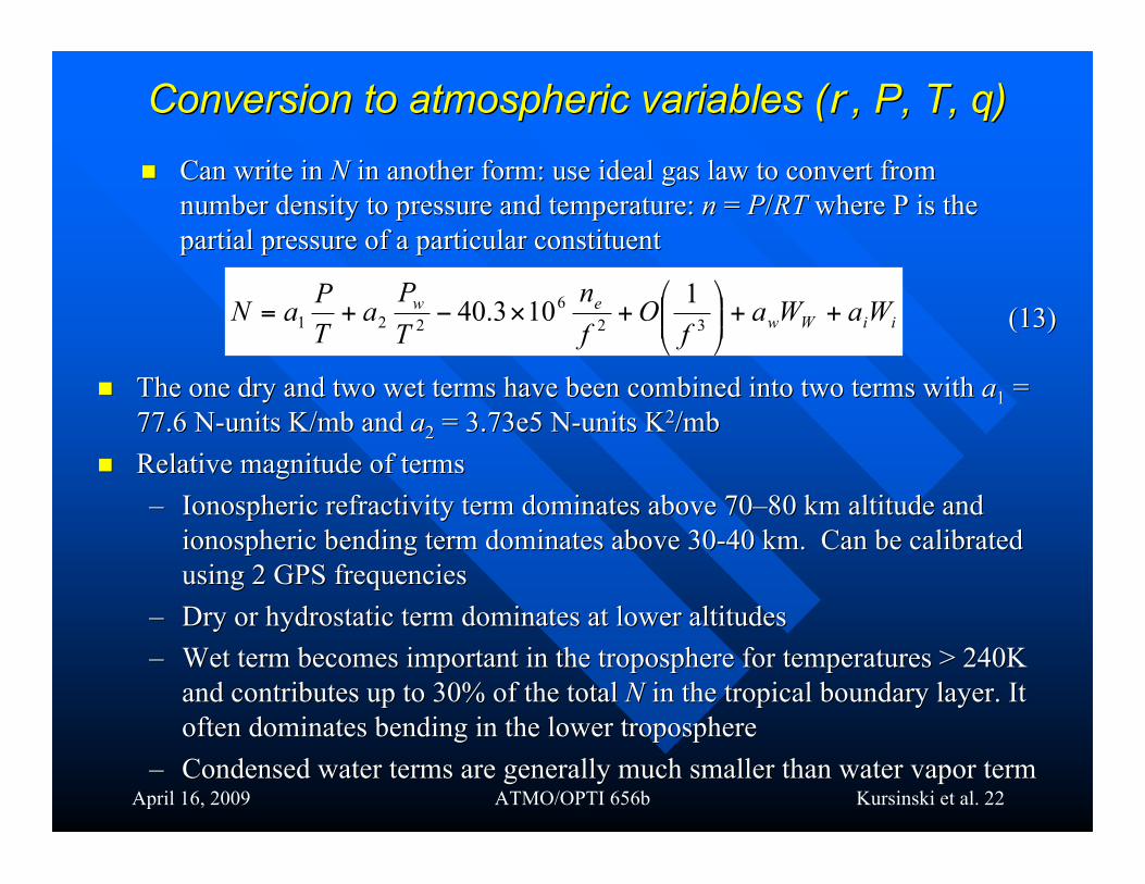
Can write in Can write in NN in another form: use ideal gas law to convert from in another form: use ideal gas law to convert fromnumber density to pressure and temperature: number density to pressure and temperature: nn = = PP//RT RT where P is thewhere P is thepartial pressure of a particular constituentpartial pressure of a particular constituent

The one dry and two wet terms have been combined into two terms with The one dry and two wet terms have been combined into two terms with aa11 = =77.6 N-units 77.6 N-units K/mb K/mb and and aa22 = 3.73e5 N-units K = 3.73e5 N-units K22/mb/mb

Relative magnitude of termsRelative magnitude of terms–– Ionospheric Ionospheric refractivity term dominates above 70refractivity term dominates above 70––80 km altitude and80 km altitude and

ionospheric ionospheric bending term dominates above 30-40 km. Can be calibratedbending term dominates above 30-40 km. Can be calibratedusing 2 GPS frequenciesusing 2 GPS frequencies

–– Dry or hydrostatic term dominates at lower altitudesDry or hydrostatic term dominates at lower altitudes–– Wet term becomes important in the troposphere for temperatures > 240KWet term becomes important in the troposphere for temperatures > 240K

and contributes up to 30% of the total and contributes up to 30% of the total NN in the tropical boundary layer. It in the tropical boundary layer. Itoften dominates bending in the lower troposphereoften dominates bending in the lower troposphere

–– Condensed water terms are generally much smaller than water vapor termCondensed water terms are generally much smaller than water vapor term

iiWwew WaWa

fO

f

n

T

Pa

T

PaN ++!!

"

#$$%

&+'(+=

32

6

221

1103.40 (13)(13)


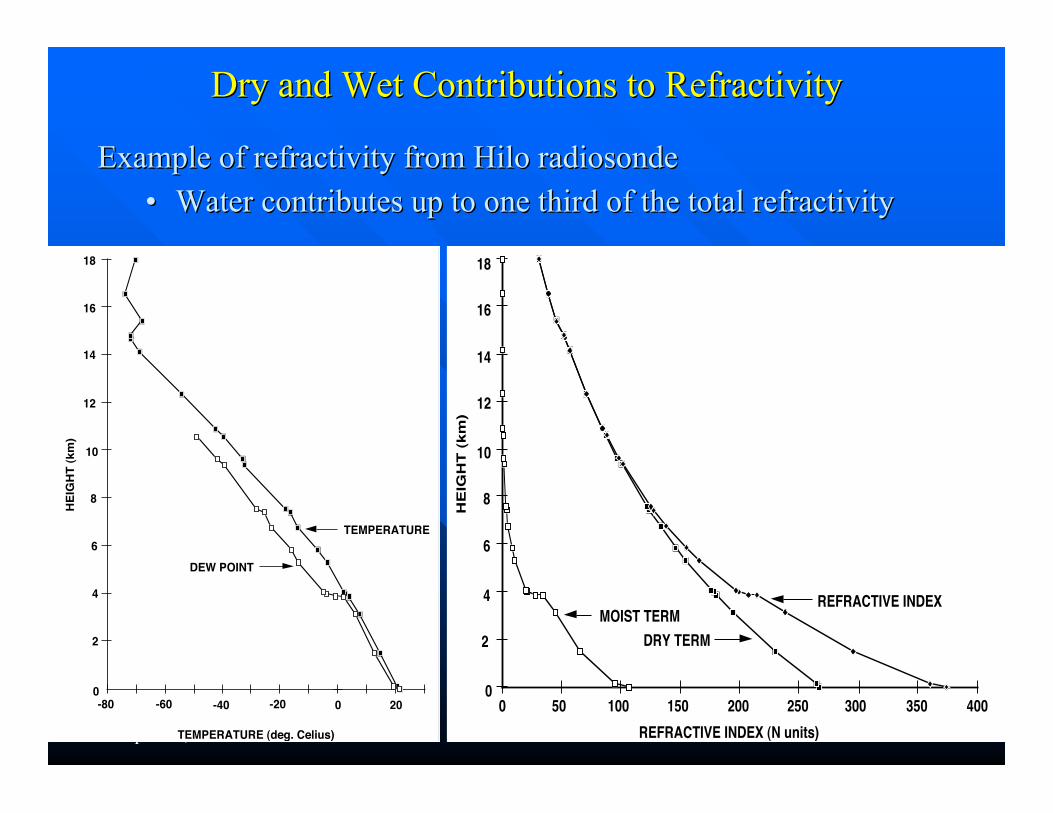
Dry and Wet Contributions to RefractivityDry and Wet Contributions to Refractivity

0 20-20-40-600

2

4

6

8

10

12

14

16

18

TEMPERATURE (deg. Celius)

HE

IGH

T (

km

)

TEMPERATURE

DEW POINT

-80

REFRACTIVE INDEX

0

2

4

6

8

10

12

14

16

18

HE

IGH

T (

km

)

DRY TERM

MOIST TERM

0 50 100 150 200 250 300 350 400

REFRACTIVE INDEX (N units)

Example of refractivity from Hilo Example of refractivity from Hilo radiosonderadiosonde•• Water contributes up to one third of the total refractivityWater contributes up to one third of the total refractivity


Deriving Temperature & PressureDeriving Temperature & Pressure After converting After converting ffdd => => ((aa) => ) => nn((rr) and removing effects of ionosphere, from) and removing effects of ionosphere, from

(12) we have a profile of dry molecule number density for altitudes between(12) we have a profile of dry molecule number density for altitudes between50-60 km down to the 240K level in the troposphere:50-60 km down to the 240K level in the troposphere:

nnd d ((zz) = ) = NN((zz)/c)/c11 = [ = [nn((zz)-1]*10)-1]*106 6 /c/c11 We know the dry constituents are well mixed below ~100 km altitude so We know the dry constituents are well mixed below ~100 km altitude so cc11

and the mean molecular mass, and the mean molecular mass, µµdd, are well known across this interval., are well known across this interval. We apply hydrostatic equation, We apply hydrostatic equation, dP dP = -= -gg rr ddz z = -g = -g nndd µµdd d dzz to derive a verticalto derive a vertical

profile of pressure versus altitude over this altitude interval.profile of pressure versus altitude over this altitude interval.

)()()( top

z

z

ddtop

z

z

zPdzgnzPdzgzP

toptop

+=+= !! µ"

We need an upper boundary condition, We need an upper boundary condition, PP((zztoptop) which must be estimated from) which must be estimated fromclimatologyclimatology, weather analyses or another source, weather analyses or another source

Given Given PP(z) and (z) and nndd(z), we can solve for (z), we can solve for TT((zz) over this altitude interval using) over this altitude interval usingthe equation of state (ideal gas law): the equation of state (ideal gas law): TT((zz) = ) = PP((zz) / () / (nndd((zz) ) RR)) (15)(15)

(14)(14)


GPS Temperature Retrieval ExamplesGPS Temperature Retrieval Examples

GPS lo-res

GPS hi-res

GPS lo-res

GPS hi-res

26

Refractivity ErrorRefractivity Error

Fractional error in refractivity derived by GPS ROFractional error in refractivity derived by GPS RO asasestimated in estimated in Kursinski Kursinski et al. 1997et al. 1997Considers several error sourcesConsiders several error sources

Solar max, low SNR Solar max, low SNR Solar min, high SNRSolar min, high SNR


Error in the height of Pressure surfacesError in the height of Pressure surfaces GPS RO yields pressure versus heightGPS RO yields pressure versus height Dynamics equations are written more compactly withDynamics equations are written more compactly with

pressure as the vertical coordinatepressure as the vertical coordinate where height of awhere height of apressure surface becomes a dependent variablepressure surface becomes a dependent variable

Solar max, low SNR Solar min, high SNRSolar max, low SNR Solar min, high SNR


GPSRO Temperature AccuracyGPSRO Temperature Accuracy

Temperature is proportional to Pressure/DensityTemperature is proportional to Pressure/Density So So TT/T /T = = PP/P /P - - // Very accurate in upper troposphere/lower troposphere (UTLS)Very accurate in upper troposphere/lower troposphere (UTLS)

SolarSolar max, low SNRmax, low SNR Solar min, high SNRSolar min, high SNR


Deriving WaterDeriving WaterVapor from GPSVapor from GPS

OccultationsOccultations Remove clock instabilities and geometric delay


Dry density

Pressure

Temperature



Eq. of state




Dry atmosphere

Atmospheric Region:

LEO Observations


Orbits










1DVar or equiv.


raw data

orbits

calibration

retrieval

edit data

edit data

•• In the middle and lower In the middle and lowertroposphere, troposphere, nn((zz) contains dry and) contains dry andmoist contributionsmoist contributions=>Need additional information=>Need additional information

EitherEither•• Add temperature from an Add temperature from ananalysis to derive water vaporanalysis to derive water vaporprofiles in lower and middleprofiles in lower and middletropospheretroposphere

oror•• Perform Perform variationalvariational assimilation assimilationcombining combining nn((zz) with independent) with independentestimates of estimates of TT, , qq and and PPsurfacesurface and andcovariances covariances of eachof each


Refractivity of Condensed WaterRefractivity of Condensed Water ParticlesParticles

High dielectric constant (~80) of condensed liquid water particlesHigh dielectric constant (~80) of condensed liquid water particlessuspended in the atmosphere slows light propagation via scatteringsuspended in the atmosphere slows light propagation via scattering=>=> Treat particles in air as a dielectric slab Treat particles in air as a dielectric slab

Particles are much smaller than GPS wavelengthsParticles are much smaller than GPS wavelengths=>=> Rayleigh Rayleigh scattering regimescattering regime=>=> Refractivity of particles, Refractivity of particles, NNpp proportional to density of condensedproportional to density of condensed

water in atmosphere, water in atmosphere, WW, and , and independentindependent of particle size of particle sizedistribution.distribution.–– First order discussion given by First order discussion given by KursinskiKursinski [1997].[1997].–– More detailed form of refractivity expression for liquid water given by More detailed form of refractivity expression for liquid water given by LiebeLiebe

[1989].[1989].

Liquid water drops:Liquid water drops: NNpp ~ 1.4 ~ 1.4 WW [where [where WW is in g/m is in g/m33]]Ice crystals:Ice crystals: NNpp ~ 0.6 ~ 0.6 WW [[KursinskiKursinski, 1997]., 1997].Water vapor:Water vapor: NNww ~ 6 ~ 6 rr vv [where [where rr vv is in g/mis in g/m33]]


=>=> Same amount of water in vapor phase creates Same amount of water in vapor phase creates~ 4.4 * refractivity of same amount of liquid water~ 4.4 * refractivity of same amount of liquid water~ 10 * refractivity of same amount of water ice~ 10 * refractivity of same amount of water ice

Liquid water content of clouds is generally less than 10% ofLiquid water content of clouds is generally less than 10% ofwater vapor content (particularly for horizontally extendedwater vapor content (particularly for horizontally extendedclouds)clouds)

=>=> Liquid water refractivity generally less than 2.2% of water Liquid water refractivity generally less than 2.2% of watervapor refractivityvapor refractivity

=>=> Ice clouds generally contribute small fraction of water vapor Ice clouds generally contribute small fraction of water vaporrefractivity at altitudes where water vapor contribution isrefractivity at altitudes where water vapor contribution isalready smallalready small

Clouds will Clouds will veryvery slightly increase apparent water vapor slightly increase apparent water vaporcontentcontent

Refractivity of Condensed Water ParticlesRefractivity of Condensed Water Particles


Deriving Humidity from GPS RODeriving Humidity from GPS RO Two basic approachesTwo basic approaches

‒‒ Direct m ethod : use Direct m ethod : use NN & & TT prof iles and hydrostat ic B.C. prof iles and hydrostat ic B.C.

‒‒ Variat ional Variat ional m ethod : use m ethod : use NN , , TT & & qq prof iles and hydrostat ic B.C. prof iles and hydrostat ic B.C.

w ith error w ith error covariances covariances to update estim ates of to update estim ates of TT , , qq and and PP..

Direct MethodDirect Method

‒‒ Theoretically less accurate than Theoretically less accurate than variat ional variat ional approachapproach

‒‒ Sim ple error m odelSim ple error m odel

‒‒ ( larg ely) insensit ive to NW P model hum id ity errors( larg ely) insensit ive to NW P model hum id ity errors

Variat ional Variat ional MethodMethod

‒‒ Theoretically m ore accurate than sim ple m ethod because ofTheoretically m ore accurate than sim ple m ethod because of

inclusion of inclusion of apriori apriori m oisture inform ationm oisture inform ation

‒‒ Sensit ive to unknown model hum id ity errors and b iasesSensit ive to unknown model hum id ity errors and b iases

Since we are evaluating a m odel we want water vapor estim ates asSince we are evaluating a m odel we want water vapor estim ates as

independent as possib le from modelsindependent as possib le from models

= > W e use the Direct Method= > W e use the Direct Method


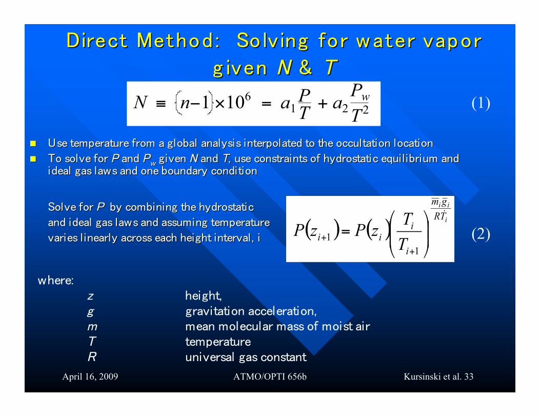
Direct Method : Solving for water vaporDirect Method : Solving for water vapor

g iven g iven NN & & TT

Use temperature from a global analysis interpolated to the occultation locationUse temperature from a global analysis interpolated to the occultation location

To solve for To solve for PP and and PPww given given NN and and TT, use constraints of hydrostatic equilibrium and, use constraints of hydrostatic equilibrium andideal gas laws and one boundary conditionideal gas laws and one boundary condition

where:z height,g gravitation acceleration,m mean molecular mass of moist airT temperatureR universal gas constant

(2)

Solve for Solve for PP by combining the hydrostatic by combining the hydrostatic

and ideal gas laws and assuming temperatureand ideal gas laws and assuming temperature

varies linearly across each height interval, ivaries linearly across each height interval, i ( ) ( )i

ii

TR

gm

i

iiiT

TzPzP

&

!!"

#$$%

&=

+

+

1

1

N ! n"1 #10

6 = a1

P

T+ a2

Pw

T2

(1)


Solving for water vapor given Solving for water vapor given NN & & TTGiven knowledge of Given knowledge of TT((hh) and pressure at some height for a boundary) and pressure at some height for a boundary

condition, then (1) and (2) are solved iteratively as follows:condition, then (1) and (2) are solved iteratively as follows:

1) Assume 1) Assume PPww((hh) = 0 or 50% RH for a first guess) = 0 or 50% RH for a first guess

2) Estimate 2) Estimate PP((hh) via (2)) via (2)

3) Use 3) Use PP((hh) and ) and TT((hh) in (1) to update ) in (1) to update PPww((hh))

4) Repeat steps 2 and 3 until convergence.4) Repeat steps 2 and 3 until convergence.

Standard deviation of fractional Standard deviation of fractional PPww error error ((Kursinski Kursinski et al., 1995):et al., 1995):

where where BB = = aa 11TP TP / / aa 2 2 PPww and and PPss is the surface pressure is the surface pressure

!

"Pw

Pw

= B +1( )2 "

N

2

N2

+ Bs+ 2( )

2 "T

2

T2

+ Bs

2"Ps

2

Ps

2

#

$ %

&

' (

1/ 2


A moisture variable closely related to the GPS observations isA moisture variable closely related to the GPS observations isspecific humidity, specific humidity, qq, the mass mixing ratio of water vapor in, the mass mixing ratio of water vapor inair.air.

Given Given PP and and PPww, , qq, is given by, is given by

q=

md

mw

PPw

!1 +1

!1

Solving for Water Vapor given Solving for Water Vapor given NN & & TT

Note that GPS-derived refractivity is essentially a molecule counterfor “dry” and water vapor molecules.

It is not a direct relative humidity sensor.


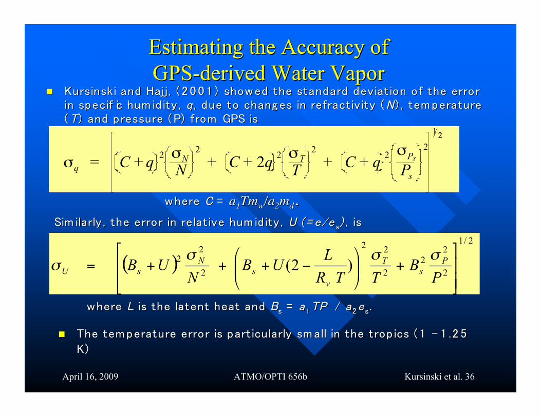
Estimating the Accuracy ofEstimating the Accuracy ofGPS-derived Water VaporGPS-derived Water Vapor

Sim ilarly , the error in relat ive hum id ity , Sim ilarly , the error in relat ive hum id ity , U (U ( = e/e= e/ess)) , is, is

where where LL is the latent heat and is the latent heat and BBss = = aa 11TP TP / / aa 22 ee ss..

The temperature error is part icularly sm all in the trop ics ( 1 - 1 .2 5The temperature error is part icularly sm all in the trop ics ( 1 - 1 .2 5

K)K)

( )

2/1

2

22

2

22

2

22

)2(!!

"

#

$$

%

&+''

(

)**+

,-+++=

PB

TTR

LUB

NUB

P

s

T

v

s

N

sU

....

!q = C + q2 !N

N

2

+ C + 2q2 !T

T

2

+ C + q2 !Ps

Ps

2

12

12

Kursinski Kursinski and Hajj, ( 2 0 0 1 ) showed the standard deviat ion of the errorand Hajj, ( 2 0 0 1 ) showed the standard deviat ion of the errorin specif ic hum id ity , in specif ic hum id ity , qq , due to chang es in refractivity (, due to chang es in refractivity (NN ) , temperature) , temperature(( TT ) and pressure (P) from GPS is) and pressure (P) from GPS is

where where C C = = aa11TmTmww/a/a22mmdd,,


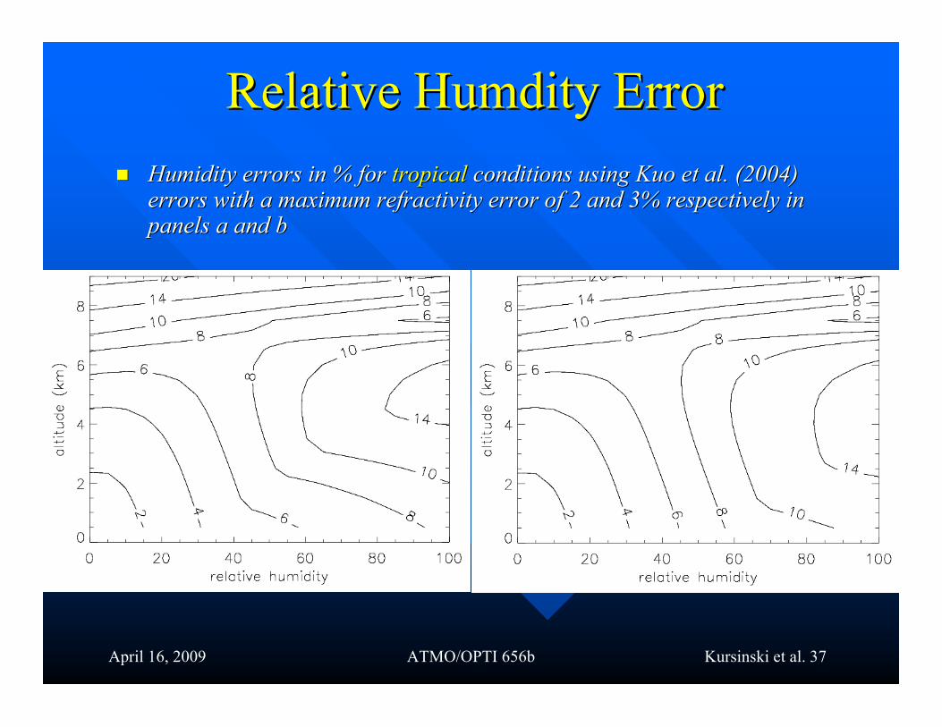
Relative Relative Humdity Humdity ErrorError Humidity errors in % for Humidity errors in % for tropicaltropical conditions using conditions using Kuo Kuo et al. (2004)et al. (2004)

errors with a maximum refractivity error of 2 and 3% respectively inerrors with a maximum refractivity error of 2 and 3% respectively inpanels a and bpanels a and b


Given the GPS observations alone, we have an Given the GPS observations alone, we have an underdeterminedunderdeterminedproblem in solving for problem in solving for PPww

Previously, we assumed knowledge of temperature to provide thePreviously, we assumed knowledge of temperature to provide themissing information & solve this problem.missing information & solve this problem.

However, temperature estimates have errors that we shouldHowever, temperature estimates have errors that we shouldincorporate into our estimateincorporate into our estimate

If we combine If we combine aprioriapriori estimates of temperature estimates of temperature andand water from a water from aforecast or analysis with the GPS refractivity estimates we createforecast or analysis with the GPS refractivity estimates we createan an overdeterminedoverdetermined problemproblem

=> => We can use a least squares approach to find the optimal We can use a least squares approach to find the optimal solutionssolutionsfor for TT, , PPww and and P.P.

Variational Variational Estimation of WaterEstimation of Water


Variational Variational Estimation of WaterEstimation of WaterIn a In a variational variational retrieval, the most probable atmospheric state, retrieval, the most probable atmospheric state, xx, is calculated by, is calculated by

combining combining a prioria priori (or background) atmospheric information, (or background) atmospheric information, xxbb, with, withobservations, observations, yyoo, in a statistically optimal way., in a statistically optimal way.

The solution, The solution, xx, gives the best fit - in a least squared sense - to both the observations, gives the best fit - in a least squared sense - to both the observationsandand a priori a priori information. information.

For Gaussian error distributions, obtaining the most probable state is equivalent toFor Gaussian error distributions, obtaining the most probable state is equivalent tofinding the finding the xx that minimizes a cost function, that minimizes a cost function, J(x),J(x), given by given by

J(x) = 12

x – xb TB

– 1x – xb + 1

2yo – H (x)

TE + F

– 1yo – H (x)

where:• B is the background error covariance matrix.• H(x) is the forward model, mapping the atmospheric information x intomeasurement space.• E and F are the error covariances of measurements and forward model respectively.• Superscripts T and –1 denote matrix transpose and inverse.


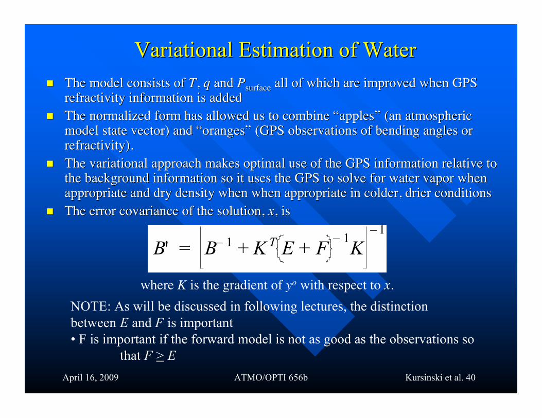
The model consists of The model consists of TT, , qq and and PPsurfacesurface all of which are improved when GPSall of which are improved when GPSrefractivity information is addedrefractivity information is added

The normalized form has allowed us to combine The normalized form has allowed us to combine ““applesapples”” (an atmospheric (an atmosphericmodel state vector) and model state vector) and ““orangesoranges”” (GPS observations of bending angles or (GPS observations of bending angles orrefractivity).refractivity).

The The variational variational approach makes optimal use of the GPS information relative toapproach makes optimal use of the GPS information relative tothe background information so it uses the GPS to solve for water vapor whenthe background information so it uses the GPS to solve for water vapor whenappropriate and dry density when when appropriate in colder, drier conditionsappropriate and dry density when when appropriate in colder, drier conditions

The error covariance of the solution, The error covariance of the solution, xx, is, is

Variational Variational Estimation of WaterEstimation of Water

B' = B

– 1+ K

TE + F

– 1

K

– 1

where K is the gradient of yo with respect to x. NOTE: As will be discussed in following lectures, the distinctionbetween E and F is important• F is important if the forward model is not as good as the observations so

that F > E


Variational Variational Estimation of Water:Estimation of Water:Advantages & DisadvantagesAdvantages & Disadvantages

The solution is theoretically better than the solutionThe solution is theoretically better than the solutionassuming only temperatureassuming only temperature

The solution is limited to the model levels and GPSThe solution is limited to the model levels and GPSgenerally has higher vertical resolution than modelsgenerally has higher vertical resolution than models

The solution is as good as its assumptionsThe solution is as good as its assumptions–– Unbiased Unbiased aprioriapriori–– Correct error Correct error covariancescovariances

Model constraints are significant in defining the Model constraints are significant in defining the aprioriaprioriwater estimates and may therefore yield unwanted modelwater estimates and may therefore yield unwanted modelbiases in the resultsbiases in the results

Temperature approach provides more independentTemperature approach provides more independentestimate of water vaporestimate of water vapor


Vertical and Horizontal Resolution of ROVertical and Horizontal Resolution of RO

Resolution associated with distributedResolution associated with distributedbending along the bending along the raypathraypath

Diffraction limited vertical resolutionDiffraction limited vertical resolution Horizontal resolutionHorizontal resolution


Resolution: Bending Contribution along the Resolution: Bending Contribution along the RaypathRaypath

Contribution to bending estimated from each 250 m verticalContribution to bending estimated from each 250 m verticalintervalinterval

Results based on aResults based on aradiosonderadiosonde profile profilefrom Hilo, Hawaiifrom Hilo, Hawaii

Left panel shows theLeft panel shows thevertical interval oververtical interval overwhich half the bendingwhich half the bendingoccursoccurs

Demonstrates howDemonstrates howfocused thefocused thecontribution is to thecontribution is to thetangent regiontangent region


Fresnel’s Volume: Applicability of Geometric Optics.Generally, EM field at receiver depends on the refractivity in all space.In practice, it depends on the refractivity in the finite volume around thegeometric-optical ray (Fresnel’s volume).The Fresnel’s volume characterizes the physical “thickness” of GO ray.The Fresnel’s volume in a vacuum:

aaff

ll22ll11

2/21

22

2

22

1!=""+++ llalal ff

21

21

ll

lla f

+=

!The Fresnel’s zone (cross-section of the Fresnel’s volume):

Two rays may be considered independent when their Fresnel’s volumesdo not overlap.Geometric optics is applicable when transverse scales of N-irregularitiesare larger than the diameter of the first Fresnel zone.


Atmospheric Effects on the First Atmospheric Effects on the First Fresnel Fresnel Zone DiameterZone Diameter Without bending, 2 Without bending, 2 aaff ~ 1.4 km for a LEO-GPS occultation~ 1.4 km for a LEO-GPS occultation The atmosphere affects the size of the first The atmosphere affects the size of the first Fresnel Fresnel zonezone,, generally making it smaller generally making it smaller The bending gradient, The bending gradient, dd/d/daa, causes defocusing which also causes a more rapid, causes defocusing which also causes a more rapid

increase in length vertically away from the tangent point such that the increase in length vertically away from the tangent point such that the /2 criterion is/2 criterion ismet at a smaller distance than met at a smaller distance than aaff ..

0 0.5 1 1.5

Diameter of first Fresnel zone (km)

0.01 0.1 1

Relative Intensity

0

5

10

15

20

25

30

35

40a b

Altitu

de

(km

)

=> The => The Fresnel Fresnel zone diameter and resolution is estimated from the amplitude datazone diameter and resolution is estimated from the amplitude data

Large defocusingLarge defocusing High resolutionHigh resolution

Large focusingLarge focusing Low resolutionLow resolution


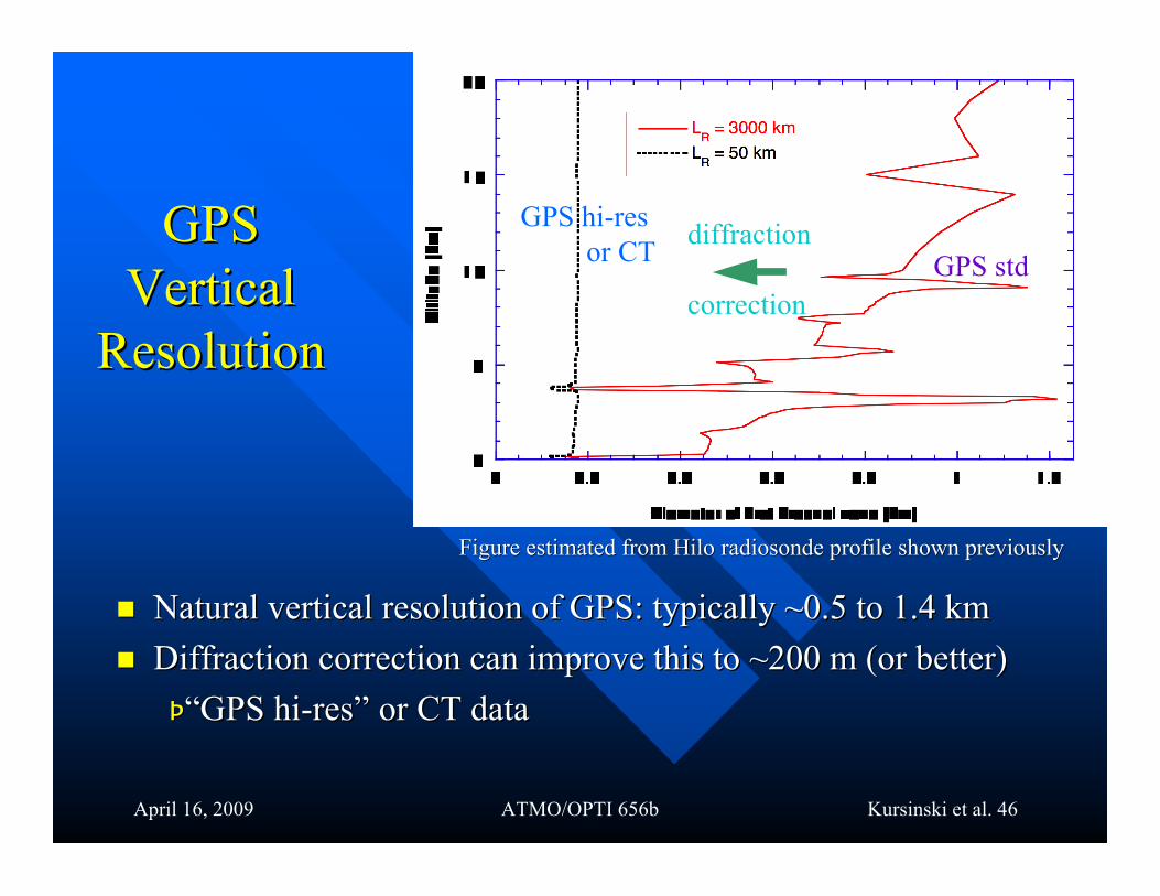
GPSGPSVerticalVertical

ResolutionResolution

GPS std

GPS hi-res or CT

Natural vertical resolution of GPS: typically ~0.5 to 1.4 km Natural vertical resolution of GPS: typically ~0.5 to 1.4 km Diffraction correction can improve this to ~200 m (or better) Diffraction correction can improve this to ~200 m (or better)

ÞÞ““GPS hi-resGPS hi-res”” or CT data or CT data

diffraction

correction

Figure estimated from HiloFigure estimated from Hilo radiosonde radiosonde profile shown previouslyprofile shown previously


Horizontal ResolutionHorizontal Resolution

Different approaches to estimating itDifferent approaches to estimating it–– Gaussian horizontal bending contribution:Gaussian horizontal bending contribution: ++300 km300 km–– Horizontal interval of half the bending occurs: ~300 kmHorizontal interval of half the bending occurs: ~300 km–– Horizontal interval of natural Horizontal interval of natural Fresnel Fresnel zone: zone: ~250 km~250 km–– Horizontal interval of diffraction corrected,Horizontal interval of diffraction corrected,

200 m 200 m Fresnel Fresnel zone: (Probably not realistic) zone: (Probably not realistic) ~100 km~100 km

Overall approximate estimate is ~ 300 kmOverall approximate estimate is ~ 300 km


Intro to Difficulties of RO soundingsIntro to Difficulties of RO soundings

Residual Residual ionospheric ionospheric noisenoise MultipathMultipath,, SuperrefractionSuperrefraction Upper boundary conditionsUpper boundary conditions


IonosphericIonosphericCorrectionCorrection



Drydensity

Pressure

Temperature



Eq. of state




Dry atmosphere

Atmospheric Region:

LEO Observations


Orbits










1DVar or equiv.


raw data

orbits

calibration

retrieval

edit data

edit data


Ionosphere CorrectionIonosphere Correction The goal is to isolate the neutral atmospheric bending angle profile to as high anThe goal is to isolate the neutral atmospheric bending angle profile to as high an

altitude as possiblealtitude as possible Problem is the bending of the portion of the path within the ionosphere dominates theProblem is the bending of the portion of the path within the ionosphere dominates the

neutral atmospheric bending for neutral atmospheric bending for raypath raypath tangent heights above 30 to 40 km dependingtangent heights above 30 to 40 km dependingon conditions (on conditions (daytime/nightimedaytime/nightime, solar cycle), solar cycle)

Need a method to remove unwanted Need a method to remove unwanted ionosphericionospheric effects from the bending angle profile effects from the bending angle profile This will be discussed briefly here and in more detail in S. This will be discussed briefly here and in more detail in S. SyndergaardSyndergaard’’s s talktalk


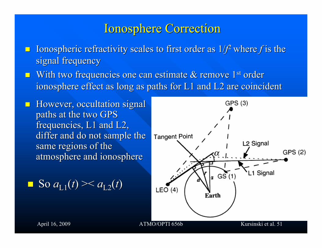
Ionosphere CorrectionIonosphere Correction Ionospheric Ionospheric refractivity scales to first order as 1/refractivity scales to first order as 1/ff2 2 where where ff is the is the

signal frequencysignal frequency With two frequencies one can estimate & remove 1With two frequencies one can estimate & remove 1stst order order

ionosphere effect as long as paths for L1 and L2 are coincidentionosphere effect as long as paths for L1 and L2 are coincident

So So aaL1L1((tt) >< ) >< aaL2L2((tt))

However, occultation signalHowever, occultation signalpaths at the two GPSpaths at the two GPSfrequencies, L1 and L2,frequencies, L1 and L2,differ and do not sample thediffer and do not sample thesame regions of thesame regions of theatmosphere and ionosphereatmosphere and ionosphere


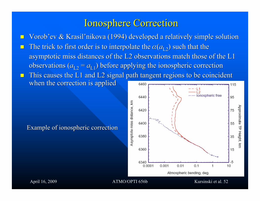
VorobVorob’’ev ev & & KrasilKrasil’’nikova nikova (1994) developed a relatively simple solution(1994) developed a relatively simple solution The trick to first order is to interpolate the The trick to first order is to interpolate the ((aaL2L2) such that the) such that the

asymptotic miss distances of the L2 observations match those of the L1asymptotic miss distances of the L2 observations match those of the L1observations (observations (aaL2L2 = = aaL1L1) before applying the ) before applying the ionospheric ionospheric correctioncorrection

This causes the L1 and L2 signal path tangent regions to be coincidentThis causes the L1 and L2 signal path tangent regions to be coincidentwhen the correction is appliedwhen the correction is applied

Ionosphere CorrectionIonosphere Correction

Example of Example of ionosphericionospheric correction correction

53

Refractivity ErrorRefractivity Error

Fractional error in refractivity derived by GPS ROFractional error in refractivity derived by GPS RO asasestimated in estimated in Kursinski Kursinski et al. 1997et al. 1997Considers several error sourcesConsiders several error sources

Solar max, low SNR Solar max, low SNR Solar min, high SNRSolar min, high SNR


GPSRO Temperature AccuracyGPSRO Temperature Accuracy

Temperature is proportional to Pressure/DensityTemperature is proportional to Pressure/Density So So TT/T /T = = PP/P /P - - // Very accurate in upper troposphere/lower troposphere (UTLS)Very accurate in upper troposphere/lower troposphere (UTLS)

SolarSolar max, low SNRmax, low SNR Solar min, high SNRSolar min, high SNR


Reducing the Reducing the ionospheric ionospheric effect of the solar cycleeffect of the solar cycle

With the currentWith the current ionospheric ionospheric calibration approach, a subtlecalibration approach, a subtlesystematic systematic ionospheric ionospheric residual effect is left in the bendingresidual effect is left in the bendingangle profileangle profile

ThisThis effect is large compared toeffect is large compared to predicted decadal climatepredicted decadal climatesignaturessignatures ~0.1K/decade~0.1K/decade

The residual ionosphere effect is due to an overcorrection ofThe residual ionosphere effect is due to an overcorrection ofthe the ionospheric ionospheric effecteffect

This This causes the causes the ionospherically ionospherically corrected bending angle tocorrected bending angle tochange sign and become slightly negative.change sign and become slightly negative.

This negative bending can be averaged and subtracted fromThis negative bending can be averaged and subtracted fromthethe bending angle profile to largely remove the biasbending angle profile to largely remove the bias

This idea needs further work but appearsThis idea needs further work but appears promisingpromising


Upper Boundary ConditionsUpper Boundary Conditions

We have two upper boundary conditions to contend with:We have two upper boundary conditions to contend with:the Abel integral and the hydrostatic integral.the Abel integral and the hydrostatic integral.

For the Abel, we can either extrapolate the bending angleFor the Abel, we can either extrapolate the bending angleprofile to higher altitudes or combine the data withprofile to higher altitudes or combine the data withclimatological climatological or weather analysis informationor weather analysis information

Hydrostatic integral requires knowledge of pressure nearHydrostatic integral requires knowledge of pressure nearthe the stratopausestratopause. Typical approach is to use an estimate of. Typical approach is to use an estimate oftemperature combined with refractivity derived from GPStemperature combined with refractivity derived from GPSto determine pressure.to determine pressure.

Problem with using a climatology is it may introduce a biasProblem with using a climatology is it may introduce a bias Also a basic challenge is to determine, based on the dataAlso a basic challenge is to determine, based on the data

accuracy, at what altitude to start the accuracy, at what altitude to start the abel abel and hydrostaticand hydrostaticintegralsintegrals


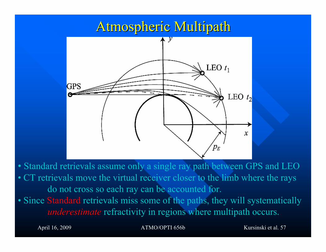
Atmospheric Atmospheric MultipathMultipath

• Standard retrievals assume only a single ray path between GPS and LEO• CT retrievals move the virtual receiver closer to the limb where the rays

do not cross so each ray can be accounted for.• Since Standard retrievals miss some of the paths, they will systematically

underestimate refractivity in regions where multipath occurs.


Existence & Mitigation of Atmospheric Existence & Mitigation of Atmospheric MultipathMultipathFor atmospheric multipath to occur, there must be large vertical refractivity gradients that vary rapidly with height with substantial horizontal extentOne expects multipath in regions of high absolute humidity

0.1 1 10

200

300

400

500

600

700

800

900

1000

Pw*

L = 3000km

L = 100 km

L = 50 km

Partial pressure of water vapor (mb) at equator

Pre

ssu

re (

mb

)

Saturation vaporSaturation vaporpressurepressure

Moving the receiver closer to the limb reduces the maximum altitude at whichmultipath can occur but it does not eliminate ray crossings

TAO,Kursinski et al., 2002

Max alt at which MP can occurMax alt at which MP can occurdue to a 100 m thick 100% due to a 100 m thick 100% relrel..hum. water vapor layer as ahum. water vapor layer as afunction of receiver distance tofunction of receiver distance tolimb, Llimb, L


Super-refractionSuper-refractionSuper-refraction: when the vertical refractivity gradient becomes so large that the radiusSuper-refraction: when the vertical refractivity gradient becomes so large that the radius

of curvature of the ray is smaller than the radius of curvature of the atmosphere,of curvature of the ray is smaller than the radius of curvature of the atmosphere,causing the ray to curve down toward the surface.causing the ray to curve down toward the surface.

No No raypath raypath connecting satellites can exist with a tangent height in this altitude interval.connecting satellites can exist with a tangent height in this altitude interval.–– A signal launched horizontally at this altitude will be trapped or ductedA signal launched horizontally at this altitude will be trapped or ducted–– This presents a serious problem for our This presents a serious problem for our abel abel transform pairtransform pair

Super-refractive conditions occur when theSuper-refractive conditions occur when therefractivity gradientrefractivity gradient dNdN//drdr < -10 < -1066//RRcc, where, where RRcc is isthe radius of curvature of the atmosphere;the radius of curvature of the atmosphere;–– CriticalCritical dN dN//drdr ~ -0.16 N-units m ~ -0.16 N-units m-1-1

Figure shows Figure shows raypathsraypaths in the coordinate system with in the coordinate system withhorizontal defined to follow Earthhorizontal defined to follow Earth’’s surfaces surface

Ducting layer in Figure extends from 1.5 to 2 kmDucting layer in Figure extends from 1.5 to 2 kmaltitudealtitude

No No raypathraypathtangent heightstangent heightsin this intervalin this interval


Super-refractionSuper-refractionThe vertical atmospheric gradients required to satisfy this inequality canThe vertical atmospheric gradients required to satisfy this inequality can

be found by differentiating the dry and moist refractivity terms of thebe found by differentiating the dry and moist refractivity terms of theNN equation: equation:

where where HHPP is the pressure scale height. is the pressure scale height.The three terms on the RHS represent the contributions of the verticalThe three terms on the RHS represent the contributions of the vertical

pressure, temperature, and water vapor mixing ratio gradients topressure, temperature, and water vapor mixing ratio gradients todN/drdN/dr..

PP gradients are too too small to produce critical gradients are too too small to produce critical NN gradients. gradients.Realistic Realistic TT gradients are smaller than +140 K/km needed to produce gradients are smaller than +140 K/km needed to produce

critical critical NN gradients gradientsPPww gradients can exceed the critical -34 mbar/km gradient ingradients can exceed the critical -34 mbar/km gradient in

the warm lowermost troposphere and therefore canthe warm lowermost troposphere and therefore canproduce super-refraction.produce super-refraction.

dN

dr = -

b1P

HPT -

b1P

T2

+2b2PW

T3

dT

dr +

b2

T2

dPW

dr


PBL schematicPBL schematic

0 2 4 6 8 10 12 140

0.5

1

1.5

2

2.5

Specific humidity (g/kg)

alti

tude (

km

)

a

290 295 300 305 310 315 320

Potential Temperature (K)

b

6380 6380.5 6381 6381.5 6382

asymptotic miss distance = n r (in km)

interval in which there are no raypath tangent heights

r1

r2

r3

a1

a2

d

150 200 250 300 3500

0.5

1

1.5

2

2.5

Refractivity

c

Super-refractionSuper-refraction

becomesbecomesimaginary withinimaginary withinthe intervalthe interval

222arn !

Feiqin Xie Feiqin Xie diddid his thesis here onhis thesis here ondeveloping a solution to thedeveloping a solution to thesuper-refraction problemsuper-refraction problem

Free troposphereFree troposphere

Mixed layerMixed layer

Cloud layerCloud layer


Occultation Features SummaryOccultation Features Summary

Occultation signal is a point sourceOccultation signal is a point sourceÞÞ Fresnel Fresnel Diffraction limited vertical resolutionDiffraction limited vertical resolutionÞÞ Very high vertical resolutionVery high vertical resolution

We control the signal strength and therefore have much moreWe control the signal strength and therefore have much morecontrol over the SNR than passive systemscontrol over the SNR than passive systems

ÞÞ Very high precision at high vertical resolutionVery high precision at high vertical resolution

Self calibrating techniqueSelf calibrating technique

ÞÞ Source frequency and amplitude are measured immediatelySource frequency and amplitude are measured immediatelybefore or after each occultation so there is no long term driftbefore or after each occultation so there is no long term drift

ÞÞ Very high accuracyVery high accuracy



Simple and direct retrieval concept

Þ Known point source rather than unknown distributedsource that must be solved for

Þ Unique relation between variables of interest and observations (unlike passive observations)

Þ Retrievals are independent of models and initial guesses

Height is independent variable

Þ Recovers geopotential height of pressure surfaces remotely completely independent of radiosondes



Microwave systemÞ Can see into and below clouds, see cloud base and multiple cloud layersÞ Retrievals only slightly degraded in cloudy conditionsÞ Allows all weather global coverage with high accuracy

and vertical resolution

Complementary to Passive Sounders

Þ Limb sounding geometry and occultation properties complement passive sounders used operationally

gps occultation introduction and overvie 16, 2009 atmo/opti 656b kursinski et al. 1 gps occultation...

Documents