grace, time-varying gravity, earth system dynamics and
TRANSCRIPT

3 April 2014
1 GRACE, time-varying gravity, Earth system 2 dynamics and climate change
3 B. Wouters1,2, J.A. Bonin3, D.P. Chambers3 , R.E.M. Riva4, I. 4 Sasgen5,6, J. Wahr2
5 1 Bristol Glaciology Centre, School of Geographical Science, Bristol, UK 6 2 Department of Physics, University of Colorado at Boulder, Boulder, Colorado, USA 7 3 College of Marine Science, University of South Florida, St. Petersburg, Florida, 8 USA 9 4 Department of Geoscience and Remote Sensing, Delft University of Technology,
10 Delft, Netherlands 11 5 German Research Centre for Geosciences, Potsdam, Germany 12 6 Department of Geosciences, The Pennsylvania State University, University Park, 13 USA
14 Abstract. 15 Continuous observations of temporal variations in the Earth’s gravity field have 16 recently become available at an unprecedented resolution of a few hundreds of 17 kilometers. The gravity field is a product of the Earth’s mass distribution, and these 18 data – provided by the satellites of the Gravity Recovery And Climate Experiment 19 (GRACE) – can be used to study the exchange of mass both within the Earth and 20 at its surface. Since the launch of the mission in 2002, GRACE data has evolved 21 from being an experimental measurement needing validation from ground truth, to a 22 respected tool for Earth scientists representing a fixed bound on the total change and 23 is now an important tool to help unravel the complex dynamics of the Earth system 24 and climate change. In this review, we present the mission concept and its theoretical 25 background, discuss the data and give an overview of the major advances GRACE has 26 provided in Earth science, with a focus on hydrology, solid Earth sciences, glaciology 27 and oceanography.

GRACE, time-varying gravity, Earth system dynamics and climate change 2
28 1. Introduction
29 Gravity is one of nature’s fundamental forces. Although most people tend to think of 30 gravity – or, more precisely, the gravitational acceleration g at the Earth’s surface – as 31 a constant of approximately 9.81 m/s2, it is not uniform around the globe. The Earth’s 32 rotation and its equatorial bulge cause deviations from the mean value of about half a 33 percent, which can be well predicted from theory. Because the Earth’s gravity field is 34 a product of its mass distribution, variations in the density of the Earth’s interior and 35 topography cause further regional deviations of a few tens of a millionth of g (Figure 1). 36 These are much harder to model, since this requires knowledge of the Earth’s structure. 37 However, mass transport in the interior is a slow process, so that these deviations can be 38 considered to be more or less constant on human timescales. Water, on the other hand, 39 is much more mobile than rock and its constant movement on the Earth’s surface and 40 in the atmosphere will cause changes in the gravity field on a wide range of time scales. 41 These variations are minute, but measuring them accurately means literally ’weighing’ 42 changes in the Earth’s water cycle and could help unravel the complex dynamics of 43 the Earth system and climate change. The list of possible applications of time-variable 44 gravity measurements is abundant: tracking changes in the water held in the major 45 river basins, observing variations in the hydrological cycle, measuring the ice loss of 46 glaciers and ice sheets, quantifying the component of sea level change due to transfer of 47 water between the continents and oceans, detection of water droughts and the depletion 48 of large groundwater aquifers due to unsustainable irrigation policies, and much more, 49 would all be possible. And even processes within the solid Earth would be measurable, 50 provided that they occur fast enough and their gravitational signal is strong enough 51 (e.g., mega-thrust earthquakes). As we will see, all of this and more has become reality 52 at a global scale since the launch of the Gravity Recovery And Climate Experiment 53 (GRACE) satellites. 54 Although the temporal gravity variations associated with the phenomena listed 55 above are extremely small (∼ 10−8m/s2), they can be measured with dedicated 56 instruments. Locally, time variations in gravity can be recorded accurately on the 57 ground by gravimeters [1], but global, satellite-based, measurements of time-variable 58 gravity have long been restricted to mapping large-scale variations only. These 59 early observations were mainly based on satellite laser ranging (SLR), which involves 60 measuring the position of satellites orbiting the Earth, with a precision of a few cm or 61 better. Such a high precision is obtained by emitting a laser pulse to a dedicated satellite, 62 covered with reflectors, and measuring the round-trip travel-time once the reflected pulse 63 is received. By collecting a sufficient amount of such position measurements, the orbit 64 can then be determined, which is for a large part determined by the Earth’s gravity 65 field. However, these satellites – such as the Laser Geodynamics Satellites (LAGEOS 66 [2]), launched in the 1970s and 1990s and still operational today – orbit the Earth at 67 a high altitude (∼6000 km) to minimize atmospheric drag. Because the sensitivity to 68 the Earth’s gravity field decreases with increasing altitude, the determination of time-

GRACE, time-varying gravity, Earth system dynamics and climate change 3
69
70
71
72
73
74
75
76
77
78
79
80
81
82
83
84
85
86
87
88
89
90
91
92
93
94
95
96
97
98
99
100
101
102
103
104
105
106
107
variable gravity with SLR is restricted to scales of typically 10,000 km [e.g., 3]. For a higher resolution, satellites at a lower altitude are required, such as the Challenging Minisatellite Payload (CHAMP; [4]) satellite, which allowed continental-scale gravity observations at seasonal periods (2000–2010), and in particular GRACE, the subject of this review article.
Like many space missions, GRACE had a long history of negotiation and deliberation before the satellites saw daylight. For at least two decades prior to its launch, the Earth Science community had been calling for a dedicated gravity satellite mission to provide an improved determination of the Earth’s static, global gravity field [e.g., 5, 6, 7, 8]. While that message had always been well received by NASA and other space agencies, the arguments had not been persuasive enough to lead to an approved mission. A combination of events in the late 1990’s changed that situation, and culminated in the acceptance of GRACE. One was the innovative GRACE measurement concept itself, which permits the recovery of monthly global gravity solutions of unprecedented accuracy down to scales of a few hundred km. Originally, though, the focus of GRACE was still to be on the static field. But officials at NASA, wondering about the possible scientific payoff of time-variable gravity measurements, commissioned the US National Research Council to undertake a study to look into this. Prior to that study, it was known that a mission like GRACE could recover the secular gravity changes due to vertical land-motion to useful accuracy, but there had been virtually no work done on the possible use of time-variable satellite gravity to study other processes. The resulting NRC committee, chaired by Jean Dickey, discovered a multitude of possible applications that were well suited to the expected spatial and temporal resolution of GRACE [9]. The proposed GRACE mission design and science plan were subsequently adjusted to focus on the time-variable field, rather than on the static field. The usefulness of these time-variable applications and their relevance to such a wide variety of Earth science disciplines, as well as the perceived ability of GRACE to recover those signals, were certainly among the factors that influenced the decision by NASA and DLR, the German space agency, to fund the mission. Relatively soon after funding was approved, the mission was launched on March 17, 2002, from Plesetsk Cosmodrome in Russia.
GRACE has lead to important new insights in many scientific fields, ranging from verifying the ’Lense-Thirring effect’ of general relativity [10] to the detection of a giant meteorite impact crater underneath the Antarctic ice sheet [11], to observing tropospheric density changes during geomagnetic storms [12], but it has greatly advanced our understanding of how masses move within and between the Earth’s subsystems (land, ocean, ice and the solid earth, in particular [13, 14]). Before reviewing the progress made in time-variable gravity research since the launch of GRACE, we briefly discuss the mission design, some essential equations and the GRACE data.

GRACE, time-varying gravity, Earth system dynamics and climate change 4
108
109
110
111
112
113
114
115
116
117
118
119
120
121
122
123
124
125
126
127
128
129
130
131
132
133
134
135
136
137
138
139
140
141
142
143
144
145
146
147
148
1.1. The GRACE satellites & data Although every satellite mission is a mammoth, complex operation, the basic principle of GRACE is beautiful in its simplicity. GRACE consists of two satellites in a low, near-circular, near-polar orbit with an inclination of 89◦, at an altitude of about 500 kilometres, separated from each other by a distance of roughly 220 kilometres along- track (Figure 2). The mission does not measure gravity directly with an active sensor, but is based on the satellite-to-satellite tracking concept, which tracks variations in the inter-satellite distance and its derivatives to recover gravitational information. Suppose the satellites approach a sizeable mass located on the Earth’s surface (e.g., an ice sheet): since the two GRACE satellites are separated by a certain distance, and the gravitational pull of the mass is inversely proportional to the squared distance to each satellite, the orbit of each of the satellites will be perturbed slightly differently. The leading satellite will be pulled slightly more towards the mass than the trailing one and the separation between the satellites will increase. Although these changes are minute – in the order of a few micrometres, or 1/100th of the width of a human hair – they can be measured by means of a dual-one way ranging system, the K/Ka band microwave ranging system (KBR). Non-gravitational forces, such as atmospheric drag will also alter the relative distance, and are accounted for using onboard accelerometer measurements. The orientation in space of the satellites are mapped by two star-cameras. Since the KBR measurements provide no information on the position in the orbit, the satellites are equipped with Global Positioning System (GPS) receivers so that their location is known.
From these data, called the Level-1 data, variations in the Earth’s gravity field can be recovered. This is generally done through an iterative procedure: first, an a-priori model of the Earth’s mean (static) gravity field in combination with other ’background’ force models (e.g., representing luni-solar and third body tides, ocean tides, the pole tide, etc.) is used to determine the orbit of both satellites. Importantly, the gravitational effects of ocean and atmosphere mass variations are removed from the measurements at this step using numerical models, because otherwise their high- frequency contributions would alias into longer periods and bias the results. Next, this predicted orbit is compared to the GPS and KBR observations and residuals are computed. Linearized regression equations are constructed, which relate the gravity field (more specifically, the spherical harmonic coefficients as we will see next) and other parameters to the residuals and are used to update the orbit. By combining data of a sufficiently long period – about a month, which guarantees a sufficient ground track coverage of the satellites – these equations can be used to relate the Level-1 observations to variations of the gravity field in a least square sense (see [15, 16]). The GRACE data are processed at three main science data centers, i.e., the Center for Space Research (CSR) and the Jet Propulsion Laboratory (JPL), both located in the USA., and the German Research Centre for Geosciences (GFZ) in Germany. Differences in the approaches of the processing centers lie in the background models used, the period

GRACE, time-varying gravity, Earth system dynamics and climate change 5
e
149
150
151
152
153
154
155
156
157
158
159
160
161
over which the orbits are integrated, weighting of the data, the maximum degree of the estimated gravity harmonics, etc. [17, 18, 19]. Other institutes are also providing independent gravity solutions nowadays, often based on alternative approaches [e.g., 20, 21, 22].
Next, we discuss the basic equations behind temporal gravity and the GRACE data. For the casual reader, it suffices to know the GRACE data generally are distributed as (Stokes) coefficients of spherical harmonic functions of degree l and order m, which can be related to variations in water height at the Earth’s surface. The maximum harmonic degree of the data depends on the analysis center, but in all cases it is sufficient to provide a spatial resolution of roughly 300 km.
The Earth’s gravitational field is described by the geopotential V . At a point above the Earth’s surface, with spherical coordinates radius r, co-latitude θ and longitude λ, it can be expressed as a sum of Legendre functions:
GM ( ∞ l ae l+1 V (r, θ, λ) =
ae
l=0 m=0 r
Plm(cos θ)(Clm cos mλ + Slm sin mλ)(1)
162
163
164
165
166
167
168
169
170
171
172
where G is the gravitational constant, M the mass of the Earth and ae denotes its mean equatorial radius. Plm are the Legendre polynomials of degree l and order m, and Clm and Slm are the spherical harmonic coefficients. The higher the order l, the smaller the spatial scale [see, e.g., 23, for a good introduction]. Note that as l increases, (ae/r)l+1, and consequently also variations in V , become smaller. Thus, satellites at lower altitudes r can better resolve small wavelength features.
Equation 1 may be used to define equipotential surfaces, i.e. surfaces of constant potential V . The equipotential surface that would best fit the mean sea level at rest is referred to as the geoid, which in turn can be approximated by an ellipsoid of rotation. The height difference between such a ’reference ellipsoid’ and the geoid is referred to as the geoid height and is approximated by Bruns formula:
V (R, θ, λ) − U 173 N =
γ (2) where U is the gravitational potential on the reference ellipsoid, equal to the constant potential of the geoid, and γ the normal gravity on the ellipsoid’s surface. The latter can be further approximated by GM/a2, so that in turn the geoid height can be approximated by [23]:
∞
174
175
176
177
178
179
N (θ, λ) ≈ ae Plm(cos θ)(Clm cos mλ + Slm sin mλ) (3) l,m
From this it follows that variations in the geoid height can be fully described by the spherical harmonic coefficients Clm and Slm, referred to as Stokes coefficients in geodesy. It is this set of coefficients that is estimated from the satellite measurements and distributed by the GRACE science teams every month as Level-2 data. The maximum degree l of the monthly Stokes coefficients lies between 60–120, which corresponds to a spatial resolution of roughly 150–300 km (20,000 km/l).

GRACE, time-varying gravity, Earth system dynamics and climate change 6
l
l
180
181
182
183
184
185
186
187
Geoid height is a commonly used unit in geodesy, but one more step is required to relate the Stokes coefficients to changes in (water) mass distribution, a more intuitive metric to most researchers studying the Earth’s water cycle. On monthly to yearly time- scales, changes in the Earth’s gravity field are primarily caused by redistribution of water in its fluid envelope, which all take place within a thin layer of a few kilometers near the Earth’s surface. In this case, (ae/r)l+1 in Equation 1 reduces to 1 and the anomaly in surface density (i.e., mass per area) can then be obtained using the following equation [see 24, for a step-by-step derivation]:
aeρe
∞ l 2l + 1
188 ∆σ(θ, λ) = 3
Plm(cos θ) l=0 m=0
1 + k1 ×(∆Clm cos(mλ)+∆Slm sin(mλ))(4)
189
190
where we included the symbol ∆ to indicate that we are dealing with time-variable quantities, and ρe is the average density of the Earth (5517 kg/m3). The load Love
191 numbers k1 [e.g., 25] account for deformation of the solid Earth due to the loading of
192
193
194
195
196
197
198
199
200
201
202
203
204
205
206
207
208
209
210
211
212
213
214
215
216
the mass anomaly on its surface, which will cause a small gravity perturbation as well. Units of ∆σ are typically kg/m2. Often, the surface density is divided by the density of water, which yields surface water height in meters water equivalent. An example of the surface height anomaly observed by GRACE for August 2005 is shown in Figure 3. When integrating ∆σ over an area, one obtains a volume estimate, usually expressed as km3 of water, or, equivalently, gigatonnes (Gt). One gigatonne equals 1012 kg, a sea level rise of 1 mm requires approximately 360 Gt of water.
The monthly GRACE Stokes harmonics are publicly available and can be downloaded from http://podaac.jpl.nasa.gov and http://isdc.gfz-potsdam.de. While the availability of GRACE data only as unfamiliar spherical harmonics originally slowed its application toward wider use by non-geodesists, the data has more recently been made available in easier-to-use gridded format as well (http://geoid.colorado. edu/grace/grace.php or http://grace.jpl.nasa.gov/data/). Yet, as we will see later on, interpretation of these gridded maps is not always straightforward and requires some expertise.
Some researchers also derive regional mass anomalies directly from the Level-1 range-rate data. In a method originally developed to study the gravity field of the moon, point masses or regional uniform mass concentrations (’mascons’) are spread over the Earth’s surface. The gravitation acceleration exerted by each mascon is then expressed as a sum of spherical harmonic functions so that the effect on the GRACE orbit can easily be computed. Each mascon is then given a scaling factor which is adjusted to give the best fit to the regional KBR observations [e.g., 26, 27]. Although this approach is computationally much more demanding, it has certain advantages, e.g., regional solutions can be obtained and certain constraints can be applied between neighbouring mascons to reduce the leakage problem, as discussed below.

GRACE, time-varying gravity, Earth system dynamics and climate change 7
217
218
219
220
221
222
223
224
225
226
227
228
229
230
231
232
233
234
235
236
237
238
239
240
241
242
243
244
245
246
247
248
249
250
251
252
253
254
255
256
257
1.2. Handling the GRACE data The first GRACE science results were published about two years after the mission launch [28, 29]. Many geophysical features – such as the seasonal change in water storage in the Amazon river system – were readily recognizable, but surprisingly, the maps of surface water height showed distinctive North-South striping patterns (Figure 3a). Although it had been anticipated during the mission design phase that the higher degree Stokes coefficients (i.e., small spatial scale) would have larger errors than the lower degrees (large spatial scale), such – clearly unphysical – striping had not been foreseen. The origin of these stripes lies in the orbit geometry of the GRACE mission [e.g. 30, 31]. The gravity field is sampled using the variations in the along-track distance between the two satellites, which circle the Earth in a near-polar orbit. As a result, the observations bear a high sensitivity in the north-south direction, but little in the east- west direction. Errors in the instrument data, shortcomings in the background models used to remove high-frequency atmosphere and ocean signals, and other processing errors will consequently tend to end up in the east-west gravity gradients. Since the release of the first GRACE data, methods to process the satellite data have improved and new ocean and atmosphere models allow for a better removal of high-frequency variability signals from the observations. This has lead to new, reprocessed GRACE solutions, which contain significantly less noise than earlier releases [32], as illustrated in Figure 3. Yet, although much reduced, the North-South striping problem persists.
Several methods have been developed to reduce the effect of noise in the GRACE data. One technique converts the global spherical harmonics into a local time series and then averages the observations over a larger, pre-determined region, such as river or drainage basins. If the area is sufficiently large – larger than the spatial decorrelation scale of the noise – the noise will tend to cancel out. Based on this concept, [33] formulated a ’basin averaging approach’ which aims to isolate the signal of individual regions while minimizing the effects of the noise and contamination of signals from the exterior. The ’basin averaged’ time series of the surface water anomalies can then be analyzed or compared to regional ground-based measurements.This has become a very common method of analysis with GRACE, especially in hydrological studies (see section 2).
Another straightforward and very commonly applied approach reduces the noise in the GRACE observations by smoothing the data. In the spectral domain, this means weighting the Stokes coefficients depending on the degree l, with a lower weight given to the noisier, higher degree Stokes coefficients. In the spatial domain, this is equivalent to convolving the GRACE maps with a smoothing kernel. A popular kernel is the Gaussian, bell-shaped, function, which decreases smoothly from unity at its center to zero at large angular distances (Figure 4) and is characterized by its smoothing radius, i.e., the distance on the Earth’s surface at which the kernel value has decreased to half the value at its center [34, 24]. As the smoothing radius increases, the higher degree Stokes coefficients are damped more strongly and the noise in the GRACE data

GRACE, time-varying gravity, Earth system dynamics and climate change 8
258
259
260
261
262
263
264
265
266
267
268
269
270
271
272
273
274
275
276
277
278
279
280
281
282
283
284
285
286
287
288
289
290
291
292
293
294
295
296
297
298
299
is reduced (Figure 5a-c). Unfortunately, using a large smoothing radius also means that the true, geophysical signals are damped and are smeared out over large regions, hindering a straightforward interpretation of the GRACE observations.
The Gaussian kernel has an isotropic character, i.e., it is independent of orientation, but as discussed above, the noise in the GRACE data has a strong non-isotropic North-South character. Non-isotropic filters have been developed [35, 36], but these generally still require a large smoothing radius to remove all stripes in the GRACE maps. A closer inspection of the GRACE Stokes coefficients by Swenson and Wahr [37] revealed that striping patterns could be traced back to correlated errors in the Stokes coefficients of even and odd degree l, respectively. This opened the door to more advanced post-processing methods which allowed a further increase of the spatial resolution of the GRACE data. To reduce the intercoefficient correlation, Swenson and Wahr [37] fit a quadratic polynomial in a moving window to the Stokes coefficients of even and odd degrees separately (for a fixed order m) and removed this from the original Stokes coefficients. Other methods apply principal component analysis on the Stokes coefficients [38] or use the full variance-covariance matrix of the Stokes coefficients [39, 40] to decorrelate the GRACE solutions. These advanced postprocessing methods have lead to a reduction of noise in the GRACE data of 50% and more [Figure 6; 41].
Unfortunately, the limited resolution of the GRACE data and the required post-processing means that the observations do not represent point-measurements. Additionally, any type of post-processing filter or during-processing constraint which reduces GRACE errors can also reduce local signal amplitude [42, 43, 44, 45]. So, when studying a specific region, one cannot simply take the average of the GRACE observations over that region. Besides the signal attenuation, leakage effects will bias such a simple average: due to the low resolution, water mass variations in neighbouring areas will spill into the desired region, while part of the signal of interest will spread outside the region. Leakage is particularly problematic in regions of high spatial variability in surface water storage patterns, as well as along coastlines where smoothing with the ocean’s far smaller signal notably damps the apparent hydrological signal. Rescaling is commonly used to remedy the signal loss caused by post-processing and the transformation of point-source signals to a finite number of spherical harmonics (e.g., up to degree and order 60). To compute a rescaling parameter, a model is made with higher spatial resolution than GRACE, then transformed to the limited set of spherical harmonics that GRACE uses and post-processed identically to GRACE. A ratio of the original model to the post-processed model signal amplitude is called the rescaling parameter. Assuming that the model reasonably represents the spatial pattern of the true signal, this ratio can act as a multiplier to upscale or downscale the actual post-processed GRACE data and counter the amplitude damping effect seen as leakage. Typically, the rescaling has been done on a basin scale [e.g., 46], though recently Landerer and Swenson [44] have tested and released a 1◦ × 1◦ mapped version of GRACE with rescaling and rescaling errors included, specifically focused at hydrologists. Nonetheless, limitations and inaccuracies at short spatial scales remain a

GRACE, time-varying gravity, Earth system dynamics and climate change 9
300
301
302
303
304
305
306
307
308
309
310
311
312
313
314
315
problem, especially as the focus moves to smaller and smaller basins. In addition to spatial limitations, GRACE’s typical monthly sampling rate also
limits its ability to estimate signals that act at shorter than seasonal time scales, though it handles annual and longer-term signals well. Recently, a few sub-monthly signals have been produced [47, 48, 49, 50, 20, 26], but the remaining delay between observation and data delivery makes real-time assessments (for which they would be most desired) impossible. Typically, increasing the temporal resolution of the GRACE time series means accepting an increased noise level in the signal, since the ground track coverage becomes less dense. Various types of constraints can ameliorate the difficulty, but not eliminate it entirely – and these constraints often alter the signal strength along with that of the noise.
After these introductory sections, we will now give an overview of the Earth Science applications of GRACE in the fields which have most benefited from this unique new set of time-variable gravity observations (hydrology, solid Earth sciences, glaciology and oceanography). Each section discusses the unknowns before GRACE was launched, the major scientific advances the mission provided and its limitations.

GRACE, time-varying gravity, Earth system dynamics and climate change 10
316 2. GRACE and Hydrology: A bound on terrestrial water storage
317
318
319
320
321
322
323
324
325
326
327
328
329
330
331
332
333
334
335
336
337
338
339
GRACE’s ability to accurately measure sub-yearly to decadal-trend mass changes on the global and regional scales has made it a unique data source for hydrology and hydrological modeling. Prior to the GRACE mission, total terrestrial water storage (TWS) changes over land could not be measured over significant spatial or temporal scales. Instead, the focus was on individual pieces of TWS: groundwater (GW), near-surface and deep soil moisture (SM), surface water (SW), snow-water equivalent (SWE) and ice, and water contained within biomass (BIO). These subsections of the terrestrial water storage were measured via in situ systems or other satellites, and/or were modeled from basic principles. However, the difficulty and expense of establishing and maintaining reliable in situ observation systems is significant, especially over large and remote areas and for long periods of time. Where observation coverage is good, in situ measurements have focused on particular sub-sections of the water signal, resulting in, for example, excellent coverage of near-surface soil moisture and groundwater, but no knowledge at all of surface water. Hydrological models also reflect this, often lacking one or more components of water storage in their computations. A growing selection of remote sensing hydrologic tools exist, but few have long data records and none besides GRACE see signals below a shallow subsurface layer.
GRACE’s ability to measure the sum of all hydrologic components in the water column, over the entire planet, at monthly intervals has proven a bounty for large- scale hydrological researchers. Two parallel techniques exist when using GRACE for hydrologic purposes. The first, as suggested above, is to solve for changes in TWS directly, based on changes (∆) in some or all of the individual components of water storage listed above:
340 ∆TW S = ∆GW + ∆SM + ∆SW + ∆SW E + ∆BIO (5)
341
342
343
344
345
346
347
348
349
350
351
352
353
354
This technique is particularly valuable in combination with observed data for some of the terms on the right-hand side of equation 5, using GRACE to give the ∆TWS sum. The second common technique is to consider the processes which cause changes in terrestrial water storage, principally precipitation (P), evapotranspiration (E), and runoff/discharge (R):
∆TW S = P − E − R (6)
This is often useful for modelers, who can use GRACE’s estimate of terrestrial water storage changes to bound their estimates of P, E, and/or R, oftentimes in combination with other observations of those same variables. The combination of P-E can also be estimated based on atmospheric anomalies, if the change in water vapor and the divergence of the atmospheric moisture transport are known. Whether using equation 5 or 6, GRACE measurements present a mathematical bound which did not exist before.
Besides the main limitations of GRACE mentioned in the introduction, such as the need for smoothing and post-processing, the limited spatial resolution and leakage

GRACE, time-varying gravity, Earth system dynamics and climate change 11
355
356
357
358
359
360
361
362
363
364
365
366
367
368
369
370
371
372
373
374
375
376
377
378
379
380
381
382
383
384
385
386
387
388
389
390
391
392
393
394
395
396
of GRACE signal into and out of the desired region, a major complexity with using GRACE for hydrologic purposes is inherent in its definition: GRACE measures the entire water column as one measurement. This makes separation into hydrologic constituents complicated, requiring combination with other hydrologic products, all of which have their own limitations and errors. The differing spatial and temporal scales between GRACE (a global, monthly product) and in situ data such as river or well gauges (point-source measurements which are non-uniform in space and time) makes exact comparisons and combinations difficult. Complications can also arise if non-hydrologic mass signals, such as alterations of mass in the atmosphere or solid Earth or leakage from the nearby ocean, also occur in the region, a particular problem given that models to correct for such signals are not perfect. The lower noise levels of GRACE RL05 [32] are expected to reduce many of these problems, but the general design of the GRACE mission means that they cannot be completely eliminated.
The use of GRACE by hydrologists has gone through two historical stages: validation and full utilization. For several years after the 2002 launch of GRACE, the focus was on using hydrological models and observational data to determine the accuracy of GRACE itself. Many of the initial comparisons were qualitative and large- scale. Various researchers [27, 26, 51, 28] created side-by-side comparisons of GRACE with hydrological models, as in Figure 7a, or otherwise noted that the dynamically- active regions seen by GRACE matched where hydrological models and our previous understanding of weather and climate placed them. Others [52, 53, 29] compared GRACE results to hydrological models across large basins (Figure 7b) and noted that both amplitude and phase were typically close. Later, EOF analyses were used to better quantify the similarities [54, 55]. The images shown here use the most recent CSR RL05 GRACE series from February 2004 to January 2012, but even one or two years of RL01 GRACE were sufficient to verify the general accuracy of GRACE in large, hydrologically-active regions.
Once several years of GRACE data had been garnered, hydrological GRACE papers became more in-depth and quantitative, using models, in situ data, or both to verify the general accuracy of GRACE and estimate the combined error in GRACE and their other data sources. A fine early example is Swenson et al. [56], who made use of a widespread in situ well and soil moisture network in the US state of Illinois. Based on prior knowledge, they assumed that the dominant terms in equation 5 in Illinois were groundwater (GW) and near-surface soil moisture (SM), ignoring surface water, snow, and the effect of the biosphere. They smoothed and destriped three years (2003–2005) of GRACE RL01 data, took the significant gravitational signal associated with vertical land motion (see Section 3) into account, then used a basin average to compute the ∆TWS time series over the Illinois region. When they compared the GRACE ∆TWS to the sum of in situ ∆SM and ∆GW from wells, they found good agreement (Figure 8a). Seasonal amplitudes ranged between 5-10 cm depending on the year, while the RMS difference from the in situ ∆GW+∆SM was only 2 cm, much of which was likely caused by the 1.8 cm in estimated GRACE RMS errors. The three-year correlation between ∆TWS from

GRACE, time-varying gravity, Earth system dynamics and climate change 12
397
398
399
400
401
402
403
404
405
406
407
408
409
410
411
412
413
414
415
416
417
418
419
420
421
422
423
424
425
426
427
428
429
430
431
432
433
434
435
436
437
438
GRACE and ∆GW+∆SM from in situ measurements was 0.95. This was put forth as early evidence that seasonal hydrological signals seen by GRACE are reasonable. Additionally, Swenson et al. found that in Illinois, soil moisture and groundwater are of approximately equal magnitude, with soil moisture sometimes lagging the groundwater by a month or two (Figure 8b). This means that in order to compare with GRACE, estimates of both groundwater and soil moisture are needed, not merely one or the other, a finding which has been confirmed via terrestrial gravity measurements [e.g., 57]. Thus a model which ignores either one would be unable to represent the true terrestrial water storage well.
Unfortunately, groundwater is not predicted by several global hydrology models, including one of the more commonly-used: the Global Land Data Assimilation System (GLDAS, [58]). Moreover, it proved difficult to find other in situ systems of measurement for both groundwater and soil moisture over large areas. Rodell et al. [59] worked around this in the greater Mississippi basin by combining what they did have: in situ well measurements for groundwater, and soil moisture and snow-water equivalent estimates modeled by GLDAS. Rather than combining the in situ ∆GW with the modeled ∆SM+∆SWE and comparing to GRACE’s ∆TWS, they worked equation 5 backwards, solving for the ∆GW which the GLDAS model could not provide. They compared that to the in situ well measurements – which are not available in many areas of the world – for verification that ∆GW can be estimated in such a manner. Using two years of RL01 GRACE data (2002–2004), they demonstrated that the seasonal groundwater signal in the wider Mississippi basin can be estimated using GRACE terrestrial water storage and the SM+SWE from a model. However, when they repeated the same procedure for smaller subbasins of the Mississippi, they found that the technique failed to properly determine the seasonal well signal in basins smaller than about 900,000 km2. While well undersampling in the spatial domain and inaccurate assessments of well specific yields also provided serious concerns, the dominant error source in these smaller subbasins was assumed to be the RL01 GRACE product.
A similar study was performed across the US state of Oklahoma [60], and another over the High Plains Aquifer in the US [61]. The latter is particularly interesting in that it investigated water storage changes in a semi-arid region which is heavily irrigated using groundwater. It thereby touched on the socio-economic issue of water scarcity and large- scale human pumping for groundwater, something not considered by most large-scale hydrological models at the time. Strassberg et al. [61] averaged the RL01 GRACE fields into three-month seasons to better reduce noise, then compared to in situ groundwater data from 2719 intermittent wells in the area and modeled soil moisture estimates from NLDAS (North American Land Data Assimilation System). The groundwater and soil moisture signals were both large (5-7 cm maxima) and varied differently in time, with a clear seasonal signal in the groundwater but not in the soil moisture. They found a correlation of 0.82 between GRACE ∆TWS and the ∆GW+∆SM combination from the wells and model (above the 95% confidence level). A 3.3 cm RMS difference existed between the two series, largely caused by a greater estimated amplitude of ∆GW+∆SM

GRACE, time-varying gravity, Earth system dynamics and climate change 13
439
440
441
442
443
444
445
446
447
448
449
450
451
452
453
454
455
456
457
458
459
460
461
462
463
464
465
466
467
468
469
470
471
472
473
474
475
476
477
478
479
480
compared to GRACE, which Strassberg et al. [61] posited may be due to overestimation of ∆GW during local summer, when irrigation pumping is occurring. Despite the imperfect matching, this paper provided firm evidence that GRACE could add value to hydrological studies even in semi-arid regions where significant groundwater was being pumped for irrigation.
Even before the launch of GRACE, hydrological modelers were aware of imperfections in their models due to missing terrestrial water storage components. However, these errors of omission came into sharp relief when presented with independent GRACE results. For example, numerous researchers noted that while the spatial pattern of GRACE ∆TWS matched with models, the amplitude of the models was notably lower in many high-signal locations than what was seen with GRACE (the Amazon basin in Figure 7, for example) and occasionally differed slightly in phase as well (the Ganges basin in Figure 7). As the GRACE timespan lengthened, interannual variations and long-term slopes (Figure 9) were also found to differ locally [62, 54, 63]. Based on comparisons like those listed above, modelers began to trust GRACE more and started considering GRACE during their cycles of model improvements, to better tune their parameters [64, 65] or directly assimilate GRACE TWS into their models [66, 67].
Niu and Yang [68] wrote one of the earliest examples demonstrating GRACE’s use in improving hydrology models. They began with the standard NCAR CLM hydrology model and, based on in situ information and basic principles, altered it in five significant ways: (1) decreasing the canopy interception of precipitation, (2) altering the percolation rate through the soil column, (3) decreasing surface runoff and thus increasing infiltration of the surface, (4) reducing the rate of subsurface flow, and (5) increasing the permeability of frozen soil. These modifications were made ahead of time, then compared to GRACE, along with the original CLM model, as verification. They found that the alterations resulted in ∆TWS maps which more closely matched what GRACE saw than the original series did, demonstratably increasing the amplitude of the hydrology signal in high-signal areas like the Amazon and Zambezi basins. When looked at as basin-wide averages, the RMS difference between the modified model time series and GRACE was half or less the size of the RMS difference between the original model and GRACE over large cold basins (Ob), classic monsoon basins (Yangtze), and tropical rainforest basins (Amazon). The improvement continued to hold for basins on the order of 300,000 km2 , as well. This demonstrated not simply an improvement of one model over another, but also a method with which the independent GRACE data set could help determine the precise features of a model which cause improvement. In a later paper, Niu et al. [69] used similar techniques to determine an appropriate runoff decay factor for use with modeled snow.
Werth and Guntner [65] used GRACE to tune the WaterGAP Global Hydrology Model (WGHM) in a more statistically rigorous fashion. As they had only six years of GRACE data (2003–2008), they removed all long-term trends and focused only on seasonal and interannual variability. They performed sensitivity analysis on 21 model

GRACE, time-varying gravity, Earth system dynamics and climate change 14
481
482
483
484
485
486
487
488
489
490
491
492
493
494
495
496
497
498
499
500
501
502
503
504
505
506
507
508
509
510
511
512
513
514
515
516
517
518
519
520
521
522
parameters having to do with soil moisture, groundwater, surface water, snow-water equivalent, and biomass over 28 large river basins. After choosing the 6-8 most sensitive parameters in each separate basin, they used a Pareto-based multi-objective calibration scheme to balance the fit to GRACE’s ∆TWS and a secondary independent data set, river discharge. Their optimized results were then compared to the original model and explanations given for the differences seen. Overall, the calibrated model increased the variability of terrestrial water storage throughout the tropical and temperate regions while decreasing it in colder areas, making the calibrated model better match what is seen with GRACE. The parameters causing the changes depended largely on the basin. In tropical and temperate basins, a deeper rooting depth allowed for greater seasonal storage as soil moisture. In basins with widespread rivers, lower river flow velocities and larger runoff coefficients kept water in the rivers for longer, thus increasing and delaying the seasonal maxima in terrestrial water storage. In colder basins, raising the temperature of snow melt drove the snow to melt later, changing the phase of the signal more than the amplitude. Groundwater variability decreased in many arid and semi-arid regions due to increased evapotranspiration. The optimization findings also suggested a route forward to more improvements, such as using more than one soil moisture layer to prevent excessive drying from evaporation, decorrelating the soil moisture from GW in some areas, and testing to optimize parameters which set GW timing and river volume. Werth and Guntner [65] noted that while a few basins were relatively insensitive to this optimization scheme, in general, the use of GRACE in combination with river discharge rates improved the tuning of the WGHM.
A similar combined optimization scheme using river discharge and GRACE TWS was also used by Lo et al. [64] to tune their CLM model, and Zaitchik et al. [67] assimilated the two data sets along with groundwater observations into their GLDAS model for testing as well. Houborg et al. [70] assimilated GRACE into the Catchment Land Surface Model (CLSM), then applied that model to the specific problem of drought monitoring in North America. They first determined that the GRACE-assimilated model better matched in situ GW+SM data than did the original, un-assimilated CLSM model in most areas of the US. The addition of GRACE helped overcome various weaknesses in the CLSM, while the assimilation technique allowed the individual terrestrial water storage components of surface soil moisture, root-zone soil moisture, and GW to be separated (Figure 10), as they cannot be in GRACE alone. This combination of GRACE plus model could help improve the US and North American Drought Monitors in the future.
By around 2008, reductions in GRACE errors via release RL04, a longer time series, and increasing confidence with the data began allowing research into more varied subjects. (Guntner [71] is an excellent survey paper describing the state of GRACE hydrology at that time.) Local analyses of a wide selection of hydrological basins around the world have since been completed: in North America [72, 73, 74, 75], South America [76, 62, 77, 78, 79], Africa [80, 81, 82, 83, 84], Europe [85], Australia [86, 87, 88], Asia [89, 90, 91, 92, 93], and the Arctic [94, 95]. Several studies revolved around

GRACE, time-varying gravity, Earth system dynamics and climate change 15
523
524
525
526
527
528
529
530
531
532
533
534
535
536
537
538
539
540
541
542
543
544
545
546
547
548
549
550
551
552
553
554
555
556
557
558
559
560
561
562
563
564
the transference of water between the land and the ocean, particularly concerning the teleconnections of El Nino/La Nina [81, 62, 96, 97, 98, 99].
GRACE has also begun to be used in combination with GPS to estimate the short- term solid-earth deformations caused by variations in local hydrologic loading. Van Dam et al. [100] compared the vertical surface displacements derived from GRACE to GPS data from stations in Europe and found substantial differences in amplitude and phase for most sites. They attributed these differences to tidal aliasing in the GPS data, since the differences were largest at coastal sites. Steckler et al. [101] used GRACE along with river gauge data to estimate Young’s Modulus for the elastic loading of the lithosphere caused by monsoon flooding in Bangladesh. Kusche and Schrama [102] demonstrated how to combine GPS and GRACE into a single J2 series as well as a low-resolution (degrees 2-7 only) time series. Tregoning et al. [103] compared 10-day- averaged GPS measurements of crustal deformation with 10-day-averaged estimates of elastic deformation from GRACE. This demonstrated that a significant part of the non- linear GPS motions, particularly in the vertical direction, are caused by hydrological changes picked up by GRACE. After taking the monthly deformations from GRACE into account, Tesmer et al. [104] found a 0–20% reduction in GPS weighted RMS at 43% of their GPS stations and more than a 20% improvement at an additional 34%, percentages which improve if only the annual signal is considered. They noted that the GPS stations most likely to be harmed or not improve by the addition of GRACE were all located on islands or peninsulas – places where the deformational signal estimated from GRACE is likely smaller than the noise and leakage in GRACE, and thus where GRACE should not be expected to provide assistance. Valty et al. [105] computed the vertical displacement from loading at European GPS sites by combining GRACE with GPS and global circulation models, then used the ”three-cornered hat” technique to compute the errors from each contributing data source, assuming the errors in each data set are independent. They determined that, over large areas, GRACE’s precision was about twice that of GPS, and that such combined solutions for loading vertical displacement are not very sensitive to the specific choice of GRACE or GPS processing center.
Additionally, topics directly impacting people fell under study. A primary man- caused signal visible by GRACE is the depletion of freshwater via the pumping of underground aquifers, mainly for irrigation of farmland. This research is of considerable importance to regional planners, as groundwater is often slow to recharge, and extensive overdrawing of reservoirs could lead to costly land subsidence and future water shortages. Unfortunately, monitoring of groundwater use is limited and withdrawals for personal use and irrigation typically unrestricted. Additionally, most hydrological models (including GLDAS) do not model groundwater at all, or else model it without including anthropogenic withdrawal effects, or else (as WGHM) have yet to perfect their model of both natural and anthropogenic groundwater changes. Model estimates of trends, therefore, are often wrong in areas with significant groundwater reduction. Improving the modeled estimates of groundwater deplenishment by humans is thus a subject of

GRACE, time-varying gravity, Earth system dynamics and climate change 16
565
566
567
568
569
570
571
572
573
574
575
576
577
578
579
580
581
582
583
584
585
586
587
588
589
590
591
592
593
594
595
596
597
598
599
600
601
602
603
604
605
606
current effort by some hydrological modelers [106, 107, 108, 109]. GRACE’s estimate of variations in total terrestrial water storage is perhaps the only independent tool able to estimate the actual amount of water being withdrawn in comparison to the recharge by precipitation and flow each year.
Two dominant examples of this sort of research consider the highly-irrigated regions of northern India and interior California. Rodell et al. [91] focused on the depletion of GW in arid and semi-arid northern India, which is suspected to be larger than the rate of recharge. The Indus River plain aquifer is heavily drawn on to support agriculture and straddles the border between India and Pakistan, making land-based monitoring systems politically problematic as well as expensive. The use of GRACE for monitoring this region is made more complicated by the proximity of the Himalayas only about 100km to the northwest [110]. Rodell et al. [91] use the GLDAS hydrology model to estimate soil moisture in the region, then estimate ∆GW from the difference between GRACE ∆TWS and the modeled ∆SM from 2002–2008. Groundwater was shown to have a negative trend of about 4 cm/yr (Figure 11), which would cause a 0.33 m/yr fall in the local water table, on average. As precipitation was normal or even slightly greater than normal during the time period, and as measurable drops in in situ water levels have also been noticed, the mass loss is presumed to come predominantly from the drawing of groundwater for irrigation, rather than from natural causes. Additionally, they note that much of the water used from irrigation must be either evaporating or running off into rivers, rather than seeping through the soil back into the aquifer, which would be invisible to GRACE. In only six years, this region of India lost 109 km3 of its freshwater. If its consumption continues unabated, serious water shortages will cause hardship in future years. Several other studies have since confirmed these basic findings [110, 92].
A similar set of studies has been conducted by Famiglietti et al. [111] in the Central Valley of California. As with the Indus River aquifer, the aquifers underlying the Sacramento and San Jaoquin river basins are heavily pumped for agricultural irrigation. The southern San Joaquin basin, in particular, is a relatively dry area with little available surface water. Famiglietti et al. [111] first checked GRACE’s accuracy over this region by collecting in situ measurements of precipitation, evaporation, and streamflow runoff and comparing them to GRACE’s ∆TWS through the use of equation 5. They found excellent agreement at the seasonal scale, which gives confidence behind the ability of GRACE to measure accurate mass changes in this area. It also verified that the known wintertime droughts in 2006/07 and 2008/09 were large enough to be visible. Then, using in situ measurements of surface water, a local model of snow-water equivalent which is constrained by in situ measurements, and modeled soil moisture, they solved for groundwater using GRACE and equation 5. Over six years (2004–2010), local terrestrial water storage dropped by about 31 cm/yr with groundwater estimated to make up about 20 cm/yr of that loss. Over 80% of this occurred in the drier San Joaquin basin. However, Famiglietti et al. [111] note that prior to the drought beginning in winter of 2006/07, groundwater storage was roughly balanced, with neither large

GRACE, time-varying gravity, Earth system dynamics and climate change 17
607
608
609
610
611
612
613
614
615
616
617
618
619
620
621
622
623
624
625
626
627
628
629
630
631
632
633
634
635
636
637
638
639
640
641
642
643
644
645
646
647
648
gains nor decreases. Only after the onset of the drought did a clear negative trend set in. They note that, historically, this seems typical: regional farmers draw more GW for irrigation during dry times, but their non-drought-time withdrawals approximately balance with the natural recharge rate, leading to significant depletion of the aquifer over the long-term. GRACE could be used in such a manner, in combination with other measurements, to help create a long-term plan for sustainable water use in this sensitive and valuable region.
In addition to man-caused water storage change, more recent studies have focused on natural changes which could have profound impacts on human life. Extended floods and droughts, in particular, have been measured with GRACE. In areas with few in situ measurement systems in place, such as the Amazon [62, 77], GRACE is one of only a few remote systems capable of estimating the magnitude and duration of such weather events. While other remote systems like MODIS (Moderate Resolution Imaging Spectroradiometer) or Landsat measure surface water extent (but not depth), and TRMM (Tropical Rainfall Measuring Mission) observes rainfall in the tropics, none but GRACE give us information on what is happening under the surface over time. Even in places where effort has gone in to installing regular in situ measurement devices, GRACE provides assistance and a wide-view image of the situation. Leblanc et al. [87] used GRACE to measure a decade-long drought in southeastern Australia, for example. Australia has a good, though spatially limited, in situ measurement system for surface water and GW, but is dependent on models for estimates of soil moisture. Leblanc et al. [87] used equation 5 to verify that the yearly-averaged combination of their model and in situ data approximately summed to the ∆TWS seen by GRACE, with correlations of 0.92-0.94 for the 2003–2007 period. Groundwater was shown to account for the majority (86%) of the 13 cm ∆TWS loss seen by GRACE from 2002–2006, with soil moisture losing most of its available water during the early part of the drought. GRACE also measured the increase in mass associated with the precipitation increase in 2007, most of which is believed to have gone into replenishing the soil moisture rather than increasing surface flow. Leblanc et al. (2009) then used GRACE to calculate the severity of the drought in a quantitative way, relative to a 2001 threshold (Figure 12). Without requiring the use of any modeled data, they estimated the average total deficit volume during 2002–2007 to be about 140 km3, with a maximum severity of approximately 240 km3 during early 2007.
To summarize, GRACE has been demonstrated to be useful for measuring hydrological signals hard to estimate in other ways, including estimates of water storage change in poorly monitored regions; annual and longer-term GW change due to human activity; the relation of groundwater, surface water, and soil moisture to droughts and floods; the short-term elastic deformation of the Earth to hydrologic loading; and the teleconnections between land hydrology and oceanography. Limited spatial and temporal resolution make GRACE an imperfect product for some investigations, but overall, it has added to the body of hydrological understanding and will surely continue to do so for years to come.

GRACE, time-varying gravity, Earth system dynamics and climate change 18
649 3. GRACE and the solid Earth: an attractive look into the Earth’s interior
650
651
652
653
654
655
656
657
658
659
660
661
662
663
664
Most studies using GRACE data focus on processes occuring in the ocean, cryosphere or hydrosphere, which represent redistribution of water within a thin layer at the Earth’s surface. However, since the mean density of the Earth is about five times as large as that of water, GRACE measurements are especially sensitive to mass redistribution in the Earth’s interior. Given that GRACE cannot distinguish the source of the mass change (on or within the Earth), a correction for such solid Earth signals is critical if one wants to interpret the surface mass redistribution from GRACE correctly, in particular when one looks at long-term trends. However, these processes in the Earth’s interior are not just a source of noise: conversely, GRACE has also been used to improve our understanding of the solid Earth. Most processes in the Earth, like mantle convection and plate subduction, occur on long enough time scales to be considered as static over the GRACE period. Other processes, such as glacial-isostatic adjustment (GIA) lead to a long-term trend in the GRACE time series, whereas very large earthquakes, like the Sumatra-Andaman Earthquake, will typically show up as abrupt jumps in the gravity field. These two processes will be discussed next.
665
666
667
668
669
670
671
672
673
674
675
676
677
678
679
680
681
682
683
684
685
686
687
688
Glacial Isostatic Adjustment The Earth’s interior responds to changes of the load on its surface, for example, the retreat and re-advance of ice sheets, with viscoelastic deformation seeking to gain a new equilibrium state. This process, glacial-isostatic adjustment, induces changes in the Earth’s gravity field, the rotation of the Earth, surface geometry and sea-level height. On long time scales, the most important redistribution of ice mass is associated with the glacial cycles. Paleoclimatic records indicate that over the last 800,000 years – that is the period most relevant for GIA – glacial and interglacial epochs alternated with a period of about 100,000 years. This period coincides with the variation of the Earth’s orbital eccentricity, the Milankovich cycle of 95,800 yr, and several theories have been proposed about orbital forcing of the glacial cycles [e.g., 112, 113], yet their role in triggering internal feedbacks in the climate system are still far from understood [114].
Recent glacial cycles exhibit a glaciation phase, marked by a steady growth of ice during about 90–100 thousand years, followed by a rapid deglaciation phase that lasts only about 10–20 thousand years, with the Last-Glacial Maximum (LGM) about 21,000 years before present (BP). During the LGM, the Laurentide Ice Sheet, for example, covered large parts of the North American continent with ice of several km in thickness, depressing the Earth surface by hundreds of meters (schematically shown in Figure 13). The response of the Earth can be described by the flexure of an elastic plate, the lithosphere, with a thickness of about 100 km covering the viscoelastic mantle. Due to the high viscosity of the displaced mantle material, the adjustment to the ice retreat following the LGM is delayed, leading to surface displacement and gravity changes of the Earth on time scales of 10,000 years – a process still ongoing today. In the 18th century, Celsius [115] was among the first to collect evidence of falling sea-level and changing

GRACE, time-varying gravity, Earth system dynamics and climate change 19
689
690
691
692
693
694
695
696
697
698
699
700
701
702
703
704
705
706
707
708
709
710
711
712
713
714
715
716
717
718
719
720
721
722
723
724
725
726
727
728
729
730
coastlines related to GIA. Today, an imprint of GIA is clearly visible in the temporal trends of GRACE gravity-fields, for example in Fennoscandia and North America (as illustrated in Figure 14). GIA is also strongly present in Antarctica, but is less clearly visible in GRACE due to superposition with recent changes in continental ice, due to variations in glacier flow and snow accumulation.
GIA not only leads to deformation of the Earth’s surface, it also has a dominant impact on the sea-level relative to the Earth surface. As an ice sheet retreats, its gravitational attraction decreases and the sea level drops in its vicinity. In contrast, in regions with a GIA-induced increase of mass, the gravitational attraction increases and sea level tends to rise. In addition, the water volume changes – as ice is redistributed between the ocean and the continent – as well as the geometry of the ocean basin through deformation and flooding/falling dry of land in response to changing surface loads. These interactions between changes in the gravity field, deformation of the solid Earth and also disturbances in the Earth’s rotation vector will yield regional variations in relative sea level which are much more complicated than a uniform rise or fall of the ocean’s surface. This concept was already acknowledged in 1835 by Lyell [116], who studied rock formations formerly submerged in the ocean along the Baltic coast and concluded that, in this region, the relative sea-level ”is very different in different places”. Figure 15 shows geological evidence recording the viscoelastic, exponential- type fall of relative sea-level typical for GIA in the near-field of a former ice sheet, here the Fennoscandian ice sheet. Clearly, these regional variations needs to be considered in the interpretation of geomorphological indicators of past sea-level change, as well as in future projections. A unified theory describing the effects of sea-level changes on a Maxwell-viscoelastic, self-gravitating Earth was put forward by Farrell and Clark [117], building on the work of Woodward [118]; the related integral equation describing gravitationally consistent the mass redistribution between ice and ocean has become known as the sea-level equation (SLE) and it is now implemented in all state-of-the-art numerical models of GIA [e.g., 119, 120].
Modeling of GIA requires two main ingredients: an ice model and knowledge of the Earth’s structure. The former describes the loading and unloading of the Earth’s surface by the waxing and waning of the ice sheets. Constraints for extent and timing are typically taken from glacial trim lines, dating of moraines pushed forward by advancing glaciers and paleo-indicators of sea level far from GIA regions. For the Earth structure, the distribution of density and elasticity are taken from models based on seismological screening of the Earth, like the Preliminary Reference Earth Model (PREM) [121]. The Earth’s rheology can only be obtained from creep experiments of mantle rocks [122], but it was the investigation of GIA that first provided constraints on the Earth’s mantle viscosity [e.g., 123]. The ice model and Earth structure used in GIA models are strongly coupled: present-day uplift in a certain region can be due to a strong loss of ice after the LGM, but also by a moderate loss combined with a slow response of the solid Earth. The situation becomes even more complicated when a re-advance of the ice occurred. Ice and Earth models are therefore often iteratively adjusted until an optimal match is

GRACE, time-varying gravity, Earth system dynamics and climate change 20
731
732
733
734
735
736
737
738
739
740
741
742
743
744
745
746
747
748
749
750
751
752
753
754
755
756
757
758
759
760
761
762
763
764
765
766
767
768
769
770
771
772
found with present-day crustal deformation, e.g. from relative sea level indicators, and nowadays also GPS measurements and GRACE observations.
Theory and numerical models solving GIA, as well as the first model-based interpretations of observations in terms of the Earth’s viscoelastic structure, date back to the mid-1970s [e.g., 124, 125]. Since then, theoretical descriptions and their numerical implementation have continuously been advanced [e.g., 126, 127, 128, 129]. Current models now not only include the solution of the sea-level equation [130, 131], but also GIA-induced variations of the Earth’s rotation [e.g., 132, 133, 134, 135], two- and three- dimensional distributions of mantle viscosities [e.g., 136, 137, 138, 139, 140, 141, 142] and may allow for non-Newtonian [e.g., 143], composite rheologies [144] and compressible viscoelasticity [e.g., 145].
Over the instrumental period of about 100 yrs, the temporal behavior of GIA is well approximated by a linear trend, an exception being young and tectonically active provinces with a very low-viscous upper mantle, such as Alaska, Patagonia or the Antarctic Peninsula. This means that GIA is present in trend estimates from geodetic time series of surface deformation from GPS, tide-gauge and alimetry measurements of sea level, as well as measurements of the Earth’s rotational variations, classical leveling, surface-gravity and geocenter motion and in particular the gravity field changes from GRACE. Because of the long time scales associated with GIA, seasonal variations in the GRACE data related to e.g. the global hydrological cycle are hardly affected. But for the study of interannual and long-term mass trends, a correction for GIA needs to be subtracted from the GRACE observations. This is in particular the case for estimates of the integrated ocean mass change from GRACE where the GIA correction is of the same order of magnitude as the signal (see section 5) and for monitoring the mass balance of the ice sheets. As mentioned above, GIA models are often iteratively adjusted until an optimal agreement is reached with crustal uplift data. Unfortunately, uplift data is scarce for the polar ice sheets, due to the remote, hostile environment and the fact that much of the region is still covered by ice. Particularly, the poorly defined ice loading history and Earth rheology of the Antarctic region has been a key limitation in estimating the Antarctic ice-mass balance from GRACE [146, 147]. Since the uncorrected GRACE data over Antarctica show a trend close to zero, it is the GIA model that determines the contribution of the ice sheet to sea level change. Early GIA models showed widely varying GIA corrections, ranging from 113 to 271 Gt/yr [148], equivalent to a sea-level rise of 0.30–0.75 mm/yr. In the course of the 2000s, an increasing number of GPS stations have been installed in the interior of Antarctica as part of the POLENET project (www.polenet.org), complementing near-coastal GPS stations available since mid-1990s. Thomas et al. [149] re-assessed the ground motion at the available Antarctic GPS stations and found that the GIA models systematically overestimate the uplift recorded by GPS. These GPS data, together with new evidence from glacial geology that the West-Antarctic ice sheet lost significantly less ice since the LGM than previously thought, have lead to a revision of the GIA predictions. The most recent GIA corrections for the Antarctic continent are now in the range of 6 to 103 Gt/yr,

GRACE, time-varying gravity, Earth system dynamics and climate change 21
773
774
775
776
777
778
779
780
781
782
783
784
785
786
787
788
789
790
791
792
793
794
795
796
797
798
799
800
801
802
803
804
805
806
807
808
809
810
811
812
813
814
with a preferred value of ∼40–60 Gt/yr. This is about half the magnitude of earlier estimates, with the consequence of attributing substantially weaker mass loss to the Antarctic Ice Sheet [150, 146, 151, 147]. A substantial uncertainty remains concerning the GIA signal underlying the East-Antarctic ice sheet, and regional to local patterns of the solid Earth response.
For North America, however, GRACE has provided new insights into GIA. It has been argued that, at some stage, the Laurentide Ice Sheet consisted of two distinct ice domes located south-east and west of Hudson Bay [e.g., 152]. Tamisiea et al. [153] first analyzed the spatial GIA pattern in the GRACE trends for 2002 to 2005, and interpreted its signature in favour of such a glaciation scenario (Figure 14). Later van der Wal et al. [154] showed that part of these 5-year GRACE trend must be attributed to water storage variations south-east of Hudson Bay from summer 2003 to summer 2006, which can, for short time series, produce a gravity rate comparable to GIA. With two more years of GRACE data (August 2002 to August 2009), Sasgen et al. [155] confirmed that the pronounced two-dome GIA pattern is much reduced, yet a kidney-shaped anomaly is retained. These low positive GIA amplitudes may suggest early ice disintegrating within the Hudson Bay area, leading to comparably early floating of ice and hence de-loading of the continent. The problem of contamination by hydrological signals and noise in the GRACE data remains, currently hampering secure conclusions, although a combination of GRACE with other data sets, such as GPS [156] and terrestrial gravity data [157], may help to remedy this problem [63].
Paulson et al. [158] was the first to invert the GIA signal in the GRACE data over North America for the mantle viscosity using numerical modelling. Although the authors had to conclude that the GRACE and relative sea level data are insensitive to mantle viscosity below 1800 km depth, and that data can distinguish at most two layers of different viscosity, they demonstrated consistency between the inversion of GRACE and relative sea-level data. A new aspect GRACE brought into the study is the analysis of spatial patterns (’fingerprints’) of GIA associated with specific mantle viscosities. The inversion of the GIA signal magnitude remains somewhat ambiguous due to the trade-off between mantle viscosity and load as discussed earlier. Although this ambiguity is inherent also in the GRACE inversion, Paulson et al. [158] treat the (unknown) magnitude of the load as a free parameter that is adjusted to optimize the fit to the GRACE data. Then, the residual misfit depends mainly on the modelled and observed spatial pattern of the GIA that is mainly governed by the mantle viscosity. In this sense, GRACE represents a valuable new data set in addition to point-wise measurements like GPS, tide-gauges or sea-level indicators [122].
For the region of Fennoscandia, the ongoing adjustment has been monitored by GPS studies, most important the Baseline Inferences for Fennoscandian Rebound Observations, Sea Level and Tectonics (BIFROST) project [159, 160]. The results indicate a GIA-induced land-uplift at rates of up to 8 mm/yr close to the former load centre. Agreement between GRACE and the terrestrial data in terms of the spatial pattern and magnitude could be achieved after a robust multi-year GRACE trend was

GRACE, time-varying gravity, Earth system dynamics and climate change 22
815
816
817
818
819
820
821
822
available. Since the Fennoscandian GIA pattern is well recovered by GPS, the signal could be used to verify GRACE post-processing methods [e.g., 161]. As for North America, the separation of the GIA signal and that of hydrological mass variations remains the largest challenge and source of uncertainty. The first joint inversion of GRACE, GPS and tide gauge data was performed by Hill et al. [162], obtaining results that are consistent with previous models, but with an improvement in the spatial pattern, which again demonstrates the power of combining GRACE with other data sets.
823
824
825
826
827
828
829
830
831
832
833
834
835
836
837
838
839
840
841
842
843
844
845
846
847
848
849
850
851
852
853
854
Seismology A second area of solid Earth research where the time-variable measurements from GRACE have provided new insights is seismology. For the first time, widespread gravity changes induced by earthquakes can be observed directly [163]. Since the signal generated by most earthquakes is small in comparison with the background noise, only the largest seismic events, those with moment magnitudes Mw> 8 [164], can be successfully observed.
Such giant earthquakes are characterized by a displacement at the fault interface of several tens of meters, distributed over a surface of 300–1000 km along fault by 100–200 km across fault. They generate seismic waves that are detected around the globe, deform the earth’s surface by several meters close to the fault and at the centimeter-level a few thousand kilometers from the epicenter, and can generate significant tsunamis. Observations of those processes, such as seismic waves, surface deformation and tsunamis, are available within hours to days after each seismic event and can be used to constrain the earthquake kinematics and dynamics. However, most major seismic events occur at the boundaries of oceanic regions, so that the availability of direct observations of surface deformation (mainly by GPS) is spatially highly heterogeneous and mostly limited to one side of the fault (over neighbouring continental areas). Furthermore, seismic observations, which can be used to determine the locations and magnitudes of coseismic events beneath either the continents or oceans, are not sensitive to long-period postseismic motion. Since space-based gravity observations provide homogeneous coverage of the earth’s surface, and because they detect mass redistribution at scales of months and longer, they can reveal seismic information that would otherwise go unnoticed.
GRACE observations have improved our understanding of the largest earthquakes of the last decade, for two time-frames: the occurrence of a seismic event (coseismic phase) and the period after that (postseismic phase). There are three main postseismic processes: afterslip, poroelastic relaxation and viscoelastic relaxation. Afterslip is equivalent to an earthquake which occurs so slowly that it does not produce seismic waves, at time scales from a few hours to several weeks. This additional slip is usually located either on the same fault activated by the earthquake, or on deeper segments that have not released seismic energy. Poroelastic relaxation is related to the fact that the

GRACE, time-varying gravity, Earth system dynamics and climate change 23
855
856
857
858
859
860
861
862
863
864
865
866
867
868
869
870
871
872
873
874
875
876
877
878
879
880
881
882
883
884
885
886
887
888
889
890
891
892
893
894
895
896
sudden pore-pressure change induced by an earthquake can displace fluids contained in rocks, and the same fluids slowly return to their original location during a few months to years after the seismic event [165, 166]. Viscoelastic relaxation, which also plays a major role in the process of GIA discussed earlier, occurs in deeper parts of the Earth, where temperatures and pressures are so high that rocks behave as high-viscosity fluids (viscosities in the range 1018–1021 Pa s). In seismically active areas, this is typically the case below depths of 25-40 km. After an earthquake, the fault displacement (slip) causes an increase in stress at the bottom of the top brittle layer, and this stress is slowly released through viscous flow that can last for decades [167, 168].
In one of the first GRACE earthquake studies, Han et al. [169] used raw measurements of the inter-satellite distance changes (Level-1 data) to determine the co-seismic gravity signal from the 2004 Sumatra-Andaman event. Level-1 data are available relatively quickly, and allow for the isolation of sudden gravity changes from sub-monthly time series. Han et al. [169] concluded that among the major factors contributing to the gravity signal were density changes within the earth’s upper layers. Density changes have often been included in deformation models [170, 171], but they had not previously received much attention because dilatation effects play only a limited role in determining changes in the earth’s geometry, such as those observed by GPS and InSAR. However, when modelling the gravity changes observed by GRACE, the role of density variations is found to be as large as that of the displacement of rock material [169, 172]. This surprising result was later discussed in more detail by Cambiotti et al. [173] and Broerse et al. [174], who showed that the crucial effects of dilatation result from a combination of the large-scale sensitivity of GRACE and the presence of an ocean. The effects of dilatation on the deformation are small compared to the peak value, and so have little impact on geometrical observations, which tend to focus on the peak displacements. But those effects are spread over a large area, particularly for an earthquake with a large focal plane such as the Sumatra-Andaman event, and so can have a significant impact on large-scale measurements. The presence of an ocean is important because it dramatically reduces the density discontinuity at the solid earth’s surface (from about 2600 kg/m3 to 1600 kg/m3), and consequently reduces the gravity signal due to topographic changes (the Bouguer effect). This causes a further increase of the relative contribution of dilatation to the total gravity change. Other studies followed in 2007, showing that coseismic signals could be detected in pre-processed (Level 2) data, as well [175, 176, 177]. These studies opened the way to a broader use of GRACE measurements by the solid Earth community, since Level 2 data are freely distributed by the official GRACE processing centres. Mega-thrusts later became the object of intensive research, with the first results often published within only a few months after each event. This was the case, for example, for the 2010 Maule [178, 179] and the 2011 Tohoku-Oki [180, 181] earthquakes.
Apart from modelling issues (i.e., determining which processes need to be accounted for to reproduce GRACE observations), the main objective of using GRACE data to study coseismic deformation is to improve fault-reconstruction models. This is

GRACE, time-varying gravity, Earth system dynamics and climate change 24
897
898
899
900
901
902
903
904
905
906
907
908
909
910
911
912
913
914
915
916
917
918
919
920
921
922
923
924
925
926
927
928
929
930
931
932
933
934
935
936
937
938
important because more accurate fault models can help in understanding the relation between recent and past earthquakes in the same region [182], and to help isolate postseismic signals. This line of study has been addressed in several ways: first of all, existing fault models obtained from seismic and GPS data have been corroborated by GRACE data for the Sumatra-Andaman [e.g., 169, 177, 183], Maule [178, 179] and Tohoku-Oki [180, 184] events; secondly, GRACE data have been used to obtain Centroid Moment Tensor (CMT) solutions fthe or Sumatra-Andaman [173, 172], Maule [172], Tohoku-Oki [181, 185, 172] and the east Indian Ocean [172] earthquakes; finally, a few studies have used GRACE data to constrain a finite-fault model for the Maule [186] and Tohoku-Oki [187, 188] events.
As suggested by the number of studies listed above, perhaps the most interesting application of GRACE data in coseismic studies has been the inversion for CMT solutions. In a CMT description, a seismic source is represented by a point-like double- couple and characterized by a few fundamental parameters: seismic energy, fault plane orientation, and slip direction. Those parameters are enough to completely define the earthquake, as long as the point-source approximation is valid, i.e., as long as observations are taken far enough from the location of the seismic event. Because of the large-scale sensitivity of GRACE, CMT parameters are particularly well suited for an inversion of GRACE data, in what could be called ’GRACE seismology’.
This approach has been recently formalized by Han et al. [172], who applied it to all seismic events observable by GRACE up to that time (with the exception of the 2005 Nias earthquake, which can not be clearly separated from the co- and postseismic effects of the 2004 Sumatra–Andaman earthquake). Forward models of earthquake- induced gravity changes computed using the GRACE-inferred CMT parameters, are shown in Figure 16. Han et al.’s study has highlighted how the depth of a seismic event is crucial for establishing the importance of density changes, and hence for characterizing the pattern and amplitude of its gravity signature. It also showed that large trade-offs are present in the determination of seismic energy vs. dip angle, which is the inclination of the fault plane in the vertical direction, and of the direction of slip vs. strike angle, which is the orientation of the fault plane in the horizontal direction. An example of the energy-dip angle trade-off as a function of depth is shown in Figure 17. The implication is that GRACE data should best be viewed as supporting traditional seismic and geodetic data when inverting for earthquake mechanisms. Nonetheless, a CMT solution based on GRACE observations alone does provide an estimate of the total energy released during the first few weeks after the seismic event, including contributions from slow post-seismic processes. Those are hard to measure using other techniques and are therefore rarely observed. Results from Han et al. [172] support the presence a slow slip for the Sumatra- Andaman earthquake, as had been suggested earlier on the basis of seismic inversions of ultra-long periodic motion [189, 190]. A slow component has not been detected by GRACE for any other event.
The fact that GRACE provides large-scale spatial coverage of an earthquake area, raises the possibility of providing better constraints on postseismic processes than can

GRACE, time-varying gravity, Earth system dynamics and climate change 25
939
940
941
942
943
944
945
946
947
948
949
950
951
952
953
954
955
956
957
958
959
960
961
962
963
964
965
966
967
968
969
970
971
972
973
974
975
976
977
978
979
980
be obtained with sparse and unevenly distributed GPS measurements. This should be particularly true for viscoelastic relaxation, which is more widespread and longer- lasting than the effects of other processes, and therefore better suited to the spatial and temporal resolution of GRACE data. In addition, GRACE observations of postseismic deformation following large earthquakes can provide information about the mechanical properties (the rheology) of the entire upper mantle in the vicinity of the earthquake, and improvement over what can be learned from smaller events, since the depth sensitivity is roughly proportional to the earthquake size.
The first paper to address postseismic processes with GRACE data was Ogawa and Heki [175]’s study of the Sumatra-Andaman earthquake. After analyzing monthly data spanning 4 years (including 16 months after the event), they came to the conclusion that the observed recovery of the initial geoid depression could best be explained by the diffusion of water. In contrast to previous studies of poroelastic relaxation in the upper crust [e.g., 166], in this case the flow was predicted to have taken place in the upper mantle, where pressure and temperature conditions are so high that water is in a supercritical state. This study remains the only study, to date, to have addressed this process, in spite of the important role of water in the dynamics of the earth’s interior [191].
A few papers [183, 192, 193] have modelled the observed postseismic signal after the Sumatra-Andaman event as the result of viscoelastic relaxation. All studies agree that relaxation is characterized by a transient phase with fast flow followed by a slower steady-state phase. The simplest model that can represent such a process is a Burgers body, which has a mechanical analogue of a spring and dash-pot in parallel (Kelvin element), combined in series with a spring and dash-pot in series (Maxwell element). The Kelvin element accounts for most of the transient signal, usually localized in the shallow part of the upper mantle (the top 100–200 km), while the Maxwell element represents the steady-state deformation throughout the entire mantle, as is also assumed in GIA studies (discussed earlier in this section). Though such a mechanical model had already been suggested on the basis of GPS data alone [194], the availability of GRACE data made it possible to better discriminate viscoelastic effects from the effects of afterslip, which had also been proposed as a candidate explanation for the early postseismic phase [e.g., 195]. Since afterslip causes a deformation pattern similar to the coseismic signal, but with much smaller amplitudes, its identification requires the availability of accurate near-field measurements, which in the Sumatra-Andaman region were limited to a few GPS sites. Based on GRACE data alone, Han and Simons [183] strongly favoured viscoelastic relaxation as the primary postseismic mechanism for this event, with the possibility of a small role of afterslip in the first few days after the earthquake. Panet et al. [192], however, invoked the presence of a small amount of afterslip, on the basis of GRACE data and a few GPS sites at about 500–1000 km from the fault. Following a different approach, Hoechner et al. [193] started from GPS data to refine the coseismic model and to reduce the number of candidate postseismic models, and to estimate the optimal crustal thickness. Then, they used GRACE data to discriminate between two

GRACE, time-varying gravity, Earth system dynamics and climate change 26
981
982
983
984
985
986
987
988
989
990
991
992
993
994
995
alternatives, the combination of a Maxwell model and afterslip vs. a Burgers model, and found that the Burgers model provides a much better fit to gravity observations (Figure 18). Interestingly, this distinction was made possible by the fact that the two processes caused different patterns in the oceanic areas west of the Andaman islands, where no observations except those from GRACE were available.
When summarizing the role of GRACE data in improving our knowledge of the seismic cycle around the major subduction zones, we can safely say that results so far have already exceeded expectations. The accurate isolation of the coseismic signal has provided interesting information about slip occurring outside the classical seismic spectrum. However, the most important insights will likely originate from the study of postseismic deformation, which promises to highlight how stress evolves at scales of years to centuries, and how it is related to the recurrence of large earthquakes [196]. Since several years of observations are required to discriminate between different postseismic processes, there is still much to be learned by continuing to monitor the regions encompassing recent mega-thrusts events.

GRACE, time-varying gravity, Earth system dynamics and climate change 27
996 4. GRACE and the cryosphere: weighing the ice
997
998
999
1000
1001
1002
1003
1004
1005
1006
1007
1008
1009
1010
1011
1012
1013
1014
1015
1016
1017
1018
1019
1020
1021
1022
1023
1024
1025
1026
1027
1028
1029
1030
1031
1032
1033
1034
1035
Until not too long ago, ice sheets and, to a lesser extent, glaciers were considered to be rather inert systems, reacting only slowly to climate changes. The mass balance (MB) of an ice body – the temporal change of its mass M – can be expressed as:
dM
dt = MB = SM B − D (7) where SMB stands for surface mass balance (SMB), the sum of processes that
deposit mass on the surface (precipitation) and remove mass from the surface (runoff, drifting snow sublimation and erosion and surface sublimation), and D is the ice discharge across the grounding line, where we neglect the small basal melting of grounded ice and changes in the grounding line position [197]. In the vast, hostile polar environment, collecting sufficient in situ observations to constrain the MB of the ice sheets would be a gargantuan task and until about 20 years ago, estimates of the contribution of the ice sheets to sea level changes were necessarily based on extrapolation of sparse set of samples.
A giant leap forward in our understanding of the cyrosphere was made by the advent of satellite remote sensing. Despite the lack of missions specifically dedicated at observing the mass balance of the cryosphere, estimates of volume and mass changes were already made in the 1990s using satellite radar alimetry. These missions were typically designed to measure height changes over the ocean, which is relatively smooth compared to the outlet glaciers at the ice sheet’s edges. The rugged topography in these locations introduces an ambiguity in the determination of the echo position of the emitted radar beam: over flat surfaces the first returned radar pulse will be associated with the point beneath the satellite, but along-track variations in the ice surface will move this point away from nadir, so that the exact location of the measurement is unknown. This becomes especially problematic in the coastal regions, where outlet glaciers are located in narrow fjords with a cross section smaller than the radar footprint, typically a few km. Furthermore, depending on the properties of the surface snowpack, the radar pulse penetrates in the snow adding further ambiguity to the observed height variations [e.g., 198]. A dedicated ice altimetry mission, ICESat, launched in 2003 and decommissioned in 2010, countered these limitations by using a laser beam with a footprint of ∼70 m, sufficiently small to resolve narrow glaciers features and with minimal surface penetration. Unfortunately, due to degradation of the laser system, measurements were coarse in time (∼3 campaigns/yr) and space. The ESA Cryosat-2 mission, launched in 2010 and currently in orbit, uses a Synthetic Aperture Interferometric Radar Altimeter to accurately determine the angle of arrival of its radar pulse, which allows measurements even in very irregular terrain. Yet, a major problem, associated with all geometric measurements, remains: to relate surface elevation changes to mass changes, the observations need to be multiplied with the local surface density. This is less trivial than one would assume. In regions dominated by ice dynamics, the density used should be close to that of ice. In contrast, in areas where melt or

GRACE, time-varying gravity, Earth system dynamics and climate change 28
1036
1037
1038
1039
1040
1041
1042
1043
1044
1045
1046
1047
1048
1049
1050
1051
1052
1053
1054
1055
1056
1057
1058
1059
1060
1061
1062
1063
1064
1065
1066
1067
1068
1069
1070
1071
1072
1073
1074
1075
1076
1077
accumulation changes at the surface dominate, it should be roughly that of snow. In many regions, both mechanisms operate and an intermediate value is to be used. Snow and ice density vary by a factor 2-3, ranging from 100–200 kg/m3 for freshly fallen snow to 800-917 kg/m3 for ice, thus introducing a significant uncertainty in the mass change estimates from altimetry. Furthermore, spurious trends may be observed due to firn compaction (compaction of the top snow layer under its own weight), which are unrelated to mass changes and difficult to correct for as they depend on the snow properties, temperature variations and accumulation rate.
Another satellite-based method, the input-output method (IOM) combines measurements of the influx of surface mass with the outflux at the boundaries of the ice field. Surface mass balance (SMB) is taken from (regional) climate models which are driven by meteorological re-analysis data [e.g., 199]. The outflux by glacier discharge (D) is obtained by multiplying ice thickness with ice flow velocities at the glacier’s grouding line. These glacier velocities can be either obtained from in situ flow measurements or from space, e.g., using Interferometric Synthetic Aperture Radar (InSAR). This technique has a high spatial resolution and can map individual glacier systems, but combines two large quantities which both have large uncertainties. Furthermore, observations of ice flow are made typically only once a year, which does not allow the interpretation of rapid, month-to-month discharge events, and do not always cover all glacier systems.
Although GRACE has its own limitations (in particular its low resolution and sensitivity to glacial isostatic adjustment – see section 3), it measures mass changes directly with global coverage at monthly intervals and thus provides an excellent tool to monitor the cryosphere. Whereas seasonal changes in the GRACE maps are dominated by hydrologly, the strongest interannual changes and trends are found in glaciated areas (Figure 19). Relatively soon after the mission’s launch, the first mass balance estimates of the two major ice sheets became available. For the Greenland Ice Sheet (GrIS), most pre-GRACE studies suggested that the ice sheet had shifted from being in near- balance to losing mass in the mid-1990s [e.g., 200]. One of the first GRACE studies focusing on Greenland did indeed suggest a mass loss of 75 ± 26 Gt/yr for Apr. 2002– Jul. 2004 [46], although the time series of just two years was still too short to draw any firm conclusions. Indeed, interannual variability in the GrIS system lead to a wide band of mass balance estimates in the first few years of the GRACE mission. Extending the time series by two years, Velicogna and Wahr [201] found a radically different mass loss of -227±33 Gt/yr for Apr. 2002–Apr. 2006, with a 250% increase between the first and second half of the observation period. These estimates were based on the averaging-kernel method which calculates the average signal over a large area from the monthly spherical harmonic gravity fields [33] and did not allow a regional separation of the mass changes. Luthcke et al. [27] used the mascon approach to estimate mass changes directly from the intersatellite K-band range and range rate, which allowed the first interpretation at a drainage-system scale. A strong mass loss in the coastal regions was observed, which was only partly compensated by mass gain in

GRACE, time-varying gravity, Earth system dynamics and climate change 29
1078
1079
1080
1081
1082
1083
1084
1085
1086
1087
1088
1089
1090
1091
1092
1093
1094
1095
1096
1097
1098
1099
1100
1101
1102
1103
1104
1105
1106
1107
1108
1109
1110
1111
1112
1113
1114
1115
1116
1117
1118
1119
the interior of the ice sheet. Interestingly, this pattern mirrored the responses to climate warming as predicted by climate models, with increased precipitation at high altitudes and thinning at the margins due to warmer temperatures. The overall mass loss of Luthcke et al. [27] added up to 101±16 Gt/yr (2003–2005), mainly concentrated in the southeast and to a lesser extent in the northwest. The difference with the estimates of Velicogna and Wahr [201] likely arose from interannual variability and the relatively low signal-to-noise ratio of the first release of the GRACE spherical harmonic solutions. Indeed, when improved GRACE solutions became available, and with the help of post- processing filtering, Wouters et al. [202] showed that regional partitioning of the mass loss is feasible with the standard global spherical harmonics as well. For the entire study period (2003-2008) a mass loss of 179±25 Gt/yr was reported, but when considering the same observation period, results were consistent with Luthcke et al. [27]. This also implies that the mass loss in the last few years was comparatively larger, which was attributed to increased melt in the summer months. Again, the inland growth and coastal ablation was observed, with an epicenter in the southeast and increasing mass losses in the northwest. This spreading of the mass loss to the northwest (illustrated in Figure 20) was later confirmed in other studies [e.g., 203, 204, 205] and independently by GPS stations which recorded uplift of the Earth surface in response to the diminished ice load. In the same study, Khan et al. [206] also reported moderate deceleration of the southeast ice loss in 2006 based on GRACE and GPS observations.
As discussed earlier, GRACE only observes integral mass changes and cannot separate the individual components contributing to these changes. Van den Broeke et al. [197] successfully compared GRACE time series to IOM mass balance for the GrIS and found a good agreement between the two fully independent data sets. This validation of the IOM data allowed a further partitioning of the individual components (equation 7) contributing to the mass loss observed by GRACE. Roughly half of the mass loss was attributed to an increase in discharge (D), the other half to changes in SMB processes. In particular, it was shown that in the pre-GRACE era, a large positive anomaly in surface melt (and consequently runoff) had developed, balanced by an increase in precipitation. After 2004, precipitation levelled off, but runoff remained high, resulting in a negative SMB for the GrIS. The model also showed that approximately 30% of the meltwater refroze in the top firn layer of the ice sheet, thereby partly reducing the total mass loss, but also leading to a release of a significant amount of energy to the snowpack. Locally, temperatures of the firn layer were estimated to have increased by as much as 5 to 10 K. Sasgen et al. [203] continued along this path and found that the GRACE observations also agree with the IOM results at a regional scale. They revealed that the accelerating ice-mass loss along the west-coast of the ice sheet was a consequence of reduced SMB compared to the first few years of the GRACE observations, combined with an increase in glacier discharge. Furthermore, a good agreement was found between the regional GRACE mass balances and surface height changes from ICESat.
As the GRACE observational record lengthened, studies started to focus on interannual variations in the mass balance of the GrIS. A good example is the work
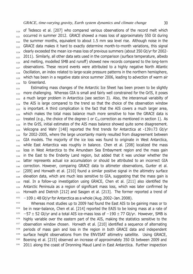
GRACE, time-varying gravity, Earth system dynamics and climate change 30
1120
1121
1122
1123
1124
1125
1126
1127
1128
1129
1130
1131
1132
1133
1134
1135
1136
1137
1138
1139
1140
1141
1142
1143
1144
1145
1146
1147
1148
1149
1150
1151
1152
1153
1154
1155
1156
1157
1158
1159
1160
1161
of Tedesco et al. [207] who compared various observations of the record melt which occurred in summer 2012. GRACE showed a mass loss of approximately 550 Gt during the summer months, equivalent to about 1.5 mm sea level rise. Although noise in the GRACE data makes it hard to exactly determine month-to-month variations, this signal clearly exceeded the mean ice-mass loss of previous summers (about 350 Gt/yr for 2002- 2011). Similarly, all other data sets used in the comparison (surface temperature, albedo and melting, modelled SMB and runoff) showed new records compared to the long-term observations. These record events were attributed to a highly negative North Atlantic Oscillation, an index related to large-scale pressure patterns in the northern hemisphere, which has been in a negative state since summer 2006, leading to advection of warm air to Greenland.
Estimating mass changes of the Antarctic Ice Sheet has been proven to be slightly more challenging. Whereas GIA is small and fairly well constrained for the GrIS, it poses a much larger problem in Antarctica (see section 3). Also, the interannual variabilty of the AIS is large compared to the trend so that the choice of the observation window is important. A third complication is the fact that the AIS covers a much larger area, which makes the total mass balance much more sensitive to how the GRACE data is treated (e.g., the choice of the degree-1 or C20 correction as mentioned in section 1). As in the GrIS, initial estimates of the AIS mass balance showed quite some disagreement. Velicogna and Wahr [148] reported the first trends for Antarctica at -139±73 Gt/yr for 2002-2005, where the large uncertainty mainly resulted from disagreement between GIA models. The majority of the ice loss was found to originate in West Antarctica, while East Antarctica was roughly in balance. Chen et al. [208] localized the mass loss in West Antarctica to the Amundsen Sea Embayment region and the mass gain in the East to the Enderby Land region, but added that it was unclear whether the latter represents actual ice accumulation or should be attributed to an incorrect GIA correction. However, comparing GRACE data to altimeter observations, Gunter et al. [209] and Horwath et al. [210] found a similar positive signal in the altimetry surface elevation data, which are much less sensitive to GIA, suggesting that the mass gain is real. In a follow-up investigation using GRACE, Chen et al. [211] also identified the Antarctic Peninsula as a region of significant mass loss, which was later confirmed by Horwath and Dietrich [212] and Sasgen et al. [213]. The former reported a trend of −109 ± 48 Gt/yr for Antarctica as a whole (Aug. 2002–Jan. 2008).
Whereas most studies up to 2009 had found the East AIS to be gaining mass or to be in near-balance, Chen et al. [214] reported the EAIS to be losing mass at a rate of −57 ± 52 Gt/yr and a total AIS ice-mass loss of −190 ± 77 Gt/yr. However, SMB is highly variable over the eastern part of the AIS, making the statistics sensitive to the observation window chosen. Horwath et al. [210] identified a sequence of alternating periods of mass gain and loss in the region in both GRACE data and independent surface height observations from the ENVISAT altimetry satellite. Using GRACE, Boening et al. [215] observed an increase of approximately 350 Gt between 2009 and 2011 along the coast of Dronning Maud Land in East Antarctica. Further inspection

GRACE, time-varying gravity, Earth system dynamics and climate change 31
1162
1163
1164
1165
1166
1167
1168
1169
1170
1171
1172
1173
1174
1175
1176
1177
1178
1179
1180
1181
1182
1183
1184
1185
1186
1187
1188
1189
1190
1191
1192
1193
1194
1195
1196
1197
1198
1199
1200
1201
1202
1203
of atmospheric reanalysis data attributed this mass gain to anomalously high snowfall in just two months, May 2009 and June 2010, due to atmospheric blocking events advecting moist ocean air towards the East Antarctic coast. The El Nino Southern Oscillation has also been linked to interannual variations in the mass balance of the AIS, in particular at the Antarctic Peninsula and in the Amundsen Sea sector, where the transport of atmospheric moisture from the ocean towards the continent is regulated by the Amundsen Low pressure system. Maximum correlation between the Southern Oscillation and interannual mass variations (∼ ±30 Gt) in these regions from GRACE were observed at a lag of 10 months [213].
Overall, when uncorrected for GIA, the apparent mass change in the GRACE time series is close to zero for Antarctica, so that the final result strongly depends on the method used to correct for GIA. Riva et al. [216] published a first AIS trend estimate which did not rely on GIA modelling, but separated ice-mass loss from GIA by combining the GRACE gravity data with ICESat surface elevation changes. This concept, based on earlier theoretical work of Velicogna and Wahr [217], relies on the fact that GRACE mass and ICESat elevation observations bear different sensitivities to GIA and ice-mass loss, respectively. Their GIA correction of 100±67 Gt/yr was considerably smaller than the correction used in Velicogna and Wahr [148] (176±72 Gt/yr). A wide uncertainty range remained, due to noise in the observations and the fact that firn compaction was neglected in the surface height trends, but this result suggested that the AIS GIA correction and consequently also the mass loss may have been overestimated so far. Indeed, as discussed in Section 3, a comparison of crustal uplift predicted by GIA models to vertical motion recorded by GPS stations indicated that the models systematically overestimated the GIA signal [149]. Recently developed GIA models suggest a GIA signal in the range of 6 to 103 Gt/yr, with a preferred value of ∼40–60 Gt/yr [218, 150, 151]. King et al. [146] applied the regional approach of Wouters et al. [202] to Antarctica, and, using the GIA correction of Whitehouse et al. [150], estimated an ice-mass change significantly lower than previous estimates (-69±18 Gt/yr for Aug. 2002–Dec. 2010), again concentrated along the coastal zone of the Amundsen Sea sector.
As is evident from the above overview, initially, mass loss trends reported in early GRACE studies disagreed by a factor of almost 2 for both ice sheets due to the different processing methods and, in particular, the time spans used. These early studies were based on only a few years of data, and surface mass balance for the GrIS and AIS may vary from one year to another by several hundred gigatonnes [219, 220], so adding just one year of measurements may change a trend substantially. Nowadays, as researchers have become more aware of the unique character of the GRACE data and the longer observations makes the statistics less susceptible to the choice of the time window, more recent estimates have converged. The Ice sheet Mass Balance Inter-comparison Exercise [221] compared GRACE mass balance estimates from six different research groups. A common time span was used (2003–2010) and all groups used the same GIA models, so that the differences between the estimates can be attributed to the data

GRACE, time-varying gravity, Earth system dynamics and climate change 32
1204
1205
1206
1207
1208
1209
1210
1211
1212
1213
1214
1215
1216
1217
1218
1219
1220
1221
1222
1223
1224
1225
1226
1227
1228
1229
1230
1231
1232
1233
1234
1235
1236
1237
1238
1239
1240
1241
1242
1243
1244
1245
source (the global Level-2 spherical harmonics provided by the GRACE science teams, or the ’mascons’ estimated directly from the Level-1 range-rate data) and the analysis scheme used to estimate the mass changes from the GRACE data. This showed that all estimates agree within their respective uncertainties, for both ice sheets. Trends differed by approximately ±10 Gt/yr between the six groups, which can be taken as the approximate current methodological uncertainty. For the GrIS, this is comparable to the uncertainty in the GIA correction, for the AIS, GIA remains the main source of uncertainty (see Section 3 for a discussion). At time of writing, mass loss of the GrIS stands at approximately -251±20 Gt/yr (Jan. 2003–Dec. 2012; update of Wouters et al. [222]). For the AIS, the numbers still depends on the approach used to correct for GIA and mass loss is nowadays in the range of -67±18 Gt/yr (Mar. 2003–Jul. 2012; update of King et al. [146]) to -114±23 Gt/yr (Jan. 2003–Sep. 2012; [151]). As is evident from Figure 21, the rate of mass loss of both ice sheets appears to have been steadily increasing since the launch of the GRACE satellites. Velicogna [223] found that the GrIS and AIS time series are indeed better characterized by a quadratic rather than a linear fit. This study reported an acceleration of -26±14 Gt/yr2 and -30±11 Gt/yr2 for Antarctica and Greenland, respectively, for 2002–2009 (fitting a α0 + α1t + 0.5α2t2 function, where α1 symbolises the trend and α2 the acceleration). Rignot et al. [224] extended the GRACE time series by one year and reported acceleration which were approximately 50% smaller (-13.2±10 Gt/yr2 for AIS and -17.0±8 Gt/yr2 for GrIS). These two studies used a slighly different approach to estimate the accelerations: fitting a quadractic to the GRACE mass anomalies (cummulative mass balance, M (t)) in Velicogna [223] versus fitting a linear trend to the monthlly mass balance values (dM/dt) in Rignot et al. [224], but this explains only a few Gt/yr2 of the differences. Adding another two years of data, Wouters et al. [222] found -21±13 Gt/yr2 and -25±9 Gt/yr2, respectively. Since acceleration estimates are unaffected by GIA (this slow phenomenon can be assumed to be approximately linear over the time period considered), this indicates that, again, the statistics are sensitive to the choice of the observation window and, to some degree, to the choice of data and processing [146, 225]. The high interannual variability in SMB makes the current GRACE record too short to robustly separate long-term accelerations from internal ice sheet variability. About 20 years of observations would be required to obtain an acceptable signal-to-noise ratio [222], highlighting the need for a follow-up GRACE mission.
GRACE has also provided important new insights in the mass balance of smaller ice caps and glaciers systems. Direct observations of glaciers are sparse, both in space and in time, because of the labour intensive nature and tend to be biased toward glaciers systems in accessible, mostly maritime, climate conditions. Approximately 60% of the in situ glacier mass balance records are from the smaller European Alps, Scandinavia and northwestern America [226]. Very large and less accessible glaciers, in contrast, are undersampled and lack continuous and uninterrupted observation series. Both problems can be overcome by GRACE, which provides global and continuous observations. Yet, as the spatial scale becomes smaller, the effect of noise in the GRACE data becomes

GRACE, time-varying gravity, Earth system dynamics and climate change 33
1246
1247
1248
1249
1250
1251
1252
1253
1254
1255
1256
1257
1258
1259
1260
1261
1262
1263
1264
1265
1266
1267
1268
1269
1270
1271
1272
1273
1274
1275
1276
1277
1278
1279
1280
1281
1282
1283
1284
1285
1286
1287
larger and validation of the GRACE observations of glaciers by independent methods becomes often desirable.
Much of the attention has focused on the glaciers in the (sub)Arctic region. In the Gulf of Alaska (GoA), airborne altimetry observations in the 1990s and early 2000s suggested a glacier mass loss of -96±35 Gt/yr for 1995–2001 [227]. This number was based on extrapolation of 28 profiled glaciers and the observations did not allow to resolve interannual variations. The first GRACE-based estimates confirmed the altimetry results, with trends of typically 100-110 Gt/yr in the first few years of the GRACE mission [∼2003–2005; 228, 229, 230]. However, the GRACE time series revealed substantial interannual variabilty in the mass budget of the GoA glaciers (see Figure 22): anomalously high snowfall in the winter of 2007 [230] was followed by high mass loss in 2009, which Arendt et al. [231] linked to the Mount Redoubt eruption in March of that year. The ash fall of the volcanic plume caused a decrease in the ice surface albedo in the GoA region, leading to a greater absorption of solar radiation and hence surface melt. They report a mass trend of -61±11 Gt/yr for 2004–2010, somewhat more negative than the -46±7 Gt/yr of Jacob et al. [110] for a slightly longer period (2003–2010). Interestingly, GRACE suggests that the neighbouring glaciers in Western Canada and USA are gaining mass at a moderate rate of a few Gt/yr (Fig. 22; [110, 232]), although the uncertainty due to GIA and leakage of hydrological signals is large for this region and in situ measurements indicate that these glaciers are actually losing mass [232].
Located northwest of the GrIS, the glaciers and ice caps of the Canadian Arctic Archipelago (CAA) hold about one-third of the global volume of land ice outside the ice sheets. Mass loss in the northern CAA was reported in the study of Wouters et al. [202]. A few years later, Gardner et al. [233] compared data from ICESat, GRACE and a regional climate model for 2004–2009 and found that all three data sets indicated a sharp acceleration of the mass loss occurring around 2007 (Fig. 22), mainly due to increased melt in response to higher air temperatures. About two-third of the ice loss (39±9 Gt/yr) was attributed to the northern part of the archipelago, while in the southern part, the melt (24±7 Gt/yr) was found to have doubled compared to its long- term value (11.1±1.8 Gt/yr for 1963–2008 [234]). Recently, GRACE data was also used to validate climate projections of a more advanced regional climate model in the CAA region, which indicates that the accelerated ice-mass loss will be sustained in the 21st
century [235]. Another region where glaciology has much benefited from the GRACE mission is
the Russian High Arctic. In-situ measurements are extremely sparse in this region, for example, Severnya Zemlya has been surveyed only three times (1957, 1958 and 1969) and no in situ surface mass balance measurements at all are available for Franz Josef Land [236]. Moholdt et al. [237] assessed the regional glacier mass budget for 2003– 2009 using ICESat and GRACE and found a small imbalance of 9.1±2.0 Gt/yr for this period, mainly due to ice loss in Novaya Zemlya. Comparable ice loss has been observed with GRACE in Iceland [∼-11 Gt/yr; e.g., 202, 110, 232] and Svalbard [-3 to -9 Gt/yr, depending on the observation window e.g., 202, 110, 232].

GRACE, time-varying gravity, Earth system dynamics and climate change 34
1288
1289
1290
1291
1292
1293
1294
1295
1296
1297
1298
1299
1300
1301
1302
1303
1304
1305
1306
1307
1308
1309
1310
1311
1312
1313
1314
1315
1316
1317
1318
1319
1320
1321
1322
1323
1324
In the Southern Hemisphere, the main glaciated areas outside Antarctica are the Patagonia Icefields in the Southern Andes. Based on comparison of topographic data obtained between 1968 and 2000, the glaciers in the region have been estimated to have lost ∼15 Gt/yr during this period, with an increase in the late 1990s [238]. The acceleration was confirmed by the first GRACE study of the area, which reported a mass loss of -25±10 Gt/yr [239]. This rate appears to have remained relatively constant within the GRACE era (Fig. 22), with values in later studies ranging from 23 to 29 Gt/yr [110, 232] and compares well to independent estimates based on differencing of digital elevation models [240]. The Patagonia Icefields are located in a zone of low mantle viscosity (see section 3), so that the solid earth reacts relatively rapidly to changes in ice load, such as those since the Little Ice Age (LIA). Ivins et al. [241] combined GRACE observations with GPS data to simultaneously invert for ice loss and solid earth (both LIA and GIA) effects, yielding an ice-mass loss of -26±6 Gt/yr.
Arguably the most challenging region to estimate glacier mass balances using GRACE is the High Mountain Asia region, which encompasses the Himalayas, Karakoram, Pamir and Tienshan mountain ranges and the Tibetan Plateau. Complex hydrological processes, such as highly variable monsoon precipitation and groundwater extraction in the neighbouring India Plains (see Section 2), seismological activity and poorly constrained GIA and LIA, make the GRACE estimates very dependent on the corrections used to isolate the glacier signal. Matsuo and Heki [242] obtained an average mass loss of -47±12 Gt/yr for 2003–2009, but did not include a correction for hydrological processes. Gardner et al. [232] did include a correction for this (with a large uncertainty) and reported a lower loss of -19±20 Gt/yr for the same period. Both estimates are within the error bounds of the -29±13 Gt/yr estimated from ICESat altimetry [232]. As is evident from figure 22, the signal shows large year-to-year variability which is reflected in the even lower estimate of Jacob et al. [110] of -4±20 Gt/yr for 2003–2010 due to a positive mass balance in the last few years of the time series.
To date, two studies have been published which provide a global mass balance estimate of the world’s glaciers and ice caps (excluding peripheral glaciers on Greenland and Antarctica). Summing up all regions, Jacob et al. [110] reported an average mass loss of -148±30 Gt/yr for 2003–2010. For a slightly shorter period (2003–2009), the GRACE-based estimate of Gardner et al. [232] resulted in a total of -168±35 Gt/yr. Both numbers are considerably smaller than estimates based on interpolation of in situ observations [-335±124 Gt/yr for 2003–2009; 232], which for a large part may be attributable to undersampling problems in the latter method, but also to the limitations of GRACE in separating glacier signals from other sources of mass variation.

GRACE, time-varying gravity, Earth system dynamics and climate change 35
1325 5. GRACE and the Ocean: More than sea level rise
1326
1327
1328
1329
1330
1331
1332
1333
1334
1335
1336
1337
1338
1339
1340
1341
1342
1343
1344
1345
1346
1347
1348
1349
1350
1351
1352
1353
1354
1355
1356
1357
1358
1359
1360
1361
1362
1363
1364
1365
Oceanography benefits from both the time-mean and time-variable components of satellite gravity. The mean component (the geoid) can be combined with sea surface height (SSH) from satellite altimetry to determine the dynamic ocean topography, the spatial gradients of which are directly proportional to surface geostrophic currents [243]. Although this has been theoretically known for over 30 years, it has only recently been possible to realize it. Early gravity models were too inaccurate to be useful except at the very longest wavelengths, much larger than the width of major current systems [244, 245]. Although methods were developed to include finer scale gravity information based on gradients of SSH [e.g., 246], these mean gravity models were found to have absorbed much of the gradients of dynamic topography as well, making them useless for determining the surface geostrophic currents [247].
Even a very early gravity model from GRACE, based on less than 90 days of observations, demonstrated dramatic improvement [247]. The mean surface geostrophic currents are now capable of being resolved for all regions at an unprecedented resolution (Figure 23). With more data available from GRACE, along with improved terrestrial and airborne gravity data and higher-resolution gravimetry from the GOCE mission after 2009, the global surface geostrophic currents can now be resolved over widths of less than 100 km [248, 249, 250].
The earliest use of the time-variable gravity data from GRACE over the ocean was for validation purposes, by assuming the residual variations over the ocean relative to a model represented noise [29, 251]. These early studies concluded that the signal-to- noise ratio in the GRACE time-variable data was likely too small to make them useful for ocean applications, except in small regions where extreme ocean bottom pressure variations were likely to exist. However, Chambers et al. [252] demonstrated that by averaging over the entire ocean basin, GRACE was capable of measuring global ocean mass variability to an accuracy of a few mm of equivalent sea level. Although the magnitude of global mean ocean mass fluctuations (∼1 cm amplitude) is small compared to local sea level variations (>20 cm in some regions) the signal has a very large-scale coherent pattern that is very nearly uniform across the world’s oceans. This is because the ocean adjusts via fast barotropic waves to water mass fluxes, either from changes in precipitation and/or evaporation [253] or melting of ice sheets [254]. The response time to reach equilibrium is less than a week. Considering the size of this mass being lost from the ice sheets, presumably with most going into the oceans and staying there (Section 4), GRACE is perfectly suited to measure the mass component of sea level rise.
However, GRACE will also measure the GIA signal over the ocean (Section 3). In order to accurately determine the effect of current ocean mass increase, one needs to remove the GIA signal from the GRACE observations. There has been considerable controversy in the literature regarding the appropriate correction recently, with two groups arguing for corrections that differed by 1 mm yr−1 of equivalent sea level rise [255, 256], which is the size of the expected signal. Chambers et al. [256] concluded that

GRACE, time-varying gravity, Earth system dynamics and climate change 36
1366
1367
1368
1369
1370
1371
1372
1373
1374
1375
1376
1377
1378
1379
1380
1381
1382
1383
1384
1385
1386
1387
1388
1389
1390
1391
1392
1393
1394
1395
1396
1397
1398
1399
1400
1401
1402
1403
1404
1405
1406
1407
the correction suggested by Peltier [255] suffered from two significant errors – applying a non-zero global mean mass trend to the GIA model and an apparent error in the application of the polar wander rates. Subsequently, Peltier et al. [257] have found an error in their code that created the second artefact, and have admitted that for GRACE applications, the GIA global mean mass rate should be zero. The two groups now agree on the correction rate to within the estimated uncertainty of 20-30% [258, 257], which is still limited by our current knowledge of mantle viscosity and ice histories.
Global mean sea level (GMSL) is the sum of the mass component and the thermosteric component. Seasonal variations in the mass component are roughly two times larger than the seasonal variation in total GMSL and 180◦ out of phase, but the mechanisms for this are well understood [259, 260, 261]. It is caused by the timing and size of land-ocean water mass exchange compared to that of the global ocean thermal expansion (thermosteric sea level). Global mean thermosteric variations peak in the Austral Summer (due to the larger ocean area in the Southern Hemisphere), whereas ocean mass peaks in the Boreal Summer (due to larger land area in the Northern Hemisphere which stores more water during Boreal Winter). Moreover, the amplitude of the seasonal thermosteric variation is half the size of the amplitude of ocean mass change.
The longer-term trends and interannual variations in the mass component of GMSL have been less well understood than the seasonal variations, and measurements from GRACE have significantly improved our understanding. Many efforts have focused on closing the ’sea level budget’ of trends and estimating the relative size of different contributions. Early efforts had no direct measurement of the mass component, and so either used estimates of mass loss from ice sheets and glaciers to infer a trend [e.g., 262] or used the residual between GMSL and thermosteric trends [263, 264]. Initial results attempting to close the sea level budget with global measurements from altimetry (total GMSL), GRACE (mass component), and temperature profiles from the Argo floats (thermosteric component) suffered from pressure bias errors with the Argo data, changing sampling of Argo as the number of floats increased, biases in the radiometer correction to altimetry, and the aforementioned GIA correction [264, 261, 265, 266, 267].
However, after correcting altimetry for known biases, removing Argo floats with pressure biases and using only floats after 2005 when data are relatively well distributed globally, all studies now find closure of the sea level budget within the uncertainty [256, 268, 269, 270]. Between 2002 and 2012, the trend in the mass component of GMSL explains 60–80% of the observed rise of GMSL over the same period (Figure 24). The residual 20%–40% is caused by thermosteric sea level rise. Roughly 70% of the mass increase is coming from the Greenland and Antarctica ice sheets (Section 4).
In addition to the longer-term trend in ocean mass, it is clear that many interannual variations in GMSL correspond to changes in the mass component and not the thermosteric sea level. This is most apparent between 2010-2012, when the large oscillation from low anomalies to high anomalies in global mean sea level is found mainly in ocean mass (Figure 24). Previous studies using land hydrology models and

GRACE, time-varying gravity, Earth system dynamics and climate change 37
1408
1409
1410
1411
1412
1413
1414
1415
1416
1417
1418
1419
1420
1421
1422
1423
1424
1425
1426
1427
1428
1429
1430
1431
1432
1433
1434
1435
1436
1437
1438
1439
1440
1441
1442
1443
1444
1445
1446
1447
1448
1449
combinations of altimetry and steric data had suggested that interannual mass variations related to cycling of water between the continents and oceans could be responsible for observed El Nino variations in GMSL [272, 263, 273]. Willis et al. [261] confirmed the existence of relatively large interannual changes in ocean mass that was directly reflected in sea level, and Chambers and Schr oter [274] found that mass variations dominated the interannual GMSL fluctuations between 2005 and 2007. Boening et al. [270] suggested the much larger fluctuations between 2010 and 2012 were caused by the 2011 La Nina, which changed evaporation and precipitation patterns so much that a large amount of water was transferred from the ocean to land for a short period of time. In a subsequent study, Fasullo et al. [271] demonstrated that it was much more complicated, and involved a very unique combination of a strong negative phase of the Indian Ocean Dipole, a positive phase of the Southern Annual Mode, and the strong La Nina, all of which led to an anomalously high amount of precipitation over the interior of Australia. The patterns converged to dump up to more than 400% more rainfall than average between 1 September and 30 November 2010, according to analysis by the Australian Bureau of Meteorology. Since there is no direct drainage from this region to the ocean, the water filled a large, normally dry lake called Lake Eyre, where it stayed until it evaporated. It is estimated that these events occur roughly every forty to fifty years in Australia. These studies have shown without a doubt that large interannual variations in GMSL are more likely due to changes in water cycling between the oceans and continents than due to changes in the heat storage.
The time-variable mass measured by GRACE has also been used to quantify certain aspects of regional ocean dynamics. Low-frequency variations in ocean bottom pressure caused by changes in the circulation and transport are particularly difficult to measure or model. Bottom pressure recorders (BPRs) are expensive and difficult to deploy. Moreover, they have significant drifts in the recorded pressure over time, making them useless for measuring variations with periods longer than about 1-year. Models can simulate low-frequency ocean bottom pressure, but results are often suspect due to the time-scale needed to update the state in the deep ocean – of order 100 years or longer. Since the deep density structure of the ocean is still poorly known and most ocean models have been run to simulate less than thirty years of the ocean state, deep ocean state parameters are still adjusting and can cause spurious drift and low- frequency signals in ocean bottom pressure. One of the earliest studies demonstrating the usefulness of GRACE for regional ocean dynamics was by Morison et al. [275], who used the observations to measure a shift in the gyre circulation in the Arctic Ocean. Although BPRs saw a dramatic drop in pressure in the center of the Arctic Ocean from 2005 to 2006 (Figure 25), it was unclear if this was a real signal or drift in the instrument. GRACE measurements confirmed this was not a drift in the BPRs and that the trend had in fact started earlier. Moreover, maps of ocean bottom pressure (OBP; 1 mbar ≈ 1 cm of water) from the GRACE mission clearly showed that the drop was associated with increasing OBP in the coastal regions, consistent with a change in the gyre circulation. Morison et al. [276] have continued to rely on these observations to

GRACE, time-varying gravity, Earth system dynamics and climate change 38
1450
1451
1452
1453
1454
1455
1456
1457
1458
1459
1460
1461
1462
1463
1464
1465
1466
1467
1468
1469
1470
1471
1472
1473
1474
1475
1476
1477
1478
1479
1480
1481
1482
1483
1484
1485
1486
1487
1488
1489
1490
1491
document low-frequency variability of the Arctic Ocean circulation and have combined the GRACE data with altimetry sea surface height and in situ measurements to infer the regional distribution of freshwater content in the Arctic ocean, which they link to Arctic Oscillation.
Another oceanic region where GRACE has been used to better understand low- frequency mass variations is the North Pacific. This region has large variations in OBP. Previous studies showed this was mainly caused by large sub-monthly and seasonal variations driven by changing wind curl over the region, but also intensified by the bottom topography [e.g., 277], which traps mass moving into the region instead of allowing readjustments to propagate as free Rossby waves. Bingham and Hughes [278] compared the seasonal cycle in the GRACE observations to the output of a numerical ocean model and showed that the satellites can detect large-scale OBP variations at these time scales in the region. Song and Zlotnicki [279] found a significant interannual fluctuation in the OBP from 2003 to 2005, and suggested that the timing was consistent with OBP variations simulated in a model, but only for that brief 2-year period. Chambers and Willis [280] examined a longer time-span of data in the area and found a significantly longer-lasting increase in OBP lasting until 2007, which they verified as real by comparing with steric-corrected altimetry in the region. Further study by Chambers [281] confirmed the increasing trend in OBP lasted until at least 2009 in both GRACE and steric-corrected sea level before beginning to level off somewhat (Figure 26). Two different ocean models failed to reproduce the event. Chambers and Willis [280] demonstrated that the first model did not accurately reproduce the observed steric signal or sea surface height in 2003 and 2006, even though these data were assimilated into the model. Chambers [281] demonstrated that the ECMWF winds driving the second model were inconsistent with satellite observed winds; changes in the satellite winds, however, were consistent with increasing ocean bottom pressure in the region.
GRACE measurements have also been used to track exchanges of mass between ocean basins. Although previous studies based on models demonstrated there are large-scale redistributions of mass within the ocean at periods of a year or shorter [282, 277, 283], interannual variations were considered suspect due to potential drift in the models. Chambers and Willis [284], however, demonstrated large, coherent mass exchanges between the Indo-Atlantic and Pacific oceans, on time-scales longer than 1- year (Figure 27). These were observed in GRACE observations, which verified model simulations, although the GRACE data indicated larger amplitudes. Although the size of the total mass being moved around is quite large (±1500 Gt including seasonal terms, ±800 Gt removing seasonal), the equivalent sea level change is small (a few mm) as the mass is distributed more or less uniformly over the entire basin. The change in volume transport required to support this mass exchange is of the order of 0.001 Sv (1 Sv = 106 m3/sec). For comparison, the size of month-to-month variability of transport in the Antarctic Circumpolar Current (ACC), which has the largest volume transports of any ocean current is about ±10 Sv (one standard deviation) about the mean of 125 Sv [285]. The capability to measure the variability of the net transport into and out of

GRACE, time-varying gravity, Earth system dynamics and climate change 39
1492
1493
1494
1495
1496
1497
1498
1499
1500
1501
1502
1503
1504
1505
1506
1507
1508
1509
1510
1511
1512
1513
1514
1515
1516
1517
1518
1519
1520
1521
1522
1523
1524
1525
1526
1527
1528
1529
1530
1531
1532
1533
a basin using in situ instrumentation is therefore limited to a precision of about ±10 Sv. Thus, by using basin-scale averages of ocean mass variability with satellite gravity, one can detect otherwise unmeasureable changes in oceanic transports, at least the net transport into a large region.
In some areas, GRACE may be able to detect transport variation for a specific current system. One such current is the ACC, which has measureable currents to the sea floor. When the geostrophic transport varies, it has to be balanced by changing pressure across the current, which should be observable by GRACE. This is important, as measuring the transport of the ACC and especially its low-frequency variability is difficult. This can only be done directly by measuring temperature and salinity along a north-south transect of the ACC, such as along the Drake Passage, then estimating geostrophic current shear. However, this is only precise if the measurements are made to the bottom, and a current reading is also made at some depth as a reference, neither of which has been done more than a handful of times due to the expense [285]. Errors by not measuring to depth and assuming a reference velocity of zero can be of the order of 25 Sv or more. Other estimates have been made using bottom pressure gauges based on some assumptions that simplify the problem [e.g. 286]. However, since these sensors drift, it is difficult to determine long-term changes in transport with any certainty. Climate models have predicted a poleward movement and strengthening of the Southern Ocean winds and the ACC in the in a warming world [e.g., 287], so there is a need to measure whether the transport is increasing to confirm the models
While there have been attempts to measure the transport of the Antarctic Circumpolar Current with GRACE, all have focused on seasonal and shorter period fluctuations, and for averages over large areas, generally the size of the Pacific sector of the ACC, and have included portions of the transport that does not pass through the Drake Passage [288, 289, 290]. Results show generally good agreement with the seasonal and higher frequency variability predicted by models, with differences of about 3 Sv RMS. Little work has been done to evaluate low-frequency variations, however, except for some evaluation of correlations between GRACE derived transport for the ACC averaged over the Pacific sector and the Southern Annual Mode (SAM) [290]. The SAM is often used as an index of wind variability over the Southern Ocean, and has variations from a few weeks to many decades. Although correlations between GRACE- derived transport and SAM have been shown to be high [290], the results are likely biased by the high-frequency and seasonal variability. No analysis was done for the longer than annual period. However, assuming monthly errors of 3 Sv with a random autocorrelation, a change in transport of less than 0.3 Sv/year should be detectable by GRACE with 90% confidence using the current 10-year record.
Most oceanograpic studies using GRACE focus on large-scale phenomena, occuring in the open ocean. This is partly due to the fact that locally, the amplitude of OBP signals generally falls below the noise level of GRACE. Near the coast, the comparably weak OBP variations are obscured by signal leakage from nearby land hydrology, due to the limited spatial resolution of GRACE. An exception are shallow semi-enclosed shelf

GRACE, time-varying gravity, Earth system dynamics and climate change 40
1534
1535
1536
1537
1538
1539
1540
1541
1542
1543
1544
1545
1546
1547
1548
1549
1550
1551
1552
zones, where the water column is generally well mixed and wind stress is distributed over a relatively thin column, leading to predominantly barotropic variability. GRACE has been used to identify large OBP variations in the Gulf of Carpentaria (Australia) [291] and the Gulf of Thailand [292], with a seasonal amplitude of 20 cm and more. Interestingly, the hydrological signals over land captured by GRACE can also be used to infer OBP variations in the oceans. As explained in Section 3, changes in mass loading on land will alter the gravitational pull on the ocean, so that water moving from land to ocean will not be distributed as a uniform layer in the ocean. Continental mass anomalies from GRACE have been used as input in the sea-level equation to show that meltwater from land ice will lead to an above-average sea level rise between 40◦N/S [293] and that seasonal water exchange between land and ocean leads to non-uniform relative sea-level variations of ∼ 2 to 17 mm, with a distinct North-South gradient [294, 295]. Another oceanograpic application where GRACE has lead to advancement is modelling of ocean tides. Tidal model rely heavily on sea surface height observations from satellite altimetry. These observations do not always cover the high latitudes, so that empirical tidal models are relatively poorly constrained in polar areas. Various studies have used the GRACE intersatellite range-rate observations to invert local tidal mass variations and revealed tidal variations not predicted by tidal models, in particular in the Arctic [296] and Antarctic [e.g., 36, 297] regions.

GRACE, time-varying gravity, Earth system dynamics and climate change 41
1553 6. Conclusions and Perspectives
1554
1555
1556
1557
1558
1559
1560
1561
1562
1563
1564
1565
1566
1567
1568
1569
1570
1571
1572
1573
1574
1575
1576
1577
1578
1579
1580
1581
1582
1583
1584
1585
1586
1587
1588
1589
1590
1591
1592
1593
Over the past decade, GRACE has gone from being an experimental measurement needing to be verified by more trusted in situ data, to a respected tool for Earth scientists representing a fixed bound on the total change in water storage over medium to large regions. Terrestrial water storage can now be measured at large scales and in remote areas, the mass balance of the ice sheetse and larger ice caps and glaciers can be monitored at an unprecedented temporal resolution, and the exchange of water masses between ocean regions can be tracked directly. Whereas with the original RL01 data, only large seasonal signals were confidently visible above the processing errors, the newest release (RL05) brings with it lower errors and a far larger selection of possible uses. Due to the improved data quality, the expertise in handling and interpreting this new data product gained since the mission launch, and the increasing interaction between GRACE-processors and researchers from other fields, the focus of GRACE-related research has moved from simply observing variations in water storage to explaining and interpreting these observations. Earth system modellers and GRACE processors are now engaged in an iterative cycle of mutual improvement for their products and GRACE has become a popular tool to validate and tune Earth system models, especially in hydrology [e.g., 64, 65] and glaciology [e.g., 197, 298, 235]. GRACE data are nowadays being directly assimilated into ocean [299] and hydrology [67, 70] models and are also fed into model simulations to assess the impacts of climate change, such as the potential weakening of the Atlantic meridional overturning due to increased meltwater input from the Greenland Ice Sheet [300]. Furthermore, the mission has already lead to a successful spin-off, the Gravity Recovery and Interior Laboratory (GRAIL), which mapped the Moon’s gravity field in 2012, using basically the same concept as GRACE.
With a mission length of more than 11 years and counting, the nominal 5-yr mission lifetime has long been exceeded. Both satellites still operate nominally, and with the current low solar activity (leading to less atmospheric drag), the cold gas reserves of the satellites’ attitude and orbit control system are expected to last until 2018–2019. The batteries, however, are starting to feel their age. Over the years, the capacity of the battery cells has degraded and one of the two satellites has suffered two cell failures. Measures have been taken to extend the battery lifetime, which involves that, since 2011, no scientific data are collected when the sun is positioned unfavourably with respect to the satellites’ orbit and the solar arrays cannot collect sufficient energy. This occurs about every 161 days, but, if a third battery cell would fail, there would be a data gap every 30–50 days. A follow-on mission has been approved and funded and is planned to be launched in 2017. This will be almost a carbon-copy of the current GRACE mission, but with evolved versions of some of the components (such as the KBR, GPS and accelerometer systems) and include an experimental laser link between the two satellites to prove the feasibility of the much more precise laser inter-satellite ranging for future gravity missions.

GRACE, time-varying gravity, Earth system dynamics and climate change 42
1594
1595
1596
1597
1598
1599
1600
1601
1602
1603
1604
1605
1606
1607
1608
1609
1610
1611
1612
1613
1614
1615
1616
The fact that the GRACE satellites sense mass redistribution as one measurement can either be seen as an advantage (e.g., in hydrology, where total terrestrial water storage can be measured directly), or as a limitation (e.g., when studying the cryosphere, where trends in ice mass are difficult to separate from GIA). This is inherent in the mission principle and is very unlikely to change in future GRACE-like missions. However, for other characteristics of the GRACE observations, there is room for improvement. A reduction of the North-South striping, and the noise level in general, would lead to a more accurate estimation of the mass redistribution. Since this reduces the need for smoothing and post-processing, this would also allow a higher spatial resolution, and thus a better separation of individual signals (e.g., between hydrological and oceanographic signals in coastal regions). The quality of submonthly gravity solutions may also improve, although there will always be a trade-off to be made between an acceptable noise level and spatial resolution, and the temporal resolution, since a sufficiently dense groundtrack coverage is required. Several conceptual studies for a redesigned GRACE successor are being carried out, funded nationally and by space agencies such as ESA and NASA, with input from the broad international user community. Various new mission architectures are being considered, such as two pairs of satellites in different orbital planes, which would substantially increase the spatial resolution and reduce the North-South striping problem [e.g., 301, 302, 303]. Such a GRACE II mission is expected to be launched in the 2020s, which would ensure the long-term availability of time-variable gravity and allow the scientific community to continue to monitor changes in, and improve our understanding of, the Earth’s water cycle and large scale mass redistribution in its interior.
1617 Acknowledgments
1618
1619
1620
1621
1622
1623
1624
1625
1626
1627
1628
The authors would like to thank the anonymous reviewer and editor for their helpful and constructive comments, and Volker Klemann and Srinivas Bettadpur for commenting on parts of the manuscript. Shin-Chan Han, Andreas Hoechner, Rasmus Houborg, Volker Klemann, Marc Leblanc, Matthew Rodell, Holger Steffen and Sean Swenson are acknowledged for sharing their figures, and M. King, R. Bingham annd P. Moore for updating and sharing their Antarctica trend numbers. B. Wouters is funded by a Marie Curie International Outgoing Fellowship within the 7th European Community Framework Programme (FP7-PEOPLE-2011-IOF-301260). I. Sasgen acknowledges support from the DFG priority program SPP1158 ’Antarctic Research’ through grant SA 1734/4-1. J. A. Bonin and D. P. Chambers were both supported under NASA Grant NNX12AL28G from the GRACE Science Team.

60˚N
30˚N
0˚ 30˚S
60˚S
240˚E 300˚E 0˚ 60˚E 120˚E
[mGal] −45 −30 −15 0 15 30 45
Figure 1. Static gravity anomalies based on 4 years of GRACE observations, illustrating the regional variations in the gravity field due to topography and variations in the Earth’s density. The anomalies are computed as the difference between gravity on the geoid and the normal gravity on a reference ellipsoid. Units are milligal (1 mGal = 10−5m/s2).

Figure 2. Artist’s impression of the GRACE satellites (credit: NASA).‘

a)
60˚N
30˚N
0˚
30˚S
60˚S
240˚E 300˚E 0˚ 60˚E 120˚E
[cm] −30 −20 −10 0 10 20 30
b)
60˚N
30˚N
0˚
30˚S
60˚S
240˚E 300˚E 0˚ 60˚E 120˚E
[cm] −30 −20 −10 0 10 20 30
c)
60˚N
30˚N
0˚
30˚S
60˚S
240˚E 300˚E 0˚ 60˚E 120˚E
[cm] −30 −20 −10 0 10 20 30
Figure 3. Maps of the observed surface water height anomaly for August 2005, based on three GRACE releases: a) the original first release (CSR RL01); b) the fourth release (CSR RL04) and c) fifth release (RL05). The data are smoothed with a 350 km Gaussian kernel.

W(l)
W
(α)
a) 40
30
20
10
0 0 200 400 600 800 1000 1200 1400
Distance from kernel center [km]
b) 1
0.8
0.6
0.4
0.2
0
0 10 20 30 40 50 60 Spectral degree [l]
Figure 4. Value of a Gaussian smoothing kernel W for a smoothing radius of 500 km, a) as a function of the distance from the center point and b) as a function of the spherical harmonic degree l.

a)
60˚N
30˚N
0˚
30˚S
60˚S
240˚E 300˚E 0˚ 60˚E 120˚E
[cm] −30 −20 −10 0 10 20 30
b)
60˚N
30˚N
0˚
30˚S
60˚S
240˚E 300˚E 0˚ 60˚E 120˚E
[cm] −30 −20 −10 0 10 20 30
c)
60˚N
30˚N
0˚
30˚S
60˚S
240˚E 300˚E 0˚ 60˚E 120˚E
[cm] −30 −20 −10 0 10 20 30
Figure 5. Surface water height anomaly for August 2005 observed by GRACE (based on CSR RL05 data), smoothed with a Gaussian kernel with three different smoothing radii: a) 0 km; b) 200 km and c) 500 km. An animation showing the 500 km monhtly surface water height anomalies for 2003–2012 is available from stacks.iop.org/...

60˚N
30˚N
0˚ 30˚S
60˚S
240˚E 300˚E 0˚ 60˚E 120˚E
[cm] −30 −20 −10 0 10 20 30
Figure 6. Surface water height anomaly for August 2005, smoothed with a 200 km Gaussian kernel as in Figure 5b, but now with the destriping algorithm of Swenson and Wahr [37] applied.

GRACE, time-varying gravity, Earth system dynamics and climate change 49
a) b)
Figure 7. Comparison of a) annual signal amplitude and b) signals across three large basins for CSR RL05 GRACE and the hydrology models GLDAS and WGHM. Data is from 2004–2011, 300 km Gaussian smoothing applied to all series.

GRACE, time-varying gravity, Earth system dynamics and climate change 50
time
mm
wat
er th
ickn
ess
mm
wat
er th
ickn
ess
a) Total Water Storage Anomalies 150
b) Regionally Averaged Water Storage Anomalies
100 50
50
0 0
-50
-100 -50
-150
2003.0 2003.5 2004.0 2004.5 2005.0 2005.5 2006.0
2003.0 2003.5 2004.0 2004.5 2005.0 2005.5 2006.0
time
GRACE Monthly Anomaly
Soil Moisture Ground Water
Figure 8. a) Total water storage anomalies from GRACE in the Illinois region (circles are monthly anomalies, gray line is the data smoothed to accentuate the seasonal variations [56]), and combined in situ soil moisture and groundwater measurements (black line is the smoothed time series). X-axis is time in years, and Y-axis is storage change in mm. b) In situ soil moisture and groundwater storage anomalies. Circles are monthly anomalies of soil moisture to 1 meter depth, triangles are groundwater anomalies below 1 meter depth; gray/black lines are smoothed soil moisture/ groundwater smoothed time series respectively. Adapted from Figures 3 and 4 from Swenson et al. [56] (copyright AGU 2006, this material is reproduced with permission of John Wiley & Sons, Inc.).

GRACE, time-varying gravity, Earth system dynamics and climate change 51
Figure 9. Comparison of trends in surface water height for CSR RL05 GRACE(top) and the hydrology models GLDAS (middle) and WGHM (bottom). Data is from 2004–2011, 300 km Gaussiann smoothing applied to all series.

GRACE, time-varying gravity, Earth system dynamics and climate change 52
Figure 10. Correspondence between (a) the GRACE monthly water storage anomaly elds, (b) the U.S. Drought Monitor product, and (c) drought indicators based on model-assimilated GRACE terrestrial water storage observations during the drought in the southeastern United States in August 2007. In Figure 10b A, H, and AH define agricultural drought, hydrological drought, and a mix of A and H, respectively. From Houborg et al. [70] (copyright AGU 2012, this material is reproduced with permission of John Wiley & Sons, Inc.).

GRACE, time-varying gravity, Earth system dynamics and climate change 53
Figure 11. Monthly time series of anomalies of GRACE-derived total terrestrial water storage, modelled soil-water storage and estimated groundwater storage, averaged over Rajasthan, Punjab and Haryana, plotted as equivalent heights of water in centimetres. Also shown is the best-fit linear groundwater trend. Inset, mean seasonal cycle of each variable. From Rodell et al. [91] (copyright Macmillan Publishers Limited, 2009, this material is reproduced with permission of Nature Publishing Group.).

GRACE, time-varying gravity, Earth system dynamics and climate change 54
Figure 12. Severity of the multiyear drought derived from GRACE total water deficit across the Murray-Darling Basin. From Leblanc et al. [87] (copyright AGU 2009, this material is reproduced with permission of John Wiley & Sons, Inc.).

GRACE, time-varying gravity, Earth system dynamics and climate change 55
Figure 13. Illustration of the glacial-isostatic adjustment process (courtesy of Volker Klemann).

GRACE, time-varying gravity, Earth system dynamics and climate change 56
[cm/yr] 8
6
4
2
0
−2
−4
−6
−8
Figure 14. Apparant trend in surface mass loading from GRACE over North America for 2003-2012 , without (left) and with (right) correction for hydrological mass variations (after Tamisiea et al. [153]). Two distinct anomalies left and right of the Hudson Bay are visible, which could be related to the presence of an ice sheet with two domes during the Last Glacial Maximum.

GRACE, time-varying gravity, Earth system dynamics and climate change 57
Figure 15. Examples of sea-level data (red dots with error bars) in Europe showing the different regional changes in relative sea level in response to the desintegration of the Fennoscandian ice sheet after the LGM. From Steffen and Wu [122] (copyright Elsevier Ltd. 2011, this material is reproduced with permission of Elsevier).

GRACE, time-varying gravity, Earth system dynamics and climate change 58
Figure 16. Synthetic gravity changes computed from centroid moment tensor (CMT) solutions for the 2004 Sumatra-Andaman earthquake, 2007 Bengkulu, 2010 Maule, 2011 Tohoku-Oki, and 2012 Indian Ocean earthquakes, respectively. The black circle delineates the spherical cap of radius θh defining the region of localization used in GRACE data post-processing (adapted from Figure 6 of Han et al. [172] (copyright AGU 2013, this material is reproduced with permission of John Wiley & Sons, Inc.)).

GRACE, time-varying gravity, Earth system dynamics and climate change 59
M
[1020
N−m
] 0
VR
[%]
dip
[deg
]
rake
[deg
]
650
600
Upper Crust Lower Crust
98
20 83.5
18
83
16
550
97.5
82.5
14
500 12 82
97 450
10
81.5
400
350
96.5
strike is fixed 190o
8
81
6
4 80.5
10 12 14 16 18 20 22 24 depth [km]
Figure 17. Examples of trade-offs in the determination of moment magnitude (M0, green), relative slip direction (rake, red) and vertical fault inclination (dip, blue) as a function of depth, for the 2011 Tohoku-Oki earthquake. A black line indicates the variance reduction (VR). The trade-off can be seen from the fact that the VR is almost flat for depths of 15–20 km, while large changes in M0 are compensated by changes in dip angle. From Han et al. [172] (copyright AGU 2013, this material is reproduced with permission of John Wiley & Sons, Inc.).

GRACE, time-varying gravity, Earth system dynamics and climate change 60 P
osts
. Geo
id C
hang
e [m
m]
15
GRACE 15
Burgers 15
Maxwell+Afterslip 15
Maxwell 15
Afterslip
4
10 A
2
10 A 10
A 10
A 10 A
B B B B B 5 0 5 5 5 5
−2 0
Min: −0.7
−4 0
Min: −0.8 0 Min: −0.6
0 Min: −0.3 0
Min: −0.3 Max: 4.5 Max: 4.3 Max: 2.8 Max: 1.9 Max: 0.9 90 95 100 105 90 95 100 105 90 95 100 105 90 95 100 105 90 95 100 105
Figure 18. Postseismic geoid change, shown as average of fourth year minus first year after the 2004 Sumatra-Andama earthquake. Burgers rheology is in accordance with GRACE, and Maxwell rheology plus afterslip model underpredicts the observed effect. From Hoechner et al. [193] (copyright AGU 2011, this material is reproduced with permission of John Wiley & Sons, Inc.).

GRACE, time-varying gravity, Earth system dynamics and climate change 61
60˚N
30˚N
0˚ 30˚S
60˚S
240˚E 300˚E 0˚ 60˚E 120˚E
[cm/yr] −30 −20 −10 0 10 20 30
Figure 19. Trends in surface water mass height observed by GRACE for 2003–2013, based on GRACE CSR RL05 data and smoothed with a 100 km Gaussian kernel. The strongest trends are found in glaciated areas such as Greenland and the Arctic, Antarctica and Alaska, but the imprint of the Sumatra-Andaman earthquake can also be distinguished near 5◦N 95◦E.

GRACE, time-varying gravity, Earth system dynamics and climate change 62 270˚E
90˚E
270˚E
90˚E
270˚E
90˚E
2003−2007
0˚
180˚E
2008−2012
0˚
180˚E
2003−2012
0˚
180˚E
Figure 20. Mean annual mass trends for 2003-2007, 2008-2012 and 2003-2012 (based on CSR RL05 data), after correcting for GIA [304] and expressed as cm/yr equivalent water height for the Greenland (top) and Antarctic (bottom) Ice Sheet, illustrating the interannual variations in the observations. Animations showing the monthly evolution of the mass changes is available from stacks.iop.org/... (Greenland region) and stacks.iop.org/... (Antarctica).

GRACE, time-varying gravity, Earth system dynamics and climate change 63
Figure 21. Cumulative mass balance of the Greenland and Antarctic Ice Sheet for Jan. 2003–Dec. 2012 (update of Wouters et al. [222]) and Sasgen et al. [151]). As discussed in Section 4, the trends depend to a certain degree on the correction for GIA effects, in particular for Antarctica. The two time series represent anomalies and have been vertically shifted with respect to each other for clarity.

GRACE, time-varying gravity, Earth system dynamics and climate change 64
[Gt]
−300
0 −2
000
−100
0 0
1000
Alaska
Arctic Canada North
Arctic Canada South
Central Europe
Franz Josef Land
Novaya Zemlya
Severnya Zemlya
Western Canada and USA
Iceland
Low Latitudes
New Zealand
North Asia
Scandinavia
Southern Andes
Svalbard
High Mountain Asia
2002 2004 2006 2008 2010 2012
[yr]
Figure 22. Cumulative mass balance for Jan. 2003–Dec. 2012 for glaciers and ice caps, based on GRACE CSR RL05 data and estimated using the method of Gardner et al. [232]. A correction for hydrology (using GLDAS-NOAH025) and GIA (using the model of A et al. [304]) has been applied. The time series represent anomalies and have been vertically shifted with respect to each other for clarity. The regions are shown in the top figure.

GRACE, time-varying gravity, Earth system dynamics and climate change 65
0 5 10 15 20 25 30 35 40 45
cm/sec
Figure 23. Surface geostrophic currents determined from a mean ocean dynamic topography calculated from altimetry sea surface height [305] and a geoid based on GRACE and other in situ gravity measurements [250]. Colours denote the magnitude of the velocity, and the arrows denote the direction. The length of the arrows is unrelated to the size of the current. Updated from Tapley et al. [247].

GRACE, time-varying gravity, Earth system dynamics and climate change 66
Figure 24. Non-seasonal GMSL change since 2003 (black line), including the mass component from GRACE (red line), and the thermosteric component for the upper 2000 m from Argo (blue line). The GMSL and mass component have had a 2-month running mean applied, while the thermosteric component is yearly averages. Total GMSL data are updated from Nerem et al. [267], mass component is updated from Chambers et al. [256], and thermosteric component is updated from Levitus et al. [306].

GRACE, time-varying gravity, Earth system dynamics and climate change 67
Figure 25. Ocean bottom pressure (in cm of equivalent water) measured by GRACE (red line), and a bottom pressure recorder (blue line) near the North Pole, after Morison et al. [275]. The GRACE data have been updated from Morison et al. [275] and are based on CSR RL05 data [32].

GRACE, time-varying gravity, Earth system dynamics and climate change 68
Figure 26. Monthly, non-seasonal OBP averaged over the North Pacific region 35◦N– 45◦N, 160◦E–185◦E for (a) GRACE and steric-corrected altimetry (updated from Chambers and Willis [280], Chambers [281]). Both time series have been smoothed with a 5-month running mean. The dashed line represents the best-fit linear trend to the longer GRACE observations.
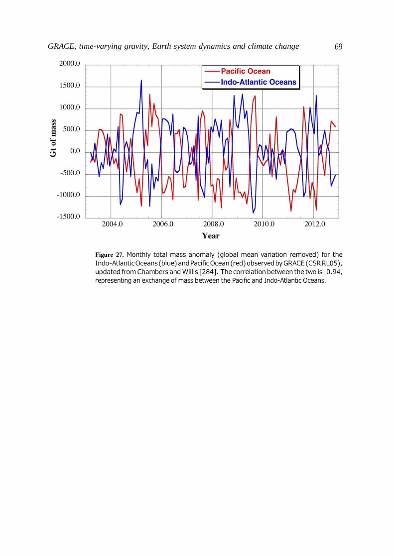
GRACE, time-varying gravity, Earth system dynamics and climate change 69
Figure 27. Monthly total mass anomaly (global mean variation removed) for the Indo-Atlantic Oceans (blue) and Pacific Ocean (red) observed by GRACE (CSR RL05), updated from Chambers and Willis [284]. The correlation between the two is -0.94, representing an exchange of mass between the Pacific and Indo-Atlantic Oceans.

REFERENCES 70
1629 References
1630
1631
1632
1633
1634
1635
1636
1637
1638
1639
1640
1641
1642
1643
1644
1645
1646
1647
1648
1649
1650
1651
1652
1653
1654
1655
1656
1657
1658
1659
1660
1661
1662
1663
1664
1665
1666
[1] D. Crossley, J. Hinderer, and U. Riccardi. The measurement of surface gravity. Reports on Progress in Physics, 76(4):046101, 2013.
[2] LAGEOS-I (Laser Geodynamics Satellite-I)/LAGEOS-II. URL https:// directory.eoportal.org/web/eoportal/satellite-missions/l/lageos.
[3] M. K. Cheng, R. J. Eanes, C. K. Shum, B. E. Schutz, and B. D. Tapley. Temporal variations in low degree zonal harmonics from Starlette orbit analysis. Geophys. Res. Lett., 16:393–396, May 1989. doi: 10.1029/GL016i005p00393.
[4] C. Reigber, H. Luhr, and P. Schwintzer. CHAMP mission status. Adv. Spac. Res., 30:129–134, July 2002. doi: 10.1016/S0273-1177(02)00276-4.
[5] R. S. Nerem, C. Jekeli, and W. M. Kaula. Gravity field determination and characteristics: Retrospective and prospective. J. Geophys. Res., 100:15053– 15074, 1995. doi: 10.1029/94JB03257.
[6] NASA. Geophysical and Geodetic Requirements for Global Gravity Field Measurements, 1987-2000: Report of a Gravity Workshop, Colorado Springs, CO. NASA geodyn. Branch, Division of Earth Science and Applications, Washington, D.C., 1987.
[7] NRC. Applications of a Dedicated Gravitational Satellite Mission. National Academy Press, Washington, D.C., 1979.
[8] NRC. A Strategy for Earth Science from Space in the 1980’s: Part I: Solid Earth and Oceans. National Academy Press, Washington, D.C., 1982.
[9] J. O. Dickey, C. R. Bentley, R. Bilham, J. A. Carton, R. J. Eanes, T. A. Herring, W. M. Kaula, G. S. E. Lagerloef, S. Rojstaczer, W. H. F. Smith, H. M. van den Dool, J. M. Wahr, and M. T. Zuber. Satellite Gravity and the Geosphere. National Research Council Report. National Academy Press, 1997.
[10] I. Ciufolini, A. Paolozzi, E. Pavlis, J. Ries, R. Koenig, R. Matzner, G. Sindoni, and H. Neumayer. Towards a one percent measurement of frame dragging by spin with satellite laser ranging to LAGEOS, LAGEOS 2 and LARES and grace gravity models. Space Science Reviews, 148(1-4):71–104, 2009. ISSN 0038-6308. doi: 10.1007/s11214-009-9585-7.
[11] R. R. B. von Frese, L. V. Potts, S. B. Wells, T. E. Leftwich, H. R. Kim, J. W. Kim, A. V. Golynsky, O. Hernandez, and L. R. Gaya-Pique. GRACE gravity evidence for an impact basin in Wilkes Land, Antarctica. Geochem. Geophy. Geosy., 10: 2014–+, February 2009. doi: 10.1029/2008GC002149.
[12] S. L. Bruinsma and J. M. Forbes. Storm-Time Equatorial Density Enhancements Observed by CHAMP and GRACE. J. Spacecraft Rockets, 44:1154–1159, November 2007. doi: 10.2514/1.28134.
[13] A. Cazenave and J. Chen. Time-variable gravity from space and present-day mass

REFERENCES 71
1667
1668
1669
1670
1671
1672
1673
1674
1675
1676
1677
1678
1679
1680
1681
1682
1683
1684
1685
1686
1687
1688
1689
1690
1691
1692
1693
1694
1695
1696
1697
1698
1699
1700
1701
1702
1703
1704
1705
redistribution in the Earth system. Earth and Planetary Science Letters, 298: 263–274, 10/2010 2010. doi: 10.1016/j.epsl.2010.07.035.
[14] V. Zlotnicki, S. Bettadpur, F. W. Landerer, and M. M. Watkins. Gravity Recovery and Climate Experiment (GRACE): Detection of Ice Mass Loss, Terrestrial Mass Changes, and Ocean Mass Gains Earth System Monitoring ed J. Orcutt (New York: Springer), pp. 123–152, 2013 doi: 10.1007/978-1-4614-5684-1 7.
[15] C. Reigber, R. Schmidt, F. Flechtner, R. K onig, U. Meyer, K.-H. Neumayer, P. Schwintzer, and S. Y. Zhu. An Earth gravity field model complete to degree and order 150 from GRACE: EIGEN-GRACE02S. J. geodyn., 39:1–10, January 2005. doi: 10.1016/j.jog.2004.07.001.
[16] B. Tapley, J. Ries, S. Bettadpur, D. Chambers, M. Cheng, F. Condi, B. Gunter, Z. Kang, P. Nagel, R. Pastor, T. Pekker, S. Poole, and F. Wang. GGM02 An improved Earth gravity field model from GRACE. J. Geodesy, 79:467–478, November 2005. doi: 10.1007/s00190-005-0480-z.
[17] S. V. Bettadpur. UTCSR level-2 processing standards document for level-2 product release 0004. Technical Report GRACE 327-742, CSR, Austin, TX, USA, 2007.
[18] F. Flechtner. GFZ level-2 processing standards document for level-2 product release 0004. Technical Report GRACE 327-743, GFZ, Potsdam, Germany, 2007.
[19] M. Watkins and D.-N. Yuan. JPL level-2 processing standards document for level-2 product release 04. Technical Report GRACE 327-744, JPL, Pasadena, CA, USA, 2007.
[20] J.-M. Lemoine, S. Bruinsma, S. Loyer, R. Biancale, J.-C. Marty, F. Perosanz, and G. Balmino. Temporal gravity field models inferred from GRACE data. Adv. Spac. Res., 39:1620–1629, 2007. doi: 10.1016/j.asr.2007.03.062.
[21] X. Liu. Global gravity field recovery from satellite-to-satellite tracking data with the acceleration approach. PhD. thesis, Netherlands Geodectic Commission, Publication on Geodesy 68, TU Delft, Delft, The Netherlands, 2008.
[22] T. Mayer-Gurr, A. Eicker, E. Kurtenbach, and K.-H. Ilk. ITG-GRACE: Global Static and Temporal Gravity Field Models from GRACE Data. In F. Flechtner, T. Gruber, A. Guntner, M. Mandea, M. Rothacher, T. Sch one, and J. Wickert, editors, System Earth via Geodetic-Geophysical Space Techniques, pages 159– 168. Springer, Berlin, Heidelberg, 2010. ISBN ISBN 978-3-642-10227-1. doi: 10.1007/978-3-642-10228-8 13.
[23] W. A. Heiskanen and H. Moritz. Physical geodesy. San Francisco, W. H. Freeman [1967], 1967.
[24] J. Wahr, M. Molenaar, and F. Bryan. Time variability of the earth’s gravity field: Hydrological and oceanic effects and their possible detection using GRACE. J. Geophys. Res. (Solid Earth), 103(B12):30305–30229, 1998.

REFERENCES 72
1706
1707
1708
1709
1710
1711
1712
1713
1714
1715
1716
1717
1718
1719
1720
1721
1722
1723
1724
1725
1726
1727
1728
1729
1730
1731
1732
1733
1734
1735
1736
1737
1738
1739
1740
1741
1742
1743
1744
[25] W. E. Farrell. Deformation of the Earth by surface loads. Rev. Geophys. and Space Phys., 10:761–797, August 1972.
[26] D. D. Rowlands, S. B. Luthcke, S. M. Klosko, F. G. R. Lemoine, D. S. Chinn, J. J. McCarthy, C. M. Cox, and O. B. Anderson. Resolving mass flux at high spatial and temporal resolution using GRACE intersatellite measurements. Geophys. Res. Lett., 32:4310–+, February 2005. doi: 10.1029/2004GL021908.
[27] S. B. Luthcke, H. J. Zwally, W. Abdalati, D. D. Rowlands, R. D. Ray, R. S. Nerem, F. G. Lemoine, J. J. McCarthy, and D. S. Chinn. Recent Greenland ice mass loss by drainage system from satellite gravity observations. Science, 314: 1286–1289, December 2006. doi: 10.1126/Science.1130776.
[28] B.D. Tapley, S. Bettadpur, J.C. Ries, P.F. Thompson, and M.M. Watkins. GRACE measurements of mass variability in the earth system. Science, 305, 2004.
[29] J. Wahr, S. Swenson, V. Zlotnicki, and I. Velicogna. Time variable gravity from GRACE: First results. Geophys. Res. Lett., 31:L11501, 2004. doi: 10.1029/ 2004GL019779.
[30] R. D. Ray and S. B. Luthcke. Tide model errors and GRACE gravimetry: towards a more realistic assessment. Geophys. J. Int., 167:1055–1059, December 2006. doi: 10.1111/j.1365-246X.2006.03229.x.
[31] E. J. O. Schrama and P. N. A. M. Visser. Accuracy assessment of the monthly GRACE geoids based upon a simulation. J. Geodesy, 81:67–80, January 2007. doi: 10.1007/s00190-006-0085-1.
[32] D. P. Chambers and J. A. Bonin. Evaluation of Release-05 GRACE time-variable gravity coefficients over the ocean. Ocean Science, 8:859–868, October 2012. doi: 10.5194/os-8-859-2012.
[33] S. Swenson and J. Wahr. Methods for inferring regional surface-mass anomalies from gravity recovery and climate experiment (GRACE) measurements of time- variable gravity. J. Geophys. Res., 107(B9):219, 2002. doi: 10.1029/2001JB000576.
[34] C. Jekeli. Alternative methods to smooth the Earth’s gravity field. Technical Report Report 327, Department of Geodetic Science and Surveying, Ohio State University, December 1981.
[35] J. L. Chen, C. R. Wilson, and K.-W. Seo. Optimized smoothing of Gravity Recovery and Climate Experiment (GRACE) time-variable gravity observations. J. Geophys. Res., 111:6408–+, June 2006. doi: 10.1029/2005JB004064.
[36] S.-C. Han, C. K. Shum, and K. Matsumoto. GRACE observations of M2 and S2
ocean tides underneath the Filchner-Ronne and Larsen ice shelves, Antarctica. Geophys. Res. Lett., 32:20311–+, October 2005. doi: 10.1029/2005GL024296.
[37] S. Swenson and J. Wahr. Post-processing removal of correlated errors in GRACE data. Geophys. Res. Lett., 33:L8402, April 2006. doi: 10.1029/2005GL025285.

REFERENCES 73
1745
1746
1747
1748
1749
1750
1751
1752
1753
1754
1755
1756
1757
1758
1759
1760
1761
1762
1763
1764
1765
1766
1767
1768
1769
1770
1771
1772
1773
1774
1775
1776
1777
1778
1779
1780
1781
1782
1783
[38] B. Wouters and E. J. O. Schrama. Improved accuracy of GRACE gravity solutions through empirical orthogonal function filtering of spherical harmonics. Geophys. Res. Lett., 34:23711–+, December 2007. doi: 10.1029/2007GL032098.
[39] J. Kusche. Approximate decorrelation and non-isotropic smoothing of time- variable GRACE-type gravity field models. J. Geodesy, pages 80–+, February 2007. doi: 10.1007/s00190-007-0143-3.
[40] R. Klees, E. A. Revtova, B. C. Gunter, P. Ditmar, E. Oudman, H. C. Winsemius, and H. H. G. Savenije. The design of an optimal filter for monthly GRACE gravity models. Geophys. J. Int., 175:417–432, November 2008. doi: 10.1111/j.1365-246X. 2008.03922.x.
[41] D. P. Chambers. Observing seasonal steric sea level variations with GRACE and satellite altimetry. J. Geophys. Res. (Oceans), 111:C3010, March 2006. doi: 10.1029/2005JC002914.
[42] J. L. Chen, C. R. Wilson, J. S. Famiglietti, and M. Rodell. Attenuation effect on seasonal basin-scale water storage changes from GRACE time-variable gravity. J. Geodesy, 81:237–245, April 2007. doi: 10.1007/s00190-006-0104-2.
[43] S. C. Swenson and J. M. Wahr. Estimating signal loss in regularized GRACE gravity field solutions. Geophys. J. Int., 185:693–702, May 2011. doi: 10.1111/j. 1365-246X.2011.04977.x.
[44] F. W. Landerer and S. C. Swenson. Accuracy of scaled GRACE terrestrial water storage estimates. Water Resour. Res. , 48:W04531, April 2012. doi: 10.1029/2011WR011453.
[45] H. Save, S. Bettadpur, and B. D. Tapley. Reducing errors in the GRACE gravity solutions using regularization. J. Geodesy, 86:695–711, September 2012. doi: 10.1007/s00190-012-0548-5.
[46] I. Velicogna and J. Wahr. Greenland mass balance from GRACE. Geophys. Res. Lett., 32:18505–+, September 2005. doi: 10.1029/2005GL023955.
[47] J. A. Bonin and D. P. Chambers. Evaluation of high-frequency oceanographic signal in GRACE data: Implications for de-aliasing. Geophys. Res. Lett., 381: L17608, September 2011. doi: 10.1029/2011GL048881.
[48] S. Bruinsma, J.-M. Lemoine, R. Biancale, and N. Vales. CNES/GRGS 10-day gravity field models (release 2) and their evaluation. Adv. Spac. Res., 45:587–601, February 2010. doi: 10.1016/j.asr.2009.10.012.
[49] F. Flechtner, C. Dahle, K. H. Neumayer, R. K onig, and C. F orste. The Release 04 CHAMP and GRACE EIGEN Gravity Field Models. In F. Flechtner, T. Gruber, A. Guntner, M. Mandea, M. Rothacher, T. Sch one, and J. Wickert, editors, System Earth via Geodetic-Geophysical Space Techniques, pages 41– 58. Springer, Berlin, Heidelberg, 2010. ISBN ISBN 978-3-642-10227-1. doi: 10.1007/978-3-642-10228-8 4.

REFERENCES 74
1784
1785
1786
1787
1788
1789
1790
1791
1792
1793
1794
1795
1796
1797
1798
1799
1800
1801
1802
1803
1804
1805
1806
1807
1808
1809
1810
1811
1812
1813
1814
1815
1816
1817
1818
1819
1820
1821
1822
1823
[50] E. Kurtenbach, T. Mayer-Gurr, and A. Eicker. Deriving daily snapshots of the Earth’s gravity field from GRACE L1B data using Kalman filtering. Geophys. Res. Lett., 36:17102–+, September 2009. doi: 10.1029/2009GL039564.
[51] T. H. Syed, J. S. Famiglietti, M. Rodell, J. Chen, and C. R. Wilson. Analysis of terrestrial water storage changes from GRACE and GLDAS. Water Resour. Res. , 44:2433–+, February 2008. doi: 10.1029/2006WR005779.
[52] R. Schmidt, P. Schwintzer, F. Flechtner, C. Reigber, A. Guntner, P. Doll, G. Ramillien, A. Cazenave, S. Petrovic, H. Jochmann, and J. Wunsch. GRACE observations of changes in continental water storage. Global Planet. Change, 50: 112–126, February 2006.
[53] K.-W. Seo, C. R. Wilson, J. S. Famiglietti, J. L. Chen, and M. Rodell. Terrestrial water mass load changes from Gravity Recovery and Climate Experiment (GRACE). Water Resour. Res. , 42:5417–+, May 2006. doi: 10.1029/ 2005WR004255.
[54] E. Rangelova, W. van der Wal, A. Braun, M. G. Sideris, and P. Wu. Analysis of Gravity Recovery and Climate Experiment time-variable mass redistribution signals over North America by means of principal component analysis. J. Geophys. Res. (Earth Surface), 112:3002–+, July 2007. doi: 10.1029/2006JF000615.
[55] R. Schmidt, S. Petrovic, A. Guntner, F. Barthelmes, J. Wunsch, and J. Kusche. Periodic components of water storage changes from GRACE and global hydrology models. J. Geophys. Res. (Solid Earth), 113:8419–+, August 2008. doi: 10.1029/ 2007JB005363.
[56] S. Swenson, P. J.-F. Yeh, J. Wahr, and J. Famiglietti. A comparison of terrestrial water storage variations from GRACE with in situ measurements from Illinois. Geophys. Res. Lett., 33:16401–+, August 2006. doi: 10.1029/2006GL026962.
[57] B. Creutzfeldt, A. Guntner, H. Thoss, B. Merz, and H. Wziontek. Measuring the effect of local water storage changes on in situ gravity observations: Case study of the Geodetic Observatory Wettzell, Germany. Water Resources Research, 46 W08531, 2010. doi: 10.1029/2009WR008359.
[58] M. Rodell, P. R. Houser, U. Jambor, J. Gottschalck, K. Mitchell, C.-J. Meng, K. Arsenault, B. Cosgrove, J. Radakovich, M. Bosilovich, J. K. Entin, J. P. Walker, D. Lohmann, and D. Toll. The Global Land Data Assimilation System. Bulletin of the American Meteorological Society, 85:381–394, March 2004. doi: 10.1175/BAMS-85-3-381.
[59] M. Rodell, J. Chen, H. Kato, J. S. Famiglietti, J. Nigro, and C. R. Wilson. Estimating groundwater storage changes in the Mississippi River basin (USA) using GRACE. Hydrogeology Journal, 15:159–166, February 2007. doi: 10.1007/ s10040-006-0103-7.
[60] S. Swenson, J. Famiglietti, J. Basara, and J. Wahr. Estimating profile soil moisture and groundwater variations using GRACE and Oklahoma Mesonet

REFERENCES 75
1824
1825
1826
1827
1828
1829
1830
1831
1832
1833
1834
1835
1836
1837
1838
1839
1840
1841
1842
1843
1844
1845
1846
1847
1848
1849
1850
1851
1852
1853
1854
1855
1856
1857
1858
1859
1860
1861
1862
soil moisture data. Water Resour. Res. , 44:1413–+, January 2008. doi: 10.1029/2007WR006057.
[61] G. Strassberg, B. R. Scanlon, and M. Rodell. Comparison of seasonal terrestrial water storage variations from GRACE with groundwater-level measurements from the High Plains Aquifer (USA). Geophys. Res. Lett., 34:14402–+, July 2007. doi: 10.1029/2007GL030139.
[62] J. L. Chen, C. R. Wilson, and B. D. Tapley. The 2009 exceptional Amazon flood and interannual terrestrial water storage change observed by GRACE. Water Resour. Res. , 46:12526–+, December 2010. doi: 10.1029/2010WR009383.
[63] H. Wang, L. Jia, H. Steffen, P. Wu, L. Jiang, H. Hsu, L. Xiang, Z. Wang, and B. Hu. Increased water storage in North America and Scandinavia from GRACE gravity data. Nature Geosci., 6:38–42, January 2013. doi: 10.1038/ngeo1652.
[64] M.-H. Lo, J. S. Famiglietti, P. J.-F. Yeh, and T. H. Syed. Improving parameter estimation and water table depth simulation in a land surface model using GRACE water storage and estimated base flow data. Water Resour. Res. , 46:5517–+, May 2010. doi: 10.1029/2009WR007855.
[65] S. Werth and A. Guntner. Calibration analysis for water storage variability of the global hydrological model WGHM. Hydrol. Earth. Syst. Sc. , 14:59–78, January 2010.
[66] B. Li, M. Rodell, B. F. Zaitchik, R. H. Reichle, R. D. Koster, and T. M. van Dam. Assimilation of GRACE terrestrial water storage into a land surface model: Evaluation and potential value for drought monitoring in western and central Europe. J. Hydrology, 446:103–115, June 2012. doi: 10.1016/j.jhydrol.2012.04.035.
[67] B. F. Zaitchik, M. Rodell, and R. H. Reichle. Assimilation of GRACE terrestrial water storage data into a land surface model: results for the Mississippi River Basin. J. Hydrometeorology, 9:535–548, June 2008. doi: 10.1175/2007JHM951.1.
[68] G.-Y. Niu and Z.-L. Yang. Assessing a land surface model’s improvements with GRACE estimates. Geophys. Res. Lett., 33:7401–+, April 2006. doi: 10.1029/2005GL025555.
[69] G.-Y. Niu, K.-W. Seo, Z.-L. Yang, C. Wilson, H. Su, J. Chen, and M. Rodell. Retrieving snow mass from GRACE terrestrial water storage change with a land surface model. Geophys. Res. Lett., 34:15704–+, August 2007. doi: 10.1029/2007GL030413.
[70] R. Houborg, M. Rodell, B. Li, R. Reichle, and B. F. Zaitchik. Drought indicators based on model-assimilated Gravity Recovery and Climate Experiment (GRACE) terrestrial water storage observations. Water Resour. Res. , 48:W07525, July 2012. doi: 10.1029/2011WR011291.
[71] A. Guntner. Improvement of global hydrological models using GRACE data. Surveys in Geophysics, 29(4-5):375–397, 2008. doi: 10.1007/s10712-008-9038-y.

REFERENCES 76
1863
1864
1865
1866
1867
1868
1869
1870
1871
1872
1873
1874
1875
1876
1877
1878
1879
1880
1881
1882
1883
1884
1885
1886
1887
1888
1889
1890
1891
1892
1893
1894
1895
1896
1897
1898
1899
1900
1901
1902
[72] P. D oll, H. Hoffmann-Dobrev, F. T. Portmann, S. Siebert, A. Eicker, M. Rodell, G. Strassberg, and B. R. Scanlon. Impact of water withdrawals from groundwater and surface water on continental water storage variations. J. geodyn., 59:143–156, September 2012. doi: 10.1016/j.jog.2011.05.001.
[73] H. Gao, Q. Tang, C. Ferguson, E. Wood, and D. Lettenmaier. Estimating the water budget of major US river basins via remote sensing. Int. J. Remote Sens., 31:3955–3978, April 2010. doi: 10.1080/01431161.2010.483488.
[74] J. Huang, J. Halpenny, W. van der Wal, C. Klatt, T. S. James, and A. Rivera. Detectability of groundwater storage change within the Great Lakes Water Basin using GRACE. J. Geophys. Res. (Solid Earth), 117:8401, 2012. doi: 10.1029/2011JB008876.
[75] S. Z. Yirdaw, K. R. Snelgrove, and C. O. Agboma. GRACE satellite observations of terrestrial moisture changes for drought characterization in the Canadian Prairie. J. Hydrology, 356:84–92, July 2008.
[76] D. Alsdorf, S.-C. Han, P. Bates, and J. Melack. Seasonal water storage on the amazon floodplain measured from satellites. Remote Sens. Environ. , 114(11): 2448 – 2456, 2010. ISSN 0034-4257. doi: 10.1016/j.rse.2010.05.020.
[77] J. L. Chen, C. R. Wilson, B. D. Tapley, L. Longuevergne, Z. L. Yang, and B. R. Scanlon. Recent La Plata basin drought conditions observed by satellite gravimetry. J. Geophys. Res. (Atmospheres), 115:22108–+, November 2010. doi: 10.1029/2010JD014689.
[78] F. Frappart, F. Papa, A. Guntner, S. Werth, J. Santos da Silva, J. Tomasella, F. Seyler, C. Prigent, W. B. Rossow, S. Calmant, and M.-P. Bonnet. Satellite- based estimates of groundwater storage variations in large drainage basins with extensive floodplains. Remote Sens. Environ. , 115(6):1588–1594, 2011. doi: 10.1016/j.rse.2011.02.003.
[79] A. Pereira and M. C. Pacino. Annual and seasonal water storage changes detected from GRACE data in the La Plata Basin. Phys. Earth Planet. In. , 212:88–99, December 2012. doi: 10.1016/j.pepi.2012.09.005.
[80] M. Ahmed, M. Sultan, J. Wahr, E. Yan, A. Milewski, W. Sauck, R. Becker, and B. Welton. Integration of GRACE (Gravity Recovery and Climate Experiment) data with traditional data sets for a better understanding of the time-dependent water partitioning in African watersheds. Geology, pages 479–482, 2011. doi: 10.1130/G31812.1.
[81] M. Becker, W. LLovel, A. Cazenave, A. Guntner, and J.-F. Cretaux. Recent hydrological behavior of the East African great lakes region inferred from GRACE, satellite altimetry and rainfall observations. Comptes Rendus Geoscience, 342: 223–233, March 2010.
[82] J. W. Crowley, J. X. Mitrovica, R. C. Bailey, M. E. Tamisiea, and J. L. Davis. Land water storage within the Congo Basin inferred from GRACE

REFERENCES 77
1903
1904
1905
1906
1907
1908
1909
1910
1911
1912
1913
1914
1915
1916
1917
1918
1919
1920
1921
1922
1923
1924
1925
1926
1927
1928
1929
1930
1931
1932
1933
1934
1935
1936
1937
1938
1939
1940
1941
satellite gravity data. Geophys. Res. Lett., 33:19402–+, October 2006. doi: 10.1029/2006GL027070.
[83] Hyongki Lee, R. Edward Beighley, Douglas Alsdorf, Hahn Chul Jung, C.K. Shum, Jianbin Duan, Junyi Guo, Dai Yamazaki, and Konstantinos Andreadis. Characterization of terrestrial water dynamics in the congo basin using {GRACE}
and satellite radar altimetry. Remote Sens. Environ. , 115(12):3530 – 3538, 2011. ISSN 0034-4257. doi: 10.1016/j.rse.2011.08.015.
[84] H. C. Winsemius, H. H. G. Savenije, N. C. van de Giesen, B. J. J. M. van den Hurk, E. A. Zapreeva, and R. Klees. Assessment of Gravity Recovery and Climate Experiment (GRACE) temporal signature over the upper Zambezi. Water Resour. Res. , 42:12201–+, December 2006. doi: 10.1029/2006WR005192.
[85] F. Seitz, M. Schmidt, and C. K. Shum. Signals of extreme weather conditions in Central Europe in GRACE 4-D hydrological mass variations. Earth Planet. Sc. Lett. , 268:165–170, April 2008. doi: 10.1016/j.epsl.2008.01.001.
[86] E. Forootan and J. Kusche. Separation of global time-variable gravity signals into maximally independent components. J. Geodesy, 86:477–497, July 2012. doi: 10.1007/s00190-011-0532-5.
[87] M. J. Leblanc, P. Tregoning, G. Ramillien, S. O. Tweed, and A. Fakes. Basin- scale, integrated observations of the early 21st century multiyear drought in southeast Australia. Water Resour. Res. , 45:4408–+, April 2009. doi: 10.1029/ 2008WR007333.
[88] D. Rieser, M. Kuhn, R. Pail, I. M. Anjasmara, and J. Awange. Relation between GRACE-derived surface mass variations and precipitation over Australia. Aust. J. Earth Sci., 57:887–900, October 2010. doi: 10.1080/08120099.2010.512645.
[89] O. Andersen, P. Berry, J. Freeman, F. G. Lemoine, S. Luthcke, K. Jakobsen, and M. Butts. Satellite Altimetry and GRACE Gravimetry for Studies of Annual Water Storage Variations in Bangladesh. Terr. Atmos. Ocean Sci., 19:47–52, 2008. doi: 10.3319/TAO.2008.19.1-2.47(SA).
[90] J. P. Moiwo, Y. Yang, F. Tao, W. Lu, and S. Han. Water storage change in the Himalayas from the Gravity Recovery and Climate Experiment (GRACE) and an empirical climate model. Water Resour. Res. , 470:W07521, July 2011. doi: 10.1029/2010WR010157.
[91] M. Rodell, I. Velicogna, and J. S. Famiglietti. Satellite-based estimates of groundwater depletion in India. Nature, 460:999–1002, August 2009. doi: 10.1038/nature08238.
[92] V. M. Tiwari, J. Wahr, and S. Swenson. Dwindling groundwater resources in northern India, from satellite gravity observations. Geophys. Res. Lett., 36:18401– +, September 2009. doi: 10.1029/2009GL039401.
[93] K. Yamamoto, Y. Fukuda, T. Nakaegawa, and J. Nishijima. Landwater variation

REFERENCES 78
1942
1943
1944
1945
1946
1947
1948
1949
1950
1951
1952
1953
1954
1955
1956
1957
1958
1959
1960
1961
1962
1963
1964
1965
1966
1967
1968
1969
1970
1971
1972
1973
1974
1975
1976
1977
1978
1979
1980
in four major river basins of the Indochina peninsula as revealed by GRACE. Earth Planets Space, 59:193–200, 2007.
[94] F. Frappart, G. Ramillien, and J. Famiglietti. Water balance of the Arctic drainage system using GRACE gravimetry products. Int. J. Remote Sens., 32:431–453, January 2011. doi: 10.1080/01431160903474954.
[95] F. W. Landerer, J. O. Dickey, and A. Guntner. Terrestrial water budget of the Eurasian pan-Arctic from GRACE satellite measurements during 2003– 2009. J. Geophys. Res. (Atmospheres), 115:23115–+, December 2010. doi: 10.1029/2010JD014584.
[96] David Garcıa-Garcıa, Caroline C. Ummenhofer, and Victor Zlotnicki. Australian water mass variations from grace data linked to indo-pacific climate variability. Remote Sens. Environ. , 115(9):2175 – 2183, 2011. ISSN 0034-4257. doi: 10.1016/j.rse.2011.04.007.
[97] W. Llovel, M. Becker, A. Cazenave, J.-F. Cretaux, and G. Ramillien. Global land water storage change from GRACE over 2002-2009; Inference on sea level. Comptes Rendus Geoscience, 342:179–188, March 2010.
[98] Y. Morishita and K. Heki. Characteristic precipitation patterns of El Nino/La Nina in time-variable gravity fields by GRACE. Earth Planet. Sc. Lett. , 272: 677–682, August 2008. doi: 10.1016/j.epsl.2008.06.003.
[99] T. Phillips, R. S. Nerem, B. Fox-Kemper, J. S. Famiglietti, and B. Rajagopalan. The influence of ENSO on global terrestrial water storage using GRACE. Geophys. Res. Lett., 39:L16705, August 2012. doi: 10.1029/2012GL052495.
[100] T. van Dam, J. Wahr, and D. Lavallee. A comparison of annual vertical crustal displacements from GPS and Gravity Recovery and Climate Experiment (GRACE) over Europe. J. Geophys. Res. (Solid Earth), 1112:B03404, March 2007. doi: 10.1029/2006JB004335.
[101] M. S. Steckler, S. L. Nooner, S. H. Akhter, S. K. Chowdhury, S. Bettadpur, L. Seeber, and M. G. Kogan. Modeling Earth deformation from monsoonal flooding in Bangladesh using hydrographic, GPS, and Gravity Recovery and Climate Experiment (GRACE) data. J. Geophys. Res. (Solid Earth), 115:8407–+, August 2010. doi: 10.1029/2009JB007018.
[102] J. Kusche and E. J. O. Schrama. Surface mass redistribution inversion from global GPS deformation and Gravity Recovery and Climate Experiment (GRACE) gravity data. J. Geophys. Res. (Solid Earth), 110:9409–+, September 2005. doi: 10.1029/2004JB003556.
[103] P. Tregoning, C. Watson, G. Ramillien, H. McQueen, and J. Zhang. Detecting hydrologic deformation using GRACE and GPS. Geophys. Res. Lett., 36:15401, August 2009. doi: 10.1029/2009GL038718.
[104] V. Tesmer, P. Steigenberger, T. van Dam, and T. Mayer-Gurr. Vertical

REFERENCES 79
1981
1982
1983
1984
1985
1986
1987
1988
1989
1990
1991
1992
1993
1994
1995
1996
1997
1998
1999
2000
2001
2002
2003
2004
2005
2006
2007
2008
2009
2010
2011
2012
2013
2014
2015
2016
2017
2018
2019
deformations from homogeneously processed GRACE and global GPS long-term series. J. Geodesy, 85:291–310, May 2011. doi: 10.1007/s00190-010-0437-8.
[105] P. Valty, O. de Viron, I. Panet, M. Van Camp, and J. Legrand. Assessing the precision in loading estimates by geodetic techniques in Southern Europe Geophysical Journal International, 194:1441–1454, 2013. doi: 10.1093/gji/ggt173.
[106] P. Doll, K. Fiedler, and J. Zhang. Global-scale analysis of river flow alterations due to water withdrawals and reservoirs. Hydrol. Earth. Syst. Sc. Discuss., 6: 4773–4812, July 2009.
[107] P. Doll and K. Fiedler. Global-scale modeling of groundwater recharge. Hydrol. Earth. Syst. Sc. , 12:863–885, May 2008.
[108] I. Haddeland, T. Skaugen, and D. P. Lettenmaier. Anthropogenic impacts on continental surface water fluxes. Geophys. Res. Lett., 33:L08406, April 2006. doi: 10.1029/2006GL026047.
[109] Y. Wada, L. P. H. van Beek, C. M. van Kempen, J. W. T. M. Reckman, S. Vasak, and M. F. P. Bierkens. Global depletion of groundwater resources. Geophys. Res. Lett., 37:L20402, October 2010. doi: 10.1029/2010GL044571.
[110] T. Jacob, J. Wahr, W. T. Pfeffer, and S. Swenson. Recent contributions of glaciers and ice caps to sea level rise. Nature, 482:514–518, February 2012. doi: 10.1038/nature10847.
[111] J. S. Famiglietti, M. Lo, S. L. Ho, J. Bethune, K. J. Anderson, T. H. Syed, S. C. Swenson, C. R. de Linage, and M. Rodell. Satellites measure recent rates of groundwater depletion in California’s Central Valley. Geophys. Res. Lett., 38: 3403–+, February 2011. doi: 10.1029/2010GL046442.
[112] A.L. Berger. Support for the astronomical theory of climatic change. Nature, 269 (5623):44–45, 1977.
[113] G. H. Roe and M. R. Allen. A comparison of competing explanations for the 100,000-yr ice age cycle. Geophys. Res. Lett., 26:2259–2262, 1999.
[114] Didier Paillard. Glacial cycles: Toward a new paradigm. Rev. Geophys.2, 39(3): 325–346, 2001. ISSN 1944-9208. doi: 10.1029/2000RG000091.
[115] A. Celsius. Anmarkningar om vatnets f orminskande sa i ostersj on som vesterhafvet. Kungl. Vet. Akad. Handl., pages 33–50, 1743.
[116] Charles Lyell. The bakerian lecture: On the proofs of a gradual rising of the land in certain parts of sweden. Philos. T. Roy. Soc., 125:pp. 1–38, 1835. ISSN 02610523.
[117] W. E. Farrell and J. A. Clark. On postglacial sea level. 46:647–667, 1976. [118] R.S. Woodward. On the form of and position of mean sea level. US Geol. Surv.
Bull., 48:87–170, 1888. [119] Roblyn A. Kendall, Konstantin Latychev, Jerry X. Mitrovica, Jonathan E.
Davis, and Mark E. Tamisiea. Decontaminating tide gauge records for the

REFERENCES 80
2020
2021
2022
2023
2024
2025
2026
2027
2028
2029
2030
2031
2032
2033
2034
2035
2036
2037
2038
2039
2040
2041
2042
2043
2044
2045
2046
2047
2048
2049
2050
2051
2052
2053
2054
2055
2056
2057
2058
2059
influence of glacial isostatic adjustment: The potential impact of 3-D Earth structure. Geophys. Res. Lett., 33(24), DEC 30 2006. ISSN 0094-8276. doi: 10.1029/2006GL028448.
[120] G. Spada, V. R. Barletta, V. Klemann, R. E. M. Riva, Z. Martinec, P. Gasperini, B. Lund, D. Wolf, L. L. A. Vermeersen, and M. A. King. A benchmark study for glacial isostatic adjustment codes. Geophys. J. Int., 185(1):106–132, APR 2011. ISSN 0956-540X. doi: 10.1111/j.1365-246X.2011.04952.x.
[121] A. M. Dziewonski and D. L. Anderson. Preliminary Reference Earth Model. Phys. Earth Planet. Inter., 25:297–356, 1981.
[122] Holger Steffen and Patrick Wu. Glacial isostatic adjustment in Fennoscandia-A review of data and modeling. J. Geodyn., 52(3-4):169–204, OCT 2011. ISSN 0264-3707. doi: 10.1016/j.jog.2011.03.002.
[123] N. A. Haskell. The motion of a viscous fluid under a surface load. Physics, 6: 265–369, 1935.
[124] W. R. Peltier. The impulse response of a Maxwell earth. Rev. Geophys. Space Phys., 12:649–669, 1974.
[125] L. M. Cathles. The Viscosity of the Earth’s Mantle. Princeton University Press, Princeton, 1975.
[126] Patrick Wu and W. R. Peltier. Viscous gravitational relaxation. 70:435–485, 1982. [127] K. Lambeck, P. Johnston, and M. Nakada. Holocene glacial rebound and sea level
change in NW Europe. Geophys. J. Int. 103:451–468, 1990. [128] J. X. Mitrovica and W. R. Peltier. Constraints on mantle viscosity from relative
sea level variations in Hudson Bay. Geophys. Res. Lett., 19:1185–1188, 1992. [129] L. L. A. Vermeersen, R. Sabadini, and G. Spada. Analytical visco-elastic relaxation
models. Geophys. Res. Lett., 23:697–700, 1996. [130] Glenn A. Milne and Jerry X. Mitrovica. Postglacial sea-level change on a rotating
earth. Geophys. J. Int. 133:1–19, 1998. [131] J. Hagedoorn, D. Wolf, and Z. Martinec. An estimate of global sea level rise
inferred from tide-gauge measurements using glacial-isostatic adjustment models consistent with the relative sea level record. Pure Appl. Geophys., 164(4):791–818, 2007.
[132] J. O. Dickey, S. L Marcus, O. de Viron, and I. Fukumori. Recent Earth oblateness variations: Unraveling climate and postglacial rebound effects. Science, 298(5600): 1975–1977, 2002.
[133] JX. Mitrovica, J. Wahr, I. Matsuyama, and A. Paulson. The rotational stability of an ice-age earth. Geophys. J. Int., 161:491–506, 2005.
[134] Z. Martinec and J. Hagedoorn. Time-domain approach to linearized rotational response of a three-dimensional viscoelastic earth model induced by glacial- isostatic adjustment: I. inertia-tensor perturbations. Geophys. J. Int., 163:443– 462, 2005.

REFERENCES 81
2060
2061
2062
2063
2064
2065
2066
2067
2068
2069
2070
2071
2072
2073
2074
2075
2076
2077
2078
2079
2080
2081
2082
2083
2084
2085
2086
2087
2088
2089
2090
2091
2092
2093
2094
2095
2096
2097
2098
2099
[135] R. Sabadini and L. L. A. Vermeersen. Long-term rotation instabilities of the Earth: A Reanalysis, volume 29. In: Ice Sheets, Sea Level and the Dynamic Earth, American Geophys. Union, 2002.
[136] Poalo Gasperini and Roberto Sabadini. Lateral heterogeneities on mantle viscosity and post-glacial rebound. Geophys. J. Int., 98:413–428, 1989.
[137] S. J. Zhong, A. Paulson, and J. Wahr. Three-dimensional finite-element modelling of earth’s viscoelastic deformation: effects of lateral variations in lithospheric thickness. Geophys. J. Int., 155:679–695, 2005.
[138] Jeroen Tromp and Jerry X. Mitrovica. Surface loading of a viscoelastic earth—II. spherical models. 137:856–872, 1999.
[139] Z. Martinec. Propagator-matrix technique for the viscoelastic response of a multi- layered sphere to surface toroidal traction. Pure Appl. Geophys., 164:663–681, 2007.
[140] Volker Klemann, Erik R. Ivins, Zdenek Martinec, and Detlef Wolf. Models of active glacial isostasy roofing warm subduction: Case of the South Patagonian Ice Field. J. GEOPHYSICAL RESEARCH-SOLID EARTH, 112(B9), SEP 25 2007. ISSN 0148-0227. doi: 10.1029/2006JB004818.
[141] Volker Klemann, Zdenek Martinec, and Erik R. Ivins. Glacial isostasy and plate motions. J. Geodyn., 46:95–103, 2008. doi: 10.1016/j.jog.2008.04.005.
[142] Geruo A, John Wahr, and Shijie Zhong. Computations of the viscoelastic response of a 3-d compressible earth to surface loading: an application to glacial isostatic adjustment in antarctica and canada. Geophys. J. Int., 2012. doi: 10.1093/gji/ggs030.
[143] C Giunchi and G. Spada. Postglacial rebound in a non-newtonian spherical earth. Geophys. Res. Lett., 27:2065–2068, 2000.
[144] W. van der Wal, P. Wu, H. Wang, and M.G. Sideris. ”sea levels and uplift rate from composite rheology in glacial isostatic adjustment modeling”. J. Geodyn., 50(1):38–48, 2010.
[145] Y. Tanaka, V. Klemann, Z. Martinec, and R. E. M. Riva. Spectral-finite element approach to viscoelastic relaxation in a spherical compressible Earth: application to GIA modelling. Geophys. J. Int., 184:220–234, 2011. doi: 10.1111/j.1365-246X. 2010.04854.x. pdf.
[146] Matt A. King, Rory J. Bingham, Phil Moore, Pippa L. Whitehouse, Michael J. Bentley, and Glenn A. Milne. Lower satellite-gravimetry estimates of Antarctic sea-level contribution. Nature, 491(7425):586–589, November 2012. doi: 10.1038/ nature11621.
[147] Andrew Shepherd, Erik R. Ivins, Geruo A, Valentina R. Barletta, Mike J. Bentley, Srinivas Bettadpur, Kate H. Briggs, David H. Bromwich, Rene Forsberg, Natalia Galin, Martin Horwath, Stan Jacobs, Ian Joughin, Matt A. King, Jan T. M. Lenaerts, Jilu Li, Stefan R. M. Ligtenberg, Adrian Luckman, Scott B. Luthcke,

REFERENCES 82
2100
2101
2102
2103
2104
2105
2106
2107
2108
2109
2110
2111
2112
2113
2114
2115
2116
2117
2118
2119
2120
2121
2122
2123
2124
2125
2126
2127
2128
2129
2130
2131
2132
2133
2134
2135
2136
2137
2138
Malcolm McMillan, Rakia Meister, Glenn Milne, Jeremie Mouginot, Alan Muir, Julien P. Nicolas, John Paden, Antony J. Payne, Hamish Pritchard, Eric Rignot, Helmut Rott, Louise Sandberg Sørensen, Ted A. Scambos, Bernd Scheuchl, Ernst J. O. Schrama, Ben Smith, Aud V. Sundal, Jan H. van Angelen, Willem J. van de Berg, Michiel R. van den Broeke, David G. Vaughan, Isabella Velicogna, John Wahr, Pippa L. Whitehouse, Duncan J. Wingham, Donghui Yi, Duncan Young, and H. Jay Zwally. A reconciled estimate of ice-sheet mass balance. Science, 338 (6111):1183–1189, 2012. doi: 10.1126/science.1228102.
[148] I. Velicogna and J. Wahr. Measurements of time-variable gravity show mass loss in Antarctica. Science, 311:1754–1756, March 2006. doi: 10.1126/Science.1123785.
[149] I. D. Thomas, M. A. King, M. J. Bentley, P. L. Whitehouse, N. T. Penna, S. D. P. Williams, R. E. M. Riva, D. A. Lavallee, P. J. Clarke, E. C. King, R. C. A. Hindmarsh, and H. Koivula. Widespread low rates of Antarctic glacial isostatic adjustment revealed by GPS observations. Geophys. Res. Lett., 38: L22302, November 2011. doi: 10.1029/2011GL049277.
[150] P. L. Whitehouse, M. J. Bentley, G. A. Milne, M. A. King, and I. D. Thomas. A new glacial isostatic adjustment model for Antarctica: calibrated and tested using observations of relative sea-level change and present-day uplift rates. Geophys. J. Int., 190:1464–1482, September 2012. doi: 10.1111/j.1365-246X.2012.05557.x.
[151] I. Sasgen, H. Konrad, E. R. Ivins, M. R. Van den Broeke, J. L. Bamber, Z. Martinec, and V. Klemann. Antarctic ice-mass balance 2003 to 2012: regional reanalysis of GRACE satellite gravimetry measurements with improved estimate of glacial-isostatic adjustment based on GPS uplift rates. The Cryosphere, 7(5): 1499–1512, 2013. doi: 10.5194/tc-7-1499-2013.
[152] W. R. Peltier. Global glacial isostasy and the surface of the ice-age earth: the ICE5G (VM2) model and GRACE. Ann. Rev. Earth Planet. Sci., 32:111–149, 2004.
[153] M. E. Tamisiea, J. X. Mitrovica, and J. L. Davis. GRACE gravity data constrain ancient ice geometries and continental dynamics over Laurentia. Science, 316 (5826):881–883, May 11 2007. ISSN 0036-8075. doi: 10.1126/science.1137157.
[154] W. van der Wal, P. Wu, M. G. Sideris, and C. K. Shum. Use of GRACE determined secular gravity rates for glacial isostatic adjustment studies in North-America. J. Geodyn., 46(3-5):144–154, 2008.
[155] I. Sasgen, V. Klemann, and Z. Martinec. Towards the inversion of GRACE gravity fields for present-day ice-mass changes and glacial-isostatic adjustment in North America and Greenland. Journal of Geodynamics, 59:49–63, 2012.
[156] J. Wahr, H. DaZhong, and A. Trupin. Predictions of vertical uplift caused by changing polar ice volumes on a viscoelastic Earth. Geophys. Res. Lett., 22(8): 977–980, 1995.

REFERENCES 83
2139
2140
2141
2142
2143
2144
2145
2146
2147
2148
2149
2150
2151
2152
2153
2154
2155
2156
2157
2158
2159
2160
2161
2162
2163
2164
2165
2166
2167
2168
2169
2170
2171
2172
2173
2174
2175
2176
2177
2178
[157] S. Mazzotti, A. Lambert, J. Henton, T. S. James, and N. Courtier. Absolute gravity calibration of GPS velocities and glacial isostatic adjustment in mid- continent North America. Geophys. Res. Lett., 38(24), 2011. doi: 10.1029/ 2011GL049846.
[158] Archie Paulson, Shijie Zhong, and John Wahr. Inference of mantle viscosity from GRACE and relative sea level data. Geophys. J. Int., 171(2):497–508, NOV 2007. ISSN 0956-540X. doi: 10.1111/j.1365-246X.2007.03556.x.
[159] J. L. Davis and members of BIFROST. GPS measurements to constrain geodynamic processes in Fennoscandia. EOS, 77:337–341, 1996.
[160] H. G. Scherneck, J. M. Johansson, H. Koivula, T. van Dam, and J. L. Davis. Vertical crustal motion observed in the BIFROST project. J. Geodyn., 35:425– 441, 2003.
[161] Holger Steffen, Patrick Wu, and Hansheng Wang. Determination of the Earth’s structure in Fennoscandia from GRACE and implications for the optimal post- processing of GRACE data. Geophys. J. Int., 182(3):1295–1310, SEP 2010. ISSN 0956-540X. doi: 10.1111/j.1365-246X.2010.04718.x.
[162] E. M. Hill, J. L. Davis, M. E. Tamisiea, and M. Lidberg. Combination of geodetic observations and models for glacial isostatic adjustment fields in fennoscandia. J. Geophys. Res., 115(B7):n/a–n/a, 2010. ISSN 2156-2202. doi: 10.1029/2009JB006967.
[163] V. Mikhailov, S. Tikhotsky, M. Diament, I. Panet, and V. Ballu. Can tectonic processes be recovered from new gravity satellite data? Earth and Planetary Science Letters, 228(34):281 – 297, 2004. doi: 10.1016/j.epsl.2004.09.035.
[164] O. De Viron, I. Panet, V. Mikhailov, M. Van Camp, and M. Diament. Retrieving earthquake signature in grace gravity solutions. Geophysical Journal International, 174(1):14–20+, 2008. doi: 10.1111/j.1365-246X.2008.03807.x.
[165] A. Nur and J. R. Booker. Aftershocks Caused by Pore Fluid Flow? Science, 175: 885–887, February 1972. doi: 10.1126/science.175.4024.885.
[166] G. Peltzer, P. Rosen, F. Rogez, and K. Hudnut. Poroelastic rebound along the Landers 1992 earthquake surface rupture. J. Geophys. Res., 103:30131, December 1998. doi: 10.1029/98JB02302.
[167] A. Nur and G. Mavko. Postseismic Viscoelastic Rebound. Science, 183:204–206, January 1974. doi: 10.1126/science.183.4121.204.
[168] Roland Burgmann and Georg Dresen. Rheology of the Lower Crust and Upper Mantle: Evidence from Rock Mechanics, Geodesy, and Field Observations. Annu. Rev. Earth Pl. Sc., 36(1):531–567, 2008. doi: 10.1146/annurev.earth.36.031207. 124326.
[169] S.-C. Han, C. K. Shum, M. Bevis, C. Ji, and C.-Y. Kuo. Crustal dilatation observed by GRACE after the 2004 Sumatra-Andaman earthquake. Science, 313: 658–662, August 2006. doi: 10.1126/science.1128661.

REFERENCES 84
2179
2180
2181
2182
2183
2184
2185
2186
2187
2188
2189
2190
2191
2192
2193
2194
2195
2196
2197
2198
2199
2200
2201
2202
2203
2204
2205
2206
2207
2208
2209
2210
2211
2212
2213
2214
2215
2216
2217
[170] Y. Okada. Surface Deformation Due to Shear and Tensile Faults in a Half-Space. Bull. Seis. Soc. Amer., 75(4):1135–1154, 1985.
[171] Fred F. Pollitz. Coseismic Deformation From Earthquake Faulting On A Layered Spherical Earth. Geophys. J. Int., 125(1):1–14, 1996. ISSN 1365-246X. doi: 10.1111/j.1365-246X.1996.tb06530.x.
[172] S.-C. Han, R. Riva, J. Sauber, and E. Okal. Source parameter inversion for recent great earthquakes from a decade-long observation of global gravity fields. J. Geophys. Res. (Solid Earth), 118(3):1240–1267, 2013. ISSN 2169-9356. doi: 10.1002/jgrb.50116.
[173] G. Cambiotti, A. Bordoni, R. Sabadini, and L. Colli. GRACE gravity data help constraining seismic models of the 2004 Sumatran earthquake. J. Geophys. Res. (Solid Earth), 116:B10403, October 2011. doi: 10.1029/2010JB007848.
[174] D. B. T. Broerse, L. L. A. Vermeersen, R. E. M. Riva, and W. van der Wal. Ocean contribution to co-seismic crustal deformation and geoid anomalies: Application to the 2004 December 26 Sumatra–Andaman earthquake. Earth Planet. Sc. Lett. , 305:341–349, May 2011. doi: 10.1016/j.epsl.2011.03.011.
[175] R. Ogawa and K. Heki. Slow postseismic recovery of geoid depression formed by the 2004 Sumatra-Andaman Earthquake by mantle water diffusion. Geophys. Res. Lett., 34:6313–+, March 2007. doi: 10.1029/2007GL029340.
[176] J. L. Chen, C. R. Wilson, B. D. Tapley, and S. Grand. GRACE detects coseismic and postseismic deformation from the Sumatra-Andaman earthquake. Geophys. Res. Lett., 34:13302–+, July 2007. doi: 10.1029/2007GL030356.
[177] I. Panet, V. Mikhailov, M. Diament, F. Pollitz, G. King, O. de Viron, M. Holschneider, R. Biancale, and J.-M. Lemoine. Coseismic and post-seismic signatures of the Sumatra 2004 December and 2005 March earthquakes in GRACE satellite gravity. Geophys. J. Int., 171:177–190, October 2007. doi: 10.1111/j.1365-246X.2007.03525.x.
[178] S.-C. Han, J. Sauber, and S. Luthcke. Regional gravity decrease after the 2010 Maule (Chile) earthquake indicates large-scale mass redistribution. Geophys. Res. Lett., 37:23307–+, December 2010. doi: 10.1029/2010GL045449.
[179] K. Heki and K. Matsuo. Coseismic gravity changes of the 2010 earthquake in central Chile from satellite gravimetry. Geophys. Res. Lett., 37:24306–+, December 2010. doi: 10.1029/2010GL045335.
[180] K. Matsuo and K. Heki. Coseismic gravity changes of the 2011 Tohoku-Oki earthquake from satellite gravimetry. Geophys. Res. Lett., 380:L00G12, September 2011. doi: 10.1029/2011GL049018.
[181] S.-C. Han, J. Sauber, and R. Riva. Contribution of satellite gravimetry to understanding seismic source processes of the 2011 Tohoku-Oki earthquake. Geophys. Res. Lett., 38:L24312, December 2011. doi: 10.1029/2011GL049975.

REFERENCES 85
2218
2219
2220
2221
2222
2223
2224
2225
2226
2227
2228
2229
2230
2231
2232
2233
2234
2235
2236
2237
2238
2239
2240
2241
2242
2243
2244
2245
2246
2247
2248
2249
2250
2251
2252
2253
2254
2255
2256
[182] R. S. Stein. The role of stress transfer in earthquake occurrence. Nature, 402: 605–609, December 1999. doi: 10.1038/45144.
[183] S.-C. Han and F. J. Simons. Spatiospectral localization of global geopotential fields from the Gravity Recovery and Climate Experiment (GRACE) reveals the coseismic gravity change owing to the 2004 Sumatra-Andaman earthquake. J. Geophys. Res. (Solid Earth), 113:1405–+, January 2008. doi: 10.1029/ 2007JB004927.
[184] X. Zhou, W. Sun, B. Zhao, G. Fu, J. Dong, and Z. Nie. Geodetic observations detecting coseismic displacements and gravity changes caused by the Mw = 9.0 Tohoku-Oki earthquake. J. Geophys. Res. (Solid Earth), 117:B05408, May 2012. doi: 10.1029/2011JB008849.
[185] G. Cambiotti and R. Sabadini. Gravitational seismology retrieving Centroid- Moment-Tensor solution of the 2011 Tohoku earthquake. J. Geophys. Res. (Solid Earth), 118:183–194, January 2013. doi: 10.1029/2012JB009555.
[186] L. Wang, C. K. Shum, F. J. Simons, A. Tassara, K. Erkan, C. Jekeli, A. Braun, C. Kuo, H. Lee, and D.-N. Yuan. Coseismic slip of the 2010 Mw 8.8 Great Maule, Chile, earthquake quantified by the inversion of GRACE observations. Earth Planet. Sc. Lett. , 335:167–179, June 2012. doi: 10.1016/j.epsl.2012.04.044.
[187] L. Wang, C. K. Shum, F. J. Simons, B. Tapley, and C. Dai. Coseismic and postseismic deformation of the 2011 Tohoku-Oki earthquake constrained by GRACE gravimetry. Geophys. Res. Lett., 39:L07301, April 2012. doi: 10.1029/2012GL051104.
[188] G. Cambiotti and R. Sabadini. A source model for the great 2011 Tohoku earthquake (Mw =9.1) from inversion of GRACE gravity data. Earth Planet. Sc. Lett. , 335:72–79, June 2012. doi: 10.1016/j.epsl.2012.05.002.
[189] V. C. Tsai, M. Nettles, G. Ekstr om, and A. M. Dziewonski. Multiple CMT source analysis of the 2004 Sumatra earthquake. Geophys. Res. Lett., 32:L17304, September 2005. doi: 10.1029/2005GL023813.
[190] E. A. Okal and S. Stein. Observations of ultra-long period normal modes from the 2004 Sumatra-Andaman earthquake. Phys. Earth Planet. In. , 175:53–62, June 2009. doi: 10.1016/j.pepi.2009.03.002.
[191] M. Hirschmann and D. Kohlstedt. Water in Earth’s mantle. Phys. Today, 65(3): 030000, 2012. doi: 10.1063/PT.3.1476.
[192] I. Panet, F. Pollitz, V. Mikhailov, M. Diament, P. Banerjee, and K. Grijalva. Upper mantle rheology from GRACE and GPS postseismic deformation after the 2004 Sumatra-Andaman earthquake. Geochem. Geophy. Geosy., 11:6008–+, June 2010. doi: 10.1029/2009GC002905.
[193] A. Hoechner, S. V. Sobolev, I. Einarsson, and R. Wang. Investigation on afterslip and steady state and transient rheology based on postseismic deformation and

REFERENCES 86
2257
2258
2259
2260
2261
2262
2263
2264
2265
2266
2267
2268
2269
2270
2271
2272
2273
2274
2275
2276
2277
2278
2279
2280
2281
2282
2283
2284
2285
2286
2287
2288
2289
2290
2291
2292
2293
2294
2295
geoid change caused by the Sumatra 2004 earthquake. Geochem. Geophy. Geosy., 12:Q07010, July 2011. doi: 10.1029/2010GC003450.
[194] F. F. Pollitz, R. Burgmann, and P. Banerjee. Post-seismic relaxation following the great 2004 Sumatra-Andaman earthquake on a compressible self-gravitating Earth. Geophys. J. Int., 167:397–420, October 2006. doi: 10.1111/j.1365-246X. 2006.03018.x.
[195] M. Hashimoto, N. Choosakul, M. Hashizume, S. Takemoto, H. Takiguchi, Y. Fukuda, and K. Fujimori. Crustal deformations associated with the great Sumatra-Andaman earthquake deduced from continuous GPS observation. Earth Planets Space, 58:127–139, February 2006.
[196] W. Thatcher. Nonlinear strain buildup and the earthquake cycle on the San Andreas Fault. J. Geophys. Res., 88:5893–5902, July 1983. doi: 10.1029/ JB088iB07p05893.
[197] M. van den Broeke, J. Bamber, J. Ettema, E. Rignot, E. Schrama, W.J. van de Berg, E. van Meijgaard, I. Velicogna, and B. Wouters. Partitioning Recent Greenland Mass Loss. Science, 326(5955):984–986, 2009. doi: 10.1126/science. 1178176.
[198] R. Thomas, C. Davis, E. Frederick, W. Krabill, Y. Li, S. Manizade, and C. Martin. A comparison of Greenland ice-sheet volume changes derived from altimetry measurements. J. Glaciol., 54(185):203–212, March 2008. ISSN 0022-1430. doi: 10.3189/002214308784886225.
[199] E. Rignot and P. Kanagaratnam. Changes in the velocity structure of the Greenland ice sheet. Science, 311:986–990, February 2006. doi: 10.1126/science. 1121381.
[200] Andrew Shepherd and Duncan Wingham. Recent Sea-Level Contributions of the Antarctic and Greenland Ice Sheets. Science, 315(5818):1529–1532, 2007. doi: 10.1126/science.1136776.
[201] I. Velicogna and J. Wahr. Acceleration of Greenland ice mass loss in spring 2004. Nature, 443:329–331, September 2006. doi: 10.1038/nature05168.
[202] B. Wouters, D. Chambers, and E.J.O. Schrama. GRACE observes small-scale mass loss in Greenland. Geophys. Res. Lett., 35:L20501, October 2008. doi: 10.1029/2008GL034816.
[203] Ingo Sasgen, Michiel van den Broeke, Jonathan L. Bamber, Eric Rignot, Louise S. Sørensen, Bert Wouters, Zdenek Martinec, Isabella Velicogna, and Sebastian B. Simonsen. Timing and origin of recent regional ice-mass loss in Greenland. Earth Planet. Sc. Lett. , 333-334:293–303, June 2012. ISSN 0012821X. doi: 10.1016/j.epsl.2012.03.033.
[204] Ch. Harig and F. J. Simons. Mapping Greenland’s mass loss in space and time. PNAS, 109:19934–19937, December 2012. doi: 10.1073/pnas.1206785109.

REFERENCES 87
2296
2297
2298
2299
2300
2301
2302
2303
2304
2305
2306
2307
2308
2309
2310
2311
2312
2313
2314
2315
2316
2317
2318
2319
2320
2321
2322
2323
2324
2325
2326
2327
2328
2329
2330
2331
2332
2333
2334
[205] J. Bonin and D. Chambers. Uncertainty estimates of a GRACE inversion modelling technique over Greenland using a simulation. Geophysical Journal International, 2013. doi: 10.1093/gji/ggt091.
[206] S. A. Khan, J. Wahr, M. Bevis, I. Velicogna, and E. Kendrick. Spread of ice mass loss into northwest Greenland observed by GRACE and GPS. Geophys. Res. Lett., 37:6501–+, March 2010. doi: 10.1029/2010GL042460.
[207] M. Tedesco, X. Fettweis, T. Mote, J. Wahr, P. Alexander, J. E. Box, and B. Wouters. Evidence and analysis of 2012 Greenland records from spaceborne observations, a regional climate model and reanalysis data. The Cryosphere, 7(2): 615–630, 2013. doi: 10.5194/tc-7-615-2013.
[208] J. L. Chen, C. R. Wilson, D. D. Blankenship, and B. D. Tapley. Antarctic mass rates from GRACE. Geophys. Res. Lett., 33:11502–+, June 2006. doi: 10.1029/2006GL026369.
[209] Brian Gunter, T. Urban, R. Riva, M. Helsen, R. Harpold, S. Poole, P. Nagel, B. Schutz, and B. Tapley. A comparison of coincident GRACE and ICESat data over Antarctica. J. Geodesy, 83(11):1051–1060, 2009. doi: 10.1007/ s00190-009-0323-4.
[210] M. Horwath, B. Legresy, F. Remy, F. Blarel, and J.-M. Lemoine. Consistent patterns of Antarctic ice sheet interannual variations from ENVISAT radar altimetry and GRACE satellite gravimetry. Geophys. J. Int., 189:863–876, May 2012. doi: 10.1111/j.1365-246X.2012.05401.x.
[211] J. L. Chen, C. R. Wilson, B. D. Tapley, and D. Blankenship. Antarctic regional ice loss rates from GRACE. Earth Planet. Sc. Lett. , 2007. doi: 10.1016/j.epsl.2007.10.057. in press.
[212] M. Horwath and R. Dietrich. Signal and error in mass change inferences from GRACE: the case of Antarctica. Geophys. J. Int., 177:849–864, June 2009. doi: 10.1111/j.1365-246X.2009.04139.x.
[213] I. Sasgen, H. Dobslaw, Z. Martinec, and M. Thomas. Satellite gravimetry observation of Antarctic snow accumulation related to ENSO. Earth and Planetary Science Letters, 299:352–358, 2010. doi: 10.1016/j.epsl.2010.09.015.
[214] J. L. Chen, C. R. Wilson, D. Blankenship, and B. D. Tapley. Accelerated Antarctic ice loss from satellite gravity measurements. Nature Geosci., 2:859–862, December 2009. doi: 10.1038/ngeo694.
[215] C. Boening, M. Lebsock, F. Landerer, and G. Stephens. Snowfall-driven mass change on the East Antarctic ice sheet. Geophys. Res. Lett., 39:L21501, November 2012. doi: 10.1029/2012GL053316.
[216] R. E. M. Riva, B. C. Gunter, T. J. Urban, B. L. A. Vermeersen, R. C. Lindenbergh, M. M. Helsen, J. L. Bamber, R. S. W. van de Wal, M. R. van den Broeke, and B. E. Schutz. Glacial Isostatic Adjustment over Antarctica from combined ICESat

REFERENCES 88
2335
2336
2337
2338
2339
2340
2341
2342
2343
2344
2345
2346
2347
2348
2349
2350
2351
2352
2353
2354
2355
2356
2357
2358
2359
2360
2361
2362
2363
2364
2365
2366
2367
2368
2369
2370
2371
2372
2373
2374
and GRACE satellite data. Earth Planet. Sc. Lett. , 288:516–523, November 2009. doi: 10.1016/j.epsl.2009.10.013.
[217] I. Velicogna and J. Wahr. A method for separating Antarctic postglacial rebound and ice mass balance using future ICESat Geoscience Laser Altimeter System, Gravity Recovery and Climate Experiment, and GPS satellite data. J. Geophys. Res. (Solid Earth), 107, October 2002. doi: 10.1029/2001JB000708.
[218] E. R. Ivins and T. S. James. Antarctic glacial isostatic adjustment: a new assessment. Antarct. Sci., 17(04):541–553, 2005. doi: 10.1017/ S0954102005002968.
[219] J. Ettema, M. R. van den Broeke, E. van Meijgaard, W. J. van de Berg, J. L. Bamber, J. E. Box, and R. C. Bales. Higher surface mass balance of the Greenland ice sheet revealed by high-resolution climate modeling. Geophys. Res. Lett., 36: L12501, June 2009. doi: 10.1029/2009GL038110.
[220] J. T. M. Lenaerts, M. R. van den Broeke, W. J. van de Berg, E. van Meijgaard, and P. Kuipers Munneke. A new, high-resolution surface mass balance map of Antarctica (1979-2010) based on regional atmospheric climate modeling. Geophys. Res. Lett., 39:L04501, February 2012. doi: 10.1029/2011GL050713.
[221] Andrew Shepherd, Erik R. Ivins, Geruo, Valentina R. Barletta, Mike J. Bentley, Srinivas Bettadpur, Kate H. Briggs, David H. Bromwich, Rene Forsberg, Natalia Galin, Martin Horwath, Stan Jacobs, Ian Joughin, Matt A. King, Jan T. M. Lenaerts, Jilu Li, Stefan R. M. Ligtenberg, Adrian Luckman, Scott B. Luthcke, Malcolm McMillan, Rakia Meister, Glenn Milne, Jeremie Mouginot, Alan Muir, Julien P. Nicolas, John Paden, Antony J. Payne, Hamish Pritchard, Eric Rignot, Helmut Rott, Louise S. Sørensen, Ted A. Scambos, Bernd Scheuchl, Ernst J. O. Schrama, Ben Smith, Aud V. Sundal, Jan H. van Angelen, Willem J. van de Berg, Michiel R. van den Broeke, David G. Vaughan, Isabella Velicogna, John Wahr, Pippa L. Whitehouse, Duncan J. Wingham, Donghui Yi, Duncan Young, and H. Jay Zwally. A Reconciled Estimate of Ice-Sheet Mass Balance. Science, 338 (6111):1183–1189, November 2012. ISSN 1095-9203. doi: 10.1126/science.1228102.
[222] B. Wouters, J. L. Bamber, M. R. van den Broeke, J. T. M. Lenaerts, and I. Sasgen. Limits in detecting acceleration of ice sheet mass loss due to climate variability. Nature Geoscience, 6:613–616, 2013. doi: 10.1038/ngeo1874.
[223] I. Velicogna. Increasing rates of ice mass loss from the Greenland and Antarctic ice sheets revealed by GRACE. Geophys. Res. Lett., 36:L19503, October 2009. doi: 10.1029/2009GL040222.
[224] E. Rignot, I. Velicogna, M. R. van den Broeke, A. Monaghan, and J. Lenaerts. Acceleration of the contribution of the Greenland and Antarctic ice sheets to sea level rise. Geophys. Res. Lett., 38:L05503, March 2011. doi: 10.1029/ 2011GL046583.
[225] P. L. Svendsen, O. B. Andersen, and A. A. Nielsen. Acceleration of the Greenland

REFERENCES 89
2375
2376
2377
2378
2379
2380
2381
2382
2383
2384
2385
2386
2387
2388
2389
2390
2391
2392
2393
2394
2395
2396
2397
2398
2399
2400
2401
2402
2403
2404
2405
2406
2407
2408
2409
2410
2411
2412
2413
ice sheet mass loss as observed by GRACE: Confidence and sensitivity. Earth and Planetary Science Letters, 364:24–29, 2013. doi: 10.1016/j.epsl.2012.12.010.
[226] Roger J. Braithwaite. After six decades of monitoring glacier mass balance we still need data but it should be richer data. Ann. Glaciol., 50(1):191–197. ISSN 0260-3055. doi: 10.3189/172756409787769573.
[227] Anthony A. Arendt, Keith A. Echelmeyer, William D. Harrison, Craig S. Lingle, and Virginia B. Valentine. Rapid Wastage of Alaska Glaciers and Their Contribution to Rising Sea Level. Science, 297(5580):382–386, 2002. doi: 10.1126/science.1072497.
[228] M. E. Tamisiea, E. W. Leuliette, J. L. Davis, and J. X. Mitrovica. Constraining hydrological and cryospheric mass flux in southeastern Alaska using space-based gravity measurements. Geophys. Res. Lett., 32:20501–+, October 2005. doi: 10.1029/2005GL023961.
[229] J. L. Chen, B. D. Tapley, and C. R. Wilson. Alaskan mountain glacial melting observed by satellite gravimetry. Earth Planet. Sc. Lett. , 248:368–378, August 2006. doi: 10.1016/j.epsl.2006.05.039.
[230] S. B. Luthcke, A. A. Arendt, D. D. Rowlands, J. J. McCarthy, and C. F. Larsen. Recent glacier mass changes in the Gulf of Alaska region from GRACE mascon solutions. J. Glaciol., 54:767–777, 2008. doi: 10.3189/002214308787779933.
[231] A. Arendt, S. Luthcke, A. Gardner, S. O’Neel, D. Hill, G. Moholdt, and W. Abdalati. Analysis of a GRACE global mascon solution for Gulf of Alaska glaciers. Journal of Glaciology, 59:913–924, 2013. doi: 10.3189/2013JoG12J197.
[232] Alex S. Gardner, Geir Moholdt, J. Graham Cogley, Bert Wouters, Anthony A. Arendt, John Wahr, Etienne Berthier, Regine Hock, W. Tad Pfeffer, Georg Kaser, Stefan R. M. Ligtenberg, Tobias Bolch, Martin J. Sharp, Jon Ove Hagen, Michiel R. van den Broeke, and Frank Paul. A Reconciled Estimate of Glacier Contributions to Sea Level Rise: 2003 to 2009. Science, 340(6134):852–857, 2013. doi: 10.1126/science.1234532.
[233] A. S. Gardner, G. Moholdt, B. Wouters, G. J. Wolken, D. O. Burgess, M. J. Sharp, J. G. Cogley, C. Braun, and C. Labine. Sharply increased mass loss from glaciers and ice caps in the Canadian Arctic Archipelago. Nature, 473:357–360, May 2011. doi: 10.1038/nature10089.
[234] A. S. Gardner, G. Moholdt, A. Arendt, and B. Wouters. Long-term contributions of Baffin and Bylot Island Glaciers to sea level rise: an integrated approach using airborne and satellite laser altimetry, stereoscopic imagery and satellite gravimetry. The Cryosphere Discuss., 6:1563–1610, April 2012. doi: 10.5194/ tcd-6-1563-2012.
[235] Jan T. M. Lenaerts, Jan H. van Angelen, Michiel R. van den Broeke, Alex S. Gardner, Bert Wouters, and Erik van Meijgaard. Irreversible mass loss of

REFERENCES 90
2414
2415
2416
2417
2418
2419
2420
2421
2422
2423
2424
2425
2426
2427
2428
2429
2430
2431
2432
2433
2434
2435
2436
2437
2438
2439
2440
2441
2442
2443
2444
2445
2446
2447
2448
2449
2450
2451
2452
Canadian Arctic Archipelago glaciers. Geophys. Res. Lett., 40(5):870–874, 2013. ISSN 1944-8007. doi: 10.1002/grl.50214.
[236] M. B. Dyurgerov. Reanalysis of Glacier Changes: From the IGY to the IPY, 1960-2008. Data of Glaciological Studies, 108:1–116, 2010.
[237] G. Moholdt, B. Wouters, and A. S. Gardner. Recent mass changes of glaciers in the Russian High Arctic. Geophys. Res. Lett., 39:L10502, May 2012. doi: 10.1029/2012GL051466.
[238] E. Rignot, A. Rivera, and G. Casassa. Contribution of the Patagonia icefields of South America to sea level rise. Science, 302:434–437, October 2003.
[239] J. L. Chen, C. R. Wilson, B. D. Tapley, D. D. Blankenship, and E. R. Ivins. Patagonia Icefield melting observed by Gravity Recovery and Climate Experiment (GRACE). Geophys. Res. Lett., 34:22501–+, November 2007. doi: 10.1029/2007GL031871.
[240] M. J. Willis, A. K. Melkonian, M. E. Pritchard, and A. Rivera. Ice loss from the Southern Patagonian Ice Field, South America, between 2000 and 2012. Geophys. Res. Lett., 39:L17501, September 2012. doi: 10.1029/2012GL053136.
[241] Erik R. Ivins, Michael M. Watkins, Dah-Ning Yuan, Reinhard Dietrich, Gino Casassa, and Axel Rulke. On-land ice loss and glacial isostatic adjustment at the Drake Passage: 2003–2009. J. Geophys. Res. (Solid Earth), 116(B2), 2011. ISSN 2156-2202. doi: 10.1029/2010JB007607.
[242] K. Matsuo and K. Heki. Time-variable ice loss in Asian high mountains from satellite gravimetry. Earth Planet. Sc. Lett. , 290:30–36, February 2010. doi: 10.1016/j.epsl.2009.11.053.
[243] C. Wunsch and E. M. Gaposchkin. On Using Satellite Altimetry to Determine the General Circulation of the Oceans With Application to Geoid Improvement (Paper 80R0631). Rev. Geophys. and Space Phys., 18:725, November 1980. doi: 10.1029/RG018i004p00725.
[244] D. Stammer and C. Wunsch. Preliminary assessment of the accuracy and precision of TOPEX/POSEIDON altimeter data with respect to the large-scale ocean circulation. J. Geophys. Res., 99:24584, December 1994. doi: 10.1029/94JC00919.
[245] B. D. Tapley, D. P. Chambers, C. K. Shum, R. J. Eanes, J. C. Ries, and R. H. Stewart. Accuracy assessment of the large-scale dynamic ocean topography from TOPEX/POSEIDON altimetry. J. Geophys. Res., 99:24605, December 1994. doi: 10.1029/94JC01827.
[246] F. G. Lemoine, S. C. Kenyon, J. K. Factor, R.G. Trimmer, N. K. Pavlis, D. S. Chinn, C. M. Cox, S. M. Klosko, S. B. Luthcke, M. H. Torrence, Y. M. Wang, R. G. Williamson, E. C. Pavlis, R. H. Rapp, and T. R. Olson. The Development of the Joint NASA GSFC and the NIMA Geopotential Model EGM96. NASA/TP- 1998-206861, July 1998.

REFERENCES 91
2453
2454
2455
2456
2457
2458
2459
2460
2461
2462
2463
2464
2465
2466
2467
2468
2469
2470
2471
2472
2473
2474
2475
2476
2477
2478
2479
2480
2481
2482
2483
2484
2485
2486
2487
2488
2489
2490
2491
[247] B. D. Tapley, D. P. Chambers, S. Bettadpur, and J. C. Ries. Large scale ocean circulation from the GRACE GGM01 Geoid. Geophys. Res. Lett., 30:2163, November 2003. doi: 10.1029/2003GL018622.
[248] R. J. Bingham, P. Knudsen, O. Andersen, and R. Pail. An initial estimate of the North Atlantic steady-state geostrophic circulation from GOCE. Geophys. Res. Lett., 38:L01606, January 2011. doi: 10.1029/2010GL045633.
[249] P. Knudsen, R. Bingham, O. Andersen, and M.-H. Rio. A global mean dynamic topography and ocean circulation estimation using a preliminary GOCE gravity model. J. Geodesy, 85:861–879, November 2011. doi: 10.1007/s00190-011-0485-8.
[250] N. K. Pavlis, S. A. Holmes, S. C. Kenyon, and J. K. Factor. The development and evaluation of the Earth Gravitational Model 2008 (EGM2008). J. Geophys. Res. (Solid Earth), 117:B04406, April 2012. doi: 10.1029/2011JB008916.
[251] T. Kanzow, F. Flechtner, A. Chave, R. Schmidt, P. Schwintzer, and U. Send. Seasonal variation of ocean bottom pressure derived from Gravity Recovery and Climate Experiment (GRACE): Local validation and global patterns. J. Geophys. Res. (Oceans), 110:C9001, September 2005. doi: 10.1029/2004JC002772.
[252] D.P. Chambers, J. Wahr, and R.S. Nerem. Preliminary observations of global ocean mass variations with GRACE. Geophys. Res. Lett., 31:L13310, 2004. doi: 10.1029/2004GL020461.
[253] R. M. Ponte. Oceanic Response to Surface Loading Effects Neglected in Volume- Conserving Models. J. Phys. Oceanogr., 36:426–434, June 2006. doi: 10.1175/ JPO2843.1.
[254] K. Lorbacher, S. J. Marsland, J. A. Church, S. M. Griffies, and D. Stammer. Rapid barotropic sea level rise from ice sheet melting. J. Geophys. Res. (Oceans), 117:C06003, June 2012. doi: 10.1029/2011JC007733.
[255] W. R. Peltier. Closure of the budget of global sea level rise over the GRACE era: the importance and magnitudes of the required corrections for global glacial isostatic adjustment. Quaternary Sci. Rev., 28:1658–1674, August 2009. doi: 10.1016/j.quascirev.2009.04.004.
[256] D. P. Chambers, J. Wahr, M. E. Tamisiea, and R. S. Nerem. Ocean mass from GRACE and glacial isostatic adjustment. J. Geophys. Res. (Solid Earth), 115: B11415, November 2010. doi: 10.1029/2010JB007530.
[257] W. R. Peltier, R. Drummond, and K. Roy. Comment on ”Ocean mass from GRACE and glacial isostatic adjustment” by D. P. Chambers et al. J. Geophys. Res. (Solid Earth), 117:B11403, November 2012. doi: 10.1029/2011JB008967.
[258] D. P. Chambers, J. Wahr, M. E. Tamisiea, and R. S. Nerem. Reply to comment by W. R. Peltier et al. on ”Ocean mass from GRACE and glacial isostatic adjustment”. J. Geophys. Res. (Solid Earth), 117:B11404, November 2012. doi: 10.1029/2012JB009441.

REFERENCES 92
2492
2493
2494
2495
2496
2497
2498
2499
2500
2501
2502
2503
2504
2505
2506
2507
2508
2509
2510
2511
2512
2513
2514
2515
2516
2517
2518
2519
2520
2521
2522
2523
2524
2525
2526
2527
2528
2529
2530
[259] J. L. Chen, C. R. Wilson, D. P. Chambers, R. S. Nerem, and B. D. Tapley. Seasonal global water mass budget and mean sea level variations. Geophys. Res. Lett., 25:3555–3558, 1998. doi: 10.1029/98GL02754.
[260] J.F. Minster, A. Cazenave, Y.V. Serafini, F. Mercier, M.C. Gennero, and P. Rogel. Annual cycle in mean sea level from topexposeidon and ers-1: inference on the global hydrological cycle. Global Planet. Change, 20(1):57 – 66, 1999. ISSN 0921- 8181. doi: 10.1016/S0921-8181(98)00058-7.
[261] J. K. Willis, D. P. Chambers, and R. S. Nerem. Assessing the globally averaged sea level budget on seasonal to interannual timescales. J. Geophys. Res., 2008. doi: 10.1029/2007JC004517. in press.
[262] A. Cazenave and R.S. Nerem. Present-day sea level change: obervations and causes. ROG, 42:RG3001, 2004.
[263] J. K. Willis, D. Roemmich, and B. Cornuelle. Interannual variability in upper ocean heat content, temperature, and thermosteric expansion on global scales. J. Geophys. Res. (Oceans), 109:C12036, December 2004. doi: 10.1029/ 2003JC002260.
[264] A. Lombard, D. Garcia, G. Ramillien, A. Cazenave, R. Biancale, J. M. Lemoine, F. Flechtner, R. Schmidt, and M. Ishii. Estimation of steric sea level variations from combined GRACE and Jason-1 data. Earth Planet. Sc. Lett. , 254:194–202, February 2007. doi: 10.1016/j.epsl.2006.11.035.
[265] E. W. Leuliette and L. Miller. Closing the sea level rise budget with altimetry, Argo, and GRACE. Geophys. Res. Lett., 36:4608–+, February 2009. doi: 10.1029/2008GL036010.
[266] A. Cazenave, K. Dominh, S. Guinehut, E. Berthier, W. Llovel, G. Ramillien, M. Ablain, and G. Larnicol. Sea level budget over 2003-2008: A reevaluation from GRACE space gravimetry, satellite altimetry and Argo. Global Planet. Change, 65:83–88, January 2009.
[267] R. S. Nerem, D. P. Chambers, C. Choe, and G. T. Mitchum. Estimating Mean Sea Level Change from the TOPEX and Jason Altimeter Missions. Marine Geodesy, 33(sup1):435–446, 2010. doi: 10.1080/01490419.2010.491031.
[268] J.K. Willis, D. P. Chambers, C.-Y. Kuo, and C. K. Shum. Global Sea Level Rise: Recent Progress and Challenges for the Decade to Come. Oceanography, 23:26–35, 2010. doi: 10.5670/oceanog.2010.03.
[269] E. W. Leuliette and J. K. Willis. Balancing the Sea Level Budget. Oceanography, 24:122–129, 2011. doi: 10.5670/oceanog.2011.32.
[270] C. Boening, J. K. Willis, F. W. Landerer, R. S. Nerem, and J. Fasullo. The 2011 La Nina: So strong, the oceans fell. Geophys. Res. Lett., 39:L19602, October 2012. doi: 10.1029/2012GL053055.
[271] J. T. Fasullo, C. Boening, F. W. Landerer, and R. S. Nerem. Australia’s unique

REFERENCES 93
2531
2532
2533
2534
2535
2536
2537
2538
2539
2540
2541
2542
2543
2544
2545
2546
2547
2548
2549
2550
2551
2552
2553
2554
2555
2556
2557
2558
2559
2560
2561
2562
2563
2564
2565
2566
2567
2568
influence on global sea level in 2010–2011. Geophys. Res. Lett., 40(16):4368–4373, 2013. doi: 10.1002/grl.50834.
[272] D. P. Chambers, J. Chen, R. S. Nerem, and B. D. Tapley. Interannual mean sea level change and the Earth’s water mass budget. Geophys. Res. Lett., 27: 3073–3076, 2000. doi: 10.1029/2000GL011595.
[273] T. Ngo-Duc, K. Laval, J. Polcher, A. Lombard, and A. Cazenave. Effects of land water storage on global mean sea level over the past half century. Geophys. Res. Lett., 32(9):n/a–n/a, 2005. ISSN 1944-8007. doi: 10.1029/2005GL022719.
[274] D. P. Chambers and J. Schr oter. Measuring ocean mass variability from satellite gravimetry. J. geodyn., 52:333–343, December 2011. doi: 10.1016/j.jog.2011.04. 004.
[275] J. Morison, J. Wahr, R. Kwok, and C. Peralta-Ferriz. Recent trends in Arctic Ocean mass distribution revealed by GRACE. Geophys. Res. Lett., 34:7602–+, April 2007. doi: 10.1029/2006GL029016.
[276] James Morison, Ron Kwok, Cecilia Peralta-Ferriz, Matt Alkire, Ignatius Rigor, Roger Andersen, and Mike Steele. Changing Arctic Ocean freshwater pathways. Nature, 481(7379):66–70, January 2012. doi: 10.1038/nature10705.
[277] R. M. Ponte. A preliminary model study of the large-scale seasonal cycle in bottom pressure over the global ocean. J. Geophys. Res., 104:1289–1300, 1999. doi: 10.1029/1998JC900028.
[278] R. J. Bingham and C. W. Hughes. Observing seasonal bottom pressure variability in the North Pacific with GRACE. Geophys. Res. Lett., 33:L8607, April 2006. doi: 10.1029/2005GL025489.
[279] Y. T. Song and V. Zlotnicki. Subpolar ocean bottom pressure oscillation and its links to the tropical enso. Int. J. Remote Sens., 29(21):6091–6107, 2008. doi: doi:10.1080/01431160802175538.
[280] D. P. Chambers and J. K. Willis. Analysis of large-scale ocean bottom pressure variability in the North Pacific. J. Geophys. Res. (Oceans), 113:11003–+, November 2008. doi: 10.1029/2008JC004930.
[281] D. P. Chambers. ENSO-correlated fluctuations in ocean bottom pressure and wind-stress curl in the North Pacific. Ocean Science, 7(5):685–692, 2011. doi: 10.5194/os-7-685-2011.
[282] D. Stammer, R. Tokmakian, A. Semtner, and C Wunsch. How well does a 1/4◦
global circulation model simulate large-scale oceanic observations? J. Geophys. Res., 101:25779, November 1996. doi: 10.1029/96JC01754.
[283] V. N. Stepanov and C. W. Hughes. Propagation of signals in basin-scale ocean bottom pressure from a barotropic model. J. Geophys. Res. (Oceans), 111:C12002, December 2006. doi: 10.1029/2005JC003450.

REFERENCES 94
2569
2570
2571
2572
2573
2574
2575
2576
2577
2578
2579
2580
2581
2582
2583
2584
[284] D. P. Chambers and J. K. Willis. Low-frequency exchange of mass between ocean basins. J. Geophys. Res. (Oceans), 114:11008–+, November 2009. doi: 10.1029/2009JC005518.
[285] S. A. Cunningham, S. G. Alderson, B. A. King, and M. A. Brandon. Transport and variability of the Antarctic Circumpolar Current in Drake Passage. J. Geophys. Res. (Oceans), 108:8084, May 2003. doi: 10.1029/2001JC001147.
[286] C. W. Hughes, P. L. Woodworth, M. P. Meredith, V. Stepanov, T. Whitworth, and A. R. Pyne. Coherence of Antarctic sea levels, Southern Hemisphere Annular Mode, and flow through Drake Passage. Geophys. Res. Lett., 30:1464, May 2003. doi: 10.1029/2003GL017240.
[287] J. C. Fyfe and O. A. Saenko. Simulated changes in the extratropical Southern Hemisphere winds and currents. Geophys. Res. Lett., 33:L06701, March 2006. doi: 10.1029/2005GL025332.
[288] V. Zlotnicki, J. Wahr, I. Fukumori, and Y. Song. Antarctic circumpolar current transport variability during 2003-05 from GRACE. J. Phys. Oceanogr., 37(2): 230–244, 2007.
2585 [289] C.
Bo ning, R. Timmermann, S. Danilov, and J. Schr oter. Antarctic circumpolar
2586
2587
2588
2589
2590
2591
2592
2593
2594
2595
2596
2597
2598
2599
2600
2601
2602
2603
2604
2605
2606
2607
current transport variability in grace gravity solutions and numerical ocean model simulations. In F. Flechtner, T. Gruber, A. Guntner, M. Mandea, M. Rothacher, T. Sch one, and J. Wickert, editors, System Earth via Geodetic-Geophysical Space Techniques, pages 187–199. Springer, Berlin, Heidelberg, 2010. ISBN ISBN 978- 3-642-10227-1. doi: 10.1007/978-3-642-10228-8 15.
[290] I. Bergmann and H. Dobslaw. Short-term transport variability of the Antarctic Circumpolar Current from satellite gravity observations. J. Geophys. Res. (Oceans), 117:C05044, May 2012. doi: 10.1029/2012JC007872.
[291] P. Tregoning, K. Lambeck, and G. Ramillien. GRACE estimates of sea surface height anomalies in the Gulf of Carpentaria, Australia. Earth Planet. Sc. Lett. , 271:241–244, July 2008. doi: 10.1016/j.epsl.2008.04.018.
[292] B. Wouters and D. Chambers. Analysis of seasonal ocean bottom pressure variability in the Gulf of Thailand from GRACE. Global Planet. Change, 74: 76–81, November 2010.
[293] R.E.M. Riva, J.L. Bamber, D. A. Lavalle, and B. Wouters. Sea-level fingerprint of continental water and ice mass change from GRACE. Geophys. Res. Lett., 37: L19605, 2010. doi: 10.1029/2010GL044770.
[294] N. T. Vinogradova, R. M. Ponte, M. E. Tamisiea, K. J. Quinn, E. M. Hill, and J. L. Davis. Self-attraction and loading effects on ocean mass redistribution at monthly and longer time scales. J. Geophys. Res. (Oceans), 116:C08041, August 2011. doi: 10.1029/2011JC007037.
[295] B. Wouters, R. E. M. Riva, D. A. Lavallee, and J. L. Bamber. Seasonal variations

REFERENCES 95
2608
2609
2610
2611
2612
2613
2614
2615
2616
2617
2618
2619
2620
2621
2622
2623
2624
2625
2626
2627
2628
2629
2630
2631
2632
2633
2634
2635
2636
2637
2638
2639
2640
2641
2642
2643
2644
2645
2646
in sea level induced by continental water mass: First results from GRACE. Geophys. Res. Lett., 38:3303–+, February 2011. doi: 10.1029/2010GL046128.
[296] B. Killett, J. Wahr, S. Desai, D. Yuan, and M. Watkins. Arctic Ocean tides from GRACE satellite accelerations. J. Geophys. Res. (Oceans), 116:C11005, November 2011. doi: 10.1029/2011JC007111.
[297] R. D. Ray, S. B. Luthcke, and J.-P. Boy. Qualitative comparisons of global ocean tide models by analysis of intersatellite ranging data. J. Geophys. Res. (Oceans), 114:9017–+, September 2009. doi: 10.1029/2009JC005362.
[298] D. Ren, R. Fu, L. M. Leslie, D. J. Karoly, J. Chen, and C. Wilson. A multirheology ice model: Formulation and application to the Greenland ice sheet. J. Geophys. Res., 116:D05112, March 2011. doi: 10.1029/2010JD014855.
[299] Armin Kohl, Frank Siegismund, and Detlef Stammer. Impact of assimilating bottom pressure anomalies from GRACE on ocean circulation estimates. J. Geophys. Res., 117(C4):C04032, 2012. ISSN 2156-2202. doi: 10.1029/ 2011JC007623.
[300] A. Hu, G. Meehl, W. Han, and J. Yin. Effect of the potential melting of the Greenland Ice Sheet on the Meridional Overturning Circulation and global climate in the future. Deep-Sea Res. Pt. II, 58(17-18):1914–1926, 2011. doi: 10.1016/j.dsr2.2010.10.069.
[301] D. N. Wiese, R. S. Nerem, and F. G. Lemoine. Design considerations for a dedicated gravity recovery satellite mission consisting of two pairs of satellites. J. Geodesy, 86:81–98, February 2012. doi: 10.1007/s00190-011-0493-8.
[302] I Panet, J Flury, R Biancale, T Gruber, J Johannessen, MR van den Broeke, T van Dam, P Gegout, CW Hughes, G Ramillien, et al. Earth system mass transport mission (e. motion): A concept for future earth gravity field measurements from space. Surveys in Geophysics, 34(2):141–163, 2013.
[303] NG2 Team. Assessment of a Next Generation Gravity Mission to Monitor the Variations of Earth’s Gravity Field Technical Report NG2-ASG-FR, Astrium, 2011.
[304] G. A, J. Wahr, and S. Zhong. Computations of the viscoelastic response of a 3-D compressible Earth to surface loading: an application to Glacial Isostatic Adjustment in Antarctica and Canada. Geophys. J. Int., 192:557–572, February 2013. doi: 10.1093/gji/ggs030.
[305] O. B. Andersen and P. Knudsen. DNSC08 mean sea surface and mean dynamic topography models. J. Geophys. Res. (Oceans), 114:C11001, November 2009. doi: 10.1029/2008JC005179.
[306] S. Levitus, J. I. Antonov, T. P. Boyer, O. K. Baranova, H. E. Garcia, R. A. Locarnini, A. V. Mishonov, J. R. Reagan, D. Seidov, E. S. Yarosh, and M. M. Zweng. World ocean heat content and thermosteric sea level change (0-2000

REFERENCES 96
2647
2648
m), 1955-2010. Geophys. Res. Lett., 39:L10603, May 2012. doi: 10.1029/ 2012GL051106.