Gradient Methods

April 2004

Preview

Background Steepest DescentConjugate Gradient

Preview

Background Steepest DescentConjugate Gradient

Background

Motivation The gradient notion The Wolfe Theorems

Motivation

The min(max) problem:

But we learned in calculus how to solve that kind of question!

)(min xfx

Motivation

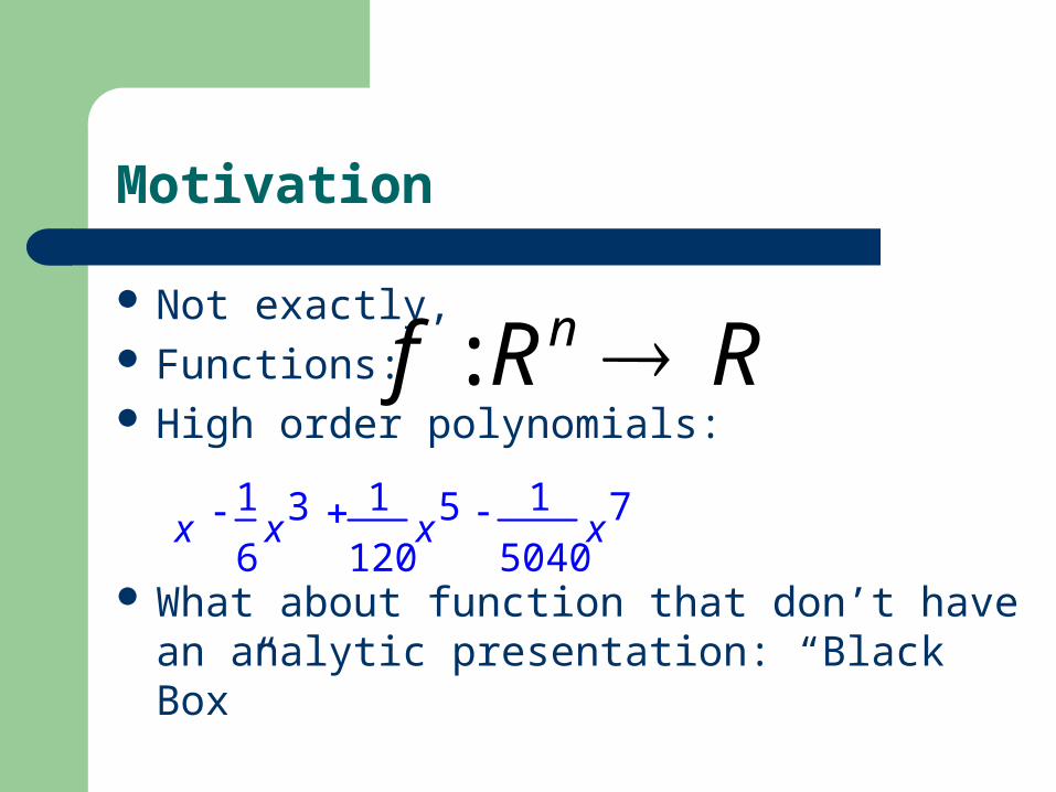
Not exactly, Functions: High order polynomials:

What about function that don’t have an analytic presentation: “Black Box”

x1

6x

3 1

120x

5 1

5040x

7

RRf n :

Motivation- “real world” problem

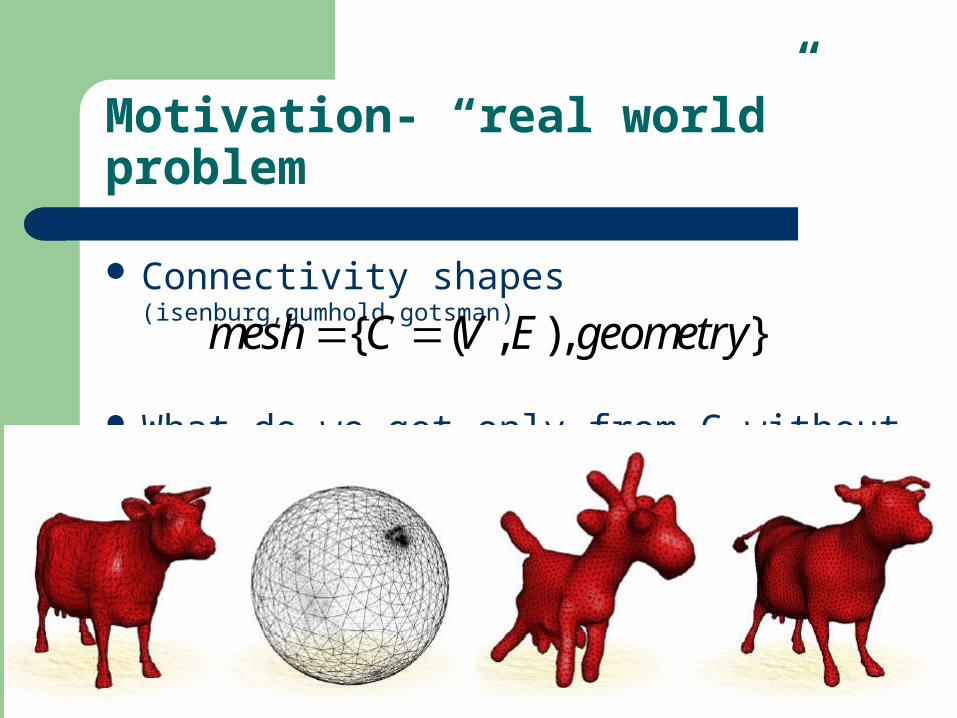
Connectivity shapes (isenburg,gumhold,gotsman)

What do we get only from C without geometry?

{ ( , ), }mesh C V E geometry

Motivation- “real world” problem

First we introduce error functionals and then try to minimize them:

23

( , )

( ) 1ns i j

i j E

E x x x

( , )

1( )i j i

i j Ei

L x x xd

3 2

1

( ) ( )n

nr i

i

E x L x

Motivation- “real world” problem

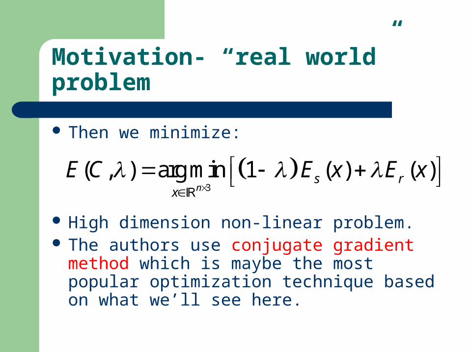
Then we minimize:

High dimension non-linear problem. The authors use conjugate gradient method

which is maybe the most popular optimization technique based on what we’ll see here.

3

( , ) arg min 1 ( ) ( )n

s rx

E C E x E x

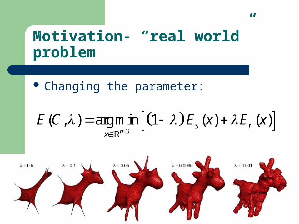
Motivation- “real world” problem

Changing the parameter:

3

( , ) arg min 1 ( ) ( )n

s rx

E C E x E x

Motivation

General problem: find global min(max) This lecture will concentrate on finding local

minimum.

Background

Motivation The gradient notion The Wolfe Theorems

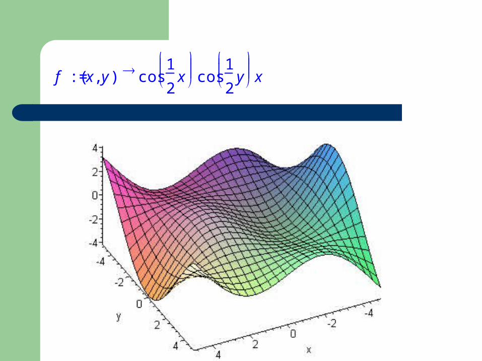
:= f ( ),x y

cos

1

2x

cos

1

2y x

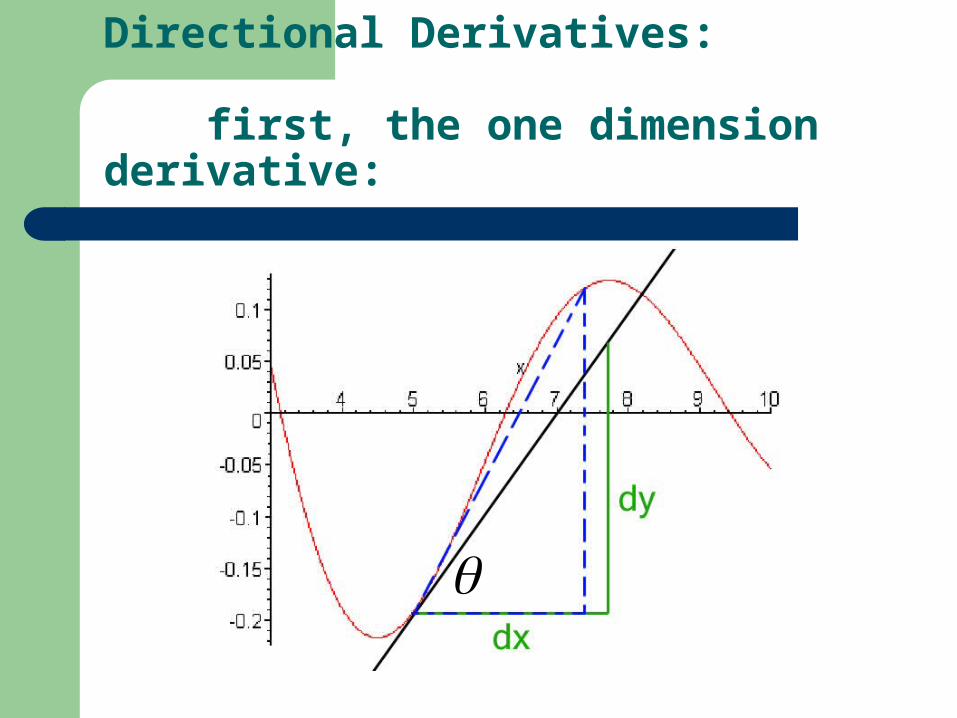
Directional Derivatives: first, the one dimension derivative:

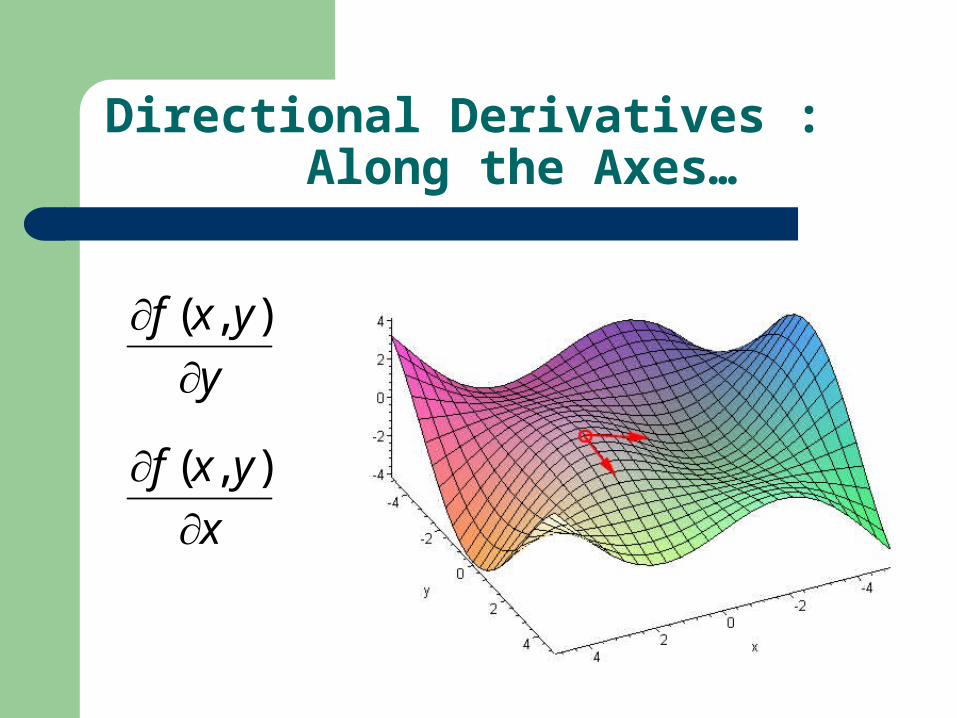
x

yxf

),(

y

yxf

),(

Directional Derivatives : Along the Axes…

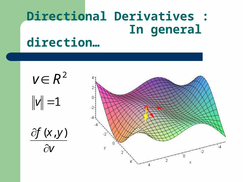
v

yxf

),(

2Rv

1v

Directional Derivatives : In general direction…

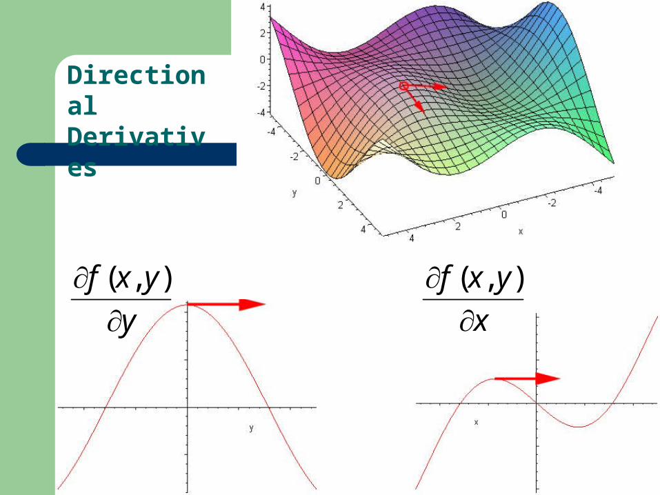
Directional Derivatives

x

yxf

),(

y

yxf

),(

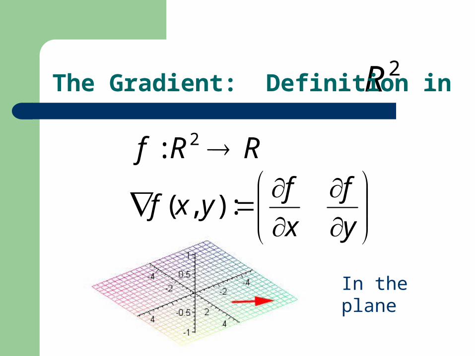
In the plane

2R

RRf 2:

y

f

x

fyxf :),(

The Gradient: Definition in

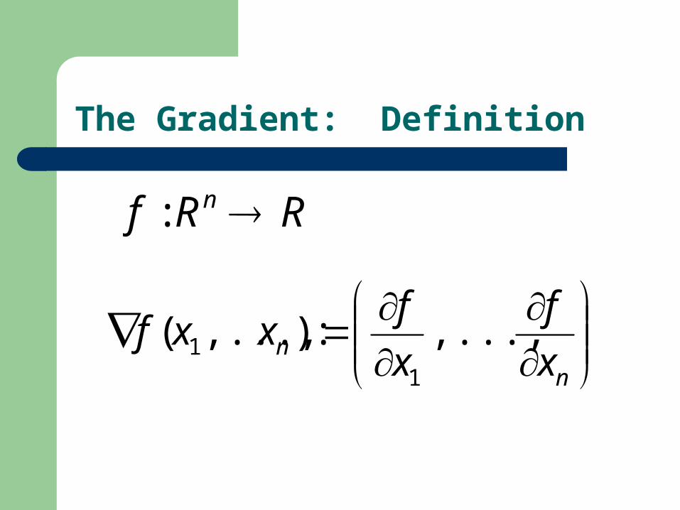
n

n x

f

x

fxxf ,...,:),...,(

11

RRf n :

The Gradient: Definition

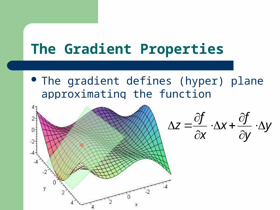
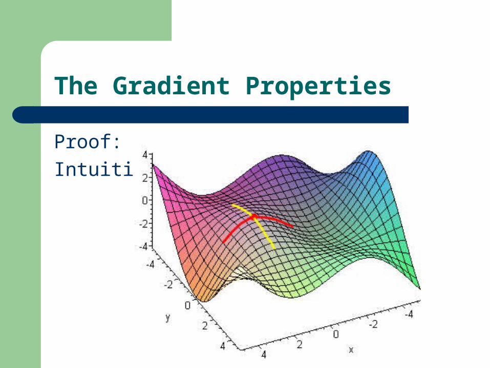
The Gradient Properties

The gradient defines (hyper) plane approximating the function infinitesimally

yy

fx

x

fz

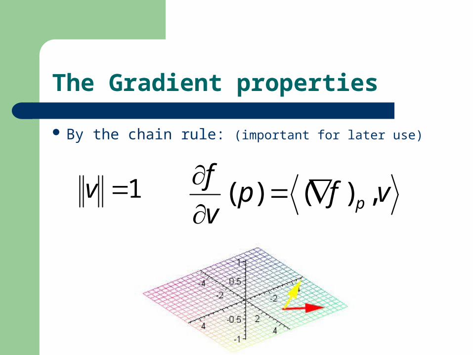
The Gradient properties

By the chain rule: (important for later use)

vfpv

fp ,)()(

1v

The Gradient properties

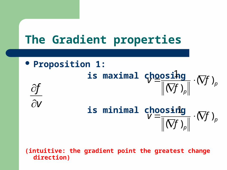
Proposition 1: is maximal choosing

is minimal choosing

(intuitive: the gradient point the greatest change direction)

v

f

p

p

ff

v )()(

1

p

p

ff

v )()(

1

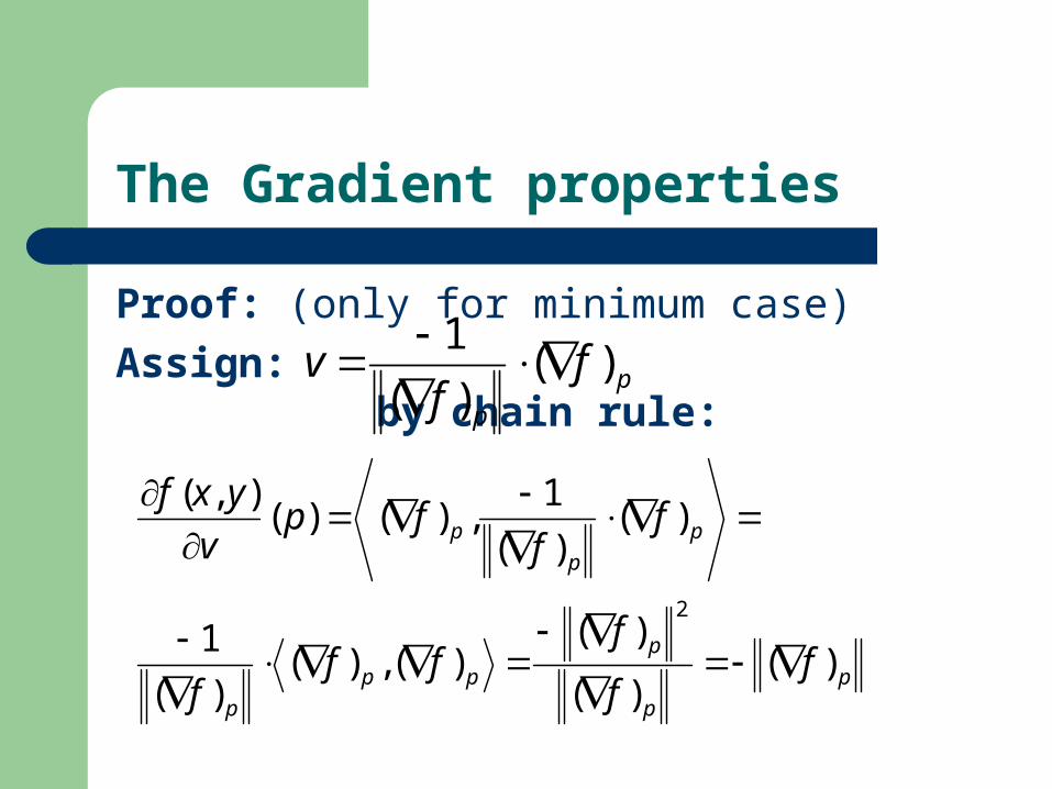
The Gradient properties

Proof: (only for minimum case)

Assign: by chain rule:

p

p

p

pp

p

p

p

p

ff

fff

f

ff

fpv

yxf

)()(

)()(,)(

)(

1

)()(

1,)()(

),(

2

p

p

ff

v )()(

1

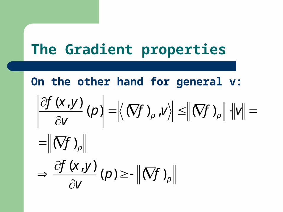
The Gradient properties

On the other hand for general v:

p

p

pp

fpv

yxf

f

vfvfpv

yxf

)()(),(

)(

)(,)()(),(

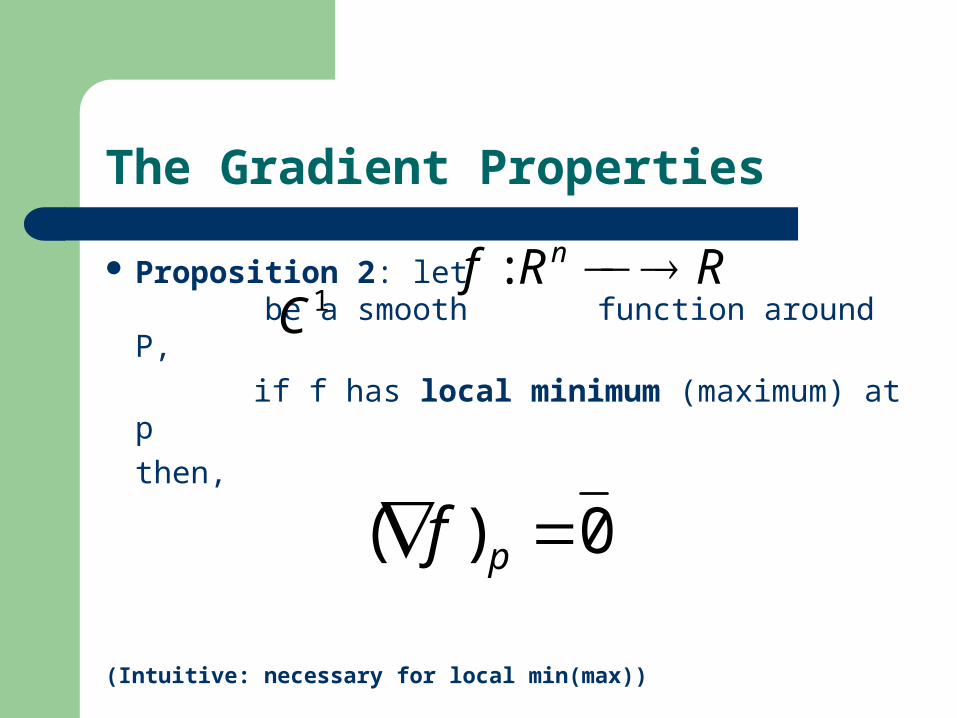
The Gradient Properties

Proposition 2: let be a smooth function around P,

if f has local minimum (maximum) at p

then,

(Intuitive: necessary for local min(max))

RRf n :

0)( pf

1C

The Gradient Properties

Proof:

Intuitive:

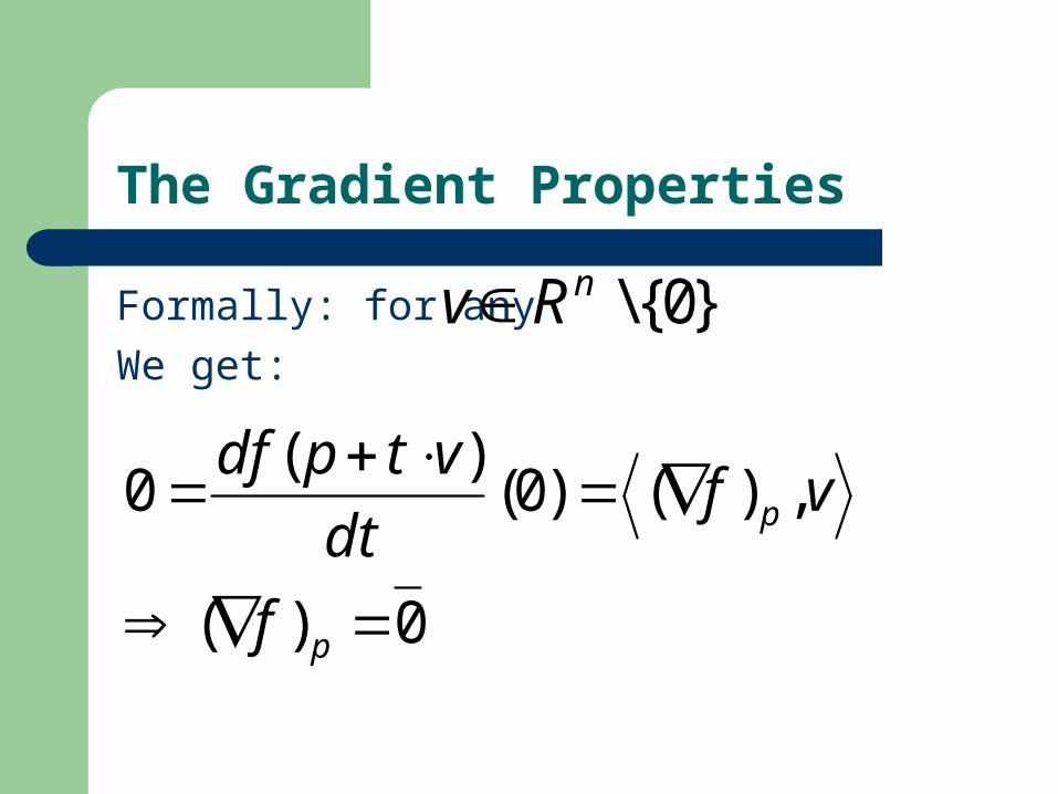
The Gradient Properties

Formally: for any

We get:}0{\nRv

0)(

,)()0()(

0

p

p

f

vfdt

vtpdf

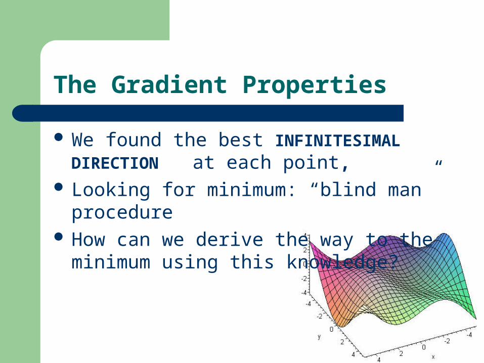
The Gradient Properties

We found the best INFINITESIMAL DIRECTION at each point,

Looking for minimum: “blind man” procedureHow can we derive the way to the minimum

using this knowledge?

Background

Motivation The gradient notion The Wolfe Theorems

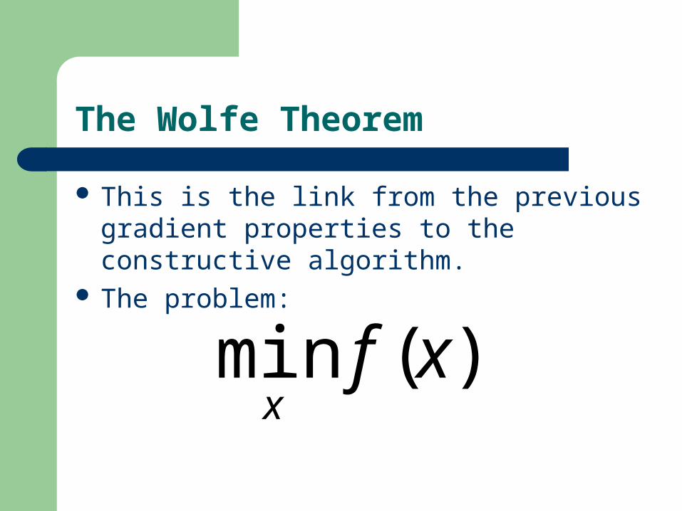
The Wolfe Theorem

This is the link from the previous gradient properties to the constructive algorithm.

The problem:

)(min xfx

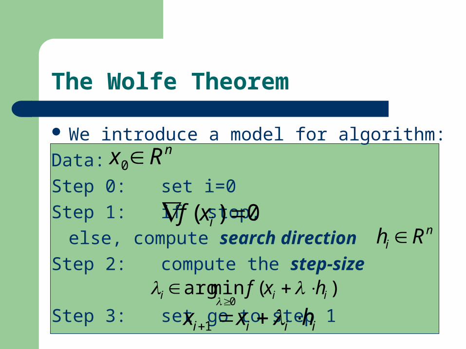
The Wolfe Theorem

We introduce a model for algorithm:

Data:

Step 0: set i=0

Step 1: if stop,

else, compute search direction

Step 2: compute the step-size

Step 3: set go to step 1

nRx 0

0)( ixfn

i Rh

)(minarg0

iii hxf

iiii hxx 1

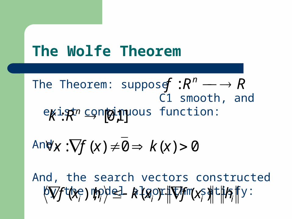
The Wolfe Theorem

The Theorem: suppose C1 smooth, and exist continuous function:

And,

And, the search vectors constructed by the model algorithm satisfy:

RRf n :

]1,0[: nRk

0)(0)(: xkxfx

iiiii hxfxkhxf )()(),(

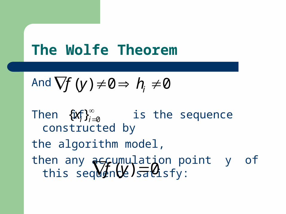
The Wolfe Theorem

And

Then if is the sequence constructed by

the algorithm model,

then any accumulation point y of this sequence satisfy:

0}{ iix

0)( yf

00)( ihyf

The Wolfe Theorem

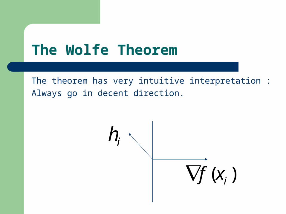
The theorem has very intuitive interpretation :

Always go in decent direction.

)( ixf

ih

Preview

Background Steepest DescentConjugate Gradient

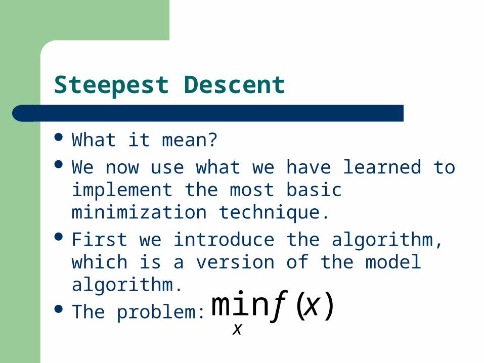
Steepest Descent

What it mean?We now use what we have learned to

implement the most basic minimization technique.

First we introduce the algorithm, which is a version of the model algorithm.

The problem: )(min xf

x

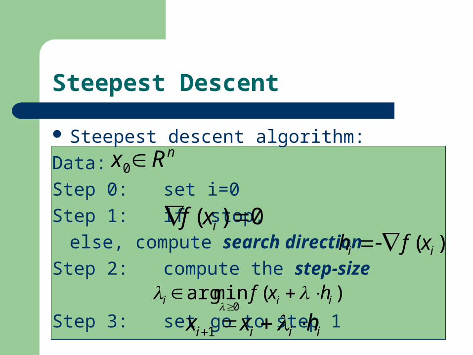
Steepest Descent

Steepest descent algorithm:

Data:

Step 0: set i=0

Step 1: if stop,

else, compute search direction

Step 2: compute the step-size

Step 3: set go to step 1

nRx 0

0)( ixf)( ii xfh

)(minarg0

iii hxf

iiii hxx 1

Steepest Descent

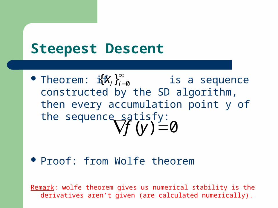
Theorem: if is a sequence constructed by the SD algorithm, then every accumulation point y of the sequence satisfy:

Proof: from Wolfe theorem

Remark: wolfe theorem gives us numerical stability is the derivatives aren’t given (are calculated numerically).

0)( yf

0}{ iix

Steepest Descent

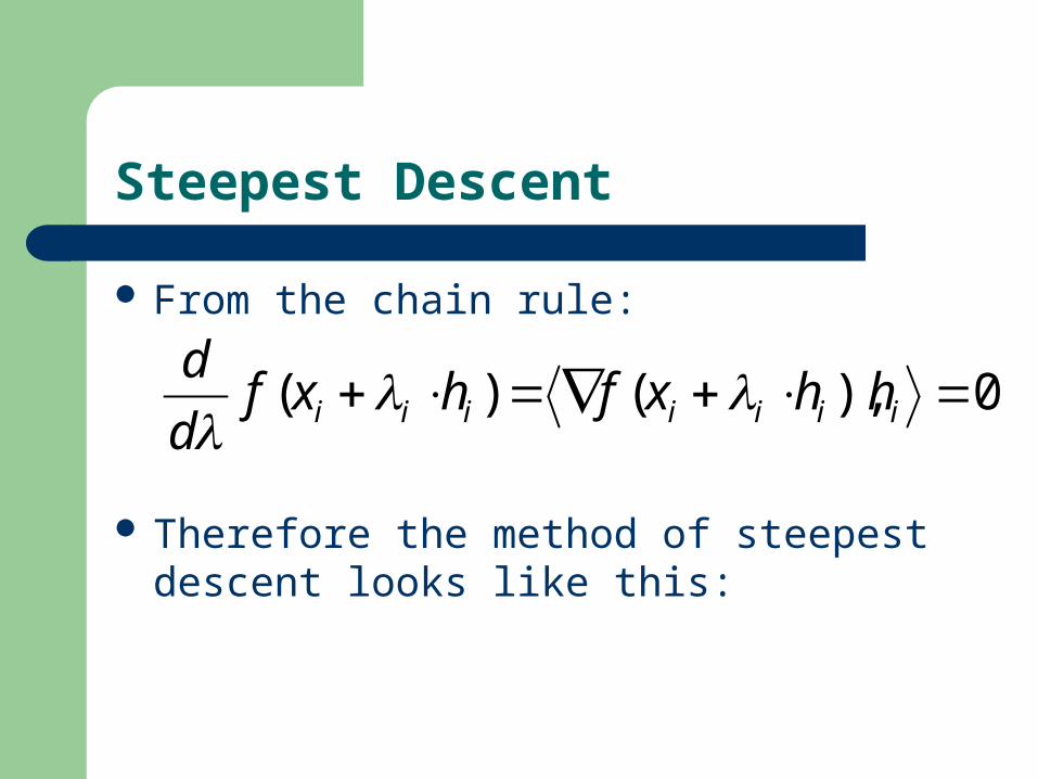
From the chain rule:

Therefore the method of steepest descent looks like this:

0),()( iiiiiii hhxfhxfd

d

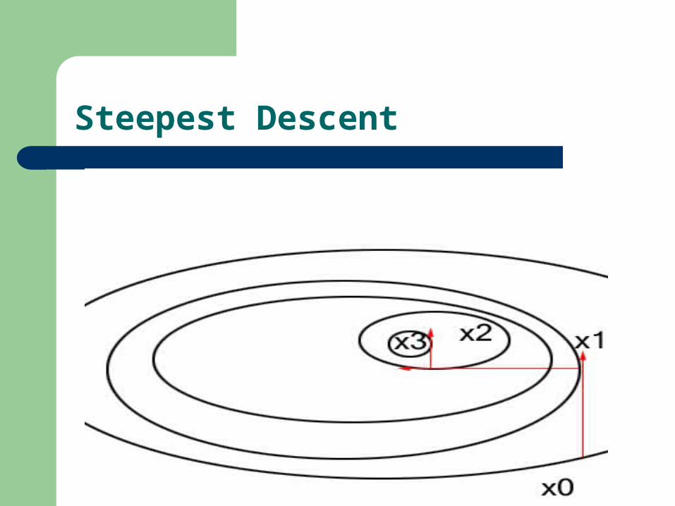
Steepest Descent

Steepest Descent

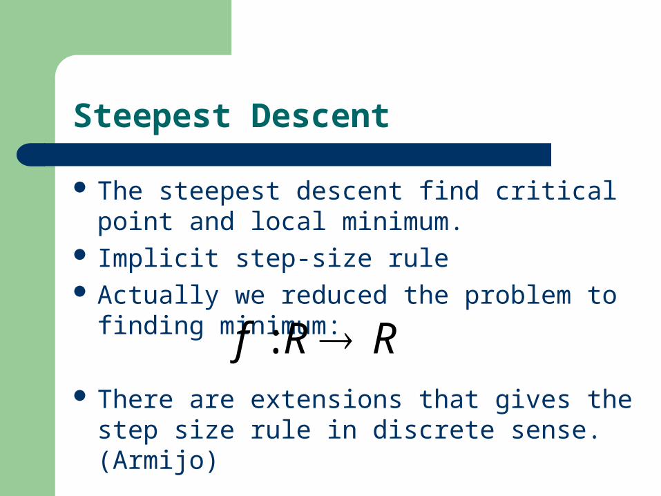
The steepest descent find critical point and local minimum.

Implicit step-size rule Actually we reduced the problem to finding

minimum:

There are extensions that gives the step size rule in discrete sense. (Armijo)

RRf :

Steepest Descent

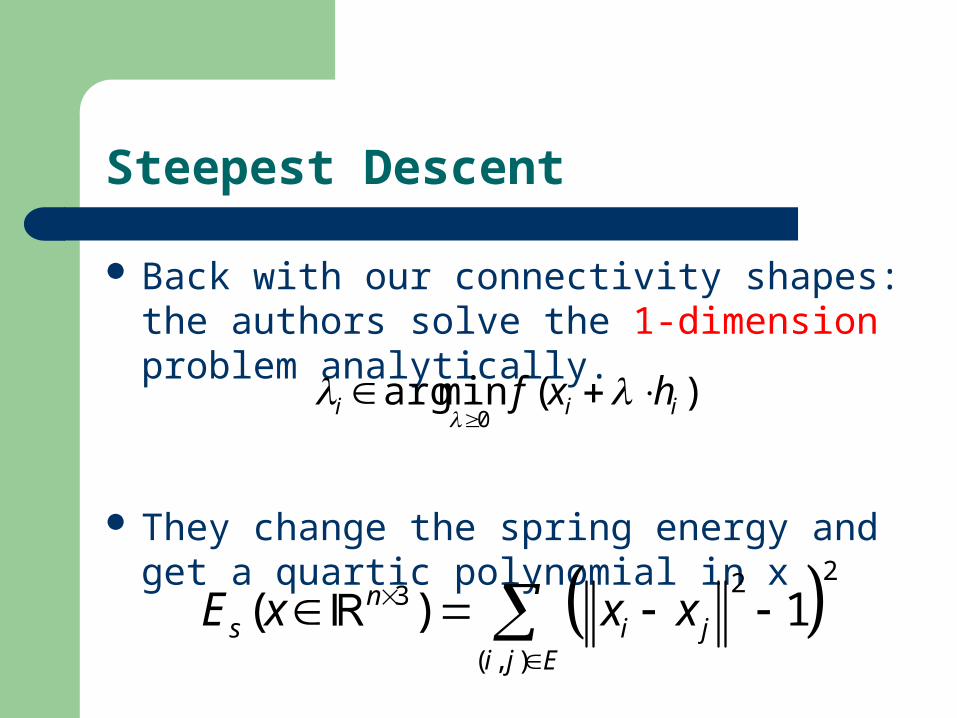
Back with our connectivity shapes: the authors solve the 1-dimension problem analytically.

They change the spring energy and get a quartic polynomial in x

)(minarg0

iii hxf

223

( , )

( ) 1ns i j

i j E

E x x x

Preview

Background Steepest DescentConjugate Gradient