graduate course - sol.du.ac.in · according to the present value method of capital budgeting, if...
TRANSCRIPT

Graduate Course Paper XIX Elective Group EA : Finance I
FINANCIAL AND INVESTMENT MANAGEMENT
FINANCIAL MANAGEMENT
Contents :
UNIT : 3
1. Cost of Capital – I
2. Cost of Capital – II
3. Capital Structure Theories
4. Capital Structure : Planning & Design
5. Financing Decision : EBIT-EPS Analysis
6. Financing Decision – Leverage Analysis
UNIT : 4
1. Dividend Decision and Valuation of the Firm
2. Dividend Policy : Determinants and Constraints
UNIT : 5
1. Working Capital : Management and Finance
2. Working Capital : Estimation and Calculation
3. Financing of Working Capital
4. Management of Cash
5. Receivable Management
6. Inventory Management
Editor :
K.B. Gupta
SCHOOL OF OPEN LEARNING UNIVERSITY OF DELHI
5, CAVALRY LANE
DELHI-110007
SESSION 2007-08
©School of Open Leaning
Published by the Executive Director, School of Open Learning, University of
Delhi, 5 Cavalry Lane, Delhi-110007.
Laser typeset : S.O.L. Computer Centre
Printed at :

UNIT 3
1
COST OF CAPITAL- I
Smriti Chawla
Shri Ram College of Commerce University of Delhi
Meaning, Concept and Definition
The cost of capital of a firm is the minimum rate of return expected by its investors. It is
the weighted average cost of various sources of finance used by a firm. The capital used by a
firm may be in the form of debt, preference capital, retained earnings and equity shares. The
concept of cost of capital is very important in the financial management. A decision to invest in a
particular project depends upon the cost of capital of the firm or the cut off rate which is the
minimum rate of return expected by the investors. In case a firm is not able to achieve even the
cut off rate, the market value of its shares will fall. In fact cost of capital is the minimum rate of
return expected by its investors which will maintain the market value of shares at its present
level. Hence to achieve the objective of wealth maximisation, a firm must earn a rate of return
more than its cost of capital. The cost of capital of a firm or the minimum rate of return expected
by its investors has a direct relation with the risk involved in the firm. Generally, higher the risk
involved in a firm, higher is the cost of capital.
According to Solomon Ezra Cost of capital is the minimum required rate of earnings or
the cut-off rate of capital expenditures.
Thus, we can say that cost of capital is that minimum rate of return which a firm, and, is
expected to earn on its investments so as to maintain the market value of its shares.
From the definitions given above we can conclude three basic aspects of the concept of cost of
capital:
CHAPTER OBJECTIVES
� Understand the Meaning, Concept and Significance of Cost of Capital.
� Classification of Cost
� Problems in Determining the Cost of Capital � Computation of Specific Source of Finance
Cost of Debt Cost of Preference Capital Cost of Equity Share Capital
Cost of Retained Earnings � Illustrations

2
(i) Cost of capital is not a cost as such. In fact, it is the rate of return that a firm requires
to earn from its projects.
(ii) It is the minimum rate of return. Cost of capital of a firm is that minimum rate of
return which will at least maintain the market value of the shares.
(iii) It comprises of three components. As there is always some business and financial risk
in investing funds in a firm, cost of capital comprises of three components:
(a) the expected normal rate of return at zero risk level, say the rate of interest
allowed by banks;
(b) the premium for business risk; and
(c) the premium for financial risk on account of pattern of capital structure.
Symbolically cost of capital may be represented as:
where, K = ro+b+f
K=Cost of capital
ro=Normal rate of return at zero risk level
b=Premium for business risk.
f=Premium for financial risk.
Significance of the Cost of Capital
The concept of cost of capital is very important in the financial management. It plays a
crucial role in both capital budgeting as well as decisions relating to planning of capital structure.
Cost of capital concept can also be used as a basis for evaluating the performance of a firm and it
further helps management in taking so many other financial decisions.
(1) As an Acceptance Criterion in Capital Budgeting: Capital budgeting decisions can be made
by considering the cost of capital. According to the present value method of capital budgeting, if
the present value of expected returns from investment is greater than or equal to the cost of
investment, the project may be accepted; otherwise the project may be rejected. The present
value of expected return is calculated by discounting the expected cash inflows at cut-off rate
(which is the cost of capital). Hence, the concept of cost of capital is very useful in capital
budgeting decision.
(2) As a Determinant of Capital Mix in Capital Structure Decisions: Financing the firm’s
assets is a very crucial problem in every business and as a general rule there should be a proper
mix of debt and equity capital in financing a firm’s assets. While designing an optimal capital
structure, the management has to keep in mind the objective or maximising the value of the firm
and minimising the cost of capital. Measurement of cost of capital from various sources is very
essential in planning the capital structure of any firm.
(3) As a basis for evaluating the Financial Performance: The concept of cost of capital can be
used to ‘evaluate the financial performance of top management’. The actual profitability of the
project is compared to the projected overall cost of capital and the actual cost of capital of funds
raised to finance the project. If the actual profitability of the project is more than the projected
and the actual cost of capital, the performance may be said to be satisfactory.
(4) As a Basis for taking other Financial Decisions: The cost of capital is also used in making
other financial decisions such as dividend policy, capitalisation of profits, making the rights issue
and working capital.

3
Classification of Cost
(1) Historical cost and Future Cost: Historical costs are book costs which are related to the past.
Future costs are estimated costs for the future. In financial decisions future costs are more
relevant than the historical costs. However, historical costs act as guide for the estimation of
future costs.
(2) Specific Cost and Composite Cost: Specific cost refers to the cost of a specific source of
capital while composite cost is combined cost of various sources of capital. It is the weighted
average cost of capital. In case more than one form of capital is used in the business, it is the
composite cost which should be considered for decision-making and not the specific cost. But
where only one type of capital is employed the specific cost of that type of capital may be
considered.
(3) Explicit Cost and Implicit Cost: An explicit cost is the discount rate which equates the
present value of cash inflows with the present of cash outflows. In other words it is the internal
rate of return.
( ) ( ) ( ) ( )
∑− +
=+
++
++
=n
t
t
t
n
n
o
K
O
k
O
k
O
K
OI
12
21
11..................................
11
where, Io, is the net cash inflow at zero point of time,
Ot is the outflow of cash in period 1, 2 and n.
k is the explicit cost of capital.
Implicit cost also known as the opportunity cost is the cost of the opportunity foregone is order
to take up a particular project.
(4) Average Cost and Marginal Cost: An average cost refers to the combined cost of various
sources of capital such as debentures, preference shares and equity shares. It is the weighted
average cost of the costs of various sources of finance. Marginal cost of capital refers to the
average cost of capital which has to be incurred to obtain additional funds required by a firm. In
investment decisions, it is the marginal cost which should be taken into consideration.
Determination of Cost of Capital
It has already been stated that the cost of capital plays a crucial role in the decisions
relating to financial management. However, the determination of the cost of capital of a firm is
not an easy task because of both conceptual problems as well as uncertainties of proposed
investments and the pattern of financing. The major problems concerning the determination of
cost of capital are discussed as below:
Problems in determining Cost of Capital
1. Conceptual controversies regarding the relationship between the cost of capital and
the capital structure : Different theories have been propounded by different authors explaining
the relationship between capital structure, cost of capital and the value of the firm. This has
resulted into various conceptual difficulties. According to the Net Income Approach and the
traditional theories both the cost of capital as well the value of the firm have a direct relationship
with the method and level of financing. In their opinion, a firm can minimise the weighted
average cost of capital and increase the value of the firm by using debt financing. On the other
4
hand, Net Operating Income and Modigliani and Miller Approach prove that the cost of capital is
not affected by changes in the capital structure or say that debt equity mix is irrelevant in
determination of cost of capital structure determination of cost of capital and the value of a firm.
However, the M and M approach is based upon certain unrealistic assumptions such as, there is a
perfect market or the expected earnings of all the firms have identical risk characteristic, etc.
2. Problems in computation of cost of equity: The computation of cost of equity capital
depends upon the expected rate of return by its investors. But the quantification of the
expectations of equity shareholders is a very difficult task because there are many factors which
influence their valuation about a firm.
3. Problems in computation of cost of retained earnings: It is sometimes argued that
retained earnings do not involve any cost but in reality, it is the opportunity cost of dividends
foregone by its shareholders. Since different shareholders may have different opportunities for
investing their dividends, it becomes very difficult to compute the cost of retained earnings.
4. Problems in assigning weights: For determining the weighted average cost of capital,
weights have to be assigned to the specific cost of individual source of finance. The choice of
using the book value of the source or the market value of the source poses another problem in the
determination of capital.
COMPUTATION OF SPECIFIC SOURCE OF FINANCE
Computation of each specific source of finance, viz, debt, preference share capital equity
share capital and retained earnings is discussed as below:
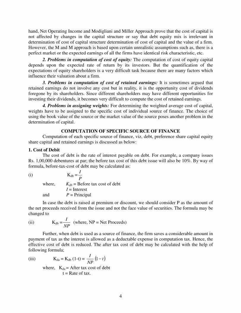
1. Cost of Debit
The cost of debt is the rate of interest payable on debt. For example, a company issues
Rs. 1,00,000 debentures at par; the before tax cost of this debt issue will also be 10%. By way of
formula, before-tax-cost of debt may be calculated as:
(i) Kdb =P
I
where, Kdb = Before tax cost of debt
I = Interest
and P = Principal
In case the debt is raised at premium or discount, we should consider P as the amount of
the net proceeds received from the issue and not the face value of securities. The formula may be
changed to
(ii) Kdb =NP
I (where, NP = Net Proceeds)
Further, when debt is used as a source of finance, the firm saves a considerable amount in
payment of tax as the interest is allowed as a deductable expense in computation tax. Hence, the
effective cost of debt is reduced. The after tax cost of debt may be calculated with the help of
following formula;
(iii) Kda = Kdb (1-t) = ( )tNP
I−1
where, Kda = After tax cost of debt
t = Rate of tax.

5
Cost of Redeemable Debt Usually, the debt is issued to be redeemed after a certain period during lifetime of a firm.
Such a debt issue is known as Redeemable debt. The cost of redeemable debt capital be
computed as:
(iv) Before-tax cost of debt
( )
( )NPP
NPPn
I
Kdb
+
−+
=
2
1
1
where, I = Interest
N = Number of years in which debt is to be redeemed
P = Proceeds at par
NP = Net Proceeds
(v) After tax cost of debt, Kda = Kdb (1-t)
where,
( )
( )NPP
NPPn
I
Kdb
+
−+
=
2
1
1
Illustration1: A Company issues shares of Rs.10,00,000, 10% redeemable debentures at
a discount of 5%. The cost of floatation amount to Rs.30,000. The debentures are redeemable
after 5 years. Calculate before tax and after tax cost of debt assuming tax rate of 50%.
Solution:
Before-tax cost of debt,
( )
( )NPP
NPPn
I
Kdb
+
−+
=
2
1
1
=
( )
( )000,0,9000,00,102
1
000,20,9000,00,105
1000,00,1
+
−+
(NP=Rs. 10,00,000-50,000 (discount) – 30,000 cost of floatation)
= %09.12000,60,9
000,16,1
000,60,9
000,16000,00,1==
+
After tax cost of debt, Kda = Kdb (1-0.5)
= 12.09 (1-0.5) = 6.04%
Cost of Debt Redeemable at Premium
Sometimes debentures are to be redeemed at a premium; i.e at more than the face value
after the expiry of a certain period. The cost of such debt redeemable at premium can be
computed as below:

6
(i) Before tax cost of debt,
( )
( )NPRV
NPRVn
I
Kdb
+
−+
=
2
1
1
where, I = Interest
n = Number of years in which debt is to be redeemed
RV= Redeemable value of debt
NP = Net Proceeds
(ii) After-tax cost of debt,
Kda= Kdb (1-t)
Illustration2: A 5-year Rs.100 debenture of a firm can be sold for a net price of
Rs.96.50. The coupon rate of interest is 14 %per annum and debenture will be redeemed at 5%
premium on maturity. The firm tax rate is 40%. Compute the after tax cost of debentures.
Solution:
( )
( )NPRV
NPRVn
I
Kdb
+
−+
=
2
1
1
=
( )
( )%58.15
75.100
70.15
50.961052
1
50.961055
114
==
+
−+
After-tax cost of debt,
Kda = Kdb (1-t)
= 15.58 (1-0.4) = 15.58 x 0.6 = 9.35%
Cost of Debt Redeemable in Instalments
Financial institutions generally require principal to be amortised in instalments. A
company may also issue a bond or debenture to be redeemed periodically. In such a case,
principal amount is repaid each period instead of a lump sum at maturity and hence cash period
include interest and principal. The amount of interest goes on decreasing each period as it is
calculated on decreasing each period as it is calculated on the outstanding amount of debt. The
before-tax cost of such a debt can be calculated as below:
( ) ( ) ( )n
d
nn
dd
d
KI
PI
KI
PI
K
PIV
+
+++
+
++
+
+= ................
12
22
1
11
or, Vd = ( )
∑− +
+n
t
t
d
tt
KI
PI
1
where, Vd = Present value of bond or debt
I1, I2....In = Annual interest (Rs.) in period 1,2... and so on.
P1,P2...Pn=Periodic payment of principal in period 1, 2, and so on.

7
n = Number of years to maturity
Kd = Cost of debt or Required rate of return.
Cost of Existing Debt
If a firm wants to compute the current cost of its existing debt, the current market yield of
the debt should be taken into consideration. Suppose a firm has 10% debentures of Rs. 100 each
outstanding on January 1, 1994 to be redeemed on December 31, 2000 and the new debentures
could be issued at a net realisable price of Rs. 90 in the beginning of 1996, the current cost of
existing debt will be computed as:
( )
( )901002
1
901005
110
+
−+
=db
K = %63.1295
12=
Further, if the firm’s tax rate is 40% the after-tax cost of debt will be:
Kda = Kdb (1-t)
= 12.63 (1-0.4)
= 7.58%
Cost of Zero Coupon Bonds
Sometimes companies issue bonds or debentures at a discount from their eventual maturity
value and having zero interest rate. No interest is payable on such debentures before their
redemption and at the time of redemption the maturity value of the bond is to be paid to the
investors. The cost of such debt can be calculated by finding the present values of cash flows as
below:
(i) Prepare the cash flow table using an arbitrary assumed discount rate to discount the
cash flows to the present value.
(ii) Find out the net present value by deducting the present value of the outflows from the
present value of the inflows.
(iii) If the net present value is positive apply higher rate of discount.
(iv) If the higher discount rate still gives a positive net present value increase the discount
rate further until the UPV becomes negative.
(v) If the NPV is negative at this higher rate the cost of debt must be between these two
rates.
Illustration 3: X Ltd. has issued redeemable zero coupon bonds of Rs. 100 each at a discount
rate of Rs. 60 repayable at the end of fourth year. Calculate the cost of debt.
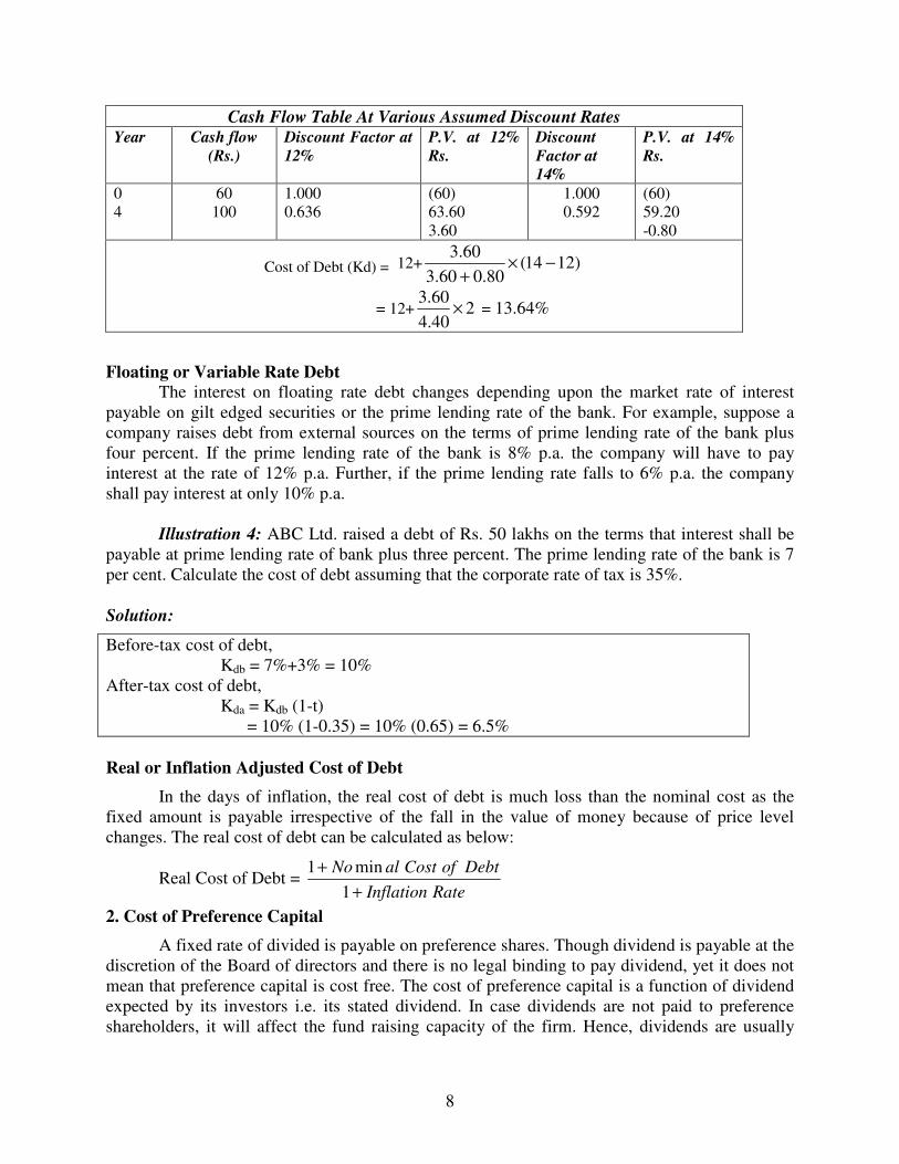
8
Cash Flow Table At Various Assumed Discount Rates
Year Cash flow
(Rs.)
Discount Factor at
12%
P.V. at 12%
Rs.
Discount
Factor at
14%
P.V. at 14%
Rs.
0
4
60
100
1.000
0.636
(60)
63.60
3.60
1.000
0.592
(60)
59.20
-0.80
Cost of Debt (Kd) = 12+ )1214(80.060.3
60.3−×
+
= 12+ 240.4
60.3× = 13.64%
Floating or Variable Rate Debt
The interest on floating rate debt changes depending upon the market rate of interest
payable on gilt edged securities or the prime lending rate of the bank. For example, suppose a
company raises debt from external sources on the terms of prime lending rate of the bank plus
four percent. If the prime lending rate of the bank is 8% p.a. the company will have to pay
interest at the rate of 12% p.a. Further, if the prime lending rate falls to 6% p.a. the company
shall pay interest at only 10% p.a.
Illustration 4: ABC Ltd. raised a debt of Rs. 50 lakhs on the terms that interest shall be
payable at prime lending rate of bank plus three percent. The prime lending rate of the bank is 7
per cent. Calculate the cost of debt assuming that the corporate rate of tax is 35%.
Solution:
Before-tax cost of debt,
Kdb = 7%+3% = 10%
After-tax cost of debt,
Kda = Kdb (1-t)
= 10% (1-0.35) = 10% (0.65) = 6.5%
Real or Inflation Adjusted Cost of Debt
In the days of inflation, the real cost of debt is much loss than the nominal cost as the
fixed amount is payable irrespective of the fall in the value of money because of price level
changes. The real cost of debt can be calculated as below:
Real Cost of Debt = RateInflation
DebtofCostalNo
+
+
1
min1
2. Cost of Preference Capital
A fixed rate of divided is payable on preference shares. Though dividend is payable at the
discretion of the Board of directors and there is no legal binding to pay dividend, yet it does not
mean that preference capital is cost free. The cost of preference capital is a function of dividend
expected by its investors i.e. its stated dividend. In case dividends are not paid to preference
shareholders, it will affect the fund raising capacity of the firm. Hence, dividends are usually

9
paid regularly on preference shares except when there are no profits to pay dividends. The cost
of preference capital which is perpetual can be calculated as:
Kp = P
D
where Kp = Cost of Preference Capital
D = Annual Preference Dividend
P = Preference Share Capital (Proceeds.)
Further, if preference shares are issued at Premium or Discount or when costs of
floatation are incurred to issue preference shares, the nominal or par value of preference share
capital has to be adjusted to find out the net proceeds from the issue of preference shares. In such
a case, the cost of preference capital can be computed with the following formula:
Kp = NP
D
It may be noted that as dividend are not allowed to be deducted in computation of tax, no
adjustment is required for taxes.
Sometimes Redeemable Preference Shares are issued which can be redeemed or
cancelled on maturity date. The cost of redeemable preference share capital can be calculated as:
( )NPMV
n
NPMVD
Kpr
+
−+
=
2
1
where, Kpr = Cost of Redeemable Preference Shares
D = Annual Preference dividend
MV = Maturity Value of Preference Shares
NP = Net proceeds of Preference Shares
Illustration 5: A company issues 10,000 shares 10% Preference Shares of Rs. 100 each. Cost of
issue is Rs. 2 per share. Calculate cost of preference capital if these shares are issued (a) at par,
(b) at a premium of 10% and (c) at a discount of 5%.
Solution:
Cost of Preference Capital, Kp = NP
D
(a) %2.10100000,80,9
000,00,1100
000,20000,00,10
000,00,1=×=×
−=
pK
(b) 100000,20000,00,1000,00,10
000,00,1×
−+=
PK = 100
000,80,10
000,00,1×
= 9.26%
(c) 100000,20000,50000,00,10
000,00,1×
−−=
PK = 100
000,30,9
000,00,1×
=10.75%

10
3. Cost of Equity Share Capital
The cost of equity is the maximum rate of return that the company must earn on equity
financed portion of its investments in order to leave unchanged the market price of its stock.’
The cost of equity capital is function of the expected return by its investors. The cost of equity is
not the out-of-pocket cost of using equity capital as the equity shareholders are not paid dividend
at a fixed rate every year. Moreover, payment of dividend is not a legal binding. It may or may
not be paid. But it does not mean that equity share capital is a cost free capital. The cost of equity
can be computed in following ways:
(a) Dividend Yield Method or Dividend/Price Ratio Method : According to this method,
the cost of equity capital is the ‘discount rate that equates the present value of expected future
dividends per share with the net proceeds (or current market price) or a share’. Symbolically.
Ke = MP
Dor
NP
D
where, Ke = Cost of Equity Capital
D = Expected dividend per share
NP = net proceeds per share
and MP = Market Price per share.
Illustration 6: A company issues 1000 equity shares of Rs. 100 each at a premium of 10%. The
company has been paying 20% dividend to equity shareholders for the past five years and
expects to maintain the same in the future also. Compute the cost of equity capital, Will it make
any difference if the market price of equity share is Rs. 160?
Solution:
Ke = NP
D
= %18.18100x110
20=
If the market price of a equity share is Rs. 160
Ke = MP
D
= %5.12100x160
20=
(b) Dividend yield plus growth in dividend method : When the dividends of the firm are
expected to grow at a constant rate and the dividend pay out ratio is constant this method may be
used to compute the cost of equity capital. According to this method the cost of equity capital is
based on the dividends and the growth rate.
Ke = ( )
GNP
gDG
NP
DO +
+=+
11
where, Ke = Cost of equity capital
D1 = Expected Dividend per share at the end of the year
NP = Net proceeds per share
G = Rate of growth in dividends
Do = previous year’s dividend.

11
Further, in case cost of existing equity share capital is to be calculated, the NP should be
changed with MP (market price per share) in the above equation.
Ke = GMP
D+1
Illustration7: (a) A company plans to issue 1000 new shares of Rs. 100 each at par. The
floatation costs are expected to be 5% of the share price. The company pays a dividend of Rs. 10
per share initially and the growth in dividends is expected to be 5%. Compute the cost of new
issue of equity shares.
(b) If the current market price of an equity share is Rs. 150, calculate the cost of existing equity
share capital.
Solution:
(a) Ke = GNP
D+
= %53.15%55100
10=+
−
(b) Ke = GMP
D+
= %67.11%5150
10=+
(c) Earning Yield Method : According to this method, the cost of equity capital is the
discount rate that equates the present values of expected future earnings per share with the net
proceeds (or, current market price) of a share. Symbolically:
Ke = oceedsNet
shareperEarnings
Pr
= NP
EPS
where, the cost of existing capital is to be calculated:
Ke = SharePericeMarket
shareperEarnings
Pr
= MP
EPS
(d) Realised Yield Method: One of the serious limitations of using dividend yield method
or earnings yield method is the problem of estimating the expectations of the investors regarding
future dividends and earnings. It is not possible to estimate future dividends and earnings
correctly; both of these depend upon so many uncertain factors. To remove this drawback,
realised yield method which takes into account the actual average rate of return realised in the
past may be applied to compute the cost of equity share capital. To calculate the average rate of
return realised, dividend received in the past along with the gain realised at the time of sale of
shares should be considered. The cost of equity capital is said to be the realised rate of return by
the shareholders. This method of computing cost of equity share capital is based upon the
following assumptions:

12
(a) The firm will remain in the same risk class over the period.
(b) The shareholders expectations are based upon the past realised yield.
(c) The investors get the same rate of return as the realised yield even if they invest elsewhere;
(d) The market price of shares does not change significantly.
4. Cost of Retained Earning
It is sometimes argued that retained earnings do not involve any cost because a firm is not
required to pay dividends on retained earnings. However, the shareholders expect a return on
retained profits. Retained earnings accrue to a firm only because of some sacrifice made by the
shareholders in not receiving the dividends out of the available profits.
The cost of retained earnings may be considered as the rate of return which the existing
shareholders can obtain by investing the after tax dividends in alternative opportunity of equal
qualities. It is, thus, the opportunity cost of dividends foregone by the shareholders. Cost of
retained earnings can be computed with the help of following formula:
Kr = GNP
D+
where,
Kr = Cost of retained earnings
D = Expected dividend
NP = Not proceeds of share issue
G = Rate of growth.

13
2
COST OF CAPITAL – II
Smriti Chawla Shri Ram College of Commerce
University of Delhi
Computation of Weighted Average Cost of Capital
Weighted average cost of capital is the average cost of the costs of various source of
financing. Weighted average cost of capital is also known as composite cost of capital, overall
cost of capital or average cost of capital. Once the specific cost of individual sources of finance
is determined, we can compute the weighted average cost of capital by putting weights to the
specific costs of capital in proportion of various sources of funds to total. The weights may be
given either by using the book value of source or market value of source. If there is a difference
between market value and book value weights, the weights, the weighted average cost of capital
would also differ. The market value weighted average cost would be overstated if market value
of the share is higher than book value and vice versa. The market value weights are sometimes
preferred to the book value weights because the market value represents the true value of
investors. However, the market value weights suffer from the following limitations:
(i) It is very difficult to determine the market values because of frequent fluctuations.
(ii) With the use of market value weights, equity capital gets greater importance.
For the above limitations, it is better to use book value which is readily available. Weighted
average cost of capital can be computed as follows:
Kw = W
XW
∑
∑
Kw = Weighted average cost of capital
X = Cost of specific source of finance
CHAPTER OBJECTIVES
� Computation of weighted average cost of capital
� Marginal cost of capital � Cost of Equity using Capital Asset Pricing Model
� Illustrations � Lets Sum Up
� Questions

14
W = Weight, proportion of specific source of finance
Illustration1: A firm has the following capital structure and after-tax costs for the different
sources of funds used:
Source of Funds Amount
Rs.
Proportion
%
After-tax cost
%
Debt
Preference Shares
Equity Shares
Retained Earnings
Total
15,00,000
12,00,000
18,00,000
15,00,000
60,00,000
25
20
30
25
100
5
10
12
11
You are required to compute the weighted average cost of capital.
Solution:
Computation of Weighted Average Cost of Capital
Source of Funds Proportion %
(W)
Cost %
(X)
Weighted Cost %
Proportion ×Cost
(XW) %
Debt
Preference shares
Equity Shares
Retained Earnings
25
20
30
25
5
10
12
11
1.25
2.00
3.60
2.75
Weighted Average Cost of
Capital
9.60%
Illustration2: Continuing illustration 1, the firm has 18,000 equity shares of Rs. 100 each
outstanding and the current market price is Rs. 300 per calculate the market, value weighted
average cost of capital assuming that the market values and book values of the debt and
preference capital are same.
Solution:
Sources of Funds
Amount
(Rs.)
Proportion %
W
Cost
% X
Weighted Cost
Proportion ×
Cost XW
Debt
Preference Capital
Equity Share Capital
(18000 shares @ Rs. 300)
15,00,000
12,00,000
54,00,000
81,00,000
18.52
14.81
66.67
100
5
10
12
0.93
1.48
8.00
Weighted Average Cost of Capital 10.41%
Marginal Cost of Capital
The marginal cost of capital is the weighted average cost of new capital calculated by
using the marginal weights. The marginal weights represent the proportion of various sources of
funds to be employed in raising additional funds. In case, a firm employs the existing proportion

15
of capital structure and the component costs remain the same the marginal cost of capital shall be
equal to the weighted average cost of capital. But in practice, the proportion and /or the
component costs may change for additional funds to be raised. Under this situation the marginal
cost of capital shall not be equal to weighted average cost of capital. However, the marginal cost
of capital concept ignores the long-term implications of the new financing plans, and thus,
weighted average cost of capital should be preferred for maximisation of shareholder’s wealth in
the long-run.
Illustration3: A firm has the following capital structure and after-tax costs for the different
sources of funds used:
Source of Funds Amount (Rs.) Proportion (%) After-tax Cost (%)
Debt
Preference Capital
Equity Capital
4,50,000
3,75,000
6,75,000
15,00,000
30
25
45
100
7
10
15
(a) Calculate the weighted average cost of capital using book-value weights.
(b) The firm wishes to raise further Rs. 6,00,000 for the expansion of the project as below.
Debt Rs. 3,00,000
Preference Capital Rs. 1,50,000
Equity Capital Rs. 1,50,000
Assuming that specific costs do not change, compute the weighted marginal cost of capital.
Solution:
Computation of Weighted Average Cost of Capital (WACC)
Source of Funds Proportion (%) (W) After tax cost (%)
(X)
Weighted Cost %
(XW) %
Debt
Preference Capital
Equity Capital
30
25
45
7
10
15
2.10
2.50
6.75
Weighted Average Cost of Capital (WACC) 11.35%
Computation of Weighted Marginal Cost of Capital (WMCC)
Source of Funds Marginal Weights
Proportion (%) (W)
After tax cost (%)
(X)
Weighted Marginal
Cost %
Debt
Preference Capital
Equity Capital
50
25
25
7
10
15
3.50
2.50
3.75
Weighted Marginal Cost of Capital (WMCC) 9.75%
Cost of Equity Using Capital Asset Pricing Model (CAPM)
The value of an equity share is a function of cash inflows expected by the investors and risk
associated with cash inflows. It is calculated by discounting the future stream of dividends at
required rate of return called capitalization rate. The required rate of return depends upon the

16
element of risk associated with investment in share. It will be equal to the risk free arte of
interest plus the premium for risk. Thus required rate of return Ke for the share is,
Ke = Risk – free rate of interest + Premium for risk
According to CAPM, the premium for risk is the difference between market return from
diversified portfolio and risk free rate of return. It is indicated of beta coefficient (β):
Risk – premium= (Market return of a diversified portfolio – Risk free return) x β I =β I (Rm - Rf )
Thus, cost of equity, according to CAPM can be calculated as below:
Ke = Rf + β I (Rm - Rf )
where, Ke = Cost of equity capital
Rf = Risk free rate of return
Rm = Market return of a diversified portfolio
β I = Beta coefficient of the firm’s portfolio
Illustration3: You are given the following facts about a firm:
1.Risk free rate of return is 11%.
2.Beta co-efficient βI of the firm is 1.25.
Compute the cost of equity capital using Capital Asset Pricing Model (CAPM) assuming a
market return of 15 percent next year. What would be the cost of equity if βI rises to 1.75.
Solution:
Ke = Rf + β I (Rm - Rf )
when βI = 1.25
Ke =11% +1.25(15%-11%)
=11%+5% =16%
when βI =1.75 Ke= 11%+1.75(15%-11%)
=11%+7%
=18%
Illustration 4: The following is an extract from the financial statement of KPN Ltd.
Rs.lakhs (Operating
Profit 105
Less :Interest on debentures 33
72
Less: Income –tax (50%) 36
Net Profit 36
Equity Share capital (shares of Rs.10 each) 200
Reserves and Surplus 100
15%Non-convertible
debentures (of Rs.100 each) 220
520
17
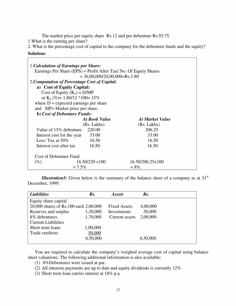
The market price per equity share Rs.12 and per debenture Rs.93.75.
1.What is the earning per share?
2. What is the percentage cost of capital to the company for the debenture funds and the equity?
Solution:
1.Calculation of Earnings per Share:
Earnings Per Share (EPS) = Profit After Tax/ No. Of Equity Shares
= 36,00,000/20,00,000=Rs.1.80
2.Computation of Percentage Cost of Capital.
a) Cost of Equity Capital:
Cost of Equity (Ke) = D/MP
or Ke (%)= 1.80/12 *100= 15%
where D = expected earnings per share
and MP= Market price per share.
b) Cost of Debenture Funds:
At Book Value At Market Value
(Rs. Lakhs) (Rs. Lakhs)
Value of 15% debenture 220.00 206.25
Interest cost for the year 33.00 33.00
Less: Tax at 50% 16.50 16.50
Interest cost after tax 16.50 16.50
Cost of Debenture Fund
(%) 16.50/220 x100 16.50/206.25x100
= 7.5% = 8%.
Illustration5: Given below is the summary of the balance sheet of a company as at 31st
December, 1999:
Liabilities Rs. Assets Rs.
Equity share capital
20,000 shares of Rs.100 each 2,00,000 Fixed Assets 4,00,000
Reserves and surplus 1,30,000 Investments 50,000
8% debentures 1,70,000 Current assets 2,00,000
Current Liabilities
Short term loans 1,00,000
Trade creditors 50,000
6,50,000 6,50,000
You are required to calculate the company’s weighed average cost of capital using balance
sheet valuations: The following additional information is also available:
(1) 8%Debentures were issued at par.
(2) All interests payments are up to date and equity dividends is currently 12%.
(3) Short term loan carries interest at 18% p.a

18
(4) The shares and debentures of the company are all quoted on the Stock Exchange and
current Market prices are as follows:
Equity Shares Rs.14 each
8% Debentures Rs.98 each.
(5) The rate of tax for the company may be taken at 50%.
Solution:
Calculation of the Cost of Equity: Rs.
Equity Share 2,00,000
Reserves and Surplus 1,30,000
Equity (Shareholder’s )Fund 3,30,000
Book Value Per Share = 3,30,000/20,000 =Rs.16.50.
Equity Dividend Per Share = 12/100*10 =Rs.1.20
Therefore, Cost Of Equity (%)= 1.20/16.50*100= 7.273 %
Computation of Weighted Average Cost of Capital:
Capital Structure or
Type of Capital Amount (Rs) Before Tax After Tax Weighted Average
cost Cost% (Rs.) Cost%
Equity Funds 3,30,000 7.273% 7.273% 24,000
Debentures 1,70,000 8% 4% 6,800
Total 5,00,000 30,800
Weighted Average Cost of Capital = 30,800/5,00,000*100 =6.16 %.

19
Summary of Formulae
S.No
Purpose Formula
1
2
3
4
5
6
7
8
9
10
11
12
13
Before tax cost of debt
After cost of debt
Before tax cost of redeemable debt
After tax cost of redeemable debt
Cost of debt redeemable at premium
Cost of debt redeemable in instalments
Cost of irredeemable preference share capital
Cost of redeemable preference share capital
Cost of equity –dividend yield approach
Cost of equity – dividend yield plus constant
growth
Cost of retained earnings
Weighted average cost of capital
Cost of equity – CAPM approach
Kdb =NP
I
Kda = Kdb (1-t) = ( )tNP
I−1
( )
( )NPP
NPPn
I
Kdb
+
−+
=
2
1
1
Kda = Kdb (1-t)
( )
( )NPRV
NPRVn
I
Kdb
+
−+
=
2
1
1
Vd = ( )
∑− +
+n
t
t
d
tt
KI
PI
1
Kp = NP
D
( )NPMV
n
NPMVD
Kpr
+
−+
=
2
1
Ke = MP
Dor
NP
D
Ke = ( )
GNP
gDG
NP
DO +
+=+
11
Kr = GNP
D+
Kw = W
XW
∑
∑
Ke = Rf + β I (Rm - Rf )

20
Lets Sum Up
� The cost of capital is the minimum required rate of return which firm must earn on its
funds in order to satisfy the expectation of its supplier of funds. If the return from capital
budgeting proposals is more than cost of capital then difference will be added to wealth
of shareholders.
� The concept of cot of capital has a role to play in capital budgeting as well as in finalizing
the capital structure for the firm. The cost of capital depends upon the risk free interest
rate and risk premium, which depends upon the risk of investment and risk of firm.
� The cost of capital may be defined in terms of (1) explicit cost, which the firm pays to
supplier, and (2) implicit cost. i.e. opportunity cost of funds to firm. The cost of capital is
calculated in after tax terms.
� Different sources of funds available to firm may be grouped into Debt, Pref. share capital,
Equity share capital and retained earning and these sources have their specific cost of
capital. However the overall cost of capital of the firm may be ascertained as the
weighted average of these specific costs of capital.
� The cost of retained earnings is lower than cost of equity as former does not have any
floatation cost.
� The Weighted average cost of capital WACC may be ascertained by applying book value
weights or market value weights of different sources of funds. The WACC is denoted as
Kw.
QUESTIONS
1. What is the relevance and significance of cost of capital in capital budgeting? How does the
cost of capital enter the capital budgeting process?
2. Define the concept of cost of capital? State how you would determine the weighted average
cost of capital of a firm?
3. How cost of equity capital is determined under CAPM?
4. Write short notes on (a) Marginal cost of capital (b) Cost of retained earnings
5. The cost of preference capital is generally lower than cost of equity. State the reasons?
6. What are the problems in determining the cost of capital?
7. How is the cost of zero coupon bonds determined?

21
3
CAPITAL STRUCTURE THEORIES
Smriti Chawla Shri Ram College of Commerce
University of Delhi
Concept of Capital Structure
Capital Structure refers to the proportionate amount that makes up capitalisation. Some
authors include retained earnings and capital surplus for the purpose of capital structure; in that
case capital structure shall be:
Rs. Proportion/Mix
Equity Share Capital 10,00,000 42.55%
Preference Share Capital 5,00,000 21.28%
Long-Term loans and Debentures 2,00,000 8.51%
Retained Earnings 6,00,000 25.53%
Capital Surplus 50,000 2.13%
23,50,000 100%
Hence, the term capital structure refers to the firm’s permanent or long term financing
consisting of equity share capital, retained earnings, preference share capital, debentures and
long-term debts.
CHAPTER OBJECTIVES
� Concept of Capital Structure � Optimal Capital Structure � Objects of Appropriate Capital Structure � Importance of Capital Structure � Theories of Capital Structure
o Net Income Approach o Net Operating Income Approach o Traditional Approach
o Modigliani and Miller Model

22
Optimal Capital Structure
The capital structure decision can influence the value of the firm through the cost of
capital and trading on equity or leverage. The optimum capital structure may be defined as “that
capital structure or combination of debt and equity that leads to the maximum value of the firm”
optimal capital structure ‘maximum’ the value of the company and hence the wealth of its
owners and minimizes the company’s cost of capital’ (Solomon, Ezra, the Theory of Financial
Management). Thus every firm should aim at achieving the optimal capital structure and then to
maintain it.
The following considerations should be kept in mind while maximizing the value of the
firm in achieving the goal of optimum capital structure:
(i) If the return on investment is higher than the fixed cost of funds, the company should
prefer to raise funds having a fixed cost, such as debentures, loans and preference share
capital. It will increase earnings per share and market value of the firm. Thus, a company
should, make maximum possible use of leverage.
(ii) When debt is used as source of finance, the firm saves a considerable amount in payment
of tax as interest is allowed a deductible expense in computation of tax. Hence, the
effective cost of debt is reduced called tax leverage. A company should, therefore, take
advantage of tax leverage.
(iii) The firm should undue financial risk attached with the use of increased debt financing. It
the shareholders perceive high risk in using further debt-capital, it will reduce the market
price of shares.
(iv) The capital structure should be flexible.
Objects of an Appropriate Capital Structure
The objects of an appropriate capital structure have been summarized by Soloman Ezra in
the following words:
“The advantage of having an appropriate financial structure, if such an optimum does
exist, are two fold, it maximizes value of the company and hence the wealth of its owner; it
minimizes the company’s cost of capital which in turn increases its ability to find new wealth
creating investment opportunities. Also by increasing the firm’s opportunities to engage in future
wealth creating investment, it increases the economy’s rate of investment and growth.”
More specifically, the objects may be classified as follows:
� Minimisation of cost of capital
� Minimization of Risk
� Maximization of Return
� Preservation of control
Importance of Capital Structure
The term 'Capital structure' refers to the relationship between the various long-term forms
of financing such as debenture, preference share capital and equity share capital. Financing the
firm's assets is a very crucial problem in every business and as a general rule there should be a
proper mix of debt and equity capital in financing the firm’s assets. The use of long –term fixed
23
interest bearing debt and preference share capital along with equity shares is called financial
leverage or trading on equity. The long-term fixed interest bearing debt is employed by a firm to
earn more from the use of these sources than their cost so as to increase the return on owner’s
equity. It is true the capital structure cannot affect the total earnings of a firm but it can affect the
share of earnings available for equity shareholders. Say, for example a company has an equity
capital of 1000 shares of Rs. 100 each fully paid and earns an average profits of Rs. 30,000. Now
the company wants to make an expansion and needs another of Rs. 1,00,000.The options with
the company are-either to issue new shares or raise loans @ 10% p.a. Assuming that the
company would earn the same rate of profits. It is advisable to raise loans a by doing so earnings
per share will magnify. The company shall pay only Rs. 10,000 as interest and profit expected
shall be Rs. 60,000 (before payment of interest). After the payment of interest the profits left for
equity shareholders shall be Rs. 50,000 (ignoring tax). It is 50% return on the equity capital
against 30% return otherwise. However, leverage can operate adversely also if the rate the
interest on long-terms loans is more than the expected rate of earnings of the firm.
The impact of leverage on earnings per share (EPS) can be understood with the help of
following illustration.
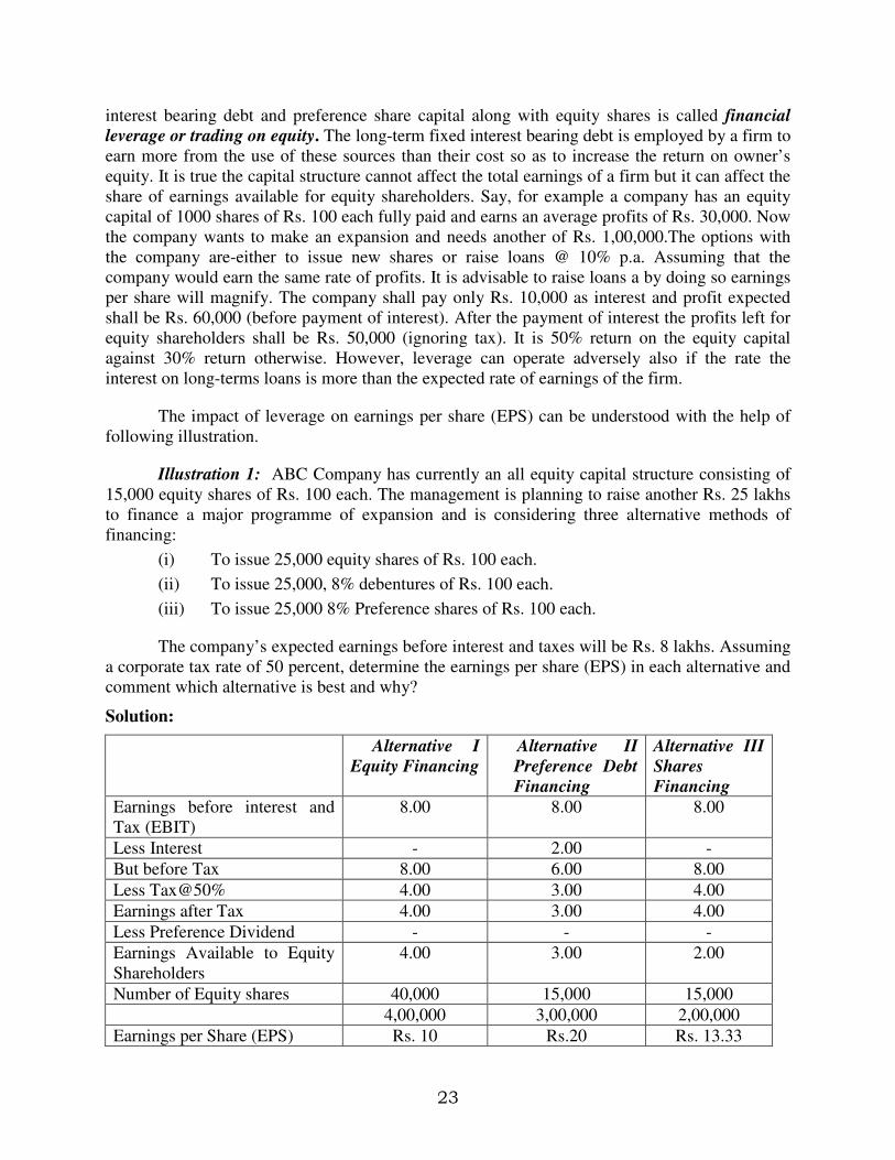
Illustration 1: ABC Company has currently an all equity capital structure consisting of
15,000 equity shares of Rs. 100 each. The management is planning to raise another Rs. 25 lakhs
to finance a major programme of expansion and is considering three alternative methods of
financing:
(i) To issue 25,000 equity shares of Rs. 100 each.
(ii) To issue 25,000, 8% debentures of Rs. 100 each.
(iii) To issue 25,000 8% Preference shares of Rs. 100 each.
The company’s expected earnings before interest and taxes will be Rs. 8 lakhs. Assuming
a corporate tax rate of 50 percent, determine the earnings per share (EPS) in each alternative and
comment which alternative is best and why?
Solution:
Alternative I
Equity Financing
Alternative II
Preference Debt
Financing
Alternative III
Shares
Financing
Earnings before interest and
Tax (EBIT)
8.00 8.00 8.00
Less Interest - 2.00 -
But before Tax 8.00 6.00 8.00
Less Tax@50% 4.00 3.00 4.00
Earnings after Tax 4.00 3.00 4.00
Less Preference Dividend - - -
Earnings Available to Equity
Shareholders
4.00 3.00 2.00
Number of Equity shares 40,000 15,000 15,000
4,00,000 3,00,000 2,00,000
Earnings per Share (EPS) Rs. 10 Rs.20 Rs. 13.33

24
Comments: As the earnings per share highest in alternative II, i.e. debt financing, the
company should issue 25,000 8% debentures of Rs. 100 each. It will double the earnings of the
equity shareholders without loss of any control over the company.
Theories of Capital Structure
Different of theories have been propounded by different authors to explain the
relationship between capital structure, cost of capital and value of the firm. The main
contributors to the theories are Durand, Ezra, Solomon, Modigliani and Miller. The important
theories are discussed below:
1. Net Income Approach.
2. Net Operating Income Approach.
3. The Traditional Approach
4. Modigliani and Miller Approach.
Assumptions: For clear understanding of the theories of capital structure and relationship
between capital structure, cost of capital and the value of firm, following assumptions are
made:
� The firm uses only two sources of funds i.e debt and equity
� The firm’s total assets are given and its investment decisions do not change.
� The firm’s total financing remains unchanged but degree of leverage can be changed for
replacing debt for equity or equity for debt.
� The firm’s dividend pay out ratio is 100% and it does not a all retain the earnings.
� The EBIT is not expected to grow.
� Business risk of the firm is constant and it is assumed to be independent of capital
structure and financial risk.
� Investor’s subjective probability distribution of the future expected operating earnings of
the firm is the same.
(1) Net Income Approach
According to this approach, a firm can minimize the weighted average cost of capital and
increase the value of the firm as well as market price of equity shares by using debt financing
to the maximum possible extent. The theory propounds that a company can increase its value
and reduce the overall cost of capital by increasing the proportion of debt in its capital
structure. This approach is based upon the following assumptions:
(i) The cost of debt is less than the cost of equity.
(ii) There are no taxes.
(iii) The risk perception of inventors is not changed by the use of debt.

25
The line of argument in favour of net income approach is that as proportion of debt
financing in capital structure increase¸ the proportion of and cheaper source of funds increases.
This result in the decrease in overall (weighted average) cost of capital leading to an increase in
the value of the firm. The reasons for assuming cost of debt to be less than the cost of equity are
that interest rates are usually lower than dividend rates due to element of risk and the benefit of
tax as the interest is a deductible expense.
The figure shows that kd and ke are constant for all levels of leverages i.e. for all levels of
debt financing. As the debt proportion of the financial leverage increases, the WACC, ko,
decreases as the kd is less than ke. This result in the increase in value of the firm. It may be noted
that ko will approach kd as the debt proportion is increased. However, ko will never touch kd as
there cannot be a 100% debt firm. Some element of equity must be there. However, if the firm is
100% equity firm, then the ko is equal to ke. The rate of decline in ko depends upon the relative
position of kd and ke. Net Income Approach suggests that higher the degree of leverage, better it
is, as the value of the firm would be higher.
Illustration 2: (a) A company expects a net income of Rs. 80,000. It has Rs. 2,00,000,
8% Debentures. The equity capitalization rate of the company is 10%. Calculate the value of the
firm and overall capitalisation rate according to the Net Income Approach (ignoring income-tax).
(b) If the debenture debt is increased to Rs. 3,00,000, what shall be the value of the firm and the
overall capitalisation rate?

26
Solution:
(a) Calculation Of The Value Of The Firm
Market Value of Equity = 64, 000× 10
100
= Rs. 6,40,000
Market Value of Debentures = Rs. 2,00,000
Value of the Firm = Rs. 8,40,000
Calculation Of Overall Capitalisation Rate
Overall Cost of Capital (ko) =
V
EBIT
firmtheofValue
Earningsx
= 100x000,40,8
000,80
= 9.52%
b) Calculation Of Value Of The Firm If Debenture Debits Raised To Rs. 3,00,000
Rs
Net Income 80,000
Less: Interest on 8% Debentures of Rs. 3,00,000 24,000
Earnings available to equity shareholders 56,000
Equity Capitalisation Rate 10% 10%
Market Value of Equity = 56,000× 10
100
= Rs. 5,60,000
Market Value of Debentures = Rs. 3,00,000
Value of the Firm = Rs. 8,60,000
Overall Capitalisation Rate = 000,60,8
000,80× 100 = 9.30%

27
Thus, it is evident that with the increase in debt financing the value of the firm has increased and
the overall cost of capital has decreased.
( 2 ) Net Operating Income Approach
This theory as suggested Durand is another extreme of the effect of leverage on the value
of the firm. It is diametrically opposite to the net income approach. According to this approach,
change in the capital structure of a company does not affect the market value of the firm and the
overall cost of capital remains constant irrespective of the method of financing. It implies that the
overall of capital remains the same whether the debt-equity mix is 50:50 or 20:80 or 0:100.
Thus, there is nothing as an optimal capital structure and every capital structure is the optimum
capital structure. This theory presumes that:
(i) the market capitalizes the value of the firm as a whole;
(ii) the business risk remains constant at every level of debt equity mix.
The reasons propounded for such assumptions are that the increased use of debt increase
the financial risk of the equity shareholders and hence the cost of equity increases. On the other
hand, the cost of debt remains constant with the increasing proportion of debt as the financial
risk of the lenders is not affected. Thus, the advantage of using the cheaper source of funds, i.e.;
debt is exactly offset by the increased cost of equity.
The figure shows that the cost of debt, kd, and the overall cost of capital, ko, are constant
for all levels of leverage. As the debt proportion or the financial leverage increases, the risk of
the shareholders also increases and thus the cost of equity capital, ke also increases. However, the
increase in ke, is such that the overall value of the firm remains same. It may be noted that for an
all equity firm, the ke is just equal to ko. As the debt proportion is increased, the ke also increases.
However, the overall cost of capital remains constant because increase in ke is just sufficient to
off set the benefits of cheaper debt financing.

28
Illustration 3 (a): A company expected a net operating income of Rs. 1,00,000. It has Rs.
5,00,000, 6% Debentures. The overall capitalisation rate is 10%. Calculate the value of the firm
and the equity capitalisation rate (cost of equity) according to the Net Operating Income
Approach.
(b) If the debenture debt is increased to Rs. 7,50,000. what will be the effect on the value of the
firm and the equity capitalisation rate?
Solution:
(a) Net Operating Income = Rs. 1,00,000
Overall Cost of Capital = 10%
Market Value of the first (V) = )(0K
EBIT
CapitalofCostOverall
comeOpeartingnNet
= 1,00,000× 10
100
= Rs. 10,00,000
Market Value of Firm Rs. 10,00,000
Less: Market Value of Debentures Rs. 5,00,000
Total Market Value of Equity Rs. 5,00,000
Equity Capitalisation Rate or Cost of equity (Ke)
= Earnings available to equity shareholders or EBIT – I/V - B
Total market value of equity shares
(where, EBIT means Earnings before Interest and Tax)
V is Value of the firm
B is Value of debt capital
I is interest on debt
= 1,00,000 – 30,000/10,00,000 – 5,00,000 × 100
=
000,00,5
000,70×100=14%
(b) If the debenture debt is increased to Rs. 7,50,000, the value of the firm shall remain
unchanged at Rs. 10,00,000. The equity capitalisation rate will increase as follows:

29
Equity Capitalization Rate (ke)
= EBIT – I / V - B
= 1,00,000 – 45,000/10,00,000 – 7,50,000×100
= 000,50,2
000,55×100 = 22%
(3) The Traditional Approach
The traditional approach, also known as Intermediate approach, is a compromise between
the two extremes of net income approach and net operating income approach. According to this
theory, the value of the firm can be increased initially or the cost of capital can be decreased by
using more debt as the debt is a cheaper source of funds than equity. Thus, optimum capital
structure can be reached by a proper debt-equity mix. Beyond a particular point, the cost of
equity increases because increase debt increases the financial risk of the equity shareholders. The
advantage of cheaper debt at this point of capital structure is offset by increased cost of equity
after this there comes a stage, when the increased cost of equity cannot be offset by the
advantage of low-cost debt. Thus, overall cost of capital, according to this theory, decreases upto
a certain point, remains more or less unchanged for moderate increase in debt thereafter: and
increase or rises beyond a certain point. Even the cost of debt may increase at this state due to
increased financial risk.
Traditional View point on the relationship between Leverage, cost of
capital and value of the firm.
The figure shows that there can either be a particular financial leverage (as in Part A) or a
range of financial leverage (as in Part B) when the overall cost of capital, ko is minimum. The
figure in Part A shows that at the financial leverage level O, the firm has the lowest ko and
therefore, the capital structure at that financial leverage is optimal. The Part B of the figure
shows that there is not one optimal capital structure, rather there is a range of optimal capital
structure from leverage level O to level P. Every capital structure over this range of financial
leverage is an optimal capital structure. Thus, as per the traditional approach, a firm can be
benefited from a moderate level of leverage when the advantages using debt (having lower cost)
out weigh the disadvantages of increasing ke (as a result of higher financial risk). The overall
cost of capital, ko, therefore is a function of the financial leverage. The value of the firm can be
affected therefore, by the judicious use of debt and equity in the capital structure.

30
Illustration 4: Compute the market value of the firm, value of shares and the average cost of
capital from the following information:
Rs.
Net Operating Income 2,00,000
Total Investment 10,00,000
Equity Capitalisation Rate:
a) If the firm uses no debt 10%
b) If the firm uses Rs. 4,00,000 debentures 11%
c) If the firm uses Rs. 6,00,000 debentures 13%
Assume that Rs.4,00,000 debentures can be raised at 5% rate of interest whereas Rs. 6,00,000
debentures can be raised at 6% rate of interest.
Solution:
Computation of Market Value of Firm, Value of Shares & the Average Cost of Capital
(a) No debt (b)Rs.4,00,000
5%Debentures
(c)Rs.6,00,000
6%Debentures
Net Operating Income Rs. 2,00,000 Rs. 2,00,000 Rs. 2,00,000
Less: Interest i.e., Cost of
debt:
20,000
36,000
Earnings available to
Equity Shareholders
Rs. 2,00,000 Rs.1,80,000 Rs. 1,64,000
Equity Capitalisation Rate 10% 11% 13%
Market Value of shares 2,00,000×
10
100 1,80,000×
11
100 1,64,000×
13
100
Rs. 20,00,000 Rs. 16,36,363 Rs. 12,61,538
Market value of debt
(debentures)
Market Value of firm
20,00,000
4,00,000
20,36,363
6,00,000
18,61,538
Average Cost of Capital
000,00,20
000,00,2×100
363,36,20
000,00,2×100
538,61,18
000,00,2×100
V
EBITor
firmtheofValue
Earnings
= 10% = 9.8% = 10.7%
Comments: It is clear from the above that if debt of Rs. 4,00,000 is used the value of the firm
increases and the overall cost of capital decreases. But, if more debt is used to finance in place of
equity, i.e., Rs. 6,00,000 debentures, the value of the firm decreases and the overall cost of
capital increases.
31
(4) Modigliani-Miller Approach
M&M hypothesis is identical with the Net Operating Income approach if taxes are
ignored. However, when corporate taxes are assumed to exist, their hypothesis is similar to the
Net Income Approach.
(a) In the absence of taxes: The theory proves that the cost of capital is not affected by
changes in the capital structure or say that the debt-equity mix is irrelevant in the determination
of the total value of a firm. The reason argued is that though debt is cheaper to equity, with
increased use of debt as a source of finance, the cost of equity increases. This increases in cost of
equity offsets the advantages of low cost of debt. Thus, although the financial leverage affects
the cost of equity, the overall cost of capital remains constant. The theory emphasizes the fact
that firm’s operating income is a determinant of its total value. The theory further propounds that
beyond a certain limit of debt, the cost of debt increases (due to increased financial risk) but the
cost of equity falls thereby again balancing the two costs. In the opinion of Modigliani & Miller,
two identical firms in all respects except their capital structure cannot have different market
values or cost of capital because of arbitrage process. In case two identical firms except for their
capital structure have different market values or cost of capital arbitrage will take place and the
investors will engage in ‘personal leverage’ (i.e. they will buy equity of the other company in
preference to the company having lesser value) as against the corporate leverage’: and this will
again render the two firms to have the same total value.
The M&M approach is based upon the following assumptions:
(i) There are no corporate taxes.
(ii) There is a perfect market.
(iii) Investors act rationally.
(iv) The expected earnings of all the firms have identical risk characteristics.
(v) The cut-off point of investment in a firm is capitalization rate.
(vi) Risk to investors depends upon the random fluctuations of expected earnings and
the possibility that the actual value of the variables may turn out to be different
from best estimates.
(vii) All earnings are distributed to the shareholders.
(b) When the corporate taxes are assumed to exist: Modigliani and Miller, in their
article of 1963 have recognized that the value of the firm will increase or the cost of capital will
decrease with the use of debt on account of deductibility of interest charges for tax purpose.
Thus, the optimum capital structure can be achieved by maximizing the debt mix in the equity of
a firm.
According to the M&M approach, the value of a firm unlevered can be calculated as.
Value of unlevered firm (Vu)
= Earnings before interest and tax/Overall cost of capital
= EBIT/ko (1 – t)
and, the value of a levered firms is:
VL=Vu+tD
32
where, Vu is value of unlevered firm
and, tD is the discounted present value of the tax savings resulting from the tax deductibility of
the interest charges, t is the rate of tax and D the quantum of debt used in the mix.
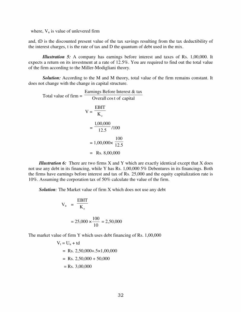
Illustration 5: A company has earnings before interest and taxes of Rs. 1,00,000. It
expects a return on its investment at a rate of 12.5%. You are required to find out the total value
of the firm according to the Miller-Modigliani theory.
Solution: According to the M and M theory, total value of the firm remains constant. It
does not change with the change in capital structure.
Total value of firm = capitaloftcosOverall
tax&InterestBeforeEarnings
V =oK
EBIT
= 5.12
000,00,1/100
= 1,00,000× 5.12
100
= Rs. 8,00,000
Illustration 6: There are two firms X and Y which are exactly identical except that X does
not use any debt in its financing, while Y has Rs. 1,00,000 5% Debentures in its financings. Both
the firms have earnings before interest and tax of Rs. 25,000 and the equity capitalization rate is
10%. Assuming the corporation tax of 50% calculate the value of the firm.
Solution: The Market value of firm X which does not use any debt
Vu = oK
EBIT
= 25,000 ×10
100 = 2,50,000
The market value of firm Y which uses debt financing of Rs. 1,00,000
Vt = Uu + td
= Rs. 2,50,000+.5×1,00,000
= Rs. 2,50,000 + 50,000
= Rs. 3,00,000

33
How does the Arbitrage Process Work?
We have noticed in illustration that the market value of firm Y, which uses debt content
in its capital structure, is higher than the market value of firm X which does not use debt content
in its capital structure. According to M & M theory, this situation cannot remain for a long
period because of the arbitrage process. As the investors in company Y can earn a higher rate of
return on their investment with lower financial risk, they will sell their holding of shares in
company X and invest the same in company Y. Further, as company Y does not use any debt in
its capital structure the financial risk to the investors will be less, thus, they will engage in
personal leverage by borrowing additional funds equivalent to their proportionate share in firm
X’s debt at the same rate of interest and invest the borrowed funds also in company Y. The
arbitrage process will continue till the prices of shares of company X fall and that of company Y
rise so as to make the market value of the two funds identical However, in the arbitrage process,
such investors who switch their holdings will gain. Illustration, given below, illustrates the
working of arbitrage process.
Illustration 7: The following is the data regarding two companies ‘A’ and ‘B’ belonging to the
same equivalent risk class:
Company A Company B
Number of ordinary shares 1,00,000 1,50,000
8% Debentures 50,000 _
Market Price per share Rs. 1.30 Rs. 1.00
Profit before interest Rs. 20,000 Rs. 20,000
All profits after paying debenture interest are distributed as dividends. You are required to
explain how under Modigliani and Miller approach, an investor holding 10% of shares in
company ‘A’ will be better off in switching his holding to company ‘B’
Solution: In the opinion of Modigliani & Miller, two identical firms in all respects except their
capital structure cannot have different market values because of arbitrage process. In case two
identical firms except for their capital structure have different market values, arbitrage will take
place and the investors will engage in ‘personal leverage’ as against the corporate leverage. In
the given problem, the arbitrage will work out as below:
1. The investor will sell in the market 10% of shares in company ‘A’ for Rs. 13,000
(100
10×1,00,000×1.30)
2. He will raise a loan of Rs. 5000 (100
10×50,000) to take advantage of personal leverage
as against the corporate leverage as company ‘B’ does not use debt content in its
capital structure.
3. He will buy 18,000 shares in company ‘B’ with the total amount realised from 1 and
2, i.e., Rs. 13,00 plus Rs. 5000, Thus he will have 12% of shares in company ‘B’.

34
The investor will gain by switching his holding as below:
Present income of the investor in company ‘A’:
Profit before interest of the company = Rs. 20,000
Less Interest on debentures (8%) = Rs. 4,000
Profit after Interest 16,000
Share of the investor = 10% of Rs. 16,000 i.e. Rs. 1600
Income of the investor after switching holding to company ‘B’
Profit before interest for company ‘B’ = Rs. 20,000
Less Interest = Nil
Profit after interest 20,000
Share of the investor = 20,000 × 000,50,1
000,18 = Rs. 2400
Less: Interest paid on loan taken 8% of Rs. 5000 = 400
Net Income of the investor 2000
As the net income of the investor in company ‘B’ is higher than the loss of income from
company ‘A’ due to switching the holding, the investor will gain in switching his holding to
company ‘B’.

35
4
CAPITAL STRUCTURE: PLANNING AND DESIGNING
Smriti Chawla
Shri Ram College of Commerce University of Delhi
Capital Structure Management or Planning The Capital Structure
Estimation of capital requirements for current and future needs is important for a firm.
Equally important is the determining of capital mix. Equity and debt are the two principle
sources of finance of a business. But, what should be the proportion between debt and equity in
the capital structure of a firm now much financial leverage should a firm employ? This is a very
difficult question. To answer this question, the relationship between the financial leverage and
the value of the firm or cost of capital has to be studied. Capital structure planning, which aims at
the maximisation of profits and the wealth of the shareholders, ensures the maximum value of a
firm or the minimum cost of the shareholders. It is very important for the financial manager to
determine the proper mix of debt and equity for his firm. In principle every firm aims at
achieving the optimal capital structure but in practice it is very difficult to design the optimal
capital structure. The management of a firm should try to reach as near as possible of the
optimum point of debt and equity mix.
Essential Features of a Sound Capital Mix
A sound or an appropriate capital structure should have the following essential features:
(i) Maximum possible use of leverage.
CHAPTER OBJECTIVES
� Capital Structure Management or planning the Capital Structure
� Essential features of sound capital mix
� Factors determining capital structure � Profitability and Capital Structure: EBIT
– EPS Analysis � Liquidity and Capital Structure: Cash
Flow Analysis
� Illustrations � Lets Sum Up
� Questions

36
(ii) The capital structure should be flexible.
(iii) To avoid undue financial/business risk with the increase of debt.
(iv) The use of debt should be within the capacity of a firm. The firm should be in a
position to meet its obligation in paying the loan and interest charges as and when
due.
(v) It should involve minimum possible risk of loss of control.
(vi) It must avoid undue restrictions in agreement of debt.
(vii) The capital structure should be conservative. It should be composed of high grade
securities and debt capacity of the company should never be exceeded.
(viii) The capital structure should be simple in the sense that can be easily managed and
also easily understood by the investors.
(ix) The debt should be used to the extent that it does not threaten the solvency of the
firm.
Factors Determining the Capital Structure
The capital structure of a concern depends upon a large number of factors such as
leverage or trading on equity, growth of the company, nature and size of business, the idea of
retaining control, flexibility of capital structure, requirements of investors costs of floatation of
new securities, timing of issue, corporate tax rate and the legal requirements. It is not possible to
rank them because all such factors are of different importance and the influence of individual
factors of a firm changes over a period of time. Every time the funds are needed. The financial
manager has to advantageous capital structure. The factors influencing the capital structure are
discussed as follows:
1. Financial leverage of Trading on Equity: The use of long term fixed interest bearing
debt and preference share capital along with equity share capital is called financial
leverage or trading on equity. The use of long-term debt increases, magnifies the earnings
per share if the firm yields a return higher than the cost of debt. The earnings per share
also increase with the use of preference share capital but due to the fact that interest is
allowed to be deducted while computing tax, the leverage impact of debt is much more.
However, leverage can operate adversely also if the rate of interest on long-term loan is
more than the expected rate of earnings of the firm. Therefore, it needs caution to plan the
capital structure of a firm.
2. Growth and stability of sales: The capital structure of a firm is highly influenced by the
growth and stability of its sale. If the sales of a firm are expected to remain fairly stable,
it can raise a higher level of debt. Stability of sales ensures that the firm will not face any
difficulty in meeting its fixed commitments of interest repayments of debt. Similarly, the
rate of the growth in sales also affects the capital structure decision. Usually greater the
rate of growth of sales, greater can be the use of debt in the financing of firm. On the

37
other hand, if the sales of a firm are highly fluctuating or declining, it should not employ,
as far as possible, debt financing in its capital structure.
3. Cost of Capital. Every rupee invested in a firm has a cost. Cost of capital refers to the
minimum return expected by its suppliers. The capital structure should provide for the
minimum cost of capital. The main sources of finance for a firm are equity, preference
share capital and debt capital. The return expected by the suppliers of capital depends
upon the risk they have to undertake. Usually, debt is a cheaper source of finance
compared to preference and equity capital due to (i) fixed rate of interest on
debt: (ii) legal obligation to pay interest: (iii) repayment of loan and priority in payment
at the time of winding up of the company. On the other hand, the rate of dividend is not
fixed on equity capital. It is not a legal obligation to pay dividend and the equity
shareholders undertake the highest risk and they cannot be paid back except at the
winding up of the company and that too after paying all other obligations. Preference
capital is also cheaper than equity because of lesser risk involved and a fixed rate of
dividend payable to preference shareholders. But debt is still a cheaper source of finance
than even preference capital because of tax advantage due to deductibility of interest.
While formulating a capital structure, an effort must be made to minimize the overall cost
of capital.
4. Minimisation of Risk: A firm’s capital structure must be developed with an eye towards
risk because it has a direct link with the value. Risk may be factored for two
considerations: (a) the capital structure must be consistent with the business risk,
and (b) the capital structure results in certain level of financial risk. Business risk may be
defined as the relationship between the firm's sales and its earnings before interest and
taxes (EBIT). In general, the greater the firm's operating leverage – the use of fixed
operating cost – the higher its business risk. Although operating leverage is an important
factor affecting business risk, two other factors also affect it – revenue stability and cost
stability. Revenue stability refers to the relative variability of the firm's sales revenue.
Firms with highly volatile product demand and price have unstable revenues that result in
high levels of business risk. Cost stability is concerned with the relative predictability of
input price. The more predictable and stable these inputs prices are, the lower is the
business risk, and vice-versa. The firm's capital structure directly affects its financial risk,
which may be described as the risk resulting from the use of financial leverage. Financial
leverage is concerned with the relationship between earnings before interest and taxes
(EBIT) and earnings per share (EPS). The more fixed-cost financing i.e., debt (including
financial leases) and preferred stock, a firm has in capital structure, the greater its
financial risk.
5. Control: The determination of capital structure is also governed by the management
desire to retain controlling hands in the company. The issue of equity share involve the
risk of losing control. Thus in case the company is interested in – retaining control, it
should prefer the use of debt and preference share capital to equity share capital.
However, excessive use of debt and preference capital may lead to loss of control and
other bad consequences.

38
6. Flexibility: The term flexibility refers to the firm’s ability to adjust its capital structure to
the requirements of changing conditions. A firm having flexible capital structure would
face no difficulty in changing its capitalization or source of fund. The degree of
flexibility in capitals structure depends mainly on (i) firm’s unused debt capacity,
(ii) terms of redemption (iii) flexibility in fixed charges, and (iv) restrictive stipulation in
loan agreements.
If a company has some unused debt capacity, it can raise funds to meet the sudden
requirements of finances. Moreover, when the firm has a right to redeem debt and preference
capital at its discretion it will able to substitute the source of finance for another, whenever
justified. In essence, a balanced mix of debt and equity needs to be obtained, keeping in view
the consideration of burden of fixed charges as well as the benefits of leverages
simultaneously.
7. Profitability: A capital structure should be the most profitable from the point of view of
equity shareholders. Therefore, within the given constraints, maximum debt financing
(which is generally cheaper) should be opted to increase the returns available to the
equity shareholder.
8. Cash Flow Ability: The EBIT – EPS analysis, growth of earnings and coverage ratio are
very useful indicator of a firm’s ability to meet its fixed obligations at various levels of
EBIT. Therefore, an important feature of a sound capital structure is the firm’s ability to
generate cash flow to service fixed charges.
At the time of planning the capital structure, the ratio of net cash inflows to fixed charges
should be examined. The ratio depicts the number of times the fixed charges commitments
are covered by net cash inflows. Greater is this coverage, greater is this capacity of a firm to
use debts an other sources of funds carrying fixed rate of interest and dividend.
9. Characteristics of the company: The peculiar characteristics of a company in regards to
its size, nature, credit standing etc. play a pivotal role in ascertaining its capital structure.
A small size company will not be able to raise long-term debts at reasonable rate of
interest on convenient terms. Therefore, such companies rely to a significant extent on
the equity share capital and reserves and surplus for their long-term financial
requirements.
In case of large companies the funds can be obtained on easy terms and reasonable cost by
selling equity shares and debentures as well. Moreover the risk of loss of control is also less in
case of large companies, because their shares can be distributed in a wider range. When company
is widely held, the dissident shareholders will not be able to organize themselves against the
existing management, hence, no risk of loss of loss of control. Thus, size of a company has a
vital role to play in determining the capital structure.
The various elements concerning variation in sales, competition with other firms and life
cycle of industry also affect the form and size of capitals structure. If company’s sales are subject
to wide fluctuations, it should rely less on debt capital and opt for conservative capitals structure.
A company facing keen competition with other companies will run the excessive risk of not

39
being able to meet payments on borrowed funds. Such companies should place much emphasis
on the use of equity than debt, similarly, if a company is in infancy stage of its life cycle, it will
run a high risk of mortality. Therefore, companies in their infancy should rely more on equity
than debt. As a company grows mature, it can make use of senior securities (bonds and
debentures).
Capital Structure of a New Firm : The capital structure a new firm is designed in the initial
stages of the firm and the financial manager has to take care of many considerations. He is
required to assess and evaluate not only the present requirement of capital funds but also the
future requirements. The present capital structure should be designed in the light of a future
target capital structure. Future expansion plans, growth and diversifications strategies should be
considered and factored in the analysis.
Capital Structure of an Existing Firm: An existing firm may require additional capital funds
for meeting the requirements of growth, expansion, diversification or even sometimes for
working capital requirements. Every time the additional funds are required, the firm has to
evaluate various available sources of funds vis-à-vis the existing capital structure. The decision
for a particular source of funds is to be taken in the totality of capital structure i.e., in the light of
the resultant capital structure after the proposed issue of capital or debt.
Evaluation of Proposed Capital Structure : A financial manager has to critically evaluate
various costs and benefits, implications and the after-effects of a capital structure before deciding
the capital mix. Moreover, the prevailing market conditions are also to be analyzed. For example,
the present capital structure may provide a scope for debt financing but either the capital market
conditions may not be conducive or the investors may not be willing to take up the debt-
instrument. Thus, a capital structure before being finally decided must be considered in the light
of the firm’s internal factors as well as the investor's perceptions.
Profitability and Capital Structure: EBIT – EPS Analysis
The financial leverage affects the pattern of distribution of operating profit among
various types of investors and increases the variability of the EPS of the firm. Therefore, in
search for an appropriate capitals structure for a firm, the financial manager must analysis the
effects of various alternative financial leverages on the EPS. Given a level of EBIT, EPS will be
different under different financing mix depending upon the extent of debt financing. The effect
of leverage on the EPS emerges because of the existence of fixed financial charge i.e., interest on
debt financial fixed dividend on preference share capital. The effect of fixed financial charge on
the EPS depends upon the relationship between the rate of return on assets and the rate of fixed
charge. If the rate of return on assets is higher than the cost of financing, then the increasing use
of fixed charge financing (i.e., debt and preference share capital) will result in increase in the
EPS. This situation is also known favourable financial leverage or Trading on Equity. On the
other hand, if the rate of return on assets is less than the cost of financing, then the effect may be
negative and therefore, the increasing use of debt and preference share capital may reduce the
EPS of the firm.
The fixed financial charge financing may further be analyzed with reference to the choice
between the debt financing and the issue of preference shares. Theoretically, the choice is tilted
40
in favour of debt financing because of two reasons: (i) the explicit cost of debt financing i.e., the
rate of interest payable on debt instruments or loans is generally lower than the rate of fixed
dividend payable on preference shares, and (ii) interest on debt financing is tax-deductible and
therefore the real costs (after-tax) is lower than the cost of preference share capital.
Thus, the analysis of the different capital structure and the effect of leverage on the
expected EPS will provide a useful guide to select a particular level of debt financing. The
EBIT-EPS analysis is of significant importance and if undertaken properly, can be an effective
tool in the hands of a financial manager to get an insight into the planning and designing the
capital structure of the firm.
Limitations of EBIT-EPS Analysis: If maximization of the EPS is the only criterion for
selecting the particular debt-equity mix, then that capital structure which is expected to result in
the highest EPS will always be selected by all the firms. However, achieving the highest EPS
need not be the only goal of the firm. The main shortcomings of the EBIT-EPS analysis may be
noted as follows:
(i) The EPS criterion ignore the risk dimension: The EBIT-EPS analysis ignores as to what
is the effect of leverage on the overall risk of the firm. With every increase in financial
leverage, the risk of the firm and therefore that of investors also increase. The EBIGT-
EPS analysis fails to deal with the variability of EPS and the risk return trade-off.
(ii) EPS is more of a performance measure: The EPS basically, depends upon the operating
profit which in turn, depends upon the operating efficiency of the firm. It is a resultant
figure and it is more a measure of performance rather than a measure of decision-making.
These shortcomings of the EBIT-EPS analysis do not, in any way, affect its value in capital
structure decisions. Rather the following dimensions may be added to the EBIT-EPS analysis to
make it more meaningful.
The Risk Considerations: The risk attached with the leverage may be incorporated in the
EBIT-EPS analysis. The financial manager may start by finding out the indifference level of
EBIT (i.e., the level of EBIT at which the EPS will be same for more than one capital structure).
The expected value of EBIT may then be compared with this indifference level of EBIT. If the
expected value of EBIT is more than the indifference level of EBIT, than the debt financing is
advantageous to the firm. The more is the difference between the expected EBIT and the
indifference level of EBIT, greater is the benefit of debt financing, and so stronger is the case for
debt financing.
In case, the expected EBIT is less than the indifference level of EBIT, then the probability of
such occurrence is to be assessed. If the probability is high, i.e., there are more chances that the
expected EBIT may fall below the indifference level of EBIT, then the debt financing is
considered to be risky. If, however, the probability is negligible, then the debt financing may be
opted.
Debt Capacity: Whenever a firm goes for debt financing (howsoever big or small), it
inherently opts for taking two burdens, i.e., the burden of interest payment and the burden of
repayment of the principal amount. Both these burdens are to be analyzed (i) from the point of

41
view of liquidity required to meet the obligations, and (ii) from the point of view of debt
capacity.
The profits of the firm’s vis-à-vis the burden of debt financing should also be analyzed. The debt
capacity or ability of the firm to service the debt can be analyzed in terms of the coverage ratio,
which shows the relationship between the EBIT and the fixed financial charge. The higher the
EBIT in relation to fixed financial charge, the better it is. For this purpose, Interest coverage
ratio may be calculated as follows :
Interest Coverage Ratio = EBIT/Fixed Interest Charge
Liquidty and Capital Structure: Cash Flow Analysis
A finance manager, while evaluating different capital structure, should also find out the
liquidity required for (i) interest on debt (ii) repayment of debt, (iii) dividend on preference share
capital, and (iv) redemption of preference share capital. The requirement of liquidity should then
be compared with the cash availability from operations of the firm as follows:
1. Debt Service-Coverage Ratio: In the Debt Service Coverage Ratio (DSCR), the cash
profits generated by the operations are compared with the total cash required for the service of
the debt and the preference share capital i.e.,
ObligationrepaymentInterestDividendPref
ensescashNonInterestonDepreciatiPATDSCR
++
−+++=
.
exp
2. Projected Cash Flow Analysis: The firm may also undertake the cash flow analysis for
the period under consideration. This will enable the financial manager to assess the liquidity
capacity of the firm to meet the obligations of interest payments and the repayment of principal
obligations. A projected-cash budget may be prepared to find out the expected cash inflows and
cash outflows (including interest and repayments). If the inflows are comfortably higher than the
outflow, then the firm can proceed with the debt financing.
EBIT-EPS Analysis versus Cash flow Analysis (i.e., Profitability versus Liquidity): In the
EBIT-EPS analysis, it has been pointed out that a financial manager should evaluate a capital
structure from the point of view of the profitability of equity shareholders. A capital structure
which is expected to result in maximisation of EPS should be selected. Financial leverages at
different levels are considered so as to find out their effect on the EPS.
On the other hand, in the cash flow analysis, the liquidity side of the leverage is stressed.
A capital structure should be evaluated in the light of available liquidity. The firm need not face
any liquidity problem in debt servicing.
Under these two analyses, the different aspects of the capital structure are evaluated. The
EBIT-EPS analysis stresses the profitability of the proposed financing mix and analyses it from
the point of view of equity shareholders. The cash flow analysis looks upon a financing mix and
stresses the need for liquidity requirement of debt financing and thus, it emphasizes the debt
investor.

42
Financial Distress
An increase in debt thus increases the probability of financial distress. The financial
distress is a situation when a firm finds it difficult to honor its commitment to the creditors/debt
investors. With reference to capital structure, the financial distress refers to the situation when
the firm faces difficulties in paying interest and principal repayments to the debt investors.
Financial distress arises when the fixed financial obligations of the firm affect the firm's normal
operations. There are many degrees of financial distress. One extreme degree of financial
distress is the bankruptcy, a condition in which the firm is unable to meet its financial obligation
and faces liquidation. The firm should try to achieve a trade-off between the costs and benefits of
debt financing. The cost being the financial distress and the benefits being the interest tax-
shield. The financial manager must weigh the benefits of tax savings against the cost of financial
distress in the form of increasing risk. The cost of financial distress is reflected in the market
value of the firm and can be measured therefore, through its effect on the value of the firm.
Lower levels of leverage will have little effects, but as the financial leverage increases, the cost
of financial distress increases and the market value of the debt as well as the equity falls.
In view of the cost of financial distress, the market value of the firm may not be as much
as it could have been in absence of such costs. Thus, the value of the firm is:
Value = Value (fall equity firm) + Present value of tax-shield – Present value of cost of financial
distress.
Illustration 1: Alpha company is contemplating conversion of 500 14% convertible bonds of
Rs.1,000 each. Market price of bond is Rs. 1,080. Bond indenture provides that one bond will be
exchanged for 10 share. Price earning ratio before redemption is 20:1 and anticipated price
earning ratio after redemption is 25:1.Number of shares outstanding prior to redemption are
10,000. EBIT amounts to Rs 2,00,000. The company is in the 35% tax bracket. Should the
company convert bonds into share? Give reasons.
Solutions:
Present Position After Conversion
EBIT Rs.2,00,000 Rs.2,00,000
Less interest @ 14% 70,000 ---
1,30,000 2,00,000
less tax @15% 45,500 70,000
Number of share 10,000 15,000
EPS Rs. 8.45 Rs. 8.67
P E Ratio 20 25
Expected market Price Rs. 169.00 Rs. 216.75

43
The company may opt for conversion of bonds into equity shares as this will result in increase in
market price of share from Rs.169 of Rs.216.75.
Lets Sum Up
� The relationship between capital structure, cost of capital and value of firm has been one
of the most debated area of financial management.
� Factors determine capital structure are control, flexibility, characteristic of company,
profitability, cash flow ability, cost of capital, minimization of risk, trading leverage.
� Two basic techniques available to study the impact of a particular capital
structure are (i) EBIT –EPS Analysis which studies the impact of financial leverage on
the EPS of the firm and (ii) Cash Flow Analysis which emphasizes the liquidity required
in view of particular capital structure.
� Different accounting ratios such as interest coverage ratio and debt service coverage ratio
may be ascertained to find out the debt capacity of the firm and the cash profit generated
by the firm which may be used to service the debt.
� The financial manager should also take care of the financial distress which refers to the
situation when the firm is not able to met its interest / repayment liabilities and may even
face a closure.
QUESTIONS
1. Explain the factors relevant in determining the capital structure?
2. Explain the feature of EBIT-EPS analysis, cash flow analysis and valuation models
approach to determination of capital structure?
3. What is financial distress? Examine the effects of financial distress on the value of firm?
4. Explain theories of capital structure?
5. What is optimal capital structure?
6. Give critical appraisal of the traditional approach and the Modigliani – Miller Approach
to the problem of capital structure?

44
5
FINANCING DECISION: EBIT –EPS ANALYSIS
Smriti Chawla Shri Ram College of Commerce
University of Delhi
Introduction
The analysis of the effect of different patterns of financing or the financial leverage on
the level of returns available to the shareholders, under different assumptions of EBIT is known
as EBIT-EPS analysis. A firm has various options regarding the combinations of various sources
to finance its investment activities. The firms may opt to be an all-equity firm (and having no
borrowed funds) or equity-preference firm (having no borrowed funds) or any of the numerous
possibility of combinations of equity, preference shares and borrowed funds. However, for all
these possibilities, the sales level and the level of EBIT is irrelevant as the pattern of financing
does not have any bearing on the sales or the EBIT level. In fact, the sales and the EBIT level
are affected by the investment decisions.
Given a level of EBIT, a particular combination of different sources of finance will result
in a particular EPS and therefore, for different financing patterns, there would be different levels
of EPS.
Constant EBIT and Changes in the Financing Patterns: Holding the EBIT constant
while varying the financial leverage or financing patterns, one can imagine the firm increasing its
leverage by issuing bonds and using the proceeds to redeem the capital, or doing the opposite to
reduce leverage.
CHAPTER OBJECTIVES
� Introduction � Constant EBIT with Different Financing
Patterns � Varying EBIT with Different Financing Patterns � Financial break even level
� Indifference level of EBIT � Shortfalls in EBIT-EPS Analysis
� Lets Sum Up � Questions

45
Suppose, ABC Ltd. which is expecting the EBIT of Rs.1,50,000 per annum on an
investment Rs.5,00,000, is considering the finalization of the capital structure or the financial
plan. The company has access to raise funds of varying amounts by issuing equity share capital,
12% preference share and 10% debenture or any combination thereof. Suppose, it analyzes the
following four options to raise the required funds of Rs.5,00,000.
1. By issuing equity share capital at par.
2. 50% funds by equity share capital and 50% funds by preference shares.
3. 5% funds by equity share capital, 25% by preference shares and 25% by issue of 10%
debentures.
4. 25% funds by equity share capital, 25% as preference share and 50% by the issue of 10%
debentures.
Assuming that ABC Ltd. belongs to 50% tax bracket, the EPS under the above four options can
be calculated as follows:
Option 1 Option 2 Option 3 Option 4
Equity share capital Rs.5,00,000 Rs.2,50,000 Rs.2,50,000 Rs.1,25,000
Preference share capital --- 2,50,000 1,25,00 1,25,000
10% Debentures --- --- 1,25,000 2,50,000
Total Funds 5,00,000 5,00,000 5,00,000 5,00,000
EBIT 1,50,000 1,50,000 1,50,000 1,50,000
- Interest --- --- 12,500 25,000
Profit before Tax 1,50,000 1,50,000 1,37,500 1,25,000
- Tax @ 50% 75,000 75,000 68,750 62,500
Profit after Tax 75,000 75,000 68,750 62,500
- Preference Dividend --- 30,000 15,000 15,000
Profit for Equity shares 75,000 45,000 53,750 47,500
No. of Equity shares (of Rs.100
each)
5000 2500 2500 1250
EPS (Rs.) 15 18 21.5 38
In this case, the financial plan under option 4 seems to be the best as it is giving the
highest EPS of S.38. In this plan, the firm has applied maximum financial leverage. The firm is
expecting to earn an EBIT of Rs.1,50,000 on the total investment of Rs.5,00,000 resulting in
30% return. On an after-tax basis, this return comes to 15% i.e., 30% x (1-.5). However, the
after tax cost of 10% debentures is 5% i.e., 10% (1- .5) and the after tax cost of preference shares
is 12% only. In the option 4, the firm has employed 50% debt, 25% preference shares and 25%

46
equity share capital, and the benefits of employing 50% debt (which has after tax cost of 5%
only) and 25% preference shares (having cost of 12% only) are extended to the equity
shareholders. Therefore the firm is expecting an EPS of Rs.38.
In case, the company opts for all-equity financing only, the EPS is Rs.15 which is just
equal to the after tax return on investment. However, in option 2, where 5% funds are obtained
by the issue of 12% preference shares, the 3% extra is available to the equity shareholders
resulting in increase in of EPS from Rs.15 to Rs.18. In plan 3, where 10% debt is also
introduced, the extra benefit accruing to the equity shareholders increases further (from
preference shares as well a from debt) and the EPS further increases to Rs.21.50. The company
is expecting this increase in EPS when more and more preference share and debt financing is
availed because the after tax cost of preference shares and debentures are less than the after tax
return on total investment.
Hence, the financial leverage has a favourable impact on the EPS-only if the ROI is more
than the cost of debt. It will rather have an unfavourable effect if the ROI is less than the cost of
debt. That is why financial leverage is also called the twin-edged sword.
Varying EBI with Different Patterns: Suppose, there are three firm X & Co., Y & Co.
and Z & Co. These firms are alike in all respect except the leverage. The financial position of
the three firms is presented as follows:
Capital Structure X & Co. Y & Co. Z & Co.
Share Capital (of Rs.100 each) Rs.2,00,000 Rs.1,00,000 Rs.50,000
6% Debenture --- 1,00,000 1,50,000
Total 2,00,000 2,00,000 2,00,000
These firms are expected to earn a ROI at different levels depending upon the economic
conditions. In normal conditions, the ROI is expected to be 8% which may fluctuate by 3% on
either side on the occurrence of bad economic conditions or good economic conditions. How is
return available to the shareholders of the three firms is going to be affected by the variations in
the level of EBIT due to differing economic conditions? The relevant presentations have been
shown as follows:
Poor
Eco. Cond.
Normal
Eco. Cond.
Good
Eco. Cond.
Total Assets Rs.2,00,000 Rs.2,00,000 Rs.2,00,000
ROI 5% 8% 11%
EBIT Rs.10,000 Rs.16,000 Rs.22,000
X & Co. (No Financial Leverage) (Figures in Rs.)
EBIT 10,000 16,000 22,000
- Interest --- --- ---
Profit before Tax 10,000 16,000 22,000
- Tax @ 50% 5,000 8,000 11,000
Profit After Tax 5,000 8,000 11,000
Number of Shares 2,000 2,000 2,000
EPS (Rs.) 2.5 4 5.5

47
Y & Co. (50% Leverage) (Figures in Rs.)
EBIT 10,000 16,000 22,000
- Interest 6,000 6,000 6,000
Profit before Tax 4,000 10,000 16,000
- Tax @ 50% 2,000 5,000 8,000
Profit After Tax 2,000 5,000 8,000
Number of Shares 1,000 1,000 1,000
EPS (Rs.) 2 5 8
Z & Co. (75% Leverage) (Figures in Rs.)
EBIT 10,000 16,000 22,000
- Interest 9,000 9,000 9,000
Profit before Tax 1,000 7,000 13,000
- Tax @ 50% 500 3,500 6,500
Profit After Tax 500 3,500 6,500
Number of Shares 500 500 500
EPS (Rs.) 1 7 13
On the basis of the figures given above, it may be analyzed as to how the financial
leverage affects the returns available to the shareholders under varying EBIT level. For this
purpose, the normal rate of return i.e. 8% and EPS of different firms in normal economic
conditions, both may be taken at 100 and position of other figures of EBIT and EPS may be
shown on relative basis as follows:
Poor Eco. Cond. Normal Eco. cond. Good Eco. cond.
EBIT 62.5 100 137.5
X & Co.
EPS 62.5 100 137.5
% change from normal - 37.5% ---- + 37.5%
Y & Co.
EPS 40 100 160
% change from normal -60% ----- +60%
Z & Co.
EPS 14.3 100 185.7
% change from normal -85.7% ----- +85.7%
It is evident from the above figures that when economic conditions change from normal
to good conditions, the EBIT level increases by 37.5% (i.e. from 8% to 11%). The firm X & Co.
having no leverage, is not able to have the magnifying effect of its EBIT and therefore its EPS

48
increases only by 37.5%. On the other hand the firm Y& Co.(having 50% leverage) is able to
have an increase in EPS (from Rs. 5 to Rs. 8). Similarly, the firm Z & Co.(having still higher
leverage of 75%) is able to have an increase of 85.7% in EPS (from Rs. 7 to Rs.13). Thus, higher
the leverage, greater is the magnifying effect on the EPS in case when economic condition
improves
On the other hand just reverse is the situation in case when economic conditions worsen
and the EBIT level is reduced by 37.5% (i.e. from 8% ROI to 5% ROI). In this case the EPS of X
& Co. reduces only by 37.5%(from Rs 4 to Rs 2.5) whereas the EPS of Y & Co. (50% leverage)
reduces by 60% (from Rs. 5 to Rs.2). In case of Z & Co. the decrease is more pronounced and
EPS reduces by 85.7% (from Rs. 7 to Rs. 13). Thus, higher the leverage, greater is the
magnifying effect on the EPS in case when the economic conditions improve.
On the other hand, just reverse is the situation in case when the economic conditions
worsen and the EBIT level reduced by 37.5% ) i.e. from 8% ROI to 5% ROI ). In this case, the
EPS of X & Co. reduces only by 37.5% (from Rs. 4 to Rs. 2.5 ), whereas the EPS of Y &Co.
(50% leverage) reduces by 60%(from Rs. 5 to Rs. 2). In case of Z & Co. the decrease is more
pronounced and EPS reduces by 85.7% (from Rs. 7 to Rs.1).
Financial Break-Even Level
In case the EBIT level of a firm is just sufficient to cover the fixed financial charges then
such level of EBIT is known as financial break-even level. The financial break-even level of
EBIT may be calculated as follows:
If the firm has employed debt only (and no preference shares), the financial break-even
EBIT level is :
Financial break-even EBIT = Interest Charge
If the firm has employed debt as well as preference share capital, then its financial break-
even EBIT will be determined not only by the interest charge but also by the fixed preference
dividend. It may be noted that the preference divided is payable only out of profit after tax,
whereas the financial break-even level is before tax. The financial break-even level in such a
case may be determined as follows:
Financial break-even EBIT = Interest Charge + Pref. Div./(1-t)
Indifference Point/Level
The indifference level of EBIT is one at which the EPS remains same irrespective of the
debt equity mix. While designing a capital structure, a firm may evaluate the effect of different
financial plans on the level of EPS, for a given level of EBIT. Out of several available financial
plans, the firm may have two or more financial plans which result in the same level of EPS for a
given EBIT. Such a level of EBI at which the firm has two or more financial plans resulting in
same level of EPS, is known as indifference level of EBIT.
The use of financial break-even level an the return from alternative capital structures is
called the indifference point analysis. The EBIT is used as a dependent variable and the EPS
from two alternative financial plans is used as independent variable and the exercise is known as
indifference point analysis. The indifference level of EBIT is a point at which the after tax cost

49
of debt is just equal to the ROI. At this point the firm would be indifferent whether the funds are
raised by the issue of debt securities or by the issue of share capital. The following example will
illustrate this point.
Suppose, PQR & Co. is expecting an EBIT of Rs.55,00,000 after implementing the
expansion plan for Rs.50,00,000. The funds requirements needed to implement the plan can be
raised either by the issue of further equity share capital at an issue price of Rs.5,000 each, or by
the issue of 10% debenture. Find out the EPS under these two alternative plans if the existing
capital structure of the firm stands at 10,000 shares. The above situation can be analyzed as
follows:
Financial Plan 1 Financial Plan 2
Number of existing shares 10,000 10,000
Number of new shares 1,000 ---
Total Number of shares 11,000 10,000
10% Debenture --- Rs.50,00,000
EBIT (Given) Rs.55,00,000 Rs.55,00,000
- Interest --- 5,00,000
Profit before Tax 55,00,000 50,00,00
Tax @ 50% 27,50,000 25,00,000
Profit after Tax 27,50,000 25,00,000
EPS (Rs.) 250 250
So, at the EBIT level of Rs.55,00,000, the EPS is expected to be Rs.250 irrespective of
the fact whether the additional funds are raised by the issue of equity share capital or by the issue
of 10% debt. This EBIT level of Rs.55,00,000 is known as the indifference level of EBIT.
However, in case the company is expecting EBIT of Rs.50,00,000 or Rs.60,00,000, the EPS for
both the financial plans has been calculated in the following table.
Financial Plan 1 Financial Plan 2
EBIT Rs.50,00,000 Rs.60,00,000 Rs.50,00,000 Rs.60,00,000
- Interest --- --- 5,00,000 5,00,000
Profit before Tax 50,00,000 60,00,000 45,00,000 55,00,000
Tax @ 50% 25,00,000 30,00,000 22,50,000 27,50,000
Profit after Tax 25,00,000 30,00,000 22,50,000 27,50,000
Number of Equity shares 11,000 11,00 10,000 10,000
EPS (Rs.) 227 272 225 275

50
The above figures show that for an EBIT level below the indifference level of Rs.55,00,000, the
EPS is lower at Rs. 225 in case of leveraged option (i.e., debt financing) than the EPS of
unleveraged option of Rs.227. However, if the EBIT is higher than the indifference level, then
the EPS is higher at Rs.275 in case of levered option than the EPS of Rs.272 under unlevered
option.
If the firm expects to generate exactly the same amount of EBIT at which the EBIT-EPS
lines intersect, ten from the point of view of the equity shareholders, the firm would be
indifferent as to choice of capital structure because the same EPS would result from either of the
alternatives.
Figure shows that if the firm expects the EBIT at a level higher than the indifference
level, plan I is better and the PS will be higher than EPS under plan II. However, if the expected
level of EBIT is less than the indifference level of EBIT, than plan II is better as the EPS under
plan II will be higher. It is only in such a situation when the expected EBIT is just equal to the
indifference level of EBIT that the EPS under both the plans would be same.
The EBIT-EPS line or a particular financial plan also shows the financial break even
level of EBIT. The intercepts on the horizontal axis OA (in case of plan II) and OB (in case of
plan I) are the financial break even level of EBIT under respective financial plans.
Shortfalls of EBIT-EPS Analysis
EBIT-EPS analysis helps in making a choice for a better financial plan. However, it may
have two complications namely:
1. If neither of the two mutually exclusive alternative financial plans involves issue of new
equity shares, then no EBIT indifference point will exist. For example, a firm has a capital
consisting of 1,00,000 equity shares and wants to raise Rs. 10,00,000 additional funds for

51
which the following two plans are available: (i) to issue 10% bonds of Rs. 10,00,000, or(ii) to
issue 12% preference shares of Rs. 100 each. Assuming tax rate to be 50% the indifference
level of EBIT for the two plans would be as follows:
(EBIT – 1,00,000) (1 - .5)/1,00,000 = EBIT (1 - .5) – 1,20,000
.5 EBIT – 50,000 = 5 EBIT – 1,20,000
0 = - 70,000
So, there is an inconsistent result and it indicates that there is no indifference point of
EBIT. If the EBIT-EPS lines of these two plans are drawn graphically, these will be parallel
and no intersection point will emerge.
2. Sometimes, a given set of alternative financial plans may give negative EPS to cause an
indifference level of EBIT. For example, a firm having 1,00,000 equity shares already
issued, requires additional funds of Rs.10,00,000 for which the following two options are
available : (i) to issue 20,000 equity shares of Rs.25 each and to raise to Rs.5,00,000 by the
issue of 9% bonds, or (ii) to issue 30,000 equity shares at Rs.25 each and to issue 2,500 12%
preference shares of Rs. 100 each. Assuming the tax rate to be 50%, the indifference level of
EBIT for the two plans would be as follows :
000,30,1
000,30)5.1(
000,20,1
)51()000,45( −−=
−− EBITEBIT = EBIT = Rs. – 1,35000
So, the indifference point occurs at a negative value of EBIT, which is imaginary.
Lets Sum Up
� EBIT-EPS Analysis is another way of looking at the effects of different types of capital
structures. EBIT –EPS Analysis considers the effect on EPS under different types of
capital mix.
� Given a level of EBIT particular combination of different sources will result in a
particular level of EPS, and therefore for different financing patterns, there would be
different levels of EPS.
� Financial break even level of EBIT is that level of EBIT at which EPS of a firm is zero.
� Indifference level of EBIT is one at which the EPS remains same under two different
financial plans. At the difference level of EBIT, the firm would be indifferent whether
funds are raised by one capital mix or another both will have same level of EPS.
QUESTIONS
1. What is EBIT –EPS Analysis? How is it different from leverage analysis?
2. Examine effects of change in EBIT of a firm on the EPS under (i) same capital structure and
(ii) different capital structure?
3. What are the shortcomings if any of the EBIT–EPS Analysis?

52
6
FINANCING DECISION – LEVERAGE ANALYSIS
Smriti Chawla Shri Ram College of Commerce
University of Delhi
Meaning of Leverage
The term leverage, in general, refers to a relationship between two interrelated variables.
With reference to a business firm, these variables may be costs, output, sales revenue, EBIT,
Earnings Per share (EPS) etc. In financial analysis, the leverage reflects the responsiveness or
influence of one financial variable over some other financial variable.
The leverage may be defined as the % change in one variable divided by the % change in
some other variable or variables. Impliedly, the numerator is the dependent variable, say X, and
the denominator is the independent variable, say Y. The leverage analysis thus, reflects as to how
responsiveness is the dependent variable to a change in the independent variables. Algebraically,
the leverage may be defined as:
variableindepenentinChange
variabledependentinChangeLeverage
%
%=
For example, a firm increased its sales promotion expenses from Rs.5,000 to Rs.6,000
i.e., an increase of 20%. This resulted in the increase in number of unit sold from 200 to 300 i.e.
an increase of 50%. The leverage between the sales promotion expenses and the number of units
sold may be defined as:
ensespromotionSalesinChange
soldunitsinChangeLeverage
exp%
%=
CHAPTER OBJECTIVES
� Meaning of Leverage � Operating Leverage
� Significance of Operating Leverage
� Financial Leverage � Combined Leverage
� Illustrations in Leverage Analysis
� Lets Sum Up
� Questions

53
5.220
50==
This means that % increase in number of unit sold is 2.5 times that of % increase in sales
promotion expenses. The operating profit of a firm is a direct consequence of the sales revenue
of the firm and in turn the operating profit determines of profit available to the equity
shareholders. The functional relationship between the sales revenue and the EPS can be
established through operating profits (EBIT) as follows:
The left hand side of the above presentation shows that the level of EBIT depends upon
the level of sales revenue and the right hand side of the above presentation shows that the level
of profit after tax or EPS depends upon the level of EBIT. The relationship between sales
revenue and EBIT is defined as operating leverage and the relationship between EBIT and EPS
is defined as financial leverage. The direct relationship between the sales revenue and the EPS
can also be established by the combining the operating leverage and financial leverage and is
defined as combined leverage.
Operating Leverage
The operating leverage measures the relationship between the sales revenue and the
EBIT. It measures the effect of change in sales revenue on the level of EBIT. Hence, the
operating leverage is calculated by dividing the % change in EBIT by the % change in sales
revenue.
RevenueSalesinChange
EBITinChangeLeverageOperating
%
%=
For example, ABC Ltd. sells 1000 unit @ Rs.10 per unit. The cost of production is Rs.7
per unit and the whole of the cost is variable in nature. The profit of the firm is 1,000 x (Rs.10 –
Rs.7) = Rs.3,000. Suppose, the firm is able to increase its sales level by 40% resulting in total
sales of 1400 units. The profit of the firm would now be 1400 x (Rs.10 – Rs.7) = Rs. 4200.The
operating leverage of the firm is
revenueSalesinChange
EBITinChangeLeverageOperating
%
%=
= Increase in EBIT/EBIT/ Increase in Sales/ Sales
Sales Revenue
Less Variable
costs
Contribution
Less fixed Cost
EBIT
EBIT
Less Interest
Profit before
tax
Less Tax
Profit after tax

54
Rs. 1200 ÷ Rs.3000
Rs.4000 ÷ Rs.10,000
= 1
The Operating Leverage of 1 denotes that the EBIT level increases or decreases in direct
proportion to the increase or decrease in sales level. This is due to fact that there is no fixed costs
and total cost is variable in nature.
Whenever, the % change in EBIT resulting from given % change in sales is greater than
the % change in sales, the OL exists and the relationship is known as the DOL (Degree of
Operating Leverage). This means that as long as the DOL is greater than 1, there is an OL. The
OL emerges as result of existence of fixed element in the cost structure of the firm. The OL,
therefore, may be defined as firm's position or ability to magnify the effect of change in sales
over the level of EBIT. The level of fixed costs, which is instrumental in bringing this
magnifying effect, also determines the extent of this effect. Higher the level of fixed costs in
relation to variable costs, greater would be the DOL. The DOL may, at any particular sales
volume, also be calculated as a ratio of contribution to the EBIT.
Degree of Operating Leverage = Contribution/EBIT
Thus, on the basis of the above analysis, the OL may be interpreted as follows:
1. The OL is the % change in EBIT as a result of 1% change in sales. OL arises as a result
of fixed cost in the cost structure. If there is no fixed cost, there will be no OL and the %
change in EBIT will be same as % change in sales.
2. A positive DOL means that the firm is operating at a level higher than the break-even
level and both the EBIT and sales will vary in the same direction.
3. A negative DOL means that the firm is operating at a level lower tan the break-even
level; and the EBIT will be negative.
Significance of Operating Leverage
Operating Leverage explains the effect of change in sales on EBIT. When there is high
operating leverage, a small rise in sales will result in a larger rise in EBIT. But if there is small
drop in sales, EBIT will fall dramatically or may even be wiped off. Thus, existence of high
operating leverage reflects high-risk situation. As the operating leverage reaches its maximum
near break even point, the firm can protect itself from the dangers of operating leverage and the
consequent operating risk by operating sufficiently above the break even point.
Financial Leverage
The Financial Leverage (FL) measures the relationship between the EBIT and the EPS
and it reflects the effect of change in EBIT on the level of EPS. The FL measures the
responsiveness of the EPS to a change in EBIT and is defined as the % change in EPS divided by
the % change in EBIT. Symbolically,
EBITinChange
EPSinChangeLeverageFinancial
%
%=

55
= Increase in EPS ÷EPS/Increase in EBIT÷EBIT
Hence, the FL may be defined as a % increase in EPS that is associated with a given %
increase in the level of EBIT. The increase in EPS of the firm may be more than proportionate
for increase in the level of EBIT. In other words, the effect of increase or decrease in EBIT is
magnified on the level of EPS. The existence of fixed financing charge is instrumental to bring
this magnifying effect and also determines the extent of this effect. Higher the level of fixed
financial charge, greater would be the FL. The FL may also be defined as:
PBT
EBIT
ChargeFinancialEBIT
EBITLeverageFinancial =
−=
On the basis of above analysis, the Financial Leverage can be interpreted as:
(a) The Financial Leverage is a % change in EPS as result of 1% change in EBIT. The FL
emerges as a result of fixed financial cost (in the form of interest and preference
dividend). If there is no fixed financial liability, there will be no FL. In such a case the %
change in EPS will be same as % change in EBIT.
(b) A positive FL means that the firm is operating at a level of EBIT which is higher than the
financial break-even level and both the EBIT and EPS will vary in the same direction as
the EBIT changes.
(c) A negative FL means that the firm is operating at a level lower than the financial break-
even level and the EPS will be negative.
Combined Leverage
The Combined Leverage (CL) is not a distinct type of leverage analysis, rather it is a
product of the OL and the FL. The CL may be defined as the % change in EPS for a given %
change in the sales level and may be calculated as follows:
Combined Leverage = Operating Leverage x Financial Leverage
= % Change in EPS / % Change in sales
The Combined Leverage is interpreted as:
(a) The Combined Leverage is the % change in EPS resulting from a 1% change in sales
level.
(b) A positive CL means that the leverage is being computed for a sales level higher than the
break even level and both the EPS and sales will vary in the same direction.
(c) A negative CL means that the leverage is being calculated for a sales level lower than the
financial break even level and EPS will be negative.
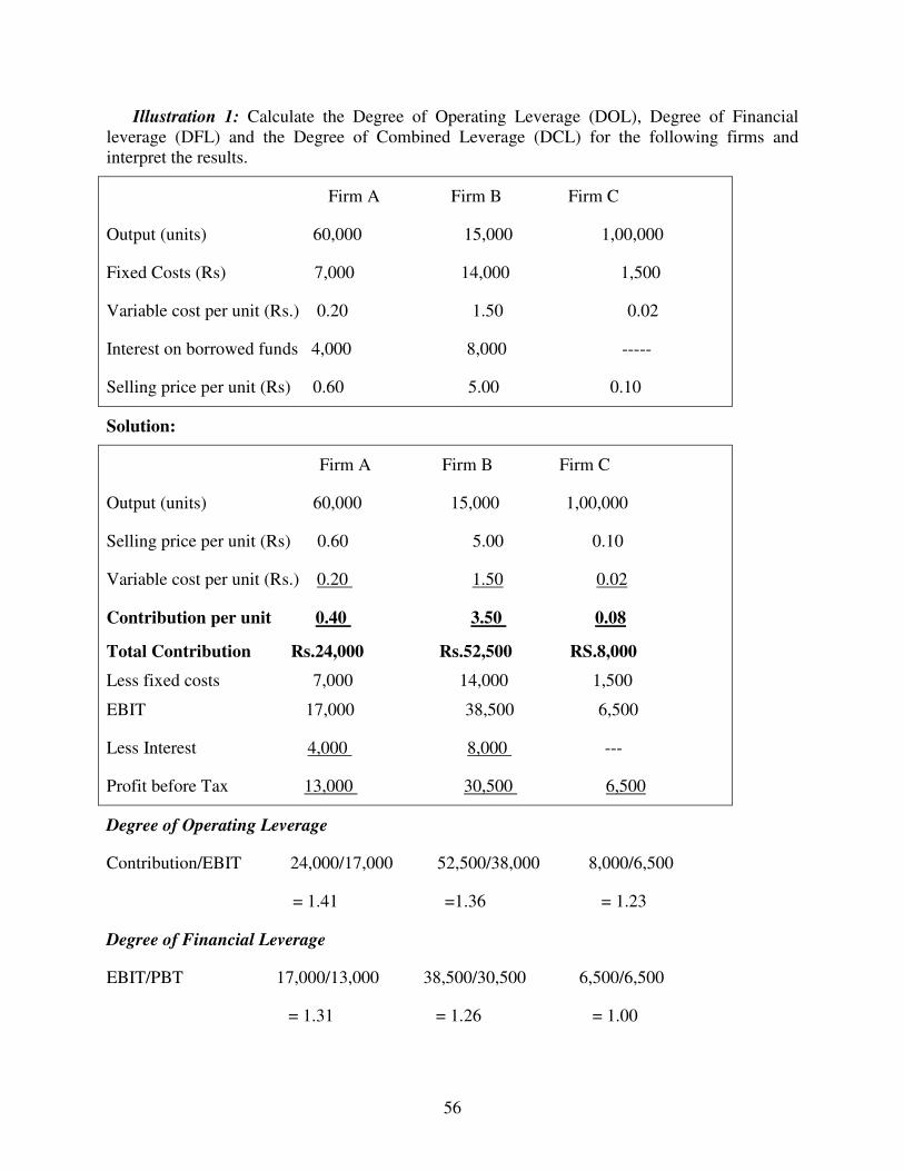
56
Illustration 1: Calculate the Degree of Operating Leverage (DOL), Degree of Financial
leverage (DFL) and the Degree of Combined Leverage (DCL) for the following firms and
interpret the results.
Firm A Firm B Firm C
Output (units) 60,000 15,000 1,00,000
Fixed Costs (Rs) 7,000 14,000 1,500
Variable cost per unit (Rs.) 0.20 1.50 0.02
Interest on borrowed funds 4,000 8,000 -----
Selling price per unit (Rs) 0.60 5.00 0.10
Solution:
Firm A Firm B Firm C
Output (units) 60,000 15,000 1,00,000
Selling price per unit (Rs) 0.60 5.00 0.10
Variable cost per unit (Rs.) 0.20 1.50 0.02
Contribution per unit 0.40 3.50 0.08
Total Contribution Rs.24,000 Rs.52,500 RS.8,000
Less fixed costs 7,000 14,000 1,500
EBIT 17,000 38,500 6,500
Less Interest 4,000 8,000 ---
Profit before Tax 13,000 30,500 6,500
Degree of Operating Leverage
Contribution/EBIT 24,000/17,000 52,500/38,000 8,000/6,500
= 1.41 =1.36 = 1.23
Degree of Financial Leverage
EBIT/PBT 17,000/13,000 38,500/30,500 6,500/6,500
= 1.31 = 1.26 = 1.00

57
Degree of Combined Leverage
Contribution/ EBIT 24,000/13,000 52,500/30,500 8,000/6,500
= 1.85 = 1.72 = 1.23
Illustration 2: A firm has sales of Rs. 10,00,000, variable cost of Rs. 7,00,000 and fixed costs of
Rs. 2,00,000 and debt of Rs. 5,00,000 at 10% rate of interest. What are the operating, financial
and combined leverages. If the firm wants to double its earnings before interest and tax (EBIT),
how much of a rise in sales would be needed on a percentage basis?
Solution:
Statement of Existing Profit
Sales Rs.10,00,000
Less Variable cost 7,00,000
Contribution 3,00,000
Less fixed cost 2,00,000
EBIT 1,00,000
Less Interest @ 10% on 5,00,000 50,000
Profit after Tax 50,000
Operating leverage Contribution/ EBIT = 3,00,000/1,00,000 = 3
Financial Leverage EBIT/PBT = 1,00,000/50,000 = 2
Combined Leverage = 3x 2= 6
Statement of sales needed to double EBIT
Operating Leverage is 3 times i.e. 33 – 1/3% increase in sales volume causes a 100%
increase in operating profit or EBIT. Thus, at the sales of Rs. 13,33,333, operating profit or EBIT
will become Rs. 2,00,000 i.e. double existing one.

58
Verification:
Sales Rs.13,33,333
Variable cost (70%) 9,33,333
Contribution 4,00,000
Fixed Costs 2,00,000
EBIT 2,00,000
Illustration 3: The balance sheet of Well Established Company is as follows:
Liabilities Amount Assets Amount
Equity share capital 60,000 Fixed Assets 1,50,000
Retained Earnings 20,000 Current Assets 50,000
10% long term debt 80,000
Current Liabilities 40,000 ------------
2,00,000 2,00,000
The company’s total assets turnover ratio is 3, its fixed operating costs are Rs.1,00,000
and its variable operating cost ratio is 40%. The income tax rate is 50%. Calculate the different
types of leverages given that the face value of share is Rs.10.
Solution: Total Assets Turnover Ratio = Sales / Total Assets
3 = Sales/2,00,000
Sales 6,00,000
Variable Operating Cost (40%) 2,40,000
Contribution 3,60,000
Less Fixed Operating Cost 1,00,000
EBIT 2,60,000
Less interest (10% of 80,000) 8,000
PBT 2,52,000
Tax at 50% 1,26,000

59
PAT 1,26,000
Number of shares 6,000
EPS Rs.21
Degree of Operating Leverage = Contribution/EBIT
= 3,60,000/2,60,000 = 1.38
Degree of Financial leverage = EBIT / PBT
= 2,60,000/2,52,000 = 1.03
Degree of Combined Leverage =1.38 x 1.03 = 1.42
Illustration 4: The following information is available for ABC & Co.
EBIT Rs. 11,20,000
Profit before Tax 3,20,000
Fixed Costs 7,00,000
Calculate % change in EPS if the sales are expected to increase by 5%.
Solution: In order to find out the % change in EPS as a result of % change in sales, the
combined leverage should be calculated as follows:
Operating Leverage = Contribution/ EBIT
= Rs.11,20,000 + Rs. 7,00,000/11,20,000
= 1.625
Financial Leverage = EBIT / Profit before Tax
= Rs. 11,20,000/3,20,000
= 3.5
Combined Leverage = Contribution/ Profit before Tax = OL x FL
= 1.625 x 3.5 = 5.69
The combined leverage of 5.69 implies that for 1% change in sales level, the % change in
EPS would be 5.69% So, if the sales are expected to increase by 5%, then the % increase in EPS
would be 5 x 5.69 = 28.45%.

60
Illustration 5: The data relating to two companies are as given below:
Company A Company B
Capital Rs.6,00,000 Rs.3,50,000
Debentures Rs. 4,00,000 6,50,000
Output (units) per annum 60,000 15,000
Selling price/unit Rs.30 250
Fixed costs per annum 7,00,000 14,00,000
Variable cost per unit 10 75
You are required to calculate the Operating leverage, Financial leverage and Combined Leverage
of two companies.
Solution: Computation of Operating leverage, Financial Leverage and Combined leverage
Company A Company B
Output (units) per annum 60,000 15,000
Selling price/unit Rs.30 250
Sales Revenue 18,00,000 37,50,000
Less variable costs
@ Rs.10 and Rs.75 6,00,000 11,25,000
Contribution 12,00,000 26,25,000
Less fixed costs 7,00,000 14,00,000
EBIT 5,00,000 12,25,000
Less Interest @ 12%
on debentures 48,000 78,000
PBT 4,52,000 11,47,000
DOL = Contribution/EBIT 12,00,000/5,00,000 26,25,000/12,25,000
= 2.4 = 2.14
DFL = EBIT/ PBT 5,00,000/4,52,000 12,25,000/11,47,000
1.11 =1.07
DCL = DOL x DFL 2.14 x 1.11 = 2.66 2.14 x 1.07 = 2.2
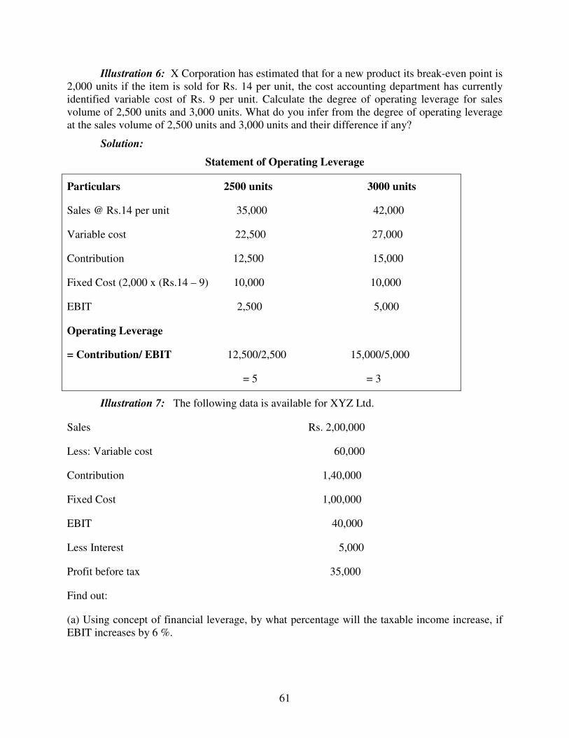
61
Illustration 6: X Corporation has estimated that for a new product its break-even point is
2,000 units if the item is sold for Rs. 14 per unit, the cost accounting department has currently
identified variable cost of Rs. 9 per unit. Calculate the degree of operating leverage for sales
volume of 2,500 units and 3,000 units. What do you infer from the degree of operating leverage
at the sales volume of 2,500 units and 3,000 units and their difference if any?
Solution:
Statement of Operating Leverage
Particulars 2500 units 3000 units
Sales @ Rs.14 per unit 35,000 42,000
Variable cost 22,500 27,000
Contribution 12,500 15,000
Fixed Cost (2,000 x (Rs.14 – 9) 10,000 10,000
EBIT 2,500 5,000
Operating Leverage
= Contribution/ EBIT 12,500/2,500 15,000/5,000
= 5 = 3
Illustration 7: The following data is available for XYZ Ltd.
Sales Rs. 2,00,000
Less: Variable cost 60,000
Contribution 1,40,000
Fixed Cost 1,00,000
EBIT 40,000
Less Interest 5,000
Profit before tax 35,000
Find out:
(a) Using concept of financial leverage, by what percentage will the taxable income increase, if
EBIT increases by 6 %.

62
(b) Using the concept of operating leverage, by what percentage will EBIT increase if there is
10% increase in sales and,
(c) Using the concept of leverage, by what percentage will the taxable income increase if the
sales increase by 6%. Also verify the results in view of the above figures.
Solution:
(i) Degree of Financial Leverage:
FL = EBIT/Profit before Tax = 40,000/35,000 = 1.15
If EBIT increases by 6%, the taxable income will increase by 1.15 x 6 = 6.9% and it may be
verified as follows:
EBIT (after 6% increase) Rs. 42,400
Less Interest 5,000
Profit before Tax 37,400
Increase in taxable income is Rs. 2,400 i.e 6.9% of Rs. 35,000
(ii) Degree of Operating Leverage:
OL = Contribution / EBIT = 1,40,000/40,000 = 3.50
If sale increases by 10%, the EBIT will increase by 3.50 x 10 = 35% and it may be verified as
follows:
Sales (after 10% increase) Rs. 2,20,000
Less variable expenses @ 30% 66,000
Contribution 1,54,000
Less Fixed cost 1,00,000
EBIT 54,000
Increase in EBIT is Rs. 14,000 i.e 35% of Rs. 40,000
(iii) Degree of Combined leverage
CL = Contribution/ Profit before tax = 1,40,000/35,000 = 4
If sales increases by 6%, the profit before tax will increase by 4x6= 24% and it maybe verified as
follows:

63
Sales (after 6% increase) Rs. 2,12,000
Less Variable expenses@ 30% 63,600
Contribution 1,48,400
Less Fixed cost 1,00,000
EBIT 48,400
Less Interest 5,000
Profit before tax 43,400
Increase in Profit before tax is Rs. 8,400 i.e 24% of Rs. 35,000
Lets Sum Up
� In Leverage analysis the relationship between two interrelated variables is established. In
financial management Operating leverage, financial leverage and Combined Leverage is
calculated.
� The Operating relationship establishes the relationship between sales and EBIT. It
measures the effect of change in sales revenue on the level of EBIT.
� Operating leverage appears as a result of fixed cost.
� The financial leverage measures the responsiveness of the EPS for given change in EBIT.
� The financial leverage appears as a result of fixed financial charge i.e. interest and
preference dividend.
� Combined leverage may also be ascertained to measures the % change in EPS for a %
change in the sales.
QUESTIONS
1 Distinguish between operating leverage and financial leverage. How the two leverages
can be measured?
2 Explain the concept of financial leverage. Examine the impact of financial leverage on
the EPS. Does the financial Leverage always increases the EPS?

64
UNIT 4
1
DIVIDEND DECISION AND VALUATION OF THE FIRM
Smriti Chawla Shri Ram College of Commerce
University of Delhi
Introduction
The term dividend refers to that profits of a company which is distributed by company
among its shareholders. It is the reward of the shareholders for investments made by them in the
shares of the company. A company may have preference share capital as well as equity share
capital and dividends may be paid on both types of capital. The investors are interested in
earning the maximum return on their investments and to maximize their wealth on the other
hand, a company needs to provide funds to finance its long-term growth. If a company pays out
as dividend most of what it earns, then for Business requirements and further expansion it will
have to depend upon outside resources such as issue of debt or a new shares. Dividend policy of
a firm, thus affects both long-term financing and wealth of shareholders.
Concept and Significance
The dividend decision is one of the three basic decisions which a financial manager may
be required to take, the other two being the investment decisions and the financing decisions. In
each period any earning that remains after satisfying obligations to the creditors, the government
and the preference shareholders can either be retained or paid out as dividends or bifurcated
CHAPTER OBJECTIVES
� Introduction � Concept and Significance � Dividend Decision and Valuation of Firms
� Relevance Concept of Dividend
Walter’s Approach Gordon’s Approach
� Irrelevance Concept of Dividend
Residual Approach Modigliani & Miller Approach
� Lets Sum Up � Questions
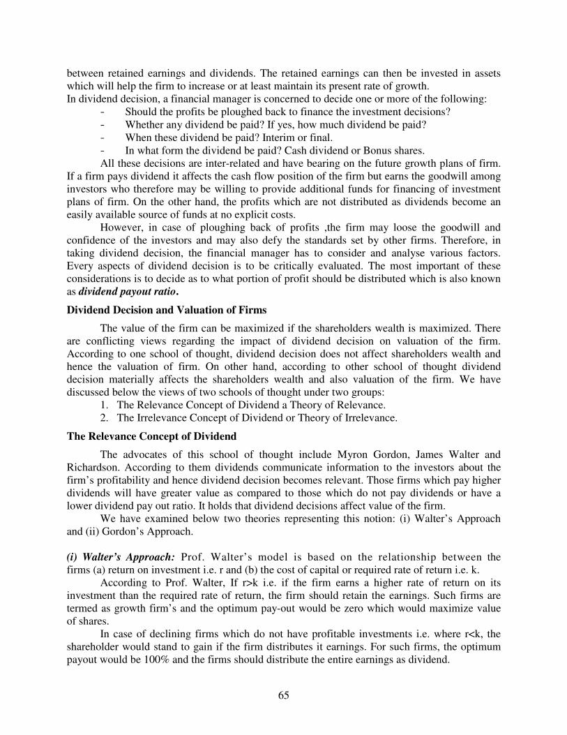
65
between retained earnings and dividends. The retained earnings can then be invested in assets
which will help the firm to increase or at least maintain its present rate of growth.
In dividend decision, a financial manager is concerned to decide one or more of the following:
- Should the profits be ploughed back to finance the investment decisions?
- Whether any dividend be paid? If yes, how much dividend be paid?
- When these dividend be paid? Interim or final.
- In what form the dividend be paid? Cash dividend or Bonus shares.
All these decisions are inter-related and have bearing on the future growth plans of firm.
If a firm pays dividend it affects the cash flow position of the firm but earns the goodwill among
investors who therefore may be willing to provide additional funds for financing of investment
plans of firm. On the other hand, the profits which are not distributed as dividends become an
easily available source of funds at no explicit costs.
However, in case of ploughing back of profits ,the firm may loose the goodwill and
confidence of the investors and may also defy the standards set by other firms. Therefore, in
taking dividend decision, the financial manager has to consider and analyse various factors.
Every aspects of dividend decision is to be critically evaluated. The most important of these
considerations is to decide as to what portion of profit should be distributed which is also known
as dividend payout ratio.
Dividend Decision and Valuation of Firms
The value of the firm can be maximized if the shareholders wealth is maximized. There
are conflicting views regarding the impact of dividend decision on valuation of the firm.
According to one school of thought, dividend decision does not affect shareholders wealth and
hence the valuation of firm. On other hand, according to other school of thought dividend
decision materially affects the shareholders wealth and also valuation of the firm. We have
discussed below the views of two schools of thought under two groups:
1. The Relevance Concept of Dividend a Theory of Relevance.
2. The Irrelevance Concept of Dividend or Theory of Irrelevance.
The Relevance Concept of Dividend
The advocates of this school of thought include Myron Gordon, James Walter and
Richardson. According to them dividends communicate information to the investors about the
firm’s profitability and hence dividend decision becomes relevant. Those firms which pay higher
dividends will have greater value as compared to those which do not pay dividends or have a
lower dividend pay out ratio. It holds that dividend decisions affect value of the firm.
We have examined below two theories representing this notion: (i) Walter’s Approach
and (ii) Gordon’s Approach.
(i) Walter’s Approach: Prof. Walter’s model is based on the relationship between the
firms (a) return on investment i.e. r and (b) the cost of capital or required rate of return i.e. k.
According to Prof. Walter, If r>k i.e. if the firm earns a higher rate of return on its
investment than the required rate of return, the firm should retain the earnings. Such firms are
termed as growth firm’s and the optimum pay-out would be zero which would maximize value
of shares.
In case of declining firms which do not have profitable investments i.e. where r<k, the
shareholder would stand to gain if the firm distributes it earnings. For such firms, the optimum
payout would be 100% and the firms should distribute the entire earnings as dividend.
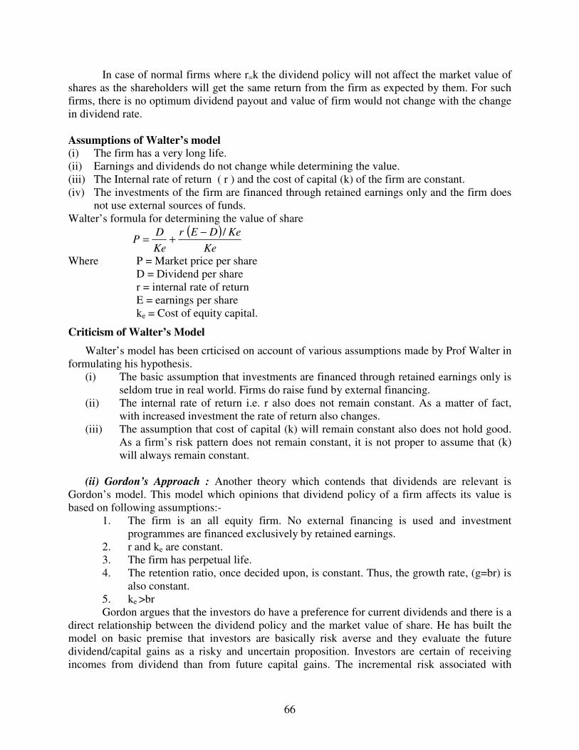
66
In case of normal firms where r=k the dividend policy will not affect the market value of
shares as the shareholders will get the same return from the firm as expected by them. For such
firms, there is no optimum dividend payout and value of firm would not change with the change
in dividend rate.
Assumptions of Walter’s model
(i) The firm has a very long life.
(ii) Earnings and dividends do not change while determining the value.
(iii) The Internal rate of return ( r ) and the cost of capital (k) of the firm are constant.
(iv) The investments of the firm are financed through retained earnings only and the firm does
not use external sources of funds.
Walter’s formula for determining the value of share
( )
Ke
KeDEr
Ke
DP
/−+=
Where P = Market price per share
D = Dividend per share
r = internal rate of return
E = earnings per share
ke = Cost of equity capital.
Criticism of Walter’s Model
Walter’s model has been crticised on account of various assumptions made by Prof Walter in
formulating his hypothesis.
(i) The basic assumption that investments are financed through retained earnings only is
seldom true in real world. Firms do raise fund by external financing.
(ii) The internal rate of return i.e. r also does not remain constant. As a matter of fact,
with increased investment the rate of return also changes.
(iii) The assumption that cost of capital (k) will remain constant also does not hold good.
As a firm’s risk pattern does not remain constant, it is not proper to assume that (k)
will always remain constant.
(ii) Gordon’s Approach : Another theory which contends that dividends are relevant is
Gordon’s model. This model which opinions that dividend policy of a firm affects its value is
based on following assumptions:-
1. The firm is an all equity firm. No external financing is used and investment
programmes are financed exclusively by retained earnings.
2. r and ke are constant.
3. The firm has perpetual life.
4. The retention ratio, once decided upon, is constant. Thus, the growth rate, (g=br) is
also constant.
5. ke >br
Gordon argues that the investors do have a preference for current dividends and there is a
direct relationship between the dividend policy and the market value of share. He has built the
model on basic premise that investors are basically risk averse and they evaluate the future
dividend/capital gains as a risky and uncertain proposition. Investors are certain of receiving
incomes from dividend than from future capital gains. The incremental risk associated with

67
capital gains implies a higher required rate of return for discounting the capital gains than for
discounting the current dividends. In other words, an investor values current dividends more
highly than an expected future capital gain.
Hence, the “bird-in-hand” argument of this model suggests that dividend policy is relevant,
as investors prefer current dividends as against the future uncertain capital gains. When investors
are certain about their returns they discount the firm’s earnings at lower rate and therefore
placing a higher value for share and that of firm. So, the investors require a higher rate of return
as retention rate increases and this would adversely affect share price.
Symbolically: -
( )
brKe
bEP
−
−=
1
where P = Market price of equity share
E = Earnings per share of firm.
b = Retention Ratio (1 – payout ratio)
r = Rate of Return on Investment of the firm.
Ke = Cost of equity share capital.
br = g i.e. growth rate of firm.
The Irrelevance Concept of Dividend
The other school of thought on dividend policy and valuation of the firm argues that what
a firm pays as dividends to share holders is irrelevant and the shareholders are indifferent about
receiving current dividend in future. The advocates of this school of thought argue that dividend
policy has no effect on market price of share. Two theories have been discussed here to focus on
irrelevance of dividend policy for valuation of the firm which are as follows:
1. Residual’s Theory of Dividend
According to this theory, dividend decision has no effect on the wealth of shareholders or
the prices of the shares and hence it is irrelevant so far as valuation of firm is concerned. This
theory regards dividend decision merely as a part of financing decision because earnings
available may be retained in the business for re-investment. But if the funds are not required in
the business they may be distributed as dividends. Thus, the decision to pay dividend or retain
the earnings may be taken as residual decision. This theory assumes that investors do not
differentiate between dividends and retentions by firm. Their basic desire is to earn higher return
on their investment. In case the firm has profitable opportunities giving higher rate of return than
cost of retained earnings, the investors would be content with the firm retaining the earnings to
finance the same. However, if the firm is not in a position to find profitable investment
opportunities, the investors would prefer to receive the earnings in the form of dividends. Thus, a
firm should retain earnings if it has profitable investment opportunities otherwise it should pay
them as dividends.
Under the Residuals theory, the firm would treat the dividend decision in three steps:
o Determining the level of capital expenditures which is determined by the investment
opportunities.
o Using the optimal financing mix, find out the amount of equity financing need to support
the capital expenditure in step (i) above
o As the cost of retained earnings kr is less than the cost of new equity capital, the retained
earnings would be used to meet the equity portions financing in step (ii) above. If
68
available profits are more than this need, then the surplus may be distributed as dividends
of shareholder. As far as the required equity financing is in excess of the amount of
profits available, no dividends would be paid to the shareholders.
Hence, in residual theory the dividend policy is influenced by (i) the company’s
investment opportunities and (ii) the availability of internally generated funds, where dividends
are paid only after all acceptable investment proposals have been financed. The dividend policy
is totally passive in nature and has no direct influence on the market price of the share.
2. Modigliani and Miller Approach (MM Model)
Modigliani and Miller have expressed in the most comprehensive manner in support of
theory of irrelevance. They maintain that dividend policy has no effect on market prices of shares
and the value of firm is determined by earning capacity of the firm or its investment policy. As
observed by M.M, “Under conditions of perfect capital markets, rational investors, absence of
tax discrimination between dividend income and capital appreciation, given the firm’s
investment policy, its dividend policy may have no influence on the market price of shares”.
Even, the splitting of earnings between retentions and dividends does not affect value of firm.
Assumptions of MM Hypothesis
(1) There are perfect capital markets.
(2) Investors behave rationally.
(3) Information about company is available to all without any cost.
(4) There are no floatation and transaction costs.
(5) The firm has a rigid investment policy.
(6) No investor is large enough to effect the market price of shares.
(7) There are either no taxes or there are no differences in tax rates applicable to
dividends and capital gains.
The Argument of MM
The argument given by MM in support of their hypothesis is that whatever increase in
value of the firm results from payment of dividend, will be exactly off set by achieve in market
price of shares because of external financing and there will be no change in total wealth of the
shareholders. For example, if a company, having investment opportunities distributes all its
earnings among the shareholders, it will have to raise additional funds from external sources.
This will result in increase in number of shares or payment of interest charges, resulting in fall in
earnings per share in future. Thus whatever a shareholder gains on account of dividend payment
is neutralized completely by the fall in the market price of shares due to decline in expected
future earnings per share. To be more specific, the market price of share in beginning of period is
equal to present value of dividends paid at end of period plus the market price of shares at end of
period plus the market price of shares at end of the period. This can be put in form of following
formula:-
P0 = D1 + P1
1 + Ke
where
PO = Market price per share at beginning of period.
D1 = Dividend to be received at end of period.
P1 = Market price per share at end of period.
Ke = Cost of equity capital.

69
The value of P1 can be derived by above equation as under.
( ) 11 1 DKePPO
−+=
The MM Hypothesis can be explained in another form also presuming that investment
required by the firm on account of payment of dividends is financed out of the new issue of
equity shares.
In such a case, the number of shares to be issued can be computed with the help of the
following equation:
( )
1
11
P
nDEm
−=
Further, the value of the firm can be ascertained with the help of the following formula:
( ) ( )
Ke
EIPmnnP
O
+
−−+=
1
1
where,
m = number of shares to be issued.
I = Investment required.
E = Total earnings of the firm during the period.
P1 = Market price per share at the end of the period.
Ke = Cost of equity capital.
n = number of shares outstanding at the beginning of the period.
D1 = Dividend to be paid at the end of the period.
nPO = Value of the firm.
This equation shows that dividends have no effect on the value of the firm when external
financing is used. Given the firm’s investment decision, the firm has two alternatives, it can
retain its earnings to finance the investments or it can distribute the earnings to the shareholders
as dividends and can arise an equal amount externally. If the second alternative is preferred, it
would involve arbitrage process. Arbitrage refers to entering simultaneously into two
transactions which exactly balance or completely offset each other. Payment of dividends is
associated with raising funds through other means of financing. The effect of dividend payment
on shareholder’s wealth will be exactly offset by the effect of raising additional share capital.
When dividends are paid to the shareholder, the market price of the shares will increase. But the
issue of additional block of shares will cause a decline in the terminal value of shares. The
market price before and after the payment of the dividend would be identical. This theory thus
signifies that investors are indifferent about dividends and capital gains. Their principal aim is to
earn higher on investment. If a firm has investment opportunities at hand promising higher rate
of return than cost of capital, investor will be inclined more towards retention. However, if the
expected return is likely to be less than what it would cost, they would be least interested in
reinvestment of income. Modigiliani and Miller are of the opinion that value of a firm is
determined by earning potentiality and investment policy and never by dividend decision.
Criticism of MM Approach
MM Hypothesis has been criticized on account of various unrealistic assumptions as
given below.
1. Perfect capital markets does not exist in reality.
2. Information about company is not available to all persons.
70
3. The firms have to incur floatation costs which issuing securities.
4. Taxes do exit and there is normally different tax treatment for dividends and capital
gains.
5. The firms do not follow rigid investment policy.
6. The investors have to pay brokerage, fees etc. which doing any transaction.
7. Shareholders may prefer current income as compared to further gains.
Lets Sum Up
• Dividend decision is an important decision, which a financial manager has to take. It
refers to that profits of a company which is distributed by company among its
shareholders.
• There has been a difference of opinion on the effect of dividend policy on value of
firm. Two schools of thought have emerged on relationship between dividend policy
and value of firm.
• On one hand Walter model and Gordon model consider dividend as relevant for value
of firm as investors prefer current dividend over future dividend.
• On other hand Residuals Approach and MM Model consider dividend is irrelevant for
value of firm. The detention of profit for re-investment is important. MM Model have
introduced arbitrage process to prove that value of firm remain same whether firm
pays dividend or not.
• Different models market price can be ascertained as :
Walter’s Model = ( )
Ke
KeDEr
Ke
DP
/−+=
Gordon Model = ( )
beKe
bEP
−
−=
1
MM Model = Ke
PDP
O
+
+=
1
11
QUESTIONS
1 Explain the Modigliani-Miller hypothesis of dividend irrelevance. Does this dividend
irrelevance. Does this hypothesis suffer from deficiencies?
2 How far do you agree that dividends are irrelevant?
3 In Walter’s Approach, the dividend policy of firm depends on availability of investment
opportunity and relationship between firm’s internal rate of return and its cost of capital.
Discuss what are shortcomings of this view?
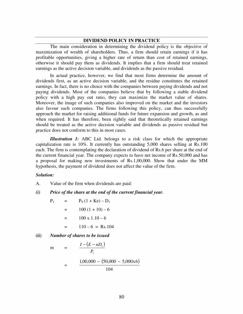
80
DIVIDEND POLICY IN PRACTICE
The main consideration in determining the dividend policy is the objective of
maximization of wealth of shareholders. Thus, a firm should retain earnings if it has
profitable opportunities, giving a higher rate of return than cost of retained earnings,
otherwise it should pay them as dividends. It implies that a firm should treat retained
earnings as the active decision variable, and dividends as the passive residual.
In actual practice, however, we find that most firms determine the amount of
dividends first, as an active decision variable, and the residue constitutes the retained
earnings. In fact, there is no choice with the companies between paying dividends and not
paying dividends. Most of the companies believe that by following a stable dividend
policy with a high pay out ratio, they can maximize the market value of shares.
Moreover, the image of such companies also improved on the market and the investors
also favour such companies. The firms following this policy, can thus successfully
approach the market for raising additional funds for future expansion and growth, as and
when required. It has therefore, been rightly said that theoretically retained earnings
should be treated as the active decision variable and dividends as passive residual but
practice does not conform to this in most cases.
Illustration 1: ABC Ltd. belongs to a risk class for which the appropriate
capitalization rate is 10%. It currently has outstanding 5,000 shares selling at Rs.100
each. The firm is contemplating the declaration of dividend of Rs.6 per share at the end of
the current financial year. The company expects to have net income of Rs.50,000 and has
a proposal for making new investments of Rs.1,00,000. Show that under the MM
hypothesis, the payment of dividend does not affect the value of the firm.
Solution:
A. Value of the firm when dividends are paid:
(i) Price of the share at the end of the current financial year.
P1 = P0 (1 + Ke) – D1
= 100 (1 + 10) – 6
= 100 x 1.10 – 6
= 110 – 6 = Rs.104
(ii) Number of shares to be issued
m = ( )
1
1
P
nDEI −−
= ( )
104
6x000,5000,50000,00,1 −−

81
= 104
000,80
(iii) Value of the firm
nP0 = ( ) ( )
Ke1
E1Pmn 1
+
−−+
=
( )
101
000,50000,00,1104104
000,80000,5
+
−−×
−
=
( )
10.1
000,501
104
104
000,80000,20,5−×
+
= 10.1
000,50000,00,6 −
= 10.1
000,50,5
= Rs.5,00,000
B. Value of the firm when dividends are not paid:
(i) Price per share at the end of the current financial year
P1 = P0 (1 + ke) – D1
= 100 (1+.10)-0
= 100×1.10
= Rs. 110
(ii) Number of shares to be issued
m = ( )
1
1
P
nDEI −−
= 110
)0000,50(000,00,1 −−
= 110
000,50
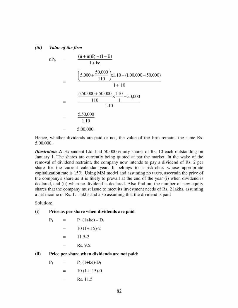
82
(iii) Value of the firm
nP0 = ke1
)EI(P)mn( 1
+
−−+
= 10.1
)000,50000,00,1(10.1x110
000,50000,5
+
−−
+
= 10.1
000,501
110
110
000,50000,50,5−×
+
= 10.1
000,50,5
= 5,00,000.
Hence, whether dividends are paid or not, the value of the firm remains the same Rs.
5,00,000.
Illustration 2: Expandent Ltd. had 50,000 equity shares of Rs. 10 each outstanding on
January 1. The shares are currently being quoted at par the market. In the wake of the
removal of dividend restraint, the company now intends to pay a dividend of Rs. 2 per
share for the current calendar year. It belongs to a risk-class whose appropriate
capitalization rate is 15%. Using MM model and assuming no taxes, ascertain the price of
the company's share as it is likely to prevail at the end of the year (i) when dividend is
declared, and (ii) when no dividend is declared. Also find out the number of new equity
shares that the company must issue to meet its investment needs of Rs. 2 lakhs, assuming
a net income of Rs. 1.1 lakhs and also assuming that the dividend is paid
Solution:
(i) Price as per share when dividends are paid
P1 = P0 (1+ke) – D1
= 10 (1+.15)-2
= 11.5-2
= Rs. 9.5.
(ii) Price per share when dividends are not paid:
P1 = P0 (1+ke)-D1
= 10 (1+. 15)-0
= Rs. 11.5

83
(iii) Number of new equity shares to be issued if dividend is paid
m = 1
1
P
)nDE(I −−
= 5.9
)2000,50000,10,1(000,00,2 ×−−
= 5.9
000,90,1
= 20,000 shares
Illustration 3: The following information is available in respect of a firm:
Capitalisation rate = 10%
Earnings per share = Rs. 50
Assumed rate of return on investments:
(i) 12%
(ii) 8%
(iii) 10%
Show the effect of dividend policy on market price of shares applying Walter's formula
when dividend pay out ratio is (a) 0% (b) 20%, (c) 40%, (d) 80%, and (e) 100%
Solution :
P = e
e
e k
k/)DE(r
k
D −+
Effect of dividend Policy on market price of shares
(i) r = 12% (ii) r = 8% (iii) r = 100
(a) When dividend pay-out ratio is 0%
P = 10.
10./)050(12.
10.
0 −+ P =
10.
10./)050(8.
10.
0 −+ P =
10.
10./)050(10.
10.
0 −+
= 10.
)50(10.
12.
0+ = 10.
)50(10.
8.
0+ = 10.
)50(10.
10.
0+
= Rs. 600 = Rs. 400 = Rs. 500

84
(b) When dividend pay-out is 20%
P = )1050(10.
10
12.
10.
10−+ P =
10.
)1050(10.
8.
10.
10−
+ P = 10.
)1050(10.
10.
10.
10−
+
= 10
48100+
= 100+320 = 100+400
= Rs. 580 = Rs. 420 = Rs. 500
(c) When dividend pay out is 40%
P = )2050(10.
10.
12.
10.
20−+ P =
10.
)2050(10.
8.
10.
20−
+ P = 10.
)2050(10.
10.
10.
20−
+
= 200 + 10.
36
= 200+240 = 200+300
= Rs. 560 = Rs. 440 = Rs. 500
(d) When dividend pay-out is 80%
P = )4050(10.
10.
12.
10.
40−+ P =
10.
)4050(10.
8.
10.
40−
+ P = 10.
)4050(10.
10.
10.
40−
+
= 400+120 = 400+80 = 400+100
= Rs. 520 = Rs. 480 = Rs. 500
(e) When dividend pay-out is 100%
P = 10.
)5050(10.
12.
10.
50−
+ P = 10.
)5050(10.
8.
10.
50−
+ P = 10.
)5050(10.
10.
10.
50−
+
= 500+0 = 500+0 = 500+0
= Rs. 500 = Rs. 500 = Rs. 500
Conclusion: From the above analysis we can draw the conclusion that when,
(i) r >k, the company should retain the profits, i.e., when r=12%. ke=10%;
(ii) r is 8%, i.e., r<k, the pay-out should be high; and
(iii) r is 10%; i.e., r=k; the dividend pay-out does not affect the price of the
share.

85
Illustration 4: The earnings per share of company are Rs. 8 and the rate of
capitalisation applicable to the company is 10%. The company has before it an option of
adopting a payout ratio of 25% or 50% or 75%. Using Walter's formula of dividend
payout, compute the market value of the company's share if the productivity of retained
earnings is (i) 15% (ii) 10% and (iii) 5%
Solution:
According to Walter's formula
P = ke
ke/)DE(r
ke
D −+
where, P = Market price per share
D = Dividend per share
R = Internal rate of return of productivity of retained earnings.
E = Earnings per share, and
ke = Cost of equity capital or capitalisation rate.
Computation of Market Value of Company’s Shares
(i) r=15% (ii) r=10% (iii) r=5%
(a) When dividend payout ratio is 25%
P = 10.
10./)28(15.
10.
2 −+ P =
10.
10./)28(10.
10.
2 −+ P =
10.
10./)28(5.
10.
2 −+
= 10.
)6(10.
15.
10.
2+ =
10.
)6(10.
10.
10.
2+ =
10.
)6(10.
5.
10.
2+
= 10.
9
10.
2+ =
10.
6
10.
2+ =
10.
3
10.
2+
= 10.
11 =
10.
8 =
10.
5
= Rs. 110 = Rs. 80 = Rs. 50
(b) When dividend payout ratio is 50%
P = 10.
10./)48(15.
10.
4 −+ P =
10.
10./)48(10.
10.
4 −+ P =
10.
10./)48(5.
10.
4 −+
= 10.
)4(10.
15.
10.
4+ =
10.
)4(10.
10.
10.
4+ =
10.
)4(10.
5.
10.
4+

86
= 10.
6
10.
4+ =
10.
4
10.
4+ =
10.
2
10.
4+
= 10.
10 =
10.
8 =
10.
6
= Rs. 100 = Rs. 80 = Rs. 60
(c) When dividend payout ratio is 75%
P = 10.
10./)68(15.
10.
6 −+ P =
10.
10./)68(10.
10.
6 −+ P =
10.
10./)68(5.
10.
6 −+
= 10.
)2(10.
15.
10.
6+ =
10.
)2(10.
10.
10.
6+ =
10.
)2(10.
5.
10.
6+
= 10.
3
10.
6+ =
10.
2
10.
6+ =
10.
1
10.
6+
= 10.
9 =
10.
8 =
10.
7
= Rs. 90 = Rs. 80 = Rs. 70
Illustration 5: The earnings per share of a share of the face value of Rs.100 to
PQR Ltd. is Rs.20. It has a rate of return of 25%. Capitalisation rate of its risk class is
12.5%. If Walter's model is used:
a) What should be the optimum payout ratio?
b) What should be the market price per share if the payout ratio is zero?
c) Suppose, the company has a payout of 25% of EPS, what would be the price per
share?
Solution: As per Walter's formula, the price of the share is
e
e
e k
DEkr
k
DP
)()/( −+=
a) If r > ke, the value of share will increase with every increase in retention. The
price of the share should be the maximum when the firm retains all the earnings.
Thus, the optimum payout ratio is zero for PQR Ltd.
b) Calculation of market price when the payout ratio is zero.

87
320.125.0
)20()125.0/25(.0RsP =
+=
c) Payout of 25% of EPS i.e., 25% of Rs.20 = Rs.5 per share:
k
DEkr
k
DP
e
e
)()/( −+=
280.125.0
)520()125.0/25(.5Rs=
−+=
Illustration 6: Determine the market value of equity shares of the company
from the following information:
Earnings of the company Rs.5,00,000
Dividend paid 3,00,000
Number of shares outstanding 1,00,000
Price-earning ratio 8
Rate of return on investment 15%
Are you satisfied with the current dividend policy of the firm? If not, what should
be the optimal dividend payout ratio? Use Walter's Model.
Solution:
EPS
priceMarketRatioEarningsPrice =
58
priceMarket=
So, Market price = 8 x 5 = Rs.40
5.000,00,1
000,00,5RsEPS ==
3.000,00,1
000,00,3RsDPS ==
Dividend payout ratio = %601005
3100 == xx
EPS
DPS
Walter's Model: As the P/E ratio is given 8, and the ke may be taken as 1/8 = .125
Since, this is a growth firm having rate of return (15%) > cost of capital of 12.5%, the
company will maximize its market price if it retains 100% of profits. The current market
price of Rs..40 (based on P/E Ratio can be increased by reducing the payout ratio. If the
company opts for 100% retention (i.e. 0% payout), the market price of the share as per
Walter's formula would be as follows:
e
e
e k
DEkr
k
DP
)()/( −+=

88
48.125.
)5()125./15(.
125.
0RsP =+=
So, the firm can increase the market price of the share up to Rs.48 by increasing the
retention ratio to 100% or in other words, the optimal dividend payout for the firm is 0.
Illustration 7: The earnings per share (EPS) of a company is Rs.10. It has an
internal rate of return of 15% and the capitalization rate of its risk class is 12.5%. If
Walter's Model is used –
(i) What should be the optimum payout ratio of the company?
(ii) What would be the price of the share at this payout?
(iii) How shall the price of the share be affected, if a different payout were employed?
Solution: Walter's model to determine share value:
ee k
DEk
r
k
DPshareperpriceMarket
)(1
0
−
+==
where, D = Dividend per share, E = Earning per share, r = return on Investment and ke =
Capitalisation rate
If r > ke, the value of the share will increase as retention increases. The price of
the share would be maximum when the firm retains all the earnings. Thus, the optimum
payout ratio in this case is zero. When the optimum payment is zero, the price of the
share is:
96.125.0
12
125.0
)010()125.0/15.0(0RsP ==
−+=
If the firm chooses a payout other than zero, the price of the share will fall.
Suppose, the firm has a payment of 20%, the price of the share will be:
80.92.125.0
60.11
125.0
)210()125.0/15.0(2RsP ==
−+=
Illustration 8 : From the following information supplied to you, ascertain whether
the firm is following an optimal dividend policy as per Walter's model?
Total Earnings Rs.2,00,000
Number of equity shares (of Rs.100 each) 20,000
Dividend paid 1,50,000
Price/Earning ratio 12.5
The firm is expected to maintain its rate of return on fresh investment. Also find
out what should be the P/E ratio at which the dividend policy will have no effect on the
value of the share?
Solution: The EPS of the firm is Rs.10 (i.e., Rs.2,00,000/20,000). The P/E Ratio
is given at 12.5 and the cost of capital, ke may be taken at the inverse of P/E ratio.
Therefore, ke is 8 (i.e., 1/12.5). The firm is distributing total dividends of Rs.1,50,000

89
among 20,000 shares giving a dividend per share of Rs.7.50. The value of the share as
per Walter's model may be found as follows:
e
e
e k
DEkr
k
DP
)()/( −+=
.81.132.08.
)5.710()08./10(.
08.
50.7Rs=
−+=
The firm has a dividend payout of 75% (i.e., Rs.1,50,000) out of total earnings of
Rs.2,00,000. Since, the rate of return of the firm, r, is 10% and it is more than the ke of
8%, therefore, by distributing 75% of earnings, the firm is not following an optimal
dividend policy.
In this case, the optimal dividend policy for the firm would be to pay zero
dividend and in such a situation, the market price would be
e
e
e k
DEkr
k
DP
)()/( −+=
25.156.08.
)5.710()08./10(.
08.
50.7Rs=
−+=
So, the market price of the share can be increased by following a zero payout.
The P/E ratio at which the dividend policy will have no effect on the value of the
firm is such at which the ke would be equal to the rate of return, r, of the firm. The ke
would be 10% (= r) at the P/E ratio of 10. Therefore, at the P/E ratio of 10, the dividend
policy would have no effect on the value of the firm.
Illustration 9: A company has total investment of Rs.5,00,000 assets and 50,000
outstanding equity shares of Rs.10 each. It earns a rate of 15% on its investments, and
has a policy of retaining 50% of the earnings. If the appropriate discount rate for the firm
is 10%, determine the price of its share using Gordon Model. What shall happen to the
price, if the company has a payout of 80% or 20%.
Solution: The Gordon' share valuation model is as under:
brk
bEPSP
−
−=
)1()(0
where, b = Retention ratio = .50 or .20 or .80
k = discount rate = .10
r = rate of return = .15
EPS = .15x10 = Rs.1.50
At a payment of 50%, the price of the share is:

90
30.025.0
75.0
5.015.010.0
1015.0)5.01(0 Rs
x
xP ==
−
−=
At a payment of 80%, the price of the share is:
14.17.007.0
20.1
2.015.010.0
1015.0)2.01(0 Rs
x
xP ==
−
−=
When the payment is 20%, the price of the share is:
15.02.0
30.0
8.015.010.0
1015.0)8.01(0 Rs
x
xP =
−=
−
−=
In the last case, the share price is negative which is unrealistic.
Illustration 10: Assuming that rate of return expected by investor is 11%; internal
rate of return is 12%; and earnings per share is Rs.15, calculate price per share by
'Gordon Approach' method if dividend payout ratio is 10% and 30%.
Solution : As per Gordon’s Approach, re bk
bEP
−
−=
)1(0
In the given case, ke = 11%
r = 12%
EPS = Rs.15
If Dividend Payout is 10%, then retention ratio, b, is 90%.
750.002.
15
9.12.11
)9.1(150 Rs
xP ==
−
−=
If Dividend Payout is 30%, then retention ratio, b is 70%.
08.173.026.
5.4
7.12.11.
)7.1(150 Rs
xP ==
−=
Illustration 11: Textrol Ltd. has 80,000 shares outstanding. The current market
price of these shares is Rs.15 each. The company expect a net profit of Rs.2,40,000
during the year and it belongs to a risk-class for which the appropriate capitalisation rate
has been estimated to be 20%. The Company is considering dividend of Rs.2 per share
for the current year.
a) What will be the price of the share at the end of the year (i) if the dividend is paid
and (ii) if the dividend is not paid?
(b) How many new shares must the Co. issue if the dividend is paid and the Co. needs
Rs.5,60,000 for an approved investment expenditure during the year? Use MM
model for the calculation.
Solution:
As per MM model, the current market price of the share, P0, is
)(1
1110 PD
kP
e
++
=
So, if the firm pays a dividend of Rs.2, the price at the end of year 1, P1, is
)2(201
115 1P+
+=

91
)2(20.1
115 1P+=
P1 = Rs.16
If the dividend is not paid, the price would be
)(1
1110 PD
kP
e
++
=
)0(20.1
115 1P+
+= = P1 = Rs.18
No. of new share, m, to be issued if the company pays a dividend of Rs.2:
mP1 = 1-(E-nD1)
m x16 = 5,60,000-[2,40,000-(80,000x2)]
m x16 = 5,60,000-80,000
m = 4,80,000/16=30,000 new shares.
So, the company should issue 30,000 new shares at the rate of Rs.16 per share in
order to finance its investment proposals.

92
UNIT 5
1
WORKING CAPITAL: MANAGEMENT AND FINANCE
Smriti Chawla Shri Ram College of Commerce
University of Delhi Delhi
Meaning of Working Capital
Capital required for a business can be classified under two main categories viz.
(i) Fixed capital
(ii) Working capital.
Every business needs funds for two purposes for its establishment and to carry out its day-to-
day operations. Long-term funds are required to create production facilities through purchase of
fixed assets such as plant and machinery, land, Building etc. Investments in these assets
represent that part of firm’s capital which is blocked on permanent basis and is called fixed
capital. Funds are also needed for short-term purposes for purchase of raw materials, payment of
wages and other day-to-day expenses etc. These funds are known as working capital which is
also known as Revolving or circulating capital or short term capital. According to Shubin,
“Working capital is amount of funds necessary to cover the cost of operating the enterprise”.
CHAPTER OBJECTIVES
� Meaning and Concept of Working Capital � Classification or Kinds of Working Capital � Importance or Advantages of Adequate Working Capital � Excess or Inadequate Working Capital � Need or Objects of Working Capital � Factors determining Working Capital Requirements � Management of Working Capital Principles � Determining Working Capital Financing Mix � Lets Sum Up � Questions

93
Concept of Working Capital
There are two concepts of working capital:
(i) Gross working capital
(ii) Net working capital.
Gross working capital is the capital invested in total current assets of the enterprise.
Examples of current assets are : cash in hand and bank balances, Bills Receivable, Short term
loans and advances, prepaid expenses, Accrued Incomes etc. The gross working capital is
financial or going concern concept. Net working capital is excess of Current Assets over Current
liabilities.
Net Working Capital = Current Assets – Current Liabilities
When current assets exceed the current liabilities the working capital is positive and negative
working capital results when current liabilities are more than current assets. Examples of current
liabilities are Bills Payable, Sunday debtors, accrued expenses, Bank Overdraft, Provision for
taxation etc. Net working capital is an accounting concept of working capital.
Classification or Kinds of Working Capital
Working capital may be classified in two ways:
(a) On the basis of concept
(b) On the basis of time
On the basis of concept working capital is classified as gross working capital and net
working capital. On the basis of time working capital may be classifies as Permanent or fixed
working capital and Temporary or variable working capital.
On basis of Concept On the basis of time
Gross working Net Working Permanent Temporary
Capital Capital or Fixed or Variable
Working Capital Working Capital
Regular Working Reserve Capital Capital Seasonal Special
Working Capital Working Capital
KINDS OF WORKING CAPITAL

94
Permanent or Fixed working capital
It is the minimum amount which is required to ensure effective utilisation of fixed
facilities and for maintaining the circulation of current assets. There is always a minimum level
of current assets which its continuously required by enterprise to carry out its normal business
operations. As the business grows, the requirements of permanent working capital also increase
due to increase in current assets. The permanent working capital can further be classified as
regular working capital and reserve working capital required to ensure circulation of current
assets from cash to inventories, from inventories to receivables and from receivables to cash and
so on. Reserve working capital is the excess mount over the requirement for regular working
capital which may be provided for contingencies that may arise at unstated periods such as
strikes, rise in prices, depression etc.
Temporary or Variable working capital
It is the amount of working capital which is required to meet the seasonal demands and
some special exigencies. Variable working capital is further classified as seasonal working
capital and special working capital. The capital required to meet seasonal needs of the enterprise
is called seasonal working capital. Special working capital is that part of working capital which
is required to meet special exigencies such as launching of extensive marketing campaigns for
conducting research etc.
Importance or Advantages of Adequate Working Capital : Working capital is the life
blood and nerve centre of a business. Hence, it is very essential to maintain smooth running of a
business. No business can run successfully without an adequate amount of working capital. The
main advantages of maintaining adequate amount of working capital are as follows:
1. Solvency of the Business: Adequate working capital helps in maintaining solvency of
business by providing uninterrupted flow of production.
2. Goodwill: Sufficient working capital enables a business concern to make prompt payments
and hence helps in creating and maintaining goodwill.
3. Easy Loans: A concern having adequate working capital, high solvency and good credit
standing can arrange loans from banks and others on easy and favourable terms.
4. Cash Discounts: Adequate working capital also enables a concern to avail cash discounts
on purchases and hence it reduces cost.
5. Regular Supply of Raw Material: Sufficient working capital ensure regular supply of raw
materials and continuous production.
6. Regular payment of salaries, wages and other day to day commitments: A company
which has ample working capital can make regular payment of salaries, wages and other
day to day commitments which raises morale of its employees, increases their efficiency,
reduces costs and wastages.
7. Ability to face crisis: Adequate working capital enables a concern to face business crisis in
emergencies such as depression.
8. Quick and regular return on investments: Every investor wants a quick and regular return
on his investments. Sufficiency of working capital enables a concern to pay quick and
regular dividends to is investor as there may not be much pressure to plough back profits

95
which gains the confidence of investors and creates a favourable market to raise additional
funds in future.
9. Exploitation of Favourable market conditions: Only concerns with adequate working
capital can exploit favourable market conditions such as purchasing its requirements in
bulk when the prices are lower and by holding its inventories for higher prices.
10. High Morale: Adequacy of working capital creates an environment of security, confidence,
high morale and creates overall efficiency in a business.
Excess or Inadequate Working Capital
Every business concern should have adequate working capital to run its business
operations. It should have neither excess working capital nor inadequate working capital. Both
excess as well as short working capital positions are bad for any business.
Disadvantages of Excessive Working Capital
1. Excessive working capital means idle funds which earn no profits for business and hence
business cannot earn a proper rate of return.
2. When there is a redundant working capital it may lead to unnecessary purchasing and
accumulation of inventories causing more chances of theft, waste and losses.
3. It may result into overall inefficiency in organization.
4. Due to low rate of return on investments, the value of shares may also fall.
5. The redundant working capital gives rise to speculative transaction.
6. When there is excessive working capital, relations with banks and other financial
institutions may not be maintained.
Disadvantages of Inadequate working capital
1. A concern which has inadequate working capital cannot pay its short-term liabilities in
time. Thus, it will lose its reputation and shall not be able to get good credit facilities.
2. It cannot buy its requirements in bulk and cannot avail of discounts.
3. It becomes difficult for firm to exploit favourable market conditions and undertake
profitable projects due to lack of working capital.
4. The rate of return on investments also falls with shortage of working capital.
5. The firm cannot pay day-to-day expenses of its operations and it created inefficiencies,
increases costs and reduces the profits of business.
The Need or Objects or Working Capital
The need for working capital arises due to time gap between production and realisation of
cash from sales. There is an operating cycle involved in sales and realisation of cash. There are
time gaps in purchase of raw materials and production, production and sales, and sales and
realisation of cash. Thus, working capital is needed for following purposes.
1. For purchase of raw materials, components and spares.
2. To pay wages and salaries.
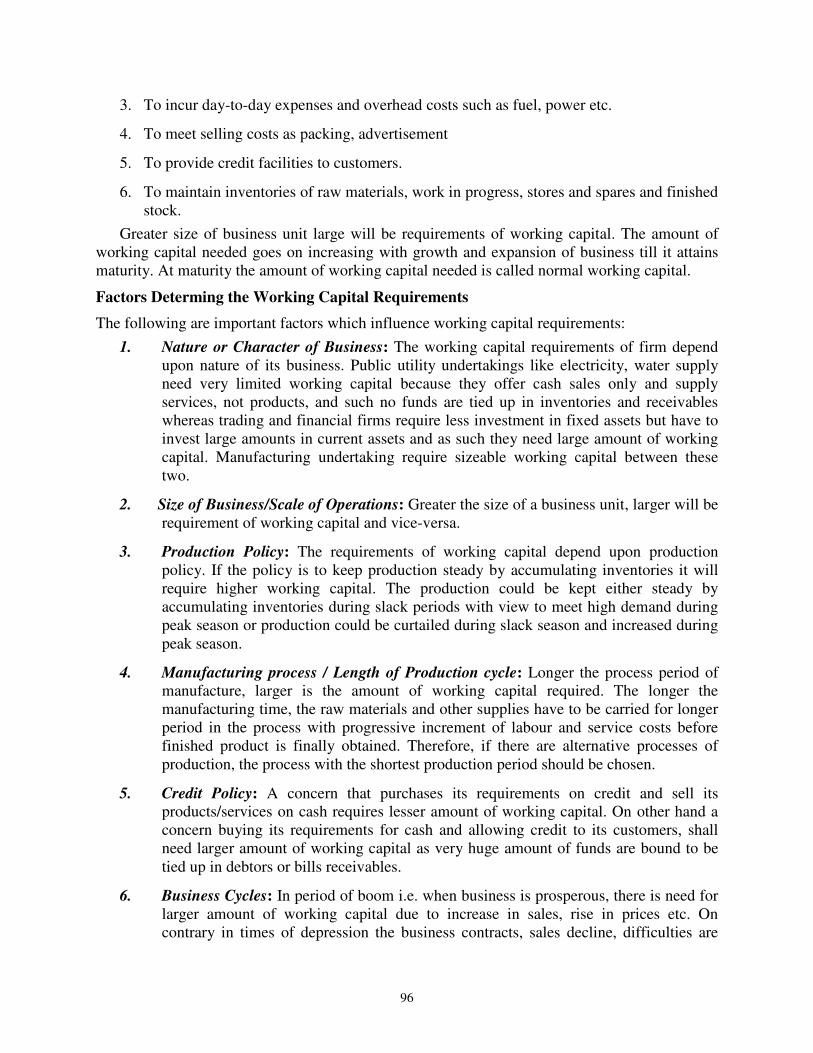
96
3. To incur day-to-day expenses and overhead costs such as fuel, power etc.
4. To meet selling costs as packing, advertisement
5. To provide credit facilities to customers.
6. To maintain inventories of raw materials, work in progress, stores and spares and finished
stock.
Greater size of business unit large will be requirements of working capital. The amount of
working capital needed goes on increasing with growth and expansion of business till it attains
maturity. At maturity the amount of working capital needed is called normal working capital.
Factors Determing the Working Capital Requirements
The following are important factors which influence working capital requirements:
1. Nature or Character of Business: The working capital requirements of firm depend
upon nature of its business. Public utility undertakings like electricity, water supply
need very limited working capital because they offer cash sales only and supply
services, not products, and such no funds are tied up in inventories and receivables
whereas trading and financial firms require less investment in fixed assets but have to
invest large amounts in current assets and as such they need large amount of working
capital. Manufacturing undertaking require sizeable working capital between these
two.
2. Size of Business/Scale of Operations: Greater the size of a business unit, larger will be
requirement of working capital and vice-versa.
3. Production Policy: The requirements of working capital depend upon production
policy. If the policy is to keep production steady by accumulating inventories it will
require higher working capital. The production could be kept either steady by
accumulating inventories during slack periods with view to meet high demand during
peak season or production could be curtailed during slack season and increased during
peak season.
4. Manufacturing process / Length of Production cycle: Longer the process period of
manufacture, larger is the amount of working capital required. The longer the
manufacturing time, the raw materials and other supplies have to be carried for longer
period in the process with progressive increment of labour and service costs before
finished product is finally obtained. Therefore, if there are alternative processes of
production, the process with the shortest production period should be chosen.
5. Credit Policy: A concern that purchases its requirements on credit and sell its
products/services on cash requires lesser amount of working capital. On other hand a
concern buying its requirements for cash and allowing credit to its customers, shall
need larger amount of working capital as very huge amount of funds are bound to be
tied up in debtors or bills receivables.
6. Business Cycles: In period of boom i.e. when business is prosperous, there is need for
larger amount of working capital due to increase in sales, rise in prices etc. On
contrary in times of depression the business contracts, sales decline, difficulties are

97
faced in collections from debtors and firms may have large amount of working capital
lying idle.
7. Rate of Growth of Business: The working capital requirements of a concern increase
with growth and expansion of its business activities. In fast growing concerns large
amount of working capital is required whereas in normal rate of expansion in the
volume of business the firm may have retained profits to provide for more working
capital.
8. Earning Capacity and Dividend Policy. The firms with high earning capacity generate
cash profits from operations and contribute to working capital. The dividend policy of
concern also influences the requirements of its working capital. A firm that maintains
a steady high rate of cash dividend irrespective of its generation of profits need more
working capital than firm that retains larger part of its profits and does not pay so high
rate of cash dividend.
9. Price Level Changes: Changes in price level affect the working capital requirements.
Generally, the rising prices will require the firm to maintain large amount of working
capital as more funds will be required to maintain the same current assets. The effect
of rising prices may be different for different firms.
10. Working Capital Cycle: In a manufacturing concern, the working capital cycle starts
with the purchase of raw material and ends with realisation of cash from the sale of
finished products. This cycle involves purchase of raw materials and stores, its
conversion into stocks of finished goods through work in progress with progressive
increment of labour and service costs, conversion of finished stock into sales, debtors
and receivables and ultimately realisation of cash and this cycle again from cash to
purchase of raw material and so on. The speed with which the working capital
completes one cycle determines the requirements of working capital longer the period
of cycle larger is requirement of working capital.
Managemant of Working Capital
Working capital refers to excess of current assets over current liabilities. Management of
working capital therefore is concerned with the problems that arise in attempting to manage
current assets, current liabilities and inter relationship that exists between them. The basic goal of
working capital management is to manage the current assets and current of a firm in such a way
that satisfactory level of working capital is maintained i.e. it is neither inadequate nor excessive.
This is so because both inadequate as well as excessive working capital positions are bad for any
business. Inadequacy of working capital may lead the firm to insolvency and excessive working
capital implies idle funds which earns no profits for the business. Working capital Management
policies of a firm have a great effect on its profitability, liquidity and structural health of
organization. In this context, evolving capital management is three dimensional in nature.
1. Dimension I is concerned with formulation of policies with regard to profitability, risk
and liquidity.
2. Dimension II is concerned with decisions about composition and level of current assets.
3. Dimension III is concerned with decisions about composition and level of current
liabilities.
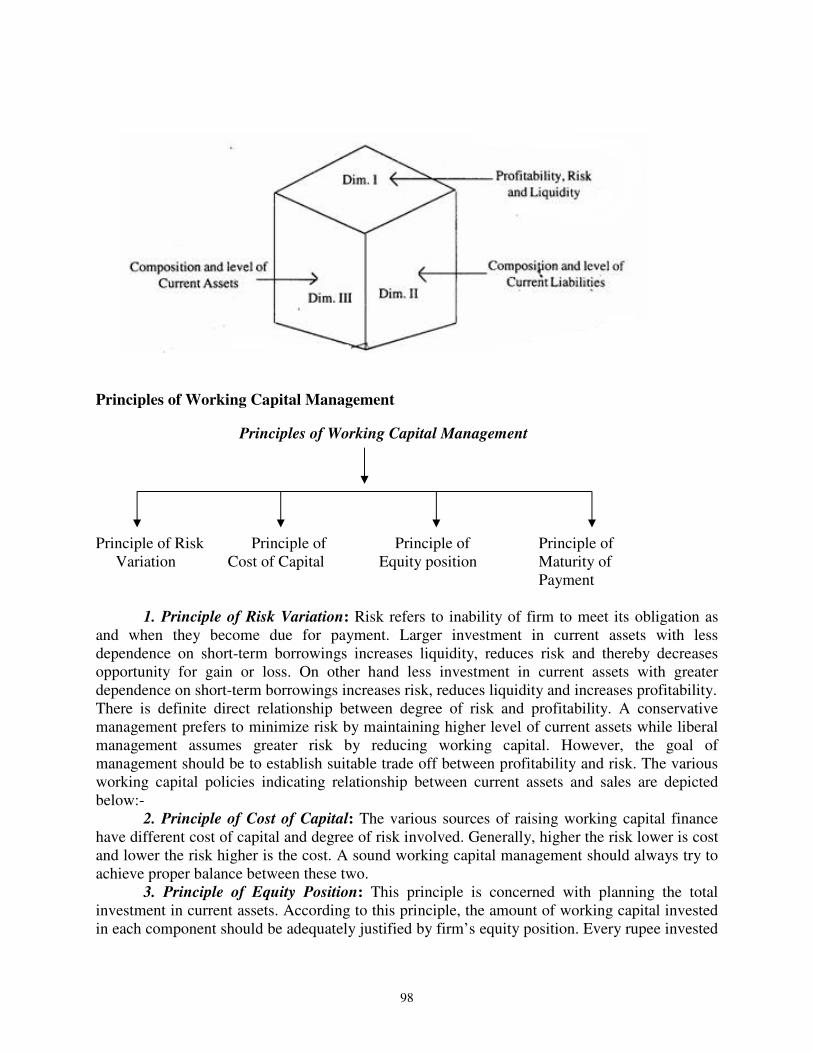
98
Principles of Working Capital Management
Principles of Working Capital Management
Principle of Risk Principle of Principle of Principle of
Variation Cost of Capital Equity position Maturity of
Payment
1. Principle of Risk Variation: Risk refers to inability of firm to meet its obligation as
and when they become due for payment. Larger investment in current assets with less
dependence on short-term borrowings increases liquidity, reduces risk and thereby decreases
opportunity for gain or loss. On other hand less investment in current assets with greater
dependence on short-term borrowings increases risk, reduces liquidity and increases profitability.
There is definite direct relationship between degree of risk and profitability. A conservative
management prefers to minimize risk by maintaining higher level of current assets while liberal
management assumes greater risk by reducing working capital. However, the goal of
management should be to establish suitable trade off between profitability and risk. The various
working capital policies indicating relationship between current assets and sales are depicted
below:-
2. Principle of Cost of Capital: The various sources of raising working capital finance
have different cost of capital and degree of risk involved. Generally, higher the risk lower is cost
and lower the risk higher is the cost. A sound working capital management should always try to
achieve proper balance between these two.
3. Principle of Equity Position: This principle is concerned with planning the total
investment in current assets. According to this principle, the amount of working capital invested
in each component should be adequately justified by firm’s equity position. Every rupee invested

99
in current assets should contribute to the net worth of firm. The level of current assets may be
measured with help of two ratios.
(i) Current assets as a percentage of total assets and
(ii) Current assets as a percentage of total sales.
4. Principle of Maturity of Payment: This principle is concerned with planning the sources
of finance for working capital. According to this principle, a firm should make every effort to
relate maturities of payment to its flow of internally generated funds. Generally, shorter the
maturity schedule of current liabilities in relation to expected cash inflows, the greater inability
to meet its obligations in time.
Determining Working Capital Financing Mix
There are three basic approaches for determining an appropriate working capital financing mix.
(1) The Hedging or Matching Approach: The term ‘hedging’ refers to two off-selling
transactions of a simultaneous but opposite nature which counterbalance effect of each other.
With reference to financing mix, the term hedging refers to ‘process of matching of
maturities of debt with maturities of financial needs’. According to this approach the maturity
of sources of funds should match the nature of assets to be financed. This approach is also
known as ‘matching approach’ which classifies the requirements of total working capital into
permanent and temporary working capital.
The hedging approach suggests that permanent working capital requirements should be
financed with funds from long-term sources while temporary working capital requirements
should be financed with short-term funds.
APPROACHES TO FINANCING
MIX
The Hedging or
Matching Approach
The Conservative
Approach
The Aggressive
Approach

100
(2) The Conservative Approach: This approach suggests that the entire estimated investments in
current assets should be financed from long-term sources and short-term sources should be used
only for emergency requirements. The distinct features of this approach are:
(ii) Liquidity is greater
(iii) Risk is minimised
(iv) The cost of financing is relatively more as interest has to be paid even on
seasonal requirements for entire period.
Trade off Between the Hedging and Conservative Approaches
The hedging approach implies low cost, high profit and high risk while the conservative
approach leads to high cost, low profits and low risk. Both the approaches are the two extremes
and neither of them serves the purpose of efficient working capital management. A trade off
between the two will then be an acceptable approach. The level of trade off may differ from case
to case depending upon the perception of risk by the persons involved in financial decision
making. However, one way of determining the trade off is by finding the average of maximum
and the minimum requirements of current assets. The average requirements so calculated may be
financed out of long-term funds and excess over the average from short-term funds.
(3). Aggressive Approach: The aggressive approach suggests that entire estimated
requirements of current asset should be financed from short-term sources even a part of fixed
assets investments be financed from short-term sources. This approach makes the finance – mix
more risky, less costly and more profitable.
Hedging Vs Conservative Approach
Hedging Approach Conservative Approach
1. The cost of financing is reduced. 1. The cost of financing is higher
2. The investment in net working
capital is nil.
2. Large Investment is blocked in
temporary working capital.
3. Frequent efforts are required to
arrange funds.
3. The firm does not face frequent
financing problems.
4. The risk is increased as firm is
vulnerable to sudden shocks.
4. It is less risky and firm is able to
absorb shocks.
Lets Sum Up
� The term working capital may be used to denote either the gross working capital which
refers to total current assets or net working capital which refers to excess of current asset
over current liabilities.
� The working capital requirement for a firm depends upon several factors such as Nature
or Character of Business, Credit Policy, Price level changes, business cycles,
manufacturing process, production policy.
� The working capital need of the firm may be bifurcated into permanent and temporary
working capital.

101
� The Hedging Approach says that permanent requirement should be financed by long term
sources while the temporary requirement should be financed by short-term sources of
finance. The Conservative approach on the other hand says that the working capital
requirement be financed from long-term sources. The Aggressive approach says that even
a part of permanent requirement may be financed out of short-term funds.
� Every firm must monitor the working capital position and for this purpose certain
accounting ratios may be calculated.
QUESTIONS
1. Explain various factors influencing working capital?
2. What are the advantages of adequate working capital?
3. Discuss various approaches to determine an appropriate financing mix of working capital?

102
12
WORKING CAPITAL: ESTIMATION AND CALCULATION
Smriti Chawla
Shri Ram College of Commerce
University of Delhi
Delhi
Estimate of Working Capital Requirements
“ Working Capital is the life blood and controlling nerve centre of a business.” No business
can be successfully run without an adequate amount of working capital. To avoid the
shortage of working capital at once, an estimate of working capital requirements should be
made in advance so that arrangements can be made to procure adequate working capital. But
estimation of working capital requirements is not an easy task and large numbers of factors
have to be considered before starting this exercise. There are different approaches available
to estimate the working capital requirements of a firm which are as follows:
(1) Working Capital as a Percentage of Net Sales: This approach to estimate the
working capital requirement is based on the fact that the working capital for any firm is directly
related to the sales volume of that firm. So, the working capital requirement is expressed as a
percentage of expected sales for a particular period. This approach is based on the assumption
that higher the sales level, the greater would be the need for working capital. There are three
steps involved in the estimation of working capital.
CHAPTER OBJECTIVES
� Estimate of Working Capital
Requirements (a) Working Capital as % of net sales (b) Working Capital as % of total assets
or fixed assets (c) Working capital based on operating
Cycle
� Illustrations

103
a) To estimate total current assets as a % of estimated net sales.
b) To estimate current liabilities as a % of estimated net sales, and
c) The difference between the two above, is the net working capital as a % of net sales.
(2) Working Capital as a Percentage of Total Assets or Fixed Asset: This approach of
estimation of working capital requirement is based on the fact that the total assets of the firm are
consisting of fixed assets and current assets. On the basis of past experience, a relationship
between (i) total current assets i.e., gross working capital; or net working capital i.e. Current
assets – Current liabilities; and (ii) total fixed assets or total assets of the firm is established. The
estimation of working capital therefore, depends upon the estimation of fixed capital which
depends upon the capital budgeting decisions.
Both the above approaches to the estimation of working capital requirement are simple in
approach but difficult in calculation.
(3) Working Capital based on Operating Cycle: In this approach, the working capital
estimate depends upon the operating cycle of the firm. A detailed analysis is made for each
component of working capital and estimation is made for each of these components. The
different components of working capital may be enumerable as follows:
Current Assets Current Liabilities
Cash and Bank Balance Creditors for Purchases
Inventory of Raw Material Creditors for Expenses
Inventory of Work-in-Progress
Inventory of Finished Goods
For manufacturing organisation, the following factors have to be taken into consideration while
making an estimate of working capital requirements.

104
From the total amount blocked in current assets estimated on the basis of the first seven
items given above, the total of the current liabilities i.e. the last two item, is deducted to find out
the requirements of working capital. In case of purely trading concern, points 1,2,3 would not
arise but all other factors from points 4 to 9 are to be taken into consideration. In order to provide
for contingencies, some extras amount generally calculated as a fixed percentage of the working
capital may be added as margin of safety.
Suggested Proforma for estimation of working capital requirements under operating cycle
is given below:
Estimation of Working Capital Requirements
I. Current Assets: Amount Amount Amount
Minimum Cash Balance ****
Inventories:
Raw Materials ****
Work-in-Progress ****
Finished Goods **** ****
Receivables
Debtors ****
Bills **** ****
Gross Working Capital (CA) **** ****
Factors Requiring Consideration While Estimating Working Capital
1. Total costs incurred on material, wages and overheads
2. The length of time for which raw material are to remain in stores before they are issued
for production.
3. The length of production cycle or work in process i.e. the time taken for conversion of
raw material into finished goods.
4. The length of sales cycle during which finished goods are to be kept waiting for sales.
5. The average period of credit allowed to customers.
6. The amount of cash required to pay day to day expenses of the business.
7. The average amount of cash required to make advance payments, if any.
8. The average credit period expected to be allowed by suppliers.
9. Time lag in the payment of wages and other expenses.

105
II. Current Liabilities : Amount Amount
Creditors for purchases ****
Creditors for Wages ****
Creditors for Overheads ****
Total Current Liabilities (CL) **** ****
Excess of CA over CL ****
+ Safety Margin ****
Net Working Capital ****
Illustration 1: XYZ Ltd. has obtained the following data concerning the average working
capital cycle for other companies in the same industry :
Raw material stock turnover 20 Days
Credit received 40 Days
Work-in-Progress Turnover 15 Days
Finished goods stock turnover 40 Days
Debtors' collection period 60 Days
95 Days
Using the following data, calculate the current working capital cycle for XYZ Ltd. And briefly
comment on it.
(Rs. in '000)
Sales 3,000
Cost of Production 2,100
Purchase 600
Average raw material stock 80
Average work-in-progress 85
Average finished goods stock 180
Average creditors 90
Average debtors 350

106
Solution: Operating cycle of XYZ Ltd.
1. Raw material
365600
80365
Material Raw Total
Material Raw Average×=×= = 49 Days
2. Work-in-progress
365100,2
85365
Production ofCost Total
progtress-in- WorkAverage×=×= = 15 Days
3. Finished Goods
3652,100
180 365
Production ofCost Total
Stock Average×=×= = 31 Days
4. Debtors
365000,3
350365
SalesCredit Total
Debtors Average×=×= = 43 Days
5. Creditors
36560
90365
Purchases Total
Creditors Average×=×= = 55 Days
Net Operating Cycle = 49 days + 15 days + 31 days + 43 days – 55 days
= 138 Days – 55 Days = 83 Days
Comment : For XYZ Ltd., the working capital cycle is below the industry average,
including a lower investment in net current assets. However, the following points should be
noted about the individual elements of working capital.
a) The stock of raw materials is considerably higher than average. So there is a need for stock
control procedure to be reviewed.
b) The value of creditors is also above average; this indicates that XYZ Ltd. is delaying the
payment of creditors beyond the credit period. Although this is an additional source of
finance, it may result in a higher cost of raw materials or loss of goodwill among the
suppliers.
c) The finished goods stock is below average. This may be due to a high demand for the firm's
goods or to efficient stock control. A low finished goods stock can, however, reduce sales
since it can cause delivery delays.
d) Debts are collected more quickly than average. The company might have employed good
credit control procedure or offer cash discounts for early payments.

107
Illustration 2: From the following data, compute the duration of operating cycle for each of
the two years and comment on the increase/decrease:
Year 1 Year 2
Stock:
Raw materials 20,000 27,000
Work-in-progress 14,000 18,000
Finished goods 21,000 24,000
Purchases 96,000 1,35,000
Cost of goods sold 1,40,000 1,80,000
Sales 1,60,000 2,00,000
Debtors 32,000 50,000
Creditors 16,000 18,000
Assume 350 Days per year for computational purposes
Solution:
a) Calculation of Operating Cycle
Year 1 Year 2
1. Raw Material Stock 20/96 x 360 = 75 Days 27/135 x 360 = 72 Days
(Average Raw Material/Total Purchase x 360)
2. Creditors period 16/96 x 360 = 60 days 18/135 x 360 = 48 days
(Average Creditor/Total Purchase) x 360
3. Work-in-progress 14/140 x 360 = 36 days 18/180 x 360 = 36 days
(Average Work-in-progress/Total cost of goods sold) x 360
4. Finished goods 21/140 x 360 = 54 days 24/180 x 360 = 48 days
(Average Finished goods/Total cost of goods sold) x 360
5. Debtors 32/160 x 360 = 72 days 50/200 x 360 = 90 days
(Average Debtors/Total Sales) x 360
Net operating cycle 177 days 198 days

108
This is an increase in length of operating cycle by 21 days i.e., 12% increase approximately.
Reasons for increase are as follows:
Debtors taking longer time to pay (90-72) 18 days
Creditors receiving payment earlier (60-48) 12 days
30 days
-- Finished goods turnover lowered (54-48) 6 days
--Raw material stock turnover lowered (75-72) 3 days
Increase in Operating Cycle 21 days
Illustration 3: A proforma cost sheet of a company provides the following particulars:
Elements of Cost
Material 40%
Direct Labour 20%
Overheads 20%
The following further particulars are available:
(a) It is proposed to maintain a level of activity of 2,00,000 units.
(b) Selling price is Rs.12/- per unit.
(c) Raw materials are expected to remain in stores for an average period of one month.
(d) Materials will be in process, on averages half a month.
(e) Finished goods are required to be in stock for an average period of one month.
(f) Credit allowed to debtors is two months.
(g) Creditor allowed by suppliers is one month.
You may assume that sales and production follow a consistent pattern.
You are required to prepare a statement of working capital requirements, a forecast Profit
and Loss Account and Balance Sheet of the company assuming that:
Rs.
Share Capital 15,00,000
8% Debentures 2,00,000
Fixed Assets 13,00,000

109
Solution:
Statement of Working Capital
Current Assets: Rs. Rs.
Stock of Raw Materials (1 month)
12100
40000,00,24
×
×
80,000
Work in progress (1/2 month):
Materials 2
1
12100
40000,00,24×
×
×
40,000
Labour 2
1
12100
20000,00,24×
×
×
20,000
Overheads 2
1
12100
20000,00,24×
×
×
20,000 80,000
Stock of Finished Goods (1 month)
Materials 12100
40000,00,24
×
×
80,000
Labour 12100
20000,00,24
×
×
40,000
Overheads 12100
20000,00,24
×
×
40,000
1,60,000
Debtors (2 months)
at cost
Material 1,60,000
Labour 80,000
Overheads 80,000 3,20,000
6,40,000
Less: Current Liabilities:
Creditors (1 month) for raw materials
12100
40000,00,24
×
×
80,000
Net Working Capital Required: 5,60,000

110
(Note: Sales = 2,00,000 × 12 = Rs.24,00,000)
Forecast Profit and Loss Account
For the year ended….
Rs. Rs.
To Materials 9,60,000 By Cost of good old 19,20,000
To Wages 4,80,000
To Overheads 4,80,000
19,20,000 19,20,000
To Cost of goods sold 19,20,000 By Sales 24,00,000
To Gross profit c/d 4,80,000
24,00,000 24,00,000
To Interest on Debentures 16,000 By Gross Profit b/d 4,80,000
To Net Profit 4,64,000
4,80,000 4,80,000
Forecast Balance Sheet
as at……
Liabilities Rs. Assets Rs.
Share Capital 15,00,000 Fixed Assets 13,00,000
8% Debentures 2,00,000 Stocks:
Net Profit 4,64,000 Raw Materials 80,000
Creditors 80,000 Work-in-Progress 80,000
Finished Goods 1,60,000
Debtors 4,00,000
Cash & Bank Balance
(Balancing figure) 2,24,000
22,44,000 22,44,000

111
Working Notes:
(a) Profits have been ignored while preparing working capital requirements for the following
reasons:
(i) Profits may or may not be used for working capital.
(ii) Even if profits have to be used for working capital, they have to be reduced by the
amount of income tax, dividends, etc.
(b) Interest on debentures has been assumed to have been paid.
Illustration 4: A proforma cost sheet of a company provides the following particulars:
Elements of Cost Amount per unit
Rs.
Raw Material 80
Direct Labour 30
Overheads 60
Total Cost 170
Profit 30
Selling Price 200
The following further particulars are available:
Raw materials are in stock on an average for one month. Materials are in process on an
average for half a month. Finished goods are in stock on an average for one month. Credit
allowed by suppliers is one month. Credit allowed to customers is two months. Lag in payment
of wages is 1½ weeks. Lag in payment of overhead expenses is one month. One-fourth of the
output is sold against cash. Cash in hand and at bank is expected to be Rs.25,000.
You are required to prepare a statement showing the working capital needed to finance a
level of activity of 1,04,000 units of production.
You may assume that production is carried on evenly throughout the year, wages and
overheads accrue similarly and a time period of 4 weeks is equivalent to a month.

112
Solution:
Statement Showing the Working Capital Needed
Current Assets Rs.
Minimum cash balance 25,000
(i) Stock of raw materials (4 weeks)
1,60,000 x 4 6,40,000
Rs.
(ii) Work-in-Process (2 weeks):
Raw materials 1,60,000 x 2 3,20,000
Direct Labour 60,000 x 2 1,20,000
Overheads 1,20,000 x 2 2,40,000 6,80,000
(iii) Stock of Finished goods (4 weeks):
Raw Materials 1,60,000 x 4 6,40,000
Direct Labour 60,000 x 4 2,40,000
Overheads 1,20,000 x 4 4,80,000 13,60,000
(iv) Sundry Debtors (8 weeks):
Raw materials 1,60,000 x 3/4 x 8 9,60,000
Direct Labour 60,000 x 3/4 x 8 3,60,000
Overheads 1,20,000 x 3/4 x 8 7,20,000 20,40,000
47,45,000
Less Current Liabilities:
(i) Sundry Creditors (4 weeks)
1,60,000 x 4 6,40,000
(ii) Wages outstanding (1-1/2 weeks): 60,000 x 2
3
90,000
(iii) Lag in payment of overheads (4 weeks)
1,20,000 x 4 4,80,000 12,10,000
Net Working Capital Needed 35,35,000

113
Working Notes:
(i) It has been assumed that a time period of 4 weeks is equivalent to one month.
(ii) It has been assumed that direct labour and overheads are in process, on average, half a
month.
(iii) Profit has been ignored and debtors have been taken at cost.
(iv) Weekly calculations have been made as follows:
(a) Weekly average of raw materials = 1,04,000 x 80/52 = 1,60,000
(b) Weekly labour cost = 1,04,000 x 30/52 = 60,000
(c) Weekly Overheads = 1,04,000 x 60/52 = 1,20,000
Illustration 5: From the following information you are required to estimate the net working
capital:
Cost per unit
Rs.
Raw Materials 400
Direct labour 150
Overheads (excluding depreciation) 300
Total Cost 850
Additional Information: 30
Selling-Price Rs.1,000 per unit
Output 52,000 units per annum
Raw Material in stock average 4 weeks
Work-in-process:
(assume 50% completion stage with
full material consumption) average 2 weeks
Finished goods in stock average 4 weeks
Credit allowed by suppliers average 4 weeks
Credit allowed to debtors average 8 weeks
Cash at bank is expected to be Rs.50,000
Assume that production is sustained at an even pace during the 52 weeks of the year. All sales
are on credit basis. State any other assumption that you might have made while computing.

114
Solution :
Statement Showing Net Working Capital Requirements
Current Assets : Rs.
Minimum cash balance 50,000
Stock of Raw Materials (4 weeks)
52,000 x 400 x 52
4
16,00,000
Stock of work-in-progress (2 weeks)
Raw material 52,000 x 400 x 52
2
8,00,000
Direct labour (50% completion)
52,000 x 150 x 100
50x
52
2
1,50,000
Overheads (50% completion)
52,000 x 300 x 100
50x
52
2
3,00,000 12,50,000
Stock of Finished goods (4 weeks)
52,000 x 850 x 52
4
34,00,000
Amount blocked in Debtors at cost (8 weeks)
52,000 x 850 x 52
8
68,00,000
Total Current Assets 1,31,00,000
Less: Current Liabilities:
Creditors for raw materials (4 weeks)
52,00,000 x 400 x 52
4
16,00,000
Net Working Capital Required 1,15,00,000
Illustration 6: Texas Manufacturing Company Ltd. is to start production on 1st January,
1995. The prime cost of a unit is expected to be Rs.40 out of which Rs.16 is for materials and
Rs.24 for labour. In addition, variable expenses per unit are expected to be Rs.8 and fixed
expenses per month Rs.30,000. Payment for materials is to be made in the month following the
purchases. One-third of sales will be for cash and the rest on credit for settlement in the
following month. Expenses are payable in the month in which they are incurred. The selling
price is fixed at Rs.80 per unit. The number of units manufactured and sold are expected to be as
under:
January 900
February 1,200
March 1,800
April 2,100
May 2,100
June 2,400

115
Draw up a statement showing requirements of working capital from month to month, ignoring
the question of stocks.
Solution:
Statement Showing Requirement of Working Capital
Januar
y Rs.
Februa
ry Rs.
March
Rs.
April Rs. May Rs. June Rs.
Payments:
Materials - 14,400 19,200 28,800 33,600 33,600
Wages 21,600 28,800 43,200 50,400 50,400 57,600
Fixed Expenses 30,000 30,000 30,000 30,000 30,000 30,000
Variable Expenses 7,200 9,600 14,400 16,800 16,800 19,200
58,800 82,800 1,06,800 1,26,000 1,30,800 1,40,400
Receipts:
Cash Sales 24,000 32,000 48,000 56,000 56,000 64,000
Debtors - 48,000 64,000 96,000 1,12,000 1,12,000
24,000 80,000 1,12,000 1,52,000 1,68,000 1,76,000
Working Capital Required
Payments-Receipts)
34,800 2,800 - - - -
Surplus - - 5,200 26,000 37,200 35,600
Cumulative Requirements
of Working Capital
34,800 37,600 32,400 6,400 - -
Surplus Working Capital - - - - 30,800 66,400
Working Notes:
(i) As payment for material is made in the month following the purchase, there is no
payment for material in January. In February, material payment is calculated as 900 x 16
= Rs.14,400 and in the same manner for other months.
(ii) Cash sales are calculated as:
For January 900 x 80 x 1/3 = Rs.24,000 and in the same manner for other months.
(iii) Receipts from debtors are calculated as:
For Jan. – Nil because cash from debtors is collected in the month following the sales.
For Feb. – 900 x 80 x 2/3 = Rs.48,000
For March – 12002 x 80 x 2/3 = Rs.64,000, and so on.

116
3
FINANCING OF WORKING CAPITAL
Smriti Chawla Shri Ram College of Commerce
University of Delhi Delhi
Introduction
The working capital requirements of concern can be classified as:
(a)Permanent or Fixed working capital requirements
(b)Temporary or Variable working capital requirements
In any concern, a part of the working capital investments are as permanent investments in
fixed assets. This is so because there is always a minimum level of current asses which are
continuously required by enterprise to carry out its day-to-day business operations and this
minimum cannot be expected to reduce at any time. This minimum level of current assets give
rise to permanent or fixed working capital as this part of working capital is permanently blocked
in current assets.
Similarly, some amount of working capital may be required to meet the seasonal
demands and some special exigencies such as rise in prices, strikes etc. this proportion of
working capital gives rise to temporary or variable working capital which cannot be permanently
employed gainfully in business.
The fixed proportion of working capital should be generally financed from the fixed
capital sources while temporary or variable working capital requirements of a concern may be
met from the short-term sources of capital.
CHAPTER OBJECTIVES
� Introduction
� Financing of Permanent/Fixed or Long term Working Capital
� Financing of Temporary or Short term
Working Capital � New Trends in Financing Working Capital by
banks � Lets Sum Up
� Questions
117
The various sources for financing of working capital are as follows:
Sources of Working Capital
Permanent or Fixed Temporary or Variable
1. Shares
2. Debentures
3. Public deposits
4. Ploughing back of profits
5. Loans from Financial Institutions.
1. Trade Credit
2. Accrued Expenses
3. Commercial Paper
4. Factoring or Accounts
Receivable Credit
5. Instalment Credit
6. Commercial Banks
Financing of Permanent/Fixed or Long-Term Working Capital
Permanent working capital should be financed in such a manner that the enterprise may
have its uninterrupted use for a sufficiently long period. There are five important sources of
permanent or long-term working capital.
(a) Shares: Issue of shares is the most important source for raising the permanent or long-
term capital. A company can issue various types of shares as equity shares, preference shares and
deferred shares. According to the Companies Act, 1956, however, a public company cannot issue
deferred shares. Preference shares carry preferential rights in respect of dividend at a fixed rate
and in regard to the repayment of capital at the time of winding up the company. Equity shares
do not have any fixed commitment charge and the dividend on these shares is to be paid subject
to the availability of sufficient profits. As far as possible, a company should raise the maximum
amount of permanent capital by the issue of shares.
(b) Debentures: A debenture is an instrument issued by the company acknowledging its
debt to its holder. It is also an important method of raising long-term or permanent working
capital. The debenture-holders are the creditors of the company. A fixed rate of interest is paid
on debentures. The interest on debentures is a charge against profit and loss account. The
debentures are generally given floating charge on the assets of the company. When the
debentures are secured they are paid on priority to other creditors. The debentures may be of
various kinds such as simple, naked or unsecured debentures, secured or mortgaged debentures,
redeemable debentures, irredeemable debentures, convertible debentures and non-convertible
debenture. The firm issuing debentures also enjoys a number of benefits such as trading on
equity, retention of control, tax benefits, etc.
(c) Public Deposits : Public deposits are the fixed deposits accepted by a business
enterprise directly from the public. This source of raising short term and medium term finance
was very popular in the absence of banking facilities. Public deposits as a source of finance have
a large number of advantages such as very simple and convenient source of finance, taxation
benefits, trading on equity, no need of securities and an inexpensive source of finance. But it is

118
not free from certain dangers such as, it is uncertain, unreliable, unsound and inelastic source of
finance. The Reserve Bank of India has also laid down certain limits on public deposits.
(iv) Ploughing back of profits: Ploughing back of profits means the reinvestments by
concern of its surplus earnings in its business. It is an internal source of finance and is most
suitable for an established firm for its expansion, modernisation and replacement etc. This
method of finance has a number of advantages as it is the cheapest rather cost-free source of
finance; there is no need to keep securities; there is no dilution of control; it ensures stable
dividend policy and gains confidence of the public. But excessive resort to ploughing back of
profits may lead to monopolies, misuse of funds, over capitalization and speculation etc.
(v) Loans from Financial Institutions: Financial institutions such as Commercial Banks,
Life Insurance Corporation, Industrial Finance Corporation of India, State financial
Corporations, State Industrial Development Corporations, Industrial Development Bank of India,
etc. also provide short-term, medium-term and long-term loans. This source of finance is more
suitable to meet the medium term demands of working capital. Interest is charged on such loans
at a fixed rate and the amount of the loan is to be repaid by way of instalments in a number of
years.
Financing of Temporary, Variable or Short Term Working Capital
1. Trade Credit: Trade credit refers to the credit extended by the suppliers of goods in the
normal course of business. As present day commerce is built upon credit, the trade credit
arrangement of a firm with its suppliers is an important source of short-term finance. The credit-
worthiness of a firm and the confidence of its suppliers are the main basis of securing trade
credit. It is mostly granted on an open account basis whereby supplier sends goods to the buyer
for the payment to be received in future as per terms of the sales invoice. It may also take the
form of bills payable whereby the buyer signs a bill of exchange payable on a specified future
date.
When a firm delays the payment beyond the due date as per the terms of sales invoice, it
is called stretching accounts payable. A firm may generate additional short-term finances by
stretching accounts payable, but it may have to pay penal interest charges as well as to forgo cash
discount. If a firm delays the payment frequently, it adversely affects the credit worthiness of the
firm and it may not be allowed such credit facilities in future.
The main advantages of trade credit as a source of short-term finance include:
(i) It is an easy and convenient method of finance.
(ii) It is flexible as the credit increases with the growth of the firm.
(iii)It is informal and spontaneous source of finance.
However, the biggest disadvantage of this method of finance is charging of higher prices by the
suppliers and loss of cash discount.
2. Accrued Expenses: Accrued expenses are the expenses which have been incurred but
not yet due and hence not yet paid also. These simply represent a liability that a firm has to pay
for the services already received by it. The most important item of accruals are wages and
salaries, interest and taxes. The longer the payment period of wages and salaries the greater is the
amount of liability towards employees. In same manner, accrued interest and taxes also
constitute a short-term source of finance.

119
3. Commercial Paper: Commercial paper represents unsecured promissory notes issued
by firms to raise short-term funds. It is an important money market instrument in advanced
countries like U.S.A. In India, the Reserve Bank of India introduced commercial paper in the
Indian money market on the recommendations of the Working Group on Money Market (Vaghul
Committee). But only large companies enjoying high credit rating and sound financial health can
issue commercial paper to raise short-term funds. The Reserve Bank of India has laid down a
number of conditions to determine eligibility of a company for the issue of commercial paper.
Only a company which is listed on the stock exchange, has a net worth of at least Rs. 10 crores
and a maximum permissible bank finance of Rs. 25 crores can issue commercial paper not
exceeding 30 per cent of its working capital limit.
The maturity period of commercial paper, in India, mostly ranges from 91 to 180 days. It
is sold at a discount from its face value and redeemed at face value on its maturity. Hence the
cost of raising funds, through this source, is a function of the amount of discount and the period
of maturity and no interest rate is provided by the Reserve Bank of India for this purpose.
Commercial paper is usually bought by investors including banks, insurance companies, unit
trusts and firms to invest surplus funds for a short-period. A credit rating agency called CRISIL,
has been set up in India by ICICI and UTI to rate commercial paper.
Commercial paper is a cheaper source of raising short-term finance as compared to the
bank credit and proves to be effective even during period of tight bank credit. However, it can be
used as a source of finance only by large companies enjoying high credit rating and sound
financial health. Another disadvantage of commercial paper is that it cannot be redeemed before
the maturity date even if the issuing firm has surplus funds to pay back.
4. Factoring or Accounts Receivable Credit: Another method of raising short-term
finance is through accounts receivable credit offered by commercial banks and factors. A
commercial bank provide finance by discounting the bills. Thus, a firm gets immediate payment
for sales made on credit. A factor is a financial institution which offer services relating to
management and financing of debts arising out of credit sales.
5. Instalment Credit: This is another method by which the assets are purchased and the
possession of goods is taken immediately but payment is made in instalments over a pre-
determined period of time. Generally, interest is charged on the unpaid price or it may be
adjusted in the price.. But in any case it provides funds for sometime and is used as a source of
short-term working capital by many business houses which have difficult fund position.
Working Capital Finance by Commercial Banks
Commercial banks are the most important source of short-term capital. The major portion of
working capital loans are provided by commercial banks. They provide a wide variety of loans
tailored to meet the specific requirements of a concern. The different forms in which the banks
normally provide loans and advances are as follows:
(a) Loans
(b) Cash Credits
(c) Overdrafts
(d) Purchasing and Discounting of bills.
(a) Loans: When a bank makes an advance in lump-sum against some security it is called
a loan, In case of a loan, a specified amount is sanctioned by the bank to the customer. The entire

120
loan amount is paid to the borrower either in cash or by credit to his account. The borrower is
required to pay interest on the entire amount of the loan from the date of the sanction. A loan
may be repayable in lump sum or installments, Interest on loans is calculated at quarterly rests
and where repayments are stipulated in instalments, the interest is calculated at quarterly rests on
the reduced balances. Commercial banks generally provide short-term loans up to one year for
meeting working capital requirements. But now-a-days term loans exceeding one year are also
provided by banks. The term loans may be either medium-term or long-term loans.
(b) Cash Credits: A cash credit is an arrangement by which a bank allows his customer to
borrow money upto a certain limit against some tangible securities or guarantees.
(c) Overdrafts: Overdrafts means an agreement with a bank by which a current account-
holder is allowed to withdraw more than the balance to his credit upto a certain limit. There are
no restrictions for operation of overdraft limits. The interest is charged on daily overdrawn
balances. The main difference between cash credit and overdraft is that overdraft is allowed for a
short period and is a temporary accommodation whereas the cash credit is allowed for a longer
period. Overdraft accounts can either be clean overdrafts, partly secured or fully secured.
(d) Purchasing and Discounting of Bills: Purchasing and discounting of bills is the
most important form in which a bank lends without any collateral security. Present day
commerce is built upon credit. The seller draws a bill of exchange on the buyer of goods on
credit. Such a bill may be either a clean bill or a documentary bill which is accompanied by
documents of title to goods such as a railway receipt. The bank purchases the bills payable on
demand and credits the customer's account with the amount of bill less discount. At the maturity
of the bills, bank presents the bill to its acceptor for payment. In case the bill discounted is
dishonoured by non-payment, the bank recovers the full amount of the bill from the customer
along with expenses in that connection.
In addition to the above mentioned forms of direct finance, commercial banks help their
customers in obtaining credit from their suppliers through the letter of credit arrangement.
Letter of Credit
A letter or credit popularly known as L/c is an undertaking by a bank to honour the
obligations of its customer upto a specified amount, should the customer fail to do so. It helps its
customers to obtain credit from suppliers because it ensures that there is no risk of non-payment.
L/c is simply a guarantee by the bank to the suppliers that their bills upto a specified amount
would be honoured. In case the customer fails to pay the amount, on the due date, to its suppliers,
the bank assumes the liability of its customer for the purchases made under the letter of credit
arrangement.
A letter of credit may be of many types, such as:
(i) Clean Letter of Credit. It is a guarantee for the acceptance and payment of bills
without any conditions.
(ii) Documentary Letter of Credit. It requires that the exporter’s bill of exchange be
accompanied by certain documents evidencing title to the goods.
(iii) Revocable Letter of Credit. It is one which can be withdrawn by the issuing bank
without the prior consent of the exporter.
(iv) Irrevocable Letter of Credit:. It cannot be withdrawn without the Consent of the
beneficiary.

121
(v) Revolving Letter of Credit. In such type of letter of credit the amount of credit it
automatically reversed to the original amount after such an amount has once been paid as per
defined conditions of the business transaction. There is no deed for further application for
another letter of credit to be issued provided the conditions specified in the first credit are
fulfilled.
(vi) Fixed Letter of Credit. It fixes the amount of financial obligation of the issuing bank
either in one bill or in several bills put together.
Security Required in Bank Finance
Banks usually do not provide working capital finance without obtaining adequate security.
The following are the most important modes of security required by a bank:
1. Hypothecation: Under this arrangement, bank provides working capital finance against
the security of movable property, usually inventories. The borrower does not give possession of
the property to the bank. It remains with the borrower and hypothecation is merely a charge
against property for the amount of debt. If the borrower fails to pay his dues to the bank, the
banker may file a case to realise his dues by sales of the goods/property hypothecated.
2. Pledge: Under this arrangement, the borrower is required to transfer the physical
possession of the property or goods to the bank as security. The bank will have the right of lien
and can retain the possession of goods unless the claim of the bank is met. In case of default, the
bank can even sell the goods after giving due notice.
3. Mortgage: In addition to the hypothecation or pledge, banks usually ask for mortgages as
collateral or additional security. Mortgage is the transfer of a legal or equitable interest in a
specific immovable property for the payment of a debt. Although, the possession of the property
remains with the borrower, the full legal title is transferred to the lender. In case of default, the
bank can obtain decree from the court to sell the immovable property mortgaged so as to realise
its dues.
New Trend in Financing Working Capital by Banks: Dehejia Committee Report
National Credit Council constituted a committee under the chairmanship of
Shri V.T. Dehejia in 1968 to ‘determine the extent to which credit needs of industry and trade
are likely to be inflated and how such trends could be checked’ and to go into establishing some
norms for lending operations by commercial banks. The committee was of the opinion that there
was also a tendency to divert short-term credit for long-term assets. Although committee was of
the opinion that it was difficult to evolve norms for lending to industrial concerns, the committee
recommended that the banks should finance industry on the basis of a study of borrower’s total
operations rather than security basis alone. The Committee further recommended that the total
credit requirements of the borrower should be segregated into ‘Hard Core’ and ‘Short-term’
component. The ‘Hard Core’ component which should represent the minimum level of
inventories which the industry was required to hold for maintaining a given level of production
should be put on a formal term loan basis and subject to repayment schedule. The committee was
also of the opinion that generally a customer should be required to confine his dealings to one
bank only.
� Tandon Committee Report
Reserve Bank of India set up a committee under the chairmanship of Shri P.L. Tandon in
July 1974. The terms of reference of the Committee were:

122
1. To suggest guidelines for commercial banks to follow up and supervise credit from the
point of view of ensuring proper end use of funds and keeping a watch on the safety of
advances;
2. To suggest the type of operational data and other information that may be obtained by
banks periodically from the borrowers and by the Reserve Bank of India from the leading
banks;
3. To make suggestions for prescribing inventory norms for the different industries, both in
the private and public sectors and indicate the broad criteria for deviating from these
norms;
4. To make recommendations regarding resources for financing the minimum working
capital requirements;
5. To suggest criteria regarding satisfactory capital structure and sound financial basis in
relation to borrowings;
6. To make recommendations as to whether the existing pattern of financing working capital
requirements by cash credit/overdraft system etc., requires to be modified, if so, to
suggest suitable modifications.
The committee was of the opinion that: (i) bank credit is extended on the amount of security
available and not according to the level of operations of the customer, (ii) bank credit instead of
being taken as a supplementary to other sources of finance is treated as the first source of
finance, Although the Committee recommended the continuation of the existing cash credit
system, it suggested certain modifications so as to control the bank finance. The banks should get
the information regarding the operational plans of the customer in advance so as to carry a
realistic appraisal of such plans and the banks should also know the end-use of bank credit so
that the finances are used only for purposes for which they are lent.
The recommendations of the committee regarding lending norms have been suggested under
three alternatives. According to the first method, the borrower will have to contribute a minimum
of 25% of the working capital gap from long-term funds, i.e., owned funds and term borrowing;
this will give a minimum current ratio of 1.17 : 1. Under the second method the borrower will
have to provide a minimum of 25% of the total current assets from long-term funds; this will
give a minimum current ratio of 1.33 : 1. In the third method, the borrower's contribution from
long-term funds will be to the extent of the entire core current assets and a minimum of 25% of
the balance current assets, thus strengthening the current ratio further.
� Chore Committee Report
The Reserve Bank of India in March, 1979 appointed another committee under the
chairmanship of Shri K.B. Chore to review the working of cash credit system in recent years
with particular reference to the gap between sanctioned limits and the extent of their utilisation
and also to suggest alternative type of credit facilities which should ensure greater credit
discipline.
The important recommendations of the Committee are as follows:
(i) The banks should obtain quarterly statements in the prescribed format from all
borrowers having working capital credit limits of Rs. 50 lacs and above.
(ii) The banks should undertake a periodical review of limits of Rs. 10 lacs and above.
(iii) The banks should not bifurcate cash credit accounts into demand loan and cash credit
components.

123
(iv) If a borrower does not submit the quarterly returns in time the banks may charge
penal interest of one per cent on the total amount outstanding for the period of
default.
(v) Banks should discourage sanction of temporary limits by charging additional one per
cent interest over the normal rate on these limits.
(vi) The banks should fix separate credit limits for peak level and non-peak level,
wherever possible. .
(vii) Banks should take steps to convert cash credit limits into bill limits for financing
sales.
� Marathe Committee Report
The Reserve Bank of India, in 1982 appointed a committee under the chairmanship of
Marathe to review the working of Credit Authorisation Scheme (CAS) and suggest measures for
giving meaningful directions to the credit management function of the Reserve Bank. The
recommendations of the committee have been accepted by the Reserve Bank of India with minor
modifications.
The principal recommendations of the Marathe Committee include;
(i) The committee has declared the Third Method of Lending as suggested by the Tandon
Committee to be droped. Hence, in future, the banks would provide credit for working
capital according the Second Method of Lending.
(ii) The committee has suggested the introduction of the ‘Fast Track Scheme’ to improve the
quality of credit appraisal in Banks. It recommended that commercial banks can release
without prior approval of the Reserve Bank 50% of the additional credit required by the
borrowers (75% in case of export oriented manufacturing units) where the following
requirements are fulfilled:
(a) The estimates/projections in regard to production, sales chargeable current assets,
other current assets, current liabilities other than bank borrowings and net working
capital are reasonable in terms of the past trends and assumptions regarding most
likely trends during the future projected period.
(b) The classification of assets and liabilities as ‘current’ and ‘non-current’ is in
conformity with the guidelines issued by the Reserve Bank of India.
(c) The projected current ratio is not below 1.33:1.
(d) The borrower has been submitting quarterly information and operating statements
(Form I, II and III) for the past six months within the prescribed time and
undertakes to do the same in future also.
(e) The borrower undertakes to submit to the bank his annual account regularly and
promptly further, the bank is required to review the borrower’s facilities at least
once in a year even if the borrower does not need enhancement in credit facilities.
� Kannan Committee
The Kannan Committee was the first committee to have suggested that the prescribed
uniform formula for MPBF should go and the banks should have the sole discretion to determine
borrowing limits of corporates. However, the change from the MPBF system should keep in
view the size of various banks, their delegation system, exposure limit etc. Banks and the

124
borrowers should be left free to decide the system they adopt for financing working capital.
The main recommendations of the committee are summarized as under:
(i) The system of cash credit should be replaced by a system of loans for working
capital.
(ii) The uniform formula for MPBF should be abolished and banks should be given
discretion for determining borrowing limits for corporates.
(iii) The corporate borrowers may be allowed to issue short-term debentures for
meting short-term requirements and banks may subscribe to these debentures.
(iv) Margins and holding levels of stocks and receivables as security may be left to the
discretion of the banks.
(v) Benchmark current ratio of 1.33:1 should be left to the discretion of the banks.
(vi) A credit information bureau should be floated independently by banks.
(vii) Banks should be allowed to decide policy norms for issue of commercial papers.
(viii) Borrowers will have to obtain prior approval for investment of funds outside the
business in inter corporate deposits etc.
(ix) Banks should also try out the syndicate form of lending.
(x) Periodical statement of stocks, debtors coupled with verification of securities to
be the credit-monitoring tool.
Lets Sum up
� The total requirement of working capital may be bifurcated in permanent and
temporary working capital.
� The permanent working capital which is required irrespective of the fluctuations in
the sale level should be financed by arranging funds from long-term sources such as
debt and equity.
� However, the temporary requirement should be financed from short-term sources of
finance.
� Commercial papers as unsecured promissory note can also be used by a firm, under
the guidelines provided by the RBI, to arrange funds for a short period.
� Commercial banks also provide short-term credit in terms of cash credit, bills
purchased, letter of credit and working capital term loans.
QUESTIONS
1 Examine the importance of trade credit and accrued expenses as a source of working capital
financing?
2 Write short note on commercial paper?
3 Describe important features of Tandon Committee?

125
4
MANAGEMENT OF CASH
Smriti Chawla Shri Ram College of Commerce
University of Delhi Delhi
Introduction
Cash is one of the current assets of a business. It is needed at all times to keep the
business going. A business concern should always keep sufficient cash for meeting its
obligations. Any shortage of cash will hamper the operations of a concern and any excess
of it will be unproductive. Cash is the most unproductive of all the assets. While fixed
asses like machinery, plant, etc. and current assets such as inventory will help the
business in increasing its earning capacity, cash in hand will not add anything to the
concern. It is in this context that cash management has assumed much importance.
Nature of Cash
For some persons, cash means only money in the form of currency (cash in hand).
For other persons, cash means both cash in hand and cash at bank. Some even include
near cash assets in it. They take marketable securities too as part of cash. These are the
securities which can easily be converted into cash.
Cash itself does not produce good or services. It is used as a medium to acquire
other assets. It is the other assets which are used in manufacturing goods or providing
services. The idle cash can be deposited in bank to earn interest.
CHAPTER OBJECTIVES
� Introduction � Nature of Cash � Motives for holding Cash � Cash Management � Managing Cash Flows
o Methods of accelerating Cash Inflows o Methods of Slowing Cash Outflows
� Determining Optimum Cash Balance � Baumol’s Model � Miller-Orr Model � Investment of Surplus Funds � Illustrations � Lets Sum Up � Questions

126
A business has to keep required cash for meeting various needs. The assets
acquired by cash again help the business in producing cash. The goods manufactured of
services produced are sold to acquire cash. A firm will have to maintain a critical level of
cash. If at a time it does not have sufficient cash with it, it will have to borrow from the
market for reaching the required level.
There remains a gap between cash inflows and cash outflows. Sometimes cash
receipts are more than the payments or it may be vice-versa at another time. A financial
manager tries to synchronize the cash inflow and cash outflows.
Motives for Holding Cash
The firm’s needs for cash may be attributed to the following needs: Transactions
motive, Precautionary motive and Speculative motive. These motives are discussed as
follows:
1. Transaction Motive: A firm needs cash for making transacions in the day-to-
day operations. The cash is needed to make purchases, pay expenses, taxes, dividend, etc.
The cash needs arise due to the fact that there is no complete synchronization between
cash receipts and payments. Sometimes cash receipts exceed cash payments or vice-
versa. The transaction needs of cash can be anticipated because the expected payments in
near future can be estimated. The receipts in future may also be anticipated but the things
do not happen as desired. If more cash is needed for payments than receipts, it may be
raised through bank overdraft. On the other hand if there are more cash receipts than
payments, it may be spent on marketable securities.
2. Precautionary Motive: A firm is required to keep cash for meeting various
contingencies. Though cash inflows and cash outflows are anticipated but there may be
variations in these estimates. For example a debtor who was to pay after 7 days may
inform of his inability to pay; on the other hand a supplier who used to give credit for 15
days may not have the stock to supply or he may not be in a position to give credit at
present. In these situations cash receipts will be less then expected and cash payments
will be more as purchases may have to be made for cash instead of credit. Such
contingencies often arise in a business. A firm should keep some cash for such
contingencies or it should be in a position to raise finances at a short period.
3. Speculative Motive: The speculative motive relates to holding of cash for
investing in profitable opportunities as and when they arise. Such opportunities do not
come in a regular manner. These opportunities cannot be scientifically predicted but only
conjectures can be made about their occurrence. The price of shares and securities may
be low at a time with an expectation that these will go up shortly. Such opportunities can
be availed of if a firm has cash balance with it.
Cash Management
Cash management has assumed importance because it is the most significant of all
the current assets. It is required to meet business obligations and it is unproductive when
not used.
Cash management deals with the following:
(i) Cash inflows and outflows
(ii) Cash flows within the firm

127
(iii) Cash balances held by the firm at a point of time.
Cash Management needs strategies to deal with various facets of cash. Following are
some of its facets.
(a) Cash Planning: Cash planning is a technique to plan and control the use of
cash. A projected cash flow statement may be prepared, based on the present business
operations and anticipated future activities. The cash inflows from various sources may
be anticipated and cash outflows will determine the possible uses of cash.
(b) Cash Forecasts and Budgeting: A cash budget is the most important device
for the control of receipts and payments of cash. A cash budget is an estimate of cash
receipts and disbursements during a future period of time. It is an analysis of flow of cash
in a business over a future, short or long period of time. It is a forecast of expected cash
intake and outlay.
The short-term forecasts can be made with the help of cash flow projections. The
finance manager will make estimates of likely receipts in the near future and the expected
disbursements in that period. Though it is not possible to make exact forecasts even then
estimates of cash flow will enable the planners to make arrangement for cash needs. A
financial manager should keep in mind the sources from where he will meet short-term
needs. He should also plan for productive use of surplus cash for short periods.
The long-term cash forecasts are also essential for proper cash planning. These
estimates may be for three, four, five or more years. Long-term forecasts indicate
company’s future financial needs for working capital, capital projects, etc.
Both short term and long term cash forecasts may be made with help of following
methods.
(a) Receipts and Disbursements method
(b) Adjusted net income method
Receipts and Disbursements method
In this method the receipt and payment of cash are estimated. The cash receipts
may be from cash sales, collections from debtors, sale of fixed assets, receipts of
dividend or other income of all the items; it is difficult to forecast the sales. The sales
may be on cash as well as credit basis. Cash sales will bring receipts at the time of sales
while credit sale will bring cash later on. The collections from debtors will depend upon
the credit policy of the firm. Any fluctuation in sales will disturb the receipts of cash.
Payments may be made for cash purchases, to creditors for goods, purchase of fixed
assets etc.
The receipts and disbursements are to be equalled over a short as well as long
periods. Any shortfall in receipts will have to be met from banks or other sources.
Similarly, surplus cash may be invested in risk free marketable securities. It may be easy
to make estimates for payments but cash receipts may not be accurately made.
Adjusted Net Income Method
This method may also be known as sources and uses approach. It generally has
three sections: sources of cash, uses of cash and adjusted cash balance. The adjusted net
income method helps in projecting the company’s need for cash at some future date and
to see whether the company will be able to generate sufficient cash. If not, then it will

128
have to decide about borrowing or issuing shares etc. in preparing its statement the items
like net income, depreciation, dividends, taxes etc. can easily be determined from
company’s annual operating budget. The estimation of working capital movement
becomes difficult because items like receivables and inventories are influenced by factors
such as fluctuations in raw material costs, changing demand for company’s products.
This method helps in keeping control on working capital and anticipating financial
requirements.
Managing Cash Flows
After estimating the cash flows, efforts should be made to adhere to the estimates
or receipts and payments of cash. Cash management will be successful only if cash
collections are accelerated and cash disbursements, as far as possible, are delayed. The
following methods of cash management will help:
Methods of Accelerating Cash Inflows
1. Prompt Payment by Customers: In order to accelerate cash inflows, the
collections from customers should be prompt. This will be possible by prompt
billing. The customers should be promptly informed about the amount payable
and the time by which it should be paid. Another method for prompting customers
to pay earlier is to allow them cash discount.
2. Quick Conversion of Payment into Cash: Cash inflows can be accelerated by
improving the cash collecting process. Once the customer writes a cheque in
favour of the concern the collection can be quickened by its early collection.
There is a time gap between the cheque sent by the customer and the amount
collected against it. This is due to many factors, (i) mailing time, i.e. time taken
by post office for transferring cheque from customer to the firm, referred to as
postal float; (ii) time taken in processing the cheque within the organization and
sending it to bank for collection, it is called lethargy and (iii) collection time
within the bank, i.e. time taken by the bank in collecting the payment from the
customer’s bank, called bank float. The postal float, lethargy and bank float are
collectively referred to as deposit float. The term deposit float refers to cheques
written buy customers but the amount not yet usable by the firm.
3. Decentralised Collections: A big firm operating over wide geographical area can
accelerate collections by using the system of decentralised collections. A number
of collecting centres are opened in different areas instead of collecting receipts at
one place. The idea of opening different collecting centres is to reduce the mailing
time for customer’s dispatch of cheque and its receipt in the firm and then
reducing the time in collecting these cheques.
4. Lock Box System: Lock box system is another technique of reducing mailing,
processing and collecting time. Under this system the firm selects some collecting
centres at different places. The places are selected on the basis of number of
consumers and the remittances to be received from a particular place.
Methods of Slowing Cash Outflows
A company can keep cash by effectively controlling disbursements. The objective
of controlling cash outflows is slow down the payments as far as possible. Following
methods can be used to delay disbursements:

129
1. Paying on Last Date: The disbursements can be delayed on making payments
on the last due date only. It is credit is for 10 days then payment should be made on 10th
day only. It can help in using the money for short periods and the firm can make use of
cash discount also.
2. Payments through Drafts: A company can delay payments by issuing drafts to
the suppliers instead of giving cheques. When a cheque is issued then the company will
have to keep a balance in its account so that the cheque is paid whenever it comes. On the
other hand a draft is payable only on presentation to the issuer. The receiver will give the
draft to its bank for presenting it to the buyer’s bank. It takes a number of days before it is
actually paid. The company can economise large resources by using this method.
3. Adjusting Payroll Funds: Some economy can be exercised on payroll funds
also. It can be done by reducing the frequency of payments. If the payments are made
weekly then this period can be extended to a month. Secondly, finance manager can plan
the issuing of salary cheques and their disbursements. If the cheques are issued on
Saturday then only a few cheque may be presented for payment, even on Monday all
cheques may not be presented.
4. Centralisation of Payments: The payments should be centralised and payments
should be made through drafts or cheques. When cheques are issued from the main office
then it will take time for the cheques to be cleared through post. The benefit of cheque
collecting time is availed.
5. Inter-bank Transfer: An efficient use of cash is also possible by inter-bank
transfers. If the company has accounts with more than one bank then amounts can be
transferred to the bank where disbursements are to be made. It will help in avoiding
excess amount in one bank.
6. Making use of Float: Float is a difference between the balance shown in
company’s cash book (Bank column) and balance in passbook of the bank. Whenever a
cheque is issued, the balance at bank in cashbook is reduced. The party to whom the
cheque is issued may not present it for payment immediately. If the party is at some other
station then cheque will come through post and it may take a number of days before it is
presented. Until the time; the cheques are not presented to bank for payment there will be
a balance in the bank. The company can make use of this float if it is able to estimate it
correctly.
Determining Optimum Cash Balance
A firm has to maintain a minimum amount of cash for settling the dues in time.
The cash is needed to purchase raw materials, pay creditors, day-to-day expenses,
dividend etc.
An appropriate amount of cash balance to be maintained should be determined on
the basis of past experience and future expectations. If a firm maintains less cash balance
then its liquidity position will be weak. If higher cash balance is maintained then an
opportunity to earn is lost. Thus, a firm should maintain an optimum cash balance,
neither a small nor a large cash balance.
There are basically two approaches to determine an optimal cash balance, namely,
(i) Minimising Cost Models and (ii) Preparing Cash Budget. Cash budget is the most
important tool in cash management.

130
Cash Budget
A cash budget is an estimate of cash receipts and disbursements of cash during a
future period of time. In the words of soloman Ezra, a cash budget is “an analysis of flow
of cash in a business over a future, short or long period of time. It is a forecast of
expected cash intake and outlay.” It is a device to plan and control the use of cash. Thus a
firm by preparing a cash budget can plan the use of excess cash and make arrangements
for the necessary cash as and when required.
The cash receipts from various sources are anticipated. The estimated cash
collections for sales, debts, bills receivable, interests, dividends and other incomes and
sale of investments and other assets will be taken into account. The amounts to be spent
on purchase of materials, payment to creditors and meeting various other revenue and
capital expenditure needs should be considered. Cash forecasts will include all possible
sources from which cash will be received and the channels in which payments are to be
made so that a consolidated cash position is determined.
Baumol’s Model
William J. Baumol has suggested a model for determining the optimum balance
of cash based upon carrying and transaction costs of cash. The carrying cost refers to the
cost of the holding cash i.e. interest; and transaction cost refers to the cost involved in
getting the marketable securities converted into cash, the algebraic representation of the
model is:
O
FXAC
2=
where, C = Optimum cash balance
A = Annual (or monthly) cash disbursements)
F = Fixed cost per transaction
O = Opportunity cost of cash
Limitations of Model:
1. The model assumes a constant rate of use of cash. This is hypothetical
assumption. Generally the cash outflows in any firm are not regular and hence this
model may not give correct results.
2. The transaction cost will also be difficult to be measured since these depend upon
the type of investment as well as the maturity period.
Miller-Orr Model
The Miller–Orr model argues that changes in cash balance over a given period are
random in size as well as in direction. The cash balance of a firm may fluctuate
irregularly over a period of time. The model assumes (i) out of the two assets i.e. cash
and marketable securities, the latter has a marginal yield, and (ii) transfer of cash to
marketable securities and vice versa is possible without any delay but of course of at
some cost.
The model has specified two control limits for cash balance. An upper limit, H,
beyond which cash balance need not be allowed to go and a lower limit, L, below which

131
the cash level is not allowed to reduce. The cash balance should be allowed to move
within these limits. If the cash level reaches the upper control limit, H, then at this point,
apart of the cash should be invested in marketable securities in such a way that the cash
balance comes down to a predetermined level called return level, R, If the cash balance
reaches the lower level, L then sufficient marketable securities should be sold to realize
cash so that cash balance is restored to the return level, R. No transaction between cash
and marketable securities is undertaken so long as the cash balance is between the two
limits of H and L.
The Miller–Orr model has superiority over the Baumol’s model. The latter assumes
constant need and constant rate of use of funds, the Miller-Orr model, on the other hand
is more realistic and maintains that the actual cash balance may fluctuate between higher
and the lower limits. The model may be defined as:
Z = (3TV/4i)1/3
Where, T = Transaction cost of conversion
V = Variance of daily cash flows
i = Daily % interest rate on investments.
Investment of Surplus Funds
There are, sometimes surplus funds with the companies which are required after
sometime. These funds can be employed in liquid and risk free securities to earn some
income. There are number of avenues where these funds can be invested. The selection of
securities or method of investment is very important. Some of these methods are
discussed herewith:
Treasury Bills : The treasury bills or T-Bills are the bills issued by the Reserve
Bank of India for different maturity periods. These bills are highly safe investment an are
easily marketable. These treasury bills usually have a vary low level of yield and that too
in the form of difference purchase price and selling price as there is no interest payable
on these bills.
Bank Deposits: All the commercial banks are offerings short term deposits
schemes at varying rate of interest depending upon the deposit period. A firm having
excess cash can make deposit for even short period of few days only. These deposits
provide full safety, facility of pre-mature retirement and a comfortable return.
Inter-Corporate Deposits: A firm having excess cash can make deposit with
other firms also. When company makes a deposits with another company, such deposit is
known as inter corporate deposits. These deposits are usually for a period of three months
to one year. Higher rate of interest is an important characteristic of these deposits.
Bill Discounting: A firm having excess cash can also discount the bills of other
firms in the same way as the commercial banks do. On the bill maturity date, the firm
will get the money. However, the bill discounting as a marketable securities is subject to
2 constraints (i) the safety of this investment depends upon the credit rating of the
acceptor of the bill, and (ii) usually the pre mature retirement of bills is not available.

132
Illustration 1: From the following forecast of income and expenditure, prepare
cash budget for the months January to April, 1995.
Months
1994
Nov
Dec
1995
Jan
Feb
March
April
Sales
30,000
35,000
25,000
30,000
35,000
40,000
Purchases
15,000
20,000
15,000
20,000
22,500
25,000
Wages
3,000
3,200
2,500
3,000
2,400
2,600
Manufac-
ring
expenses
1,150
1,225
990
1,050
1,100
1,200
Adminis
trative
expenses
1,060
1,040
1,100
1,150
1,220
1,180
Selling
Expenses
500
550
600
620
570
710
Additional information is as follows: -
1. The customers are allowed a credit period of 2 months.
2. A dividend of Rs. 10,000 is payable in April.
3. Capital expenditure to be incurred: Plant purchased on 15th
January for Rs. 5,000;
a Building has been purchased on 1st March and the payments are to be made in
monthly instalments of Rs. 2,000 each.
4. The creditors are allowing a credit of 2 months.
5. Wages are paid on the 1st of the next month.
6. Lag in payment of other expenses is one month.
7. Balance of cash in hand on Ist January, 1995 is Rs. 15,000.
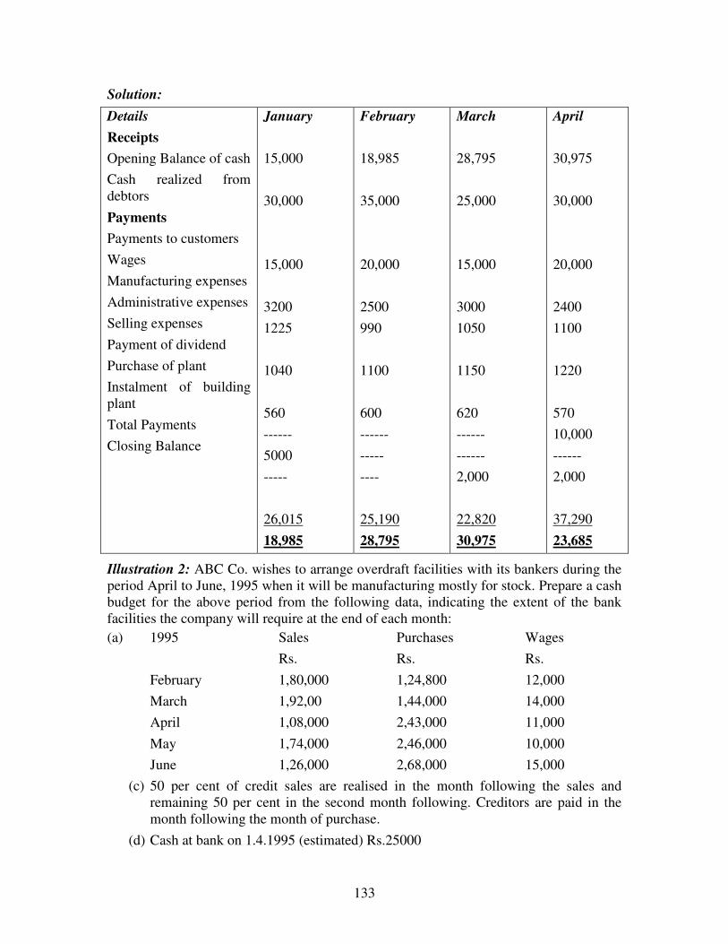
133
Solution:
Details
Receipts
Opening Balance of cash
Cash realized from
debtors
Payments
Payments to customers
Wages
Manufacturing expenses
Administrative expenses
Selling expenses
Payment of dividend
Purchase of plant
Instalment of building
plant
Total Payments
Closing Balance
January
15,000
30,000
15,000
3200
1225
1040
560
------
5000
-----
26,015
18,985
February
18,985
35,000
20,000
2500
990
1100
600
------
-----
----
25,190
28,795
March
28,795
25,000
15,000
3000
1050
1150
620
------
------
2,000
22,820
30,975
April
30,975
30,000
20,000
2400
1100
1220
570
10,000
------
2,000
37,290
23,685
Illustration 2: ABC Co. wishes to arrange overdraft facilities with its bankers during the
period April to June, 1995 when it will be manufacturing mostly for stock. Prepare a cash
budget for the above period from the following data, indicating the extent of the bank
facilities the company will require at the end of each month:
(a) 1995 Sales Purchases Wages
Rs. Rs. Rs.
February 1,80,000 1,24,800 12,000
March 1,92,00 1,44,000 14,000
April 1,08,000 2,43,000 11,000
May 1,74,000 2,46,000 10,000
June 1,26,000 2,68,000 15,000
(c) 50 per cent of credit sales are realised in the month following the sales and
remaining 50 per cent in the second month following. Creditors are paid in the
month following the month of purchase.
(d) Cash at bank on 1.4.1995 (estimated) Rs.25000

134
Solution:
Receipts
Opening Balance
Sales
Amount received from sales
Total Receipts
Payments
Purchase
Wages
Total Payments
Closing Balance (a-b)
April
25,000
90,000
96,000
2,11,000
1,44,000
14,000
1,58,000
53,000
May
53000
96,000
54,000
2,03,000
2,43,000
11,000
2,54,000
(-)51,000
June
(-) 51000
54000
87000
90000
246000
10000
256000
(-)1,66,000
Lets Sum Up
� Cash Management refers to management of ash and bank balance or in a broader
sense it is the management of cash inflows and outflows.
� Every firm must have minimum cash. There may be different motives for holding
cash. These may be Transactionary motive, Precautionary motive or Speculative
motive for holding cash.
� The objectives of cash management may be defined as meeting the cash outflows
and minimizing the cost of cash balance.
� Cash budget is the most important technique for planning the cash movement. It is
a summary of cash inflows and outflows during particular period. In cash budget
all expected receipts and payments are noted to find out the cash shortage or
surplus during that period.
� Optimum level of cash balance is the balance which firm should have in order to
minimize the cost of maintaining cash. Baumol’s model gives optimum cash
balance which aims at minimizing the total cost of maintaining cash. The Miller –
Orr model says that a firm should maintain its cash balance within a range of
lower and higher limit.
QUESTIONS
1 What are objectives of cash management?
2 Write short notes on:
(a) Lock box system
(b) Paying the Float
3 Explain the Baumol’s model of cash management?
4 Discuss the Miller – Orr model for determining the cash balance for the firm?
5 “Cash budget is an appropriate technique of cash management” Explain. What are
the different methods of preparing the cash budget?
134
5
RECEIVABLES MANAGEMENT
Smriti Chawla Shri Ram College of Commerce
University of Delhi Delhi
Introduction
A sound managerial control requires proper management of liquid assets and inventory.
These assets are a part of working capital of the business. An efficient use of financial resources
is necessary to avoid financial distress. Receivables result from credit sales. A concern is
required to allow credit sales in order to expand its sales volume. It is not always possible to sell
goods on cash basis only. Sometimes, other concerns in that line might have established a
practice of selling goods on credit basis. Under these circumstances, it is not possible to avoid
credit sales without adversely affecting sales. The increase in sales is also essential to increase
profitability. After a certain level of sales the increase in sales will not proportionately increase
production costs. The increase in sales will bring in more profits.
Thus, receivables constitute a significant portion of current assets of a firm. But, for
investment in receivables, a firm has to incur certain costs. Further, there is a risk of bad debts
also. It is, therefore, very necessary to have a proper control and management of receivables.
Meaning of Receivables
Receivables represent amounts owed to the firm as a result of sale of goods or services in
the ordinary course of business. These are claims of the firm against its customers and form part
of its current assets. Receivables are also known as accounts receivables, trade receivables,
customer receivables or book debts. The receivables are carried for the customers. The period of
credit and extent of receivables depends upon the credit policy followed by the firm. The purpose
CHAPTER OBJECTIVES
� Introduction � Meaning of Receivables � Costs of Maintaining Receivables � Factors influencing the size of receivables � Meaning and Objectives of Receivable Management � Dimensions of Receivable Management � Illustrations � Lets Sum Up � Questions
135
of maintaining or investing in receivables is to meet competition, and to increase the sales and
profits.
Costs of Maintaining Receivables
The allowing of credit to customers means giving funds for the customer’s use. The
concern incurs the following cost on maintaining receivables:
(1) Cost of Financing Receivables: When goods and services are provided on credit then
concern’s capital is allowed to be used by the customers. The receivables are financed from the
funds supplied by shareholders for long term financing and through retained earnings. The
concern incurs some cost for colleting funds which finance receivables.
(2) Cost of Collection: A proper collection of receivables is essential for receivables
management. The customers who do not pay the money during a stipulated credit period are sent
reminders for early payments. Some persons may have to be sent for collection these amounts.
All these costs are known as collection costs which a concern is generally required to incur.
(3) Bad Debts : Some customers may fail to pay the amounts due towards them. The
amounts which the customers fail to pay are known as bad debts. Though a concern may be able
to reduced bad debts through efficient collection machinery but one cannot altogether rule out
this cost.
Factors Influencing the Size of Receivables
Besides sales, a number of other factors also influence the size of receivables. The
following factors directly and indirectly affect the size of receivables.
(1) Size of Credit Sales: The volume of credit sales is the first factor which increases or
decreases the size of receivables. If a concern sells only on cash basis as in the case of Bata Shoe
Company, then there will be no receivables. The higher the part of credit sales out of total sales,
figures of receivables will also be more or vice versa.
(2) Credit Policies: A firm with conservative credit policy will have a low size of
receivables while a firm with liberal credit policy will be increasing this figure. If collections are
prompt then even if credit is liberally extended the size of receivables will remain under control.
In case receivables remain outstanding for a longer period, there is always a possibility of bad
debts.
(3) Terms of Trade: The size of receivables also depends upon the terms of trade. The
period of credit allowed and rates of discount given are linked with receivables. If credit period
allowed is more then receivables will also be more. Sometimes trade policies of competitors
have to be followed otherwise it becomes difficult to expand the sales.
(4) Expansion Plans: When a concern wants to expand its activities, it will have to enter
new markets. To attract customers, it will give incentives in the form of credit facilities. The
period of credit can be reduced when the firm is able to get permanent customers. In the early
stages of expansion more credit becomes essential and size of receivables will be more.
(5) Relation with Profits: The credit policy is followed with a view to increase sales.
When sales increase beyond a certain level the additional costs incurred are less than the increase
in revenues. It will be beneficial to increase sales beyond the point because it will bring more

136
profits. The increase in profits will be followed by an increase in the size of receivables or vice-
versa.
(6) Credit Collection Efforts: The collection of credit should be streamlined. The
customers should be sent periodical reminders if they fail to pay in time. On the other hand, if
adequate attention is not paid towards credit collection then the concern can land itself in a
serious financial problem. An efficient credit collection machinery will reduce the size of
receivables.
(7) Habits of Customers: The paying habits of customers also have bearing on the size of
receivables. The customers may be in the habit of delaying payments even though they are
financially sound. The concern should remain in touch with such customers and should make
them realise the urgency of their needs.
Meaning and Objectives of Receivables Management
Receivables management is the process of making decisions relating to investment in
trade debtors. We have already stated that certain investment in receivables is necessary to
increase the sales and the profits of a firm. But at the same time investment in this asset involves
cost considerations also. Further, there is always a risk of bad debts too. Thus, the objective of
receivables management is to take a sound decision as regards investment in debtors. In the
words of Bolton, S.E., the objectives of receivables management is “to promote sales and profits
until that point is reached where the return on investment in further funding of receivables is less
than the cost of funds raised to finance that additional credit.”
Dimensions of Receivables Management
Receivables management involves the careful consideration of the following aspects:
1. Forming of credit policy.
2. Executing the credit policy.
3. Formulating and executing collection policy.
1. Forming of Credit Policy
For efficient management of receivables, a concern must adopt a credit policy. A credit
policy is related to decisions such as credit standards, length of credit period, cash discount and
discount period, etc.
(a) Quality of Trade Accounts of Credit Standards: The volume of sales will be
influenced by the credit policy of a concern. By liberalising credit policy the volume of sales can
be increased resulting into increased profits. The increased volume of sales is associated with
certain risks too. It will result in enhanced costs and risks of bad debts and delayed receipts. The
increase in number of customers will increase the clerical wok of maintaining the additional
accounts and collecting of information about the credit worthiness of customers. There may be
more bad debt losses due to extension of credit to less worthy customers. These customers may
also take more time than normally allowed in making the payments resulting into tying up of
additional capital in receivables. On the other hand, extending credit to only credit worthy
customers will save costs like bad debt losses, collection costs, investigation costs, etc. The
restriction of credit to such customers only will certainly reduce sales volume, thus resulting in
reduced profits.

137
A finance manager has to match the increased revenue with additional costs. The credit
should be liberalised only to the level where incremental revenue matches the additional costs.
The quality of trade accounts should be decided so that credit facilities are extended only upto
that level. The optimum level of investment in receivables should be where there is a trade off
between the costs and profitability. On the other hand, a tight credit policy increases the liquidity
of the firm. On the other hand, a tight credit policy increases the liquidity of the firm. Thus,
optimum level of investment in receivables is achieved at a point where there is a trade off
between cost, profitability and liquidity as depicted below:
(b) Length of Credit Period: Credit terms or length of credit period means the period
allowed to the customers for making the payment. The customers paying well in time may also
be allowed certain cash discount. A concern fixes its own terms of credit depending upon its
customers and the volume of sales. The competitive pressure from other firms compels to follow
similar credit terms, otherwise customers may feel inclined to purchase from a firm which allows
more days for paying credit purchases. Sometimes more credit time is allowed to increase sales
to existing customers and also to attract new customers. The length of credit period and quantum
of discount allowed determine the magnitude of investment in receivables.
(c) Cash Discount: Cash discount is allowed to expedite the collection of receivables.
The concern will be able to use the additional funds received from expedited collections due to
cash discount. The discount allowed involves cost. The discount should be allowed only if its
cost is less than the earnings from additional funds. If the funds cannot be profitably employed
then discount should not be allowed.
(d) Discount Period: The collection of receivables is influenced by the period allowed
for availing the discount. The additional period allowed for this facility may prompt some more
customers to avail discount and make payments. This will mean additional funds released from
receivables which may be alternatively used. At the same time the extending of discount period
will result in late collection of funds because those who were getting discount and making
payments as per earlier schedule will also delay their payments.

138
2. Executing Credit Policy
After formulating the credit policy, its proper execution is very important. The evaluation
of credit applications and finding out the credit worthiness of customers should be undertaken.
(a) Collecting Credit information: The first step in implementing credit policy will be to
gather credit information about the customers. This information should be adequate enough so
that proper analysis about the financial position of the customers is possible. This type of
investigation can be undertaken only upto a certain limit because it will involve cost.
The sources from which credit information will be available should be ascertained. The
information may be available from financial statements, credit rating agencies, reports from
banks, firm’s records etc. Financial reports of the customer for a number of years will be helpful
in determining the financial position and profitability position. The balance sheet will help in
finding out the short term and long term position of the concern. The income statements will
show the profitability position of concern. The liquidity position and current assets movement
will help in finding out the current financial position. A proper analysis of financial statements
will be helpful in determining the credit worthiness of customers. There are credit rating
agencies which can supply information about various concerns. These agencies regularly collect
information about business units from various sources and keep this information upto date. The
information is kept in confidence and may be used when required.
Credit information may be available with banks too. The banks have their credit
departments to analyse the financial position of a customer.
In case of old customers, business own records may help to know their credit worthiness.
The frequency of payments, cash discounts availed, interest paid on over due payments etc. may
help to form an opinion about the quality of credit.
(b) Credit Analysis: After gathering the required information, the finance manager should
analyse it to find out the credit worthiness of potential customers and also to see whether they
satisfy the standards of the concern or not. The credit analysis will determine the degree of risk
associated with the account, the capacity of the customer borrow and his ability and willingness
to pay.
(c) Credit Decision: After analysing the credit worthiness of the customer, the finance
manager has to take a decision whether the credit is to be extended and if yes then upto what
level. He will match the creditworthiness of the customer with the credit standards of the
company. If customer’s creditworthiness is above the credit standards then there is no problem in
taking a decision. It is only in the marginal case that such decisions are difficult to be made. In
such cases the benefit of extending the credit should be compared to the likely bad debt losses
and then decision should be taken. In case the customers are below the company credit standards
then they should not be outrightly refused. Rather they should be offered some alternative
facilities. A customer may be offered to pay on delivery of goods, invoices may be sent through
bank. Such a course help in retaining the customers at present and their dealings may help in
reviewing their requests at a later date.
(d) Financing Investments in Receivables and Factoring: Accounts receivables block a
part of working capital. Efforts should be made that funds are not tied up in receivables for
longer periods. The finance manager should make efforts to get receivables financed so that
working capital needs are met in time. The quality of receivables will determine the amount of
139
loan. The banks will accept receivable of dependable parties only. Another method of getting
funds against receivables is their outright sale to the bank. The bank will credit the amount to the
party after deducting discount and will collect the money from the customers later. Here too, the
bank will insist on quality receivables only. Besides banks, there may be other agencies which
can buy receivables and pay cash for them. This facility is known as factoring. The factoring
may be with or without recourse. It is without recourse then any bad debt loss is taken up by the
factor but if it is with recourse then bad debts losses will be recovered from the seller.
Factoring is collection and finance service designed to improve he cash flow position of the
sellers by converting sales invoices into ready cash. The procedure of factoring can be explained
as follows:
1. Under an agreement between the selling firm and factor firm, the latter makes an
appraisal of the credit worthiness of potential customers and may also set the credit limit
and term of credit for different customers.
2. The sales documents will contain the instructions to make payment directly to factor who
is responsible for collection.
3. When the payment is received by the factor on the due date the factor shall deduct its
fees, charges etc and credit the balance to the firm’s accounts.
4. In some cases, if agreed the factor firm may also provide advance finance to selling firm
for which it may charge from selling firm. In a way this tantamount to bill discounting by
the factor firm. However factoring is something more than mere bill discounting, as the
former includes analysis of the credit worthiness of the customer also. The factor may
pay whole or a substantial portion of sales vale to the selling firm immediately on sales
being effected. The balance if any, may be paid on normal due date.
Benefits and Cost of Factoring
A firm availing factoring services may have the following benefits:
� Better Cash Flows
� Better Assets Management
� Better Working Capital Management
� Better Administration
� Better Evaluation
� Better Risk Management
However, the factoring involves some monetary and non-monetary costs as follows:
Monetary Costs
a) The factor firm charges substantial fees and commission for collection of receivables.
These charges sometimes may be too much in view of amount involved.
b) The advance fiancé provided by factor firm would be available at a higher interest
costs than usual rate of interest.

140
Non-Monetary Costs
a) The factor firm doing the evaluation of credit worthiness of the customer will be
primarily concerned with the minimization of risk of delays and defaults. In the process it
may over look sales growth aspect.
b) A factor is in fact a third party to the customer who may not feel comfortable while
dealing with it.
c) The factoring of receivables may be considered as a symptom of financial weakness.
Factoring in India is of recent origin. In order to study the feasibility of factoring services in
India, the Reserve Bank of India constituted a study group for examining the introduction of
factoring services, which submitted its report in 1988.On the basis of the recommendations of
this study group the RBI has come out with specific guidelines permitting a banks to start
factoring in India through their subsidiaries. For this country has been divided into four zones. In
India the factoring is still not very common. The first factor i.e. The SBI Factor and Commercial
Services Limited started working in April 1991. The guidelines for regulation of a factoring are
as follows:
(1) A factor firm requires an approval from Reserve Bank of India.
(2) A factor firm may undertake factoring business or other incidental activities.
(3) A factor firm shall not engage in financing of other firms or firms engaged in
factoring.
3. Formulating and Executing Collection Policy
The collection o f amounts due to the customers is very important. The collection policy
the termed as strict and lenient. A strict policy of collection will involve more efforts on
collection. Such a policy has both positive and negative effects. This policy will enable early
collection of dues and will reduce bad debt losses. The money collected will be used for other
purposes and the profits of the concern will go up. On the other hand a rigorous collection policy
will involve increased collection costs. It may also reduce the volume of sales. A lenient policy
may increase the debt collection period and more bad debt losses. A customer not clearing the
dues for long may not repeat his order because he will have to pay earlier dues first, thus causing.
The objective is to collect the dues and not to annoy the customer. The steps should be
like (i) sending a reminder for payments (ii) Personal request through telephone etc. (iii)
Personal visits to the customers (iv) Taking help of collecting agencies and lastly (v) Taking
legal action. The last step should be taken only after exhausting all other means because it will
have a bad impact on relations with customers.
Illustration 1: A company has prepared the following projections for a year
Sales 21000 units
Selling Price per unit Rs.40
Variable Costs per unit Rs.25
Total Costs per unit Rs.35
Credit period allowed One month

141
The company proposes to increase the credit period allowed to its customers from one month to
two months .It is envisaged that the change in policy as above will increase the sales by 8%. The
company desires a return of 25% on its investment. You are required to examine and advise
whether the proposed credit policy should be implemented or not?
Solution:
Particulars Present Proposed Incremental
Sales (units)
Contribution per unit
Total Contribution
Variable cost @ Rs.25
Fixed Cost
Total Cost
Credit period
Average debtors at cost
21000
Rs.15
Rs.3,15,000
5,25,000
2,10,000
7,35,000
1 month
Rs.61250
22680
Rs.15
Rs.3,40,000
5,67,000
2,10,000
7,77,000
2 month
Rs.1,29,500
1680
Rs.15
Rs.25,200
42,000
------
42,000
-----
Rs.68,250
Incremental Return = Increased Contribution/Extra Funds
Blockage *100
= Rs.25,200/Rs.68,250*100
=36.92%
Illustration 2: ABC & Company is making sales of Rs.16,00,000 and it extends a credit of 90
days to its customers. However, in order to overcome the financial difficulties, it is considering
to change the credit policy. The proposed terms of credit and expected sales are given hereunder:
Policy Terms Sales
I 75 days Rs.15,00,000
II 60 days Rs. 14,50,000
III 45 days Rs 14,25,000
IV 30 days Rs 13,50,000
V 15 days Rs.13,00,000
The firm has variable cost of 80% and fixed cost of Rs.1,00,000. The cost of capital is 15%.
Evaluate different policies and which policy should be adopted?

142
Solution:
figures in Rs.
Particulars Present I II III IV V
Sales
-- Variable
cost
-- Fixed
Cost
Profit (A)
Total Cost
Average
Receivable
(at cost)
(Cost÷360x
credit
period
Cost of
debtors @
15% (B)
Net profit
(A – B)
16,00,000
12,80,000
1,00,000
2,20,000
13,80,000
3,45,000
51,750
1,68,250
15,00,000
12,00,000
1,00,000
2,00,000
13,00,000
2,70,833
40,625
1,59,350
14,50,000
11,60,000
1,00,000
1,90,000
12,60,000
2,10,000
31,500
1,58,500
14,25,000
11,40,000
1,00,000
1,85,000
12,40,000
1,55,000
23,250
1,61,750
13,50,000
10,80,000
1,00,000
1,70,000
11,80,000
98,333
14,750
1,55,250
13,00,000
10,40,000
1,00,000
1,60,000
11,40,000
47,500
7,125
1,52,875
Illustration3: A trader whose current sales are Rs.15 lakhs per annum and average collection
period is 30 days wants to pursue a more liberal credit policy to improve sales. A study made by
consultant firm reveals the following information.
Credit Policy increase in collection period Increase in sales
A 15 days Rs.60,000
B 30 days 90,000
C 45 days 1,50,000
D 60 days 1,80,000
E 90 days 2,00,000

143
The selling price per unit is Rs.5. Average Cost per unit is Rs.4 and variable cost per unit I
Rs.2.75 paise per unit. The required rate of return on additional investments is 20 percent
Assume 360 days a year and also assume that there are no bad debts. Which of the above policies
would you recommend for adoption.
Solution:
Particulars Present A B C D E
Credit period
No. of units
@ Rs.5
Sales
Variable
cost@ 2.75
Fixed Cost
Total Cost
Profit (A)
Average
debtors(at
cost)
cost÷360x
credit period
Cost of
investment@
20% (B)
Net Profit
(A-B)
30 days
3,00,000
15,00,000
8,25,000
3,75,000
12,00,000
3,00,000
1,00,000
20,000
2,80,000
45 days
3,12,000
15,60,000
8,58,000
3,75,000
12,33,000
3,27,000
1,54,125
30,825
2,96,175
60 days
3,18,000
15,90,000
8,74,500
3,75,000
12,49,500
3,40,500
2,08,250
41,650
2,98,850
75 days
3,30,000
16,50,000
9,07,500
3,75,000
12,82,500
3,67,500
2,67,188
53,437
3,14,063
90 days
3,36,000
16,80,000
9,24,000
3,75,000
12,99,000
3,81,000
3,24,750
64,950
3,16,050
120 days
3,40,000
17,00,000
9,35,000
3,75,000
13,10,000
3,90,000
4,36,667
87,333
3,02,667

144
Lets Sum Up
� The receivables emerge when goods are sold on credit and the payments are deferred by
the customers. So, every firm should have a well-defined credit policy.
� The receivables management refers to managing the receivables in the light of costs and
benefit associated with a particular credit policy.
� Receivables management involves the careful consideration of the following aspects:
Forming of credit policy, Executing the credit policy, Formulating and executing
collection policy.
� The credit policy deals with the setting of credit standards and credit terms relating to
discount and credit period.
� The credit evaluation includes the steps required for collection and analysis of
information regarding the credit worthiness of the customer.
QUESTIONS
1. What do you understand by Receivables Management? Discuss the factors which influence
the size of receivables?
2. What should be the considerations in forming a credit policy?
3. “Receivables forecasting is important for the proper management of receivables
forecasting.” Explain.
4. Discuss the various aspects or dimensions of receivable management?
5. Write short note on Factoring.

145
6
INVENTORY MANAGEMENT
Smriti Chawla Shri Ram College of Commerce
University of Delhi Delhi
Introduction
Every enterprise needs inventory for smooth running of its activities. It serves as a link
between production and distribution processes. There is, generally, a time lag between the
recognition of need and its fulfilment. The greater the time – lag, the higher the requirements for
inventory.
The investment in inventories constitutes the most significant part of current
assets/working capital in most of the undertakings. Thus, it is very essential to have proper
control and management of inventories. The purpose of inventory management is to ensure
availability of materials in sufficient quantity as and when required and also to minimise
investment in inventories.
Meaning and Nature of inventory
In accounting language it may mean stock of finished goods only. In a manufacturing
concern, it may include raw materials, work in process and stores, etc. Inventory includes the
following things:
(a) Raw Material: Raw material form a major input into the organisation. They are
required to carry out production activities uninterruptedly. The quantity of raw materials required
will be determined by the rate of consumption and the time required for replenishing the
CHAPTER OBJECTIVES � Introduction � Meaning and nature of inventory � Purpose/Benefits of Holding Inventory � Risks/Costs of Holding inventory � Inventory Management � Objects of Inventory Management � Tools and Techniques of Inventory Management � Risks in Inventory Management � Lets Sum Up � Questions

146
supplies. The factors like the availability of raw materials and government regulations etc. too
affect the stock of raw materials.
(b) Work in Progress: The work-in-progress is that stage of stocks which are in between
raw materials and finished goods. The raw materials enter the process of manufacture but they
are yet to attain a final shape of finished goods. The quantum of work in progress depends upon
the time taken in the manufacturing process. The greater the time taken in manufacturing, the
more will be the amount of work in progress.
(c) Consumables: These are the materials which are needed to smoothen the process of
production. These materials do not directly enter production but they act as catalysts, etc.
Consumables may be classified according to their consumption and criticality.
(d) Finished goods: These are the goods which are ready for the consumers. The stock of
finished goods provides a buffer between production and market. The purpose of maintaining
inventory is to ensure proper supply of goods to customers.
(e) Spares: Spares also form a part of inventory. The consumption pattern of raw
materials, consumables, finished goods are different from that of spares. The stocking policies of
spares are different from industry to industry. Some industries like transport will require more
spares than the other concerns. The costly spare parts like engines, maintenance spares etc. are
not discarded after use, rather they are kept in ready position for further use.
Purpose/Benefits of Holding Inventors
There are three main purposes or motives of holding inventories:
(i) The Transaction Motive which facilitates continuous production and timely execution
of sales orders.
(ii) The Precautionary Motive which necessitates the holding of inventories for meeting
the unpredictable changes in demand and supplies of materials.
(iii) The Speculative Motive which induces to keep inventories for taking advantage of
price fluctuations, saving in re-ordering costs and quantity discounts, etc.
Risk and Costs of Holding Inventors
The holding of inventories involves blocking of a firm’s funds and incurrence of capital and
other costs. It also exposes the firm to certain risks. The various costs and risks involved in
holding inventories are as below:
(i) Capital costs: Maintaining of inventories results in blocking of the firm’s financial
resources. The firm has, therefore, to arrange for additional funds to meet the cost of
inventories. The funds may be arranged from own resources or from outsiders. But in
both cases, the firm incurs a cost. In the former case, there is an opportunity cost of
investment while in later case the firm has to pay interest to outsiders.
(ii) Cost of Ordering: The costs of ordering include the cost of acquisition of inventories.
It is the cost of preparation and execution of an order, including cost of paper work
and communicating with supplier. There is always minimum cot involve whenever an
order for replenishment of good is placed. The total annual cost of ordering is equal to
cost per order multiplied by the number of order placed in a year.

147
(iii) Cost of Stock-outs: A stock out is a situation when the firm is not having units of an
item in store but there is demand for that either from the customers or the production
department. The stock out refer to demand for an item whose inventory level is
reduced to zero and insufficient level. There is always a cost of stock out in the sense
that the firm faces a situation of lost sales or back orders. Stock out are quite often
expensive.
(iv) Storage and Handling Costs. Holding of inventories also involves costs on storage as
well as handling of materials. The storage costs include the rental of the godown,
insurance charge etc.
(v) Risk of Price Decline. There is always a risk of reduction in the prices of inventories
by the suppliers in holding inventories. This may be due to increased market supplies,
competition or general depression in the market.
(vi) Risk of Obsolescence. The inventories may become obsolete due to improved
technology, changes in requirements, change in customer’s tastes etc.
(vii) Risk Deterioration in Quality: The quality of the materials may also deteriorate
while the inventories are kept in stores.
Inventory Management
It is necessary for every management to give proper attention to inventory management.
A proper planning of purchasing, handling storing and accounting should form a part of
inventory management. An efficient system of inventory management will determine (a) what to
purchase (b) how much to purchase (c) from where to purchase (d) where to store, etc.
There are conflicting interests of different departmental heads over the issue of inventory.
The finance manager will try to invest less in inventory because for him it is an idle investment,
whereas production manager will emphasise to acquire more and more inventory as he does not
want any interruption in production due to shortage of inventory. The purpose of inventory
management is to keep the stocks in such a way that neither there is over-stocking nor under-
stocking. The over-stocking will mean reduction of liquidity and starving of other production
processes; under-stocking, on the other hand, will result in stoppage of work. The investments in
inventory should be kept in reasonable limits.
Objects of Inventory Management
The main objectives of inventory management are operational and financial. The operational
objectives mean that the materials and spares should be available in sufficient quantity so that
work is not disrupted for want of inventory. The financial objective means that investments in
inventories should not remain idle and minimum working capital should be locked in it. The
following are the objectives of inventory management:
(1) To ensure continuous supply of materials spares and finished goods so that production
should not suffer at any time and the customers demand should also be met.
(2) To avoid both over-stocking and under-stocking of inventory.
(3) To keep material cost under control so that they contribute in reducing cost of production
and overall costs.
(4) To minimise losses through deterioration, pilferage, wastages and damages.

148
(5) To ensure perpetual inventory control so that materials shown in stock ledgers should be
actually lying in the stores.
(6) To ensure right quality goods at reasonable prices.
(7) To maintain investments in inventories at the optimum level as required by the
operational and sales activities.
(8) To eliminate duplication in ordering or replenishing stocks. This is possible with help of
centralising purchases.
(9) To facilitate furnishing of data for short term and long term planning and control of
inventory.
(10) To design proper organisation of inventory. A clear cut accountability should be fixed at
various levels of management.
Tools and Techniques of inventory Management
Effective Inventory management requires an effective control system for inventories. A
proper inventory control not only helps in solving the acute problem of liquidity but also
increases profits and causes substantial reduction in the working capital of the concern. The
following are the important tools and techniques of inventory management and control:
1. Determination of Stock Levels.
2. Determination of Safety Stocks.
3. Determination of Economic Order Quantity
4. A.B.C. Analysis
5. VED Analysis
6. Inventory Turnover Ratios
7. Aging Schedule of Inventories
8. Just in Time Inventory
1. Determination of Stock Levels
Carrying of too much and too little of inventories is detrimental to the firm. If the
inventory level is too little, the firm will face frequent stock-outs involving heavy ordering cost
and if the inventory level is too high it will be unnecessary tie-up of capital. Therefore, an
efficient inventory management requires that a firm should maintain an optimum level of
inventory where inventory costs are the minimum and at the same time there is not stock-out
which may result in loss of sale or stoppage of production. Various stock levels are discussed as
such.
(a) Minimum Level: This represents the quantity which must be maintained in hand at all times.
If stocks are less than the minimum level then the work will stop due to shortage of
materials. Following factors are taken into account while fixing minimum stock level:
Lead Time: A purchasing firm requires some time to process the order and time is also
required by supplying firm to execute the order. The time taken in processing the order and then
executing it is known as lead time.

149
Rate of Consumption: It is the average consumption of materials in the factory. The rate of
consumption will be decided on the basis pas experiences and production plans.
Nature of Material: The nature of material also affects the minimum level. If material is required
only against special orders of customer then minimum stock will not be required for such
materials.
Minimum stock level = Re-ordering level-(Normal consumption
x Normal Re-order period).
(b) Re-ordering Level: When the quantity of materials reaches at a certain figure then fresh
order is sent to get materials again. The order is sent before the materials reach minimum stock
level. Reordering level is fixed between minimum and maximum level. The rate of consumption,
number of days required to replenish the stock and maximum quantity of material required on
any day are taken into account while fixing reordering level.
Re-ordering Level = Maximum Consumption x Maximum Re-order period.
(c) Maximum Level: It is the quantity of materials beyond which a firm should not exceed its
stocks. If the quantity exceeds maximum level limit then it will be overstocking. A firm should
avoid overstocking because it will result in high material costs.
Maximum Stock Level = Re-ordering Level+ Re-ordering Quantity
-(Minimum Consumption x Minimum Re-ordering period).
(d) Danger Level: It is the level beyond which materials should not fall in any case. If danger
level arises then immediate steps should be taken to replenish the stock even if more cost is
incurred in arranging the materials. If materials are not arranged immediately there is possibility
of stoppage of work.
Danger Level = Average Consumption x Maximum reorder period
for emergency purchases.
(e) Average Stock Level
The average stock level is calculated as such:
Average Stock level = Minimum Stock Level +½ of re-order quantity
2. Determination of Safety Stocks
Safety stock is a buffer to meet some unanticipated increase in usage. It fluctuates over a
period of time. The demand for materials may fluctuate and delivery of inventory may also be
delayed and in such a situation the firm can face a problem of stock-out. The stock-out can prove
costly by affecting the smooth working of the concern. In order to protect against the stock out
arising out of usage fluctuations, firms usually maintain some margin of safety or safety stocks.
Two costs are involved in the determination of this stock i.e. opportunity cost of stock-outs and
the carrying costs. The stock out of raw materials cause production disruption resulting in higher
cost of production. Similarly, the stock out of finished goods result into failure of firm in
competition, as firm cannot provide proper customer service. If a firm maintains low level of
safety frequent stock out will occur resulting in large opportunity coast. On the other hand larger
quantity of safety stock involves higher carrying costs.

150
3. Economic Order Quantity (EOQ)
A decision about how much to order has great significance in inventory management.
The quantity to be purchased should neither be small nor big because costs of buying and
carrying materials are very high. Economic order quantity is the size of the lot to be purchased
which is economically viable. This is the quantity of materials which can be purchased at
minimum costs. Generally, economic order quantity is the point at which inventory carrying
costs are equal to order costs. In determining economic order quantity it is assumed that cost of a
managing inventory is made of solely of two parts i.e. ordering costs and carrying costs.
(A) Ordering Costs: These are costs that are associated with the purchasing or ordering of
materials. These costs include:
(1) Inspection costs of incoming materials.
(2) Cost of stationery, typing, postage, telephone charges etc.
(3) Expenses incurred on transportation of goods purchased.
These costs are also know as buying costs and will arise only when some purchases are made.
(B) Carrying Costs: These are costs for holding the inventories. These costs will not be
incurred if inventories are not carried. These costs include:
(1) The cost of capital invested in inventories. An interest will be paid on the amount of
capital locked up in inventories.
(2) Cost of storage which could have been used for other purposes.
(3) Insurance Cost
(4) Cost of spoilage in handling of materials
Assumptions of EOQ: While calculating EOQ the following assumptions are made.
1. The supply of goods is satisfactory. The goods can be purchased whenever these are
needed.
2. The quality to be purchased by the concern is certain.
3. The prices of goods are stable. It results to stabilise carrying costs.
Economic order quantity can be calculated with the help of the following formula:
I
ASEOQ
2=
where, A = Annual consumption in rupees.
S = Cost of placing an order.
I = Inventory carrying costs of one unit.
Illustration 1: The finance department of a Corporation provides the following information:
(i) The carrying costs per unit of inventory are Rs. 10
(ii) The fixed costs per order are Rs. 20]
(iii) The number of units required is 30,000 per year.

151
Determine the economic order quantity (EOQ) total number of orders in a year and the time
gap between orders.
Solution: The economic order quantity may be found as follow
I
ASEOQ
2=
A = 30,000
S = Rs.20
I = Rs.10
Now, EOQ = ( 2 x 30,000x 20) ÷ 10 )1/2
= 346 units
So, the EOQ is 346 units and the number of orders in a year would be 30,000/346 = 86.7 or 87
orders. The time gap between two orders would be 365/87 = 4.2 or 4 days.
4. A-B-C Analysis
Under A-B-C analysis, the materials are divided into three categories viz, A, B and C.
Past experience has shown that almost 10 per cent of the items contribute to 70 percent of value
of consumption and this category is called ‘A’ Category. About 20 per cent of value of
consumption and this category is called ‘A’ Category. About 20 per cent of the items contribute
about 20 per cent of value of consumption and this is known as category ‘B’ materials. Category
‘C’ covers about 70 per cent of items of materials which contribute only 10 per cent of value of
consumption. There may be some variation in different organisations and an adjustment can be
made in these percentages.
The information is shown in the following diagram:
Class No. of Items (%) Value of Items (%)
A 10 70
B 20 20
C 70 10

152
A-B-C analysis helps to concentrate more efforts on category A since greatest monetary
advantage will come by controlling these items. An attention should be paid in estimating
requirements, purchasing, maintaining safety stocks and properly storing of ‘A’ category
materials. These items are kept under a constant review so that substantial material cost may be
controlled. The control of ‘C’ items may be relaxed and these stocks may be purchased for the
year. A little more attention should be given towards ‘B’ category items and their purchase
should be undertaken a quarterly or half-yearly intervals.
5. VED Analysis
The VED analysis is used generally for spare parts. The requirements and urgency of
spare parts is different from that of materials. A-B-C analysis may not be properly used for spare
parts. Spare parts are classified as Vital (V), Essential (E) and Desirable (D) The vital spares are
a must for running the concern smoothly and these must be stored adequately. The non-
availability of vital spares will cause havoc in the concern. The E type of spares are also
necessary but their stocks may be kept at low figures. The stocking of D type of spares may be
avoided at times. If the lead time of these spares is less, then stocking of these spares can be
avoided.
6. Inventory Turnover Ratios
Inventory turnover ratios are calculated to indicate whether inventories have been used
efficiently or not. The purpose is to ensure the blocking of only required minimum funds in
inventory. The Inventory Turnover Ratio also known as stock velocity is normally calculated as
sales/average inventory or cost of goods sold/average inventory cost.
Inventory Turnover Ratio = CostatInventoryAverage
SoldGoodsofCost
InventoryAverage
SalesNet
)(=
and, Inventory Conversion Period = RatioTurnoverInventory
yearainDays
7. Aging Schedule of Inventories
Classification of inventories according to the period (age) of their holding also helps in
identifying slow moving inventories thereby helping in effective control and management of
inventories. The following table show aging of inventories of a firm.
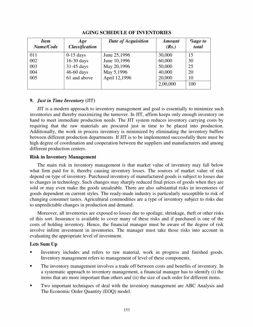
153
AGING SCHEDULE OF INVENTORIES
Item
Name/Code
Age
Classification
Date of Acquisition Amount
(Rs.)
%age to
total
011
002
003
004
005
0-15 days
16-30 days
31-45 days
46-60 days
61 and above
June 25,1996
June 10,1996
May 20,1996
May 5,1996
April 12,1996
30,000
60,000
50,000
40,000
20,000
15
30
25
20
10
2,00,000 100
9. Just in Time Inventory (JIT)
JIT is a modern approach to inventory management and goal is essentially to minimize such
inventories and thereby maximizing the turnover. In JIT, affirm keeps only enough inventory on
hand to meet immediate production needs. The JIT system reduces inventory carrying costs by
requiring that the raw materials are procured just in time to be placed into production.
Additionally, the work in process inventory is minimized by eliminating the inventory buffers
between different production departments. If JIT is to be implemented successfully there must be
high degree of coordination and cooperation between the suppliers and manufacturers and among
different production centers.
Risk in Inventory Management
The main risk in inventory management is that market value of inventory may fall below
what firm paid for it, thereby causing inventory losses. The sources of market value of risk
depend on type of inventory. Purchased inventory of manufactured goods is subject to losses due
to changes in technology. Such changes may sharply reduced final prices of goods when they are
sold or may even make the goods unsaleable. There are also substantial risks in inventories of
goods dependent on current styles. The ready-made industry is particularly susceptible to risk of
changing consumer tastes. Agricultural commodities are a type of inventory subject to risks due
to unpredictable changes in production and demand.
Moreover, all inventories are exposed to losses due to spoilage, shrinkage, theft or other risks
of this sort. Insurance is available to cover many of these risks and if purchased is one of the
costs of holding inventory. Hence, the financial manager must be aware of the degree of risk
involve infirm investment in inventories. The manager must take those risks into account in
evaluating the appropriate level of investment.
Lets Sum Up
� Inventory includes and refers to raw material, work in progress and finished goods.
Inventory management refers to management of level of these components.
� The inventory management involves a trade off between costs and benefits of inventory. In
a systematic approach to inventory management, a financial manager has to identify (i) the
items that are more important than others and (ii) the size of each order for different items.
� Two important techniques of deal with the inventory management are ABC Analysis and
The Economic Order Quantity (EOQ) model.

154
� The EOQ model attempts to find out the number of units to be ordered every time in order
to minimize the total cost of ordering and carrying the inventory.
QUESTIONS
1 Write short notes on:
(a) ABC Analysis of inventory control
(b) Economic order quantity
2 Define safety stock. How is it determined? What is the role of safety stock in
inventory management?
3. What is the need for holding inventory? Why inventory management is important?
4. Explain briefly techniques of inventory management.