graduate macro theory ii: notes on using dynareesims1/using_dynare_sp15.pdf · graduate macro...

Graduate Macro Theory II:

Notes on Using Dynare

Eric Sims

University of Notre Dame

Spring 2015

1 Introduction

This document will present some simple examples of how to solve and simulate DSGE models

using Dynare. Dynare can also be used to estimate the parameters of DSGE models via Maximum

Likelihood or Bayesian Maximum Likelihood.

Dynare is not its own program but is rather basically a collection of Matlab codes. To run

Dynare, you must first install it. You can download it from the following website: http://www.

dynare.org/download. I will only support downloads using Matlab. You need to choose a

destination folder. My destination folder is in the C drive and is called “dynare”. I have version

4.4.3, the newest “stable” version (older versions will do most of the basic stuff just as well as the

current version).. The full path is: “C:\dynare \4.4.3 \matlab ”.

To run Dynare, you have to create .mod files (you can create these in the m-file editor, but be

sure to save them as .mod, not as .m files). Then, to run your code, simply type “dynare filename”

into the command window (or you can have this command within a seperate m-file which can be

in another directory so long as you call up the Dynare directory). Equivalently, you can “set the

path” in Matlab so that you don’t always have to call up the Dynare directory.

2 A Neoclassical Model with Fixed Labor

Consider a simple stochastic neoclassical model with fixed labor as the laboratory. The planner’s

problem can be written:

max E0

∞∑t=0

βtc1−σt − 1

1− σ

s.t.

kt+1 = atkαt − ct + (1− δ)kt

1

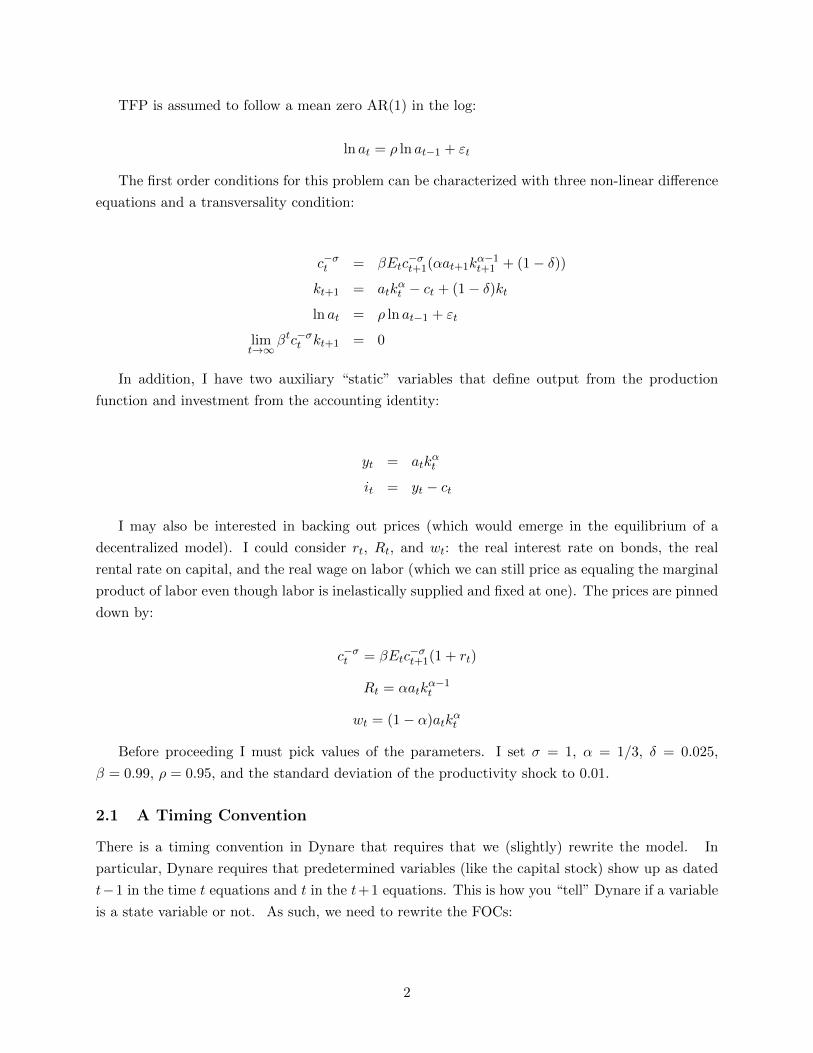
TFP is assumed to follow a mean zero AR(1) in the log:

ln at = ρ ln at−1 + εt

The first order conditions for this problem can be characterized with three non-linear difference

equations and a transversality condition:

c−σt = βEtc−σt+1(αat+1k

α−1t+1 + (1− δ))

kt+1 = atkαt − ct + (1− δ)kt


limt→∞

βtc−σt kt+1 = 0

In addition, I have two auxiliary “static” variables that define output from the production

function and investment from the accounting identity:

yt = atkαt

it = yt − ct

I may also be interested in backing out prices (which would emerge in the equilibrium of a

decentralized model). I could consider rt, Rt, and wt: the real interest rate on bonds, the real

rental rate on capital, and the real wage on labor (which we can still price as equaling the marginal

product of labor even though labor is inelastically supplied and fixed at one). The prices are pinned

down by:

c−σt = βEtc−σt+1(1 + rt)

Rt = αatkα−1t

wt = (1− α)atkαt

Before proceeding I must pick values of the parameters. I set σ = 1, α = 1/3, δ = 0.025,

β = 0.99, ρ = 0.95, and the standard deviation of the productivity shock to 0.01.

2.1 A Timing Convention

There is a timing convention in Dynare that requires that we (slightly) rewrite the model. In

particular, Dynare requires that predetermined variables (like the capital stock) show up as dated

t−1 in the time t equations and t in the t+1 equations. This is how you “tell” Dynare if a variable

is a state variable or not. As such, we need to rewrite the FOCs:

2

c−σt = βEtc−σt+1(αat+1k

α−1t + (1− δ))

kt = atkαt−1 − ct + (1− δ)kt−1


limt→∞

βtc−σt kt = 0

yt = atkαt−1

it = yt − ctc−σt = βEtc

−σt+1(1 + rt)

Rt = αatkα−1t−1

wt = (1− α)atkαt−1

In other words, we essentially just lag the capital stock one period in each relevant equation.

kt is just re-interpreted as kt+1.

3 Writing the Dynare Code

With the first order conditions in hand, we are now ready to begin to write our dynare code (which

occurs in the .mod file). The dynare code will not run unless each entry is followed by a semicolon

to suppress the output.

The first step is to declare the variables of the model. Dynare automatically sorts variables

into the following order: static variables (i.e. only enter FOCs at time t), purely predetermined

variables (only enter FOCs at t and t − 1), variables that are both predetermined and forward-

looking (appear at t− 1, t, and t+ 1), and variables that are purely forward-looking (only appear

at dates t and t+ 1). In our model, output is static, capital is purely predetermined, technology is

both predetermined and forward-looking (since future TFP shows up in the Euler equation), and

consumption is forward-looking. It makes sense to declare the variables in this order. The first

non-comment command in your Dynare code should be: “var” followed by the endogenous variable

names and culminating with a semicolon. For the purposes of naming things, everything other

than the shock(s) is considered to be endogenous My first line of code looks like:

1 var y I k a c w R r;

The next line of code specifies the exogenous variables. These are just the shocks, and in this

model I only have one:

1 varexo e;

3

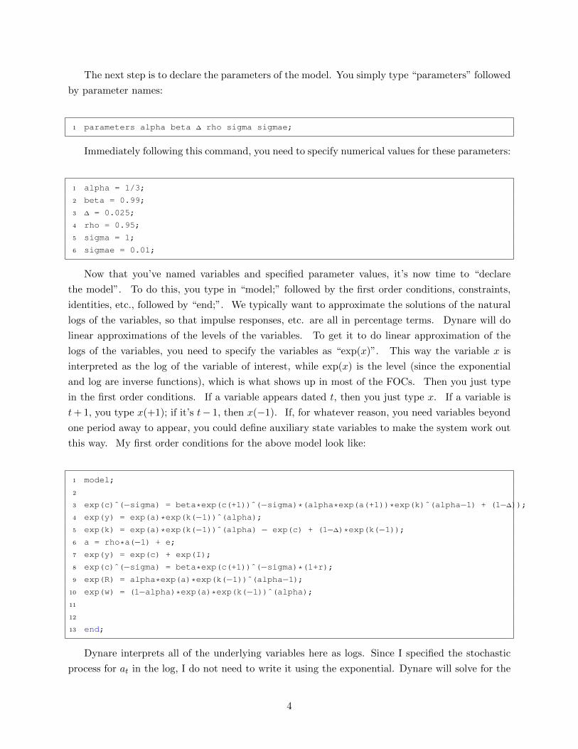
The next step is to declare the parameters of the model. You simply type “parameters” followed

by parameter names:

1 parameters alpha beta ∆ rho sigma sigmae;

Immediately following this command, you need to specify numerical values for these parameters:

1 alpha = 1/3;

2 beta = 0.99;

3 ∆ = 0.025;

4 rho = 0.95;

5 sigma = 1;

6 sigmae = 0.01;

Now that you’ve named variables and specified parameter values, it’s now time to “declare

the model”. To do this, you type in “model;” followed by the first order conditions, constraints,

identities, etc., followed by “end;”. We typically want to approximate the solutions of the natural

logs of the variables, so that impulse responses, etc. are all in percentage terms. Dynare will do

linear approximations of the levels of the variables. To get it to do linear approximation of the

logs of the variables, you need to specify the variables as “exp(x)”. This way the variable x is

interpreted as the log of the variable of interest, while exp(x) is the level (since the exponential

and log are inverse functions), which is what shows up in most of the FOCs. Then you just type

in the first order conditions. If a variable appears dated t, then you just type x. If a variable is

t+ 1, you type x(+1); if it’s t− 1, then x(−1). If, for whatever reason, you need variables beyond

one period away to appear, you could define auxiliary state variables to make the system work out

this way. My first order conditions for the above model look like:

1 model;

2

3 exp(c)ˆ(−sigma) = beta*exp(c(+1))ˆ(−sigma)*(alpha*exp(a(+1))*exp(k)ˆ(alpha−1) + (1−∆));

4 exp(y) = exp(a)*exp(k(−1))ˆ(alpha);5 exp(k) = exp(a)*exp(k(−1))ˆ(alpha) − exp(c) + (1−∆)*exp(k(−1));6 a = rho*a(−1) + e;

7 exp(y) = exp(c) + exp(I);

8 exp(c)ˆ(−sigma) = beta*exp(c(+1))ˆ(−sigma)*(1+r);9 exp(R) = alpha*exp(a)*exp(k(−1))ˆ(alpha−1);

10 exp(w) = (1−alpha)*exp(a)*exp(k(−1))ˆ(alpha);11

12

13 end;

Dynare interprets all of the underlying variables here as logs. Since I specified the stochastic

process for at in the log, I do not need to write it using the exponential. Dynare will solve for the

4

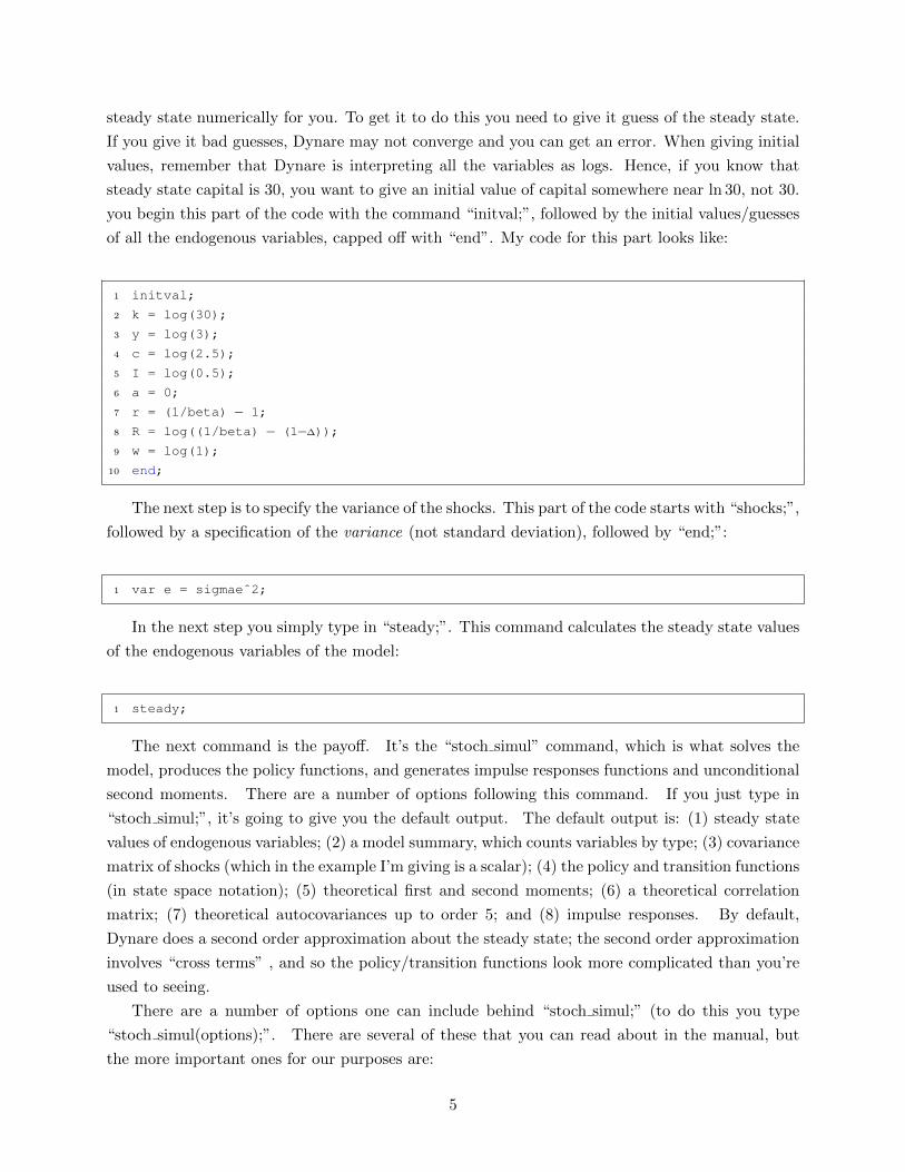
steady state numerically for you. To get it to do this you need to give it guess of the steady state.

If you give it bad guesses, Dynare may not converge and you can get an error. When giving initial

values, remember that Dynare is interpreting all the variables as logs. Hence, if you know that

steady state capital is 30, you want to give an initial value of capital somewhere near ln 30, not 30.

you begin this part of the code with the command “initval;”, followed by the initial values/guesses

of all the endogenous variables, capped off with “end”. My code for this part looks like:

1 initval;

2 k = log(30);

3 y = log(3);

4 c = log(2.5);

5 I = log(0.5);

6 a = 0;

7 r = (1/beta) − 1;

8 R = log((1/beta) − (1−∆));

9 w = log(1);

10 end;

The next step is to specify the variance of the shocks. This part of the code starts with “shocks;”,

followed by a specification of the variance (not standard deviation), followed by “end;”:

1 var e = sigmaeˆ2;

In the next step you simply type in “steady;”. This command calculates the steady state values

of the endogenous variables of the model:

1 steady;

The next command is the payoff. It’s the “stoch simul” command, which is what solves the

model, produces the policy functions, and generates impulse responses functions and unconditional

second moments. There are a number of options following this command. If you just type in

“stoch simul;”, it’s going to give you the default output. The default output is: (1) steady state

values of endogenous variables; (2) a model summary, which counts variables by type; (3) covariance

matrix of shocks (which in the example I’m giving is a scalar); (4) the policy and transition functions

(in state space notation); (5) theoretical first and second moments; (6) a theoretical correlation

matrix; (7) theoretical autocovariances up to order 5; and (8) impulse responses. By default,

Dynare does a second order approximation about the steady state; the second order approximation

involves “cross terms” , and so the policy/transition functions look more complicated than you’re

used to seeing.

There are a number of options one can include behind “stoch simul;” (to do this you type

“stoch simul(options);”. There are several of these that you can read about in the manual, but

the more important ones for our purposes are:

5

hp filter = integer: this will produce theoretical moments (variances, covariances, autocor-

relations) after HP filtering the data (the default is to apply no filter to the data). We

typically want to look at HP filtered moments, so this is an option you’ll want to use. The

integer is a number (i.e. 1600) corresponding to the penalty parameter in the HP filter. So,

for example, typing “stoch simul(hp filter=1600);” will produce theoretical (i.e. analytical)

moments of the HP filtered data. The only problem here is that it will not simultaneously do

HP filtering of simulated data; you can either get moments from simulated data or analytical

HP filtered moments

irf = integer: this will change the number of periods plotted in the impulse response functions.

The default value is 40. To suppress printing impulse responses altogether, type in 0 for

the number of horizons. For example, to see impulse responses for only 20 periods, type

“stoch simul(irf=20);”.

nocorr: this will mean it will not print a matrix of correlations in the command window

nofunctions: this will suppress printing the state space coefficients of the solution in the

command window

nomoments: this will suppress printing of moments

noprint: this will suppress printing of any output at all

order = 1, 2, or 3: this tells Dynare the order of the (log) approximation. The default is a

second order approximation. Hence, typing “order=1” will have it do a linear approximation.

periods = integer: Dynare’s default is to produce analytical/theoretical moments of the vari-

ables. Having periods not equal to zero will instead have it simulate data and take the

moments from the simulated data. By default, Dynare drops the first 100 values from a

simulation, so you need to give it a number of periods greater than 100 for this to work.

Hence, typing “stoch simul(periods=300);” will produce moments based on a simulation with

200 variables.

drop = integer: You can change the number of observations to drop from the simulations.

For example, typing “stoch simul(drop=0);” will result in no observations being dropped in

the simulations.

simul seed = integer: sets the seed used in the random number generator for the simulations.

For example, typing “stoch simul(nofunctions,hp filter=1600,order=1,irf=20);” will suppress

the policy function output, will produce analytical HP filtered moments, will do a first order

approximation, and will plot 20 periods in the impulse responses.

Dynare will produce policy and transition functions for the endogenous variables of the model

in state space form. Letting st be a m× 1 vector of states (here m = 2) and xt be a n× 1 vector

6

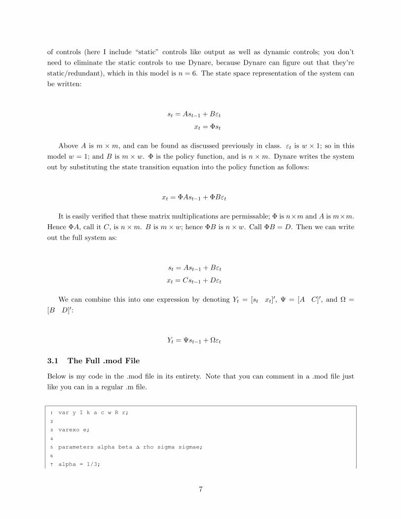
of controls (here I include “static” controls like output as well as dynamic controls; you don’t

need to eliminate the static controls to use Dynare, because Dynare can figure out that they’re

static/redundant), which in this model is n = 6. The state space representation of the system can

be written:

st = Ast−1 +Bεt

xt = Φst

Above A is m ×m, and can be found as discussed previously in class. εt is w × 1; so in this

model w = 1; and B is m × w. Φ is the policy function, and is n ×m. Dynare writes the system

out by substituting the state transition equation into the policy function as follows:

xt = ΦAst−1 + ΦBεt

It is easily verified that these matrix multiplications are permissable; Φ is n×m and A is m×m.

Hence ΦA, call it C, is n×m. B is m× w; hence ΦB is n× w. Call ΦB = D. Then we can write

out the full system as:

st = Ast−1 +Bεt

xt = Cst−1 +Dεt

We can combine this into one expression by denoting Yt = [st xt]′, Ψ = [A C]′, and Ω =

[B D]′:

Yt = Ψst−1 + Ωεt

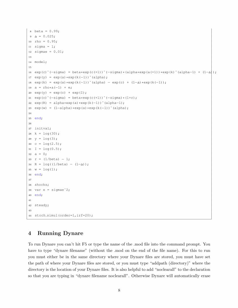
3.1 The Full .mod File

Below is my code in the .mod file in its entirety. Note that you can comment in a .mod file just

like you can in a regular .m file.


2

3 varexo e;

4


6

7 alpha = 1/3;

7

8 beta = 0.99;

9 ∆ = 0.025;

10 rho = 0.95;

11 sigma = 1;

12 sigmae = 0.01;

13

14 model;

15


17 exp(y) = exp(a)*exp(k(−1))ˆ(alpha);18 exp(k) = exp(a)*exp(k(−1))ˆ(alpha) − exp(c) + (1−∆)*exp(k(−1));19 a = rho*a(−1) + e;


21 exp(c)ˆ(−sigma) = beta*exp(c(+1))ˆ(−sigma)*(1+r);22 exp(R) = alpha*exp(a)*exp(k(−1))ˆ(alpha−1);23 exp(w) = (1−alpha)*exp(a)*exp(k(−1))ˆ(alpha);24

25 end;

26

27 initval;

28 k = log(30);

29 y = log(3);

30 c = log(2.5);

31 I = log(0.5);

32 a = 0;

33 r = (1/beta) − 1;

34 R = log((1/beta) − (1−∆));

35 w = log(1);

36 end;

37

38 shocks;


40 end;

41

42 steady;

43

44 stoch simul(order=1,irf=20);

4 Running Dynare

To run Dynare you can’t hit F5 or type the name of the .mod file into the command prompt. You

have to type “dynare filename” (without the .mod on the end of the file name). For this to run

you must either be in the same directory where your Dynare files are stored, you must have set

the path of where your Dynare files are stored, or you must type “addpath (directory)” where the

directory is the location of your Dynare files. It is also helpful to add “noclearall” to the declaration

so that you are typing in “dynare filename noclearall”. Otherwise Dynare will automatically erase

8

all previous output, which you may not want. Another option I often include is “nolog” which tells

Dynare to not produce a “log” file. I have found in the past that the creation of log files can cause

crashes when you’re doing loops.

So as to do other things, I usually write a .m file to go along with my .mod file. My code for

the .m file is simple:

1 clear all;

2 close all;

3

4 % execute a Dynare file

5

6 % specify parameters

7

8 beta = 0.99;

9 alpha = 1/3;

10 sigma = 1;

11 sigmae = 0.01;

12 rho = 0.9;

13 ∆ = 0.025;

14

15 save param nc alpha beta ∆ rho sigma sigmae

16

17 dynare basic nc dynare alt noclearall nolog

Here I’m saving the parameters as a .mat file. Dynare allows you to do this, and you can modify

the .mod file (as below) to accommodate this. This is particularly useful if you want to produce

moments for different parameter configurations that you might want to loop over.


2

3 varexo e;

4


6

7 load param nc;

8 set param value('alpha',alpha);

9 set param value('beta',beta);

10 set param value('sigma',sigma);

11 set param value('∆',∆);

12 set param value('rho',rho);

13 set param value('sigmae',sigmae);

14

15 model;

16


18 exp(y) = exp(a)*exp(k(−1))ˆ(alpha);

9

19 exp(k) = exp(a)*exp(k(−1))ˆ(alpha) − exp(c) + (1−∆)*exp(k(−1));20 a = rho*a(−1) + e;


22 exp(c)ˆ(−sigma) = beta*exp(c(+1))ˆ(−sigma)*(1+r);23 exp(R) = alpha*exp(a)*exp(k(−1))ˆ(alpha−1);24 exp(w) = (1−alpha)*exp(a)*exp(k(−1))ˆ(alpha);25

26 end;

27

28 initval;

29 k = log(30);

30 y = log(3);

31 c = log(2.5);

32 I = log(0.5);

33 a = 0;

34 r = (1/beta) − 1;

35 R = log((1/beta) − (1−∆));

36 w = log(1);

37 end;

38

39 shocks;


41 end;

42

43 steady;

44

45 stoch simul(order=1,irf=20);

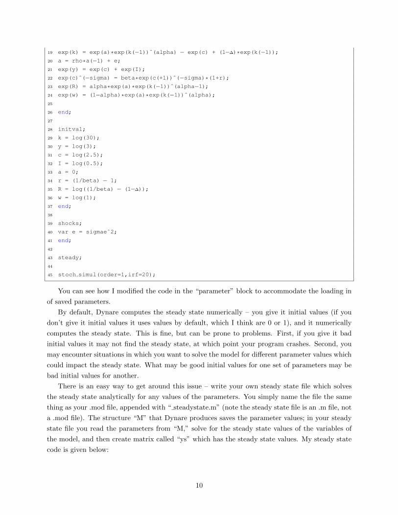
You can see how I modified the code in the “parameter” block to accommodate the loading in

of saved parameters.

By default, Dynare computes the steady state numerically – you give it initial values (if you

don’t give it initial values it uses values by default, which I think are 0 or 1), and it numerically

computes the steady state. This is fine, but can be prone to problems. First, if you give it bad

initial values it may not find the steady state, at which point your program crashes. Second, you

may encounter situations in which you want to solve the model for different parameter values which

could impact the steady state. What may be good initial values for one set of parameters may be

bad initial values for another.

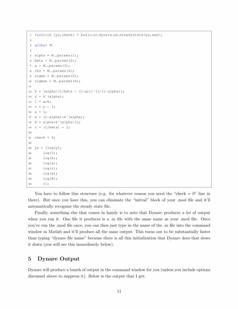
There is an easy way to get around this issue – write your own steady state file which solves

the steady state analytically for any values of the parameters. You simply name the file the same

thing as your .mod file, appended with “ steadystate.m” (note the steady state file is an .m file, not

a .mod file). The structure “M” that Dynare produces saves the parameter values; in your steady

state file you read the parameters from “M,” solve for the steady state values of the variables of

the model, and then create matrix called “ys” which has the steady state values. My steady state

code is given below:

10

1 function [ys,check] = basic nc dynare ss steadystate(ys,exe);

2

3 global M

4

5 alpha = M .params(1);

6 beta = M .params(2);

7 ∆ = M .params(3);

8 rho = M .params(4);

9 sigma = M .params(5);

10 sigmae = M .params(6);

11

12 k = (alpha/(1/beta − (1−∆)))ˆ(1/(1−alpha));13 y = kˆ(alpha);

14 I = ∆*k;

15 c = y − I;

16 a = 1;

17 w = (1−alpha)*kˆ(alpha);18 R = alpha*kˆ(alpha−1);19 r = (1/beta) − 1;

20

21 check = 0;

22

23 ys = [log(y);

24 log(I);

25 log(k);

26 log(a);

27 log(c);

28 log(w);

29 log(R);

30 r];

You have to follow this structure (e.g. for whatever reason you need the “check = 0” line in

there). But once you have this, you can eliminate the “initval” block of your .mod file and it’ll

automatically recognize the steady state file.

Finally, something else that comes in handy is to note that Dynare produces a lot of output

when you run it. One file it produces is a .m file with the same name as your .mod file. Once

you’ve run the .mod file once, you can then just type in the name of the .m file into the command

window in Matlab and it’ll produce all the same output. This turns out to be substantially faster

than typing “dynare file name” because there is all this initialization that Dynare does that slows

it down (you will see this immediately below).

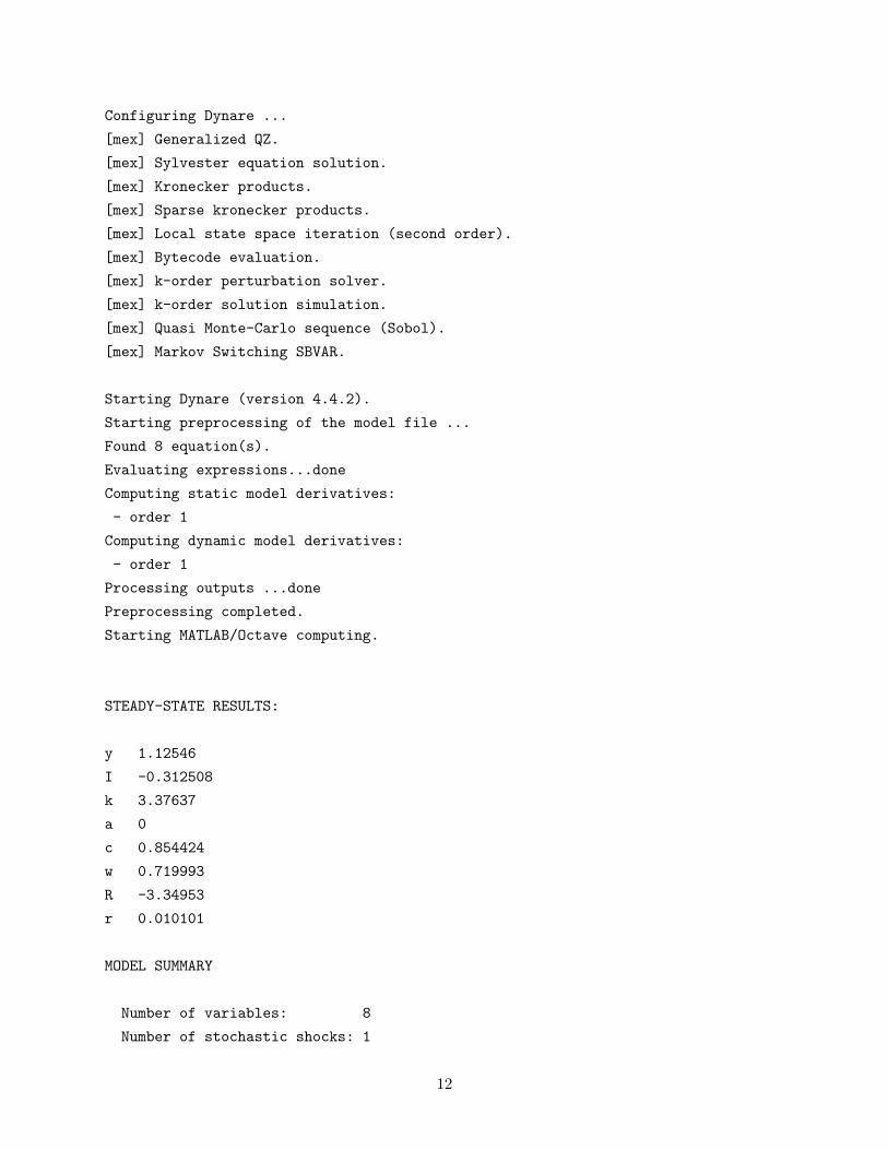
5 Dynare Output

Dynare will produce a bunch of output in the command window for you (unless you include options

discussed above to suppress it). Below is the output that I get:

11

Configuring Dynare ...

[mex] Generalized QZ.

[mex] Sylvester equation solution.

[mex] Kronecker products.

[mex] Sparse kronecker products.

[mex] Local state space iteration (second order).

[mex] Bytecode evaluation.

[mex] k-order perturbation solver.

[mex] k-order solution simulation.

[mex] Quasi Monte-Carlo sequence (Sobol).

[mex] Markov Switching SBVAR.

Starting Dynare (version 4.4.2).

Starting preprocessing of the model file ...

Found 8 equation(s).

Evaluating expressions...done

Computing static model derivatives:

- order 1

Computing dynamic model derivatives:

- order 1

Processing outputs ...done

Preprocessing completed.

Starting MATLAB/Octave computing.

STEADY-STATE RESULTS:

y 1.12546

I -0.312508

k 3.37637

a 0

c 0.854424

w 0.719993

R -3.34953

r 0.010101

MODEL SUMMARY

Number of variables: 8

Number of stochastic shocks: 1

12

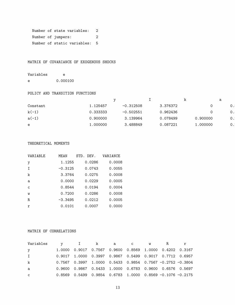
Number of state variables: 2

Number of jumpers: 2

Number of static variables: 5

MATRIX OF COVARIANCE OF EXOGENOUS SHOCKS

Variables e

e 0.000100

POLICY AND TRANSITION FUNCTIONS

y I k a c w R r

Constant 1.125457 -0.312508 3.376372 0 0.854424 0.719993 -3.349525 0.010101

k(-1) 0.333333 -0.502551 0.962436 0 0.593561 0.333333 -0.666666 -0.022522

a(-1) 0.900000 3.139964 0.078499 0.900000 0.202651 0.899999 0.899999 0.026595

e 1.000000 3.488849 0.087221 1.000000 0.225168 0.999999 0.999999 0.029550

THEORETICAL MOMENTS

VARIABLE MEAN STD. DEV. VARIANCE

y 1.1255 0.0286 0.0008

I -0.3125 0.0743 0.0055

k 3.3764 0.0275 0.0008

a 0.0000 0.0229 0.0005

c 0.8544 0.0194 0.0004

w 0.7200 0.0286 0.0008

R -3.3495 0.0212 0.0005

r 0.0101 0.0007 0.0000

MATRIX OF CORRELATIONS

Variables y I k a c w R r

y 1.0000 0.9017 0.7567 0.9600 0.8569 1.0000 0.4202 0.3167

I 0.9017 1.0000 0.3997 0.9867 0.5499 0.9017 0.7712 0.6957

k 0.7567 0.3997 1.0000 0.5433 0.9854 0.7567 -0.2752 -0.3804

a 0.9600 0.9867 0.5433 1.0000 0.6783 0.9600 0.6576 0.5697

c 0.8569 0.5499 0.9854 0.6783 1.0000 0.8569 -0.1076 -0.2175

13

w 1.0000 0.9017 0.7567 0.9600 0.8569 1.0000 0.4202 0.3167

R 0.4202 0.7712 -0.2752 0.6576 -0.1076 0.4202 1.0000 0.9938

r 0.3167 0.6957 -0.3804 0.5697 -0.2175 0.3167 0.9938 1.0000

COEFFICIENTS OF AUTOCORRELATION

Order 1 2 3 4 5

y 0.9367 0.8784 0.8246 0.7748 0.7289

I 0.8827 0.7777 0.6839 0.6001 0.5252

k 0.9980 0.9925 0.9840 0.9730 0.9597

a 0.9000 0.8100 0.7290 0.6561 0.5905

c 0.9927 0.9826 0.9702 0.9559 0.9398

w 0.9367 0.8784 0.8246 0.7748 0.7289

R 0.8768 0.7668 0.6686 0.5811 0.5031

r 0.8868 0.7853 0.6945 0.6133 0.5406

Total computing time : 0h00m01s

Several comments on the nature of the output. First, Dynare starts with a “model summary.”

This includes variables by “type” but note that the types (what Dynare calls states, jumpers, and

static) do not necessarily sum to the total number of variables. Dynare counts things which show

up in the equilibrium conditions just dated t as static variables; things which show up with a t− 1

as states, and things which show up with a t+ 1 as jumpers. Something could show up as both a

state and a jumper – here, a appears lagged (as a state) and with a “+1” in the Euler equation

(jumper).

The next part of the Dynare output are the policy and transition functions. The “constant”

in the policy and transition functions output is just the steady state values; the coefficients of

the (modified) state space representation are easy to understand. In addition, Dynare produces

means (steady state values), volatilities (standard deviations), and variances for each endogenous

variable. It also produces the matrix of correlations as well as coefficients of autocorrelation at

different lags. If there are multiple shocks, it will also produce a variance decomposition telling you

how important each shock is – using the terminology I’ve used, this is an “unconditional” variance

decomposition in the sense of showing the fraction of the total variance of each variable Given the

options I specified, all of these moments are theoretical (in the sense of being analytical, not based

on a simulation).

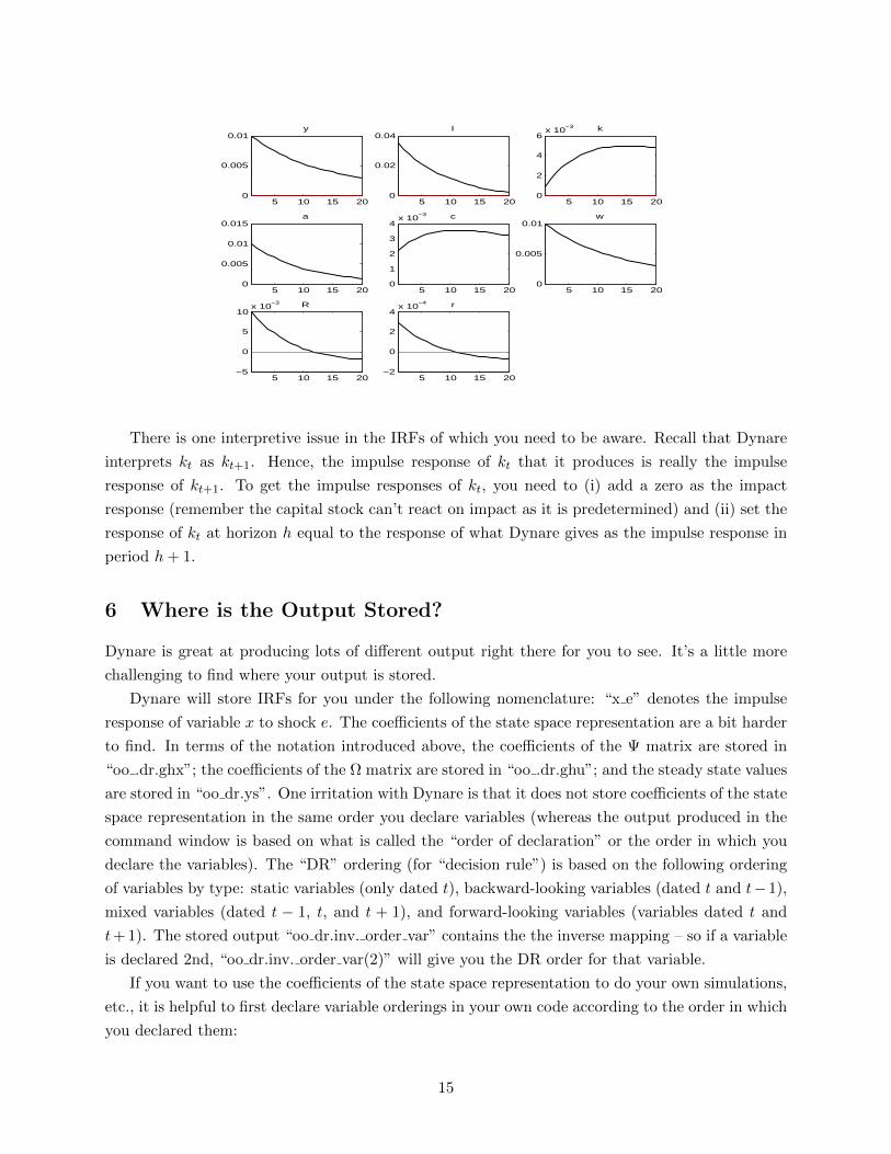
Dynare also produces impulse responses to the shocks. These are shown here:

14

5 10 15 200

0.005

0.01y

5 10 15 200

0.02

0.04I

5 10 15 200

2

4

6x 10

−3 k

5 10 15 200

0.005

0.01

0.015a

5 10 15 200

1

2

3

4x 10

−3 c

5 10 15 200

0.005

0.01w

5 10 15 20−5

0

5

10x 10

−3 R

5 10 15 20−2

0

2

4x 10

−4 r

There is one interpretive issue in the IRFs of which you need to be aware. Recall that Dynare

interprets kt as kt+1. Hence, the impulse response of kt that it produces is really the impulse

response of kt+1. To get the impulse responses of kt, you need to (i) add a zero as the impact

response (remember the capital stock can’t react on impact as it is predetermined) and (ii) set the

response of kt at horizon h equal to the response of what Dynare gives as the impulse response in

period h+ 1.

6 Where is the Output Stored?

Dynare is great at producing lots of different output right there for you to see. It’s a little more

challenging to find where your output is stored.

Dynare will store IRFs for you under the following nomenclature: “x e” denotes the impulse

response of variable x to shock e. The coefficients of the state space representation are a bit harder

to find. In terms of the notation introduced above, the coefficients of the Ψ matrix are stored in

“oo .dr.ghx”; the coefficients of the Ω matrix are stored in “oo .dr.ghu”; and the steady state values

are stored in “oo dr.ys”. One irritation with Dynare is that it does not store coefficients of the state

space representation in the same order you declare variables (whereas the output produced in the

command window is based on what is called the “order of declaration” or the order in which you

declare the variables). The “DR” ordering (for “decision rule”) is based on the following ordering

of variables by type: static variables (only dated t), backward-looking variables (dated t and t−1),

mixed variables (dated t − 1, t, and t + 1), and forward-looking variables (variables dated t and

t+ 1). The stored output “oo dr.inv. order var” contains the the inverse mapping – so if a variable

is declared 2nd, “oo dr.inv. order var(2)” will give you the DR order for that variable.

If you want to use the coefficients of the state space representation to do your own simulations,

etc., it is helpful to first declare variable orderings in your own code according to the order in which

you declared them:

15

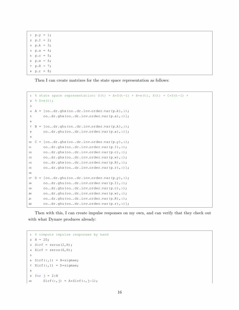
1 p y = 1;

2 p I = 2;

3 p k = 3;

4 p a = 4;

5 p c = 5;

6 p w = 6;

7 p R = 7;

8 p r = 8;

Then I can create matrixes for the state space representation as follows:

1 % state space representation: S(t) = A*S(t−1) + B*e(t), X(t) = C*S(t−1) +

2 % D*e(t);

3

4 A = [oo .dr.ghx(oo .dr.inv order var(p k),:);

5 oo .dr.ghx(oo .dr.inv order var(p a),:)];

6

7 B = [oo .dr.ghu(oo .dr.inv order var(p k),:);

8 oo .dr.ghu(oo .dr.inv order var(p a),:)];

9

10 C = [oo .dr.ghx(oo .dr.inv order var(p y),:);

11 oo .dr.ghx(oo .dr.inv order var(p I),:);

12 oo .dr.ghx(oo .dr.inv order var(p c),:);

13 oo .dr.ghx(oo .dr.inv order var(p w),:);

14 oo .dr.ghx(oo .dr.inv order var(p R),:);

15 oo .dr.ghx(oo .dr.inv order var(p r),:)];

16

17 D = [oo .dr.ghu(oo .dr.inv order var(p y),:);

18 oo .dr.ghu(oo .dr.inv order var(p I),:);

19 oo .dr.ghu(oo .dr.inv order var(p c),:);

20 oo .dr.ghu(oo .dr.inv order var(p w),:);

21 oo .dr.ghu(oo .dr.inv order var(p R),:);

22 oo .dr.ghu(oo .dr.inv order var(p r),:)];

Then with this, I can create impulse responses on my own, and can verify that they check out

with what Dynare produces already:

1 % compute impulse responses by hand

2 H = 20;

3 Sirf = zeros(2,H);

4 Xirf = zeros(6,H);

5

6 Sirf(:,1) = B*sigmae;

7 Xirf(:,1) = D*sigmae;

8

9 for j = 2:H

10 Sirf(:,j) = A*Sirf(:,j−1);

16

11 Xirf(:,j) = C*Sirf(:,j−1);12 end

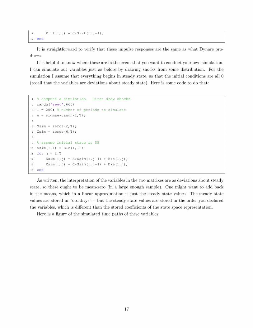
It is straightforward to verify that these impulse responses are the same as what Dynare pro-

duces.

It is helpful to know where these are in the event that you want to conduct your own simulation.

I can simulate out variables just as before by drawing shocks from some distribution. For the

simulation I assume that everything begins in steady state, so that the initial conditions are all 0

(recall that the variables are deviations about steady state). Here is some code to do that:

1 % compute a simulation. First draw shocks

2 randn('seed',666)

3 T = 200; % number of periods to simulate

4 e = sigmae*randn(1,T);

5

6 Ssim = zeros(2,T);

7 Xsim = zeros(6,T);

8

9 % assume initial state is SS

10 Ssim(:,1) = B*e(1,1);

11 for j = 2:T

12 Ssim(:,j) = A*Ssim(:,j−1) + B*e(1,j);

13 Xsim(:,j) = C*Ssim(:,j−1) + D*e(1,j);

14 end

As written, the interpretation of the variables in the two matrixes are as deviations about steady

state, so these ought to be mean-zero (in a large enough sample). One might want to add back

in the means, which in a linear approximation is just the steady state values. The steady state

values are stored in “oo .dr.ys” – but the steady state values are stored in the order you declared

the variables, which is different than the stored coefficients of the state space representation.

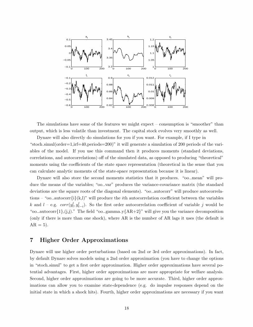
Here is a figure of the simulated time paths of these variables:

17

0 100 200−0.1

−0.05

0

0.05

0.1at

0 100 2003.3

3.35

3.4

3.45kt

0 100 2001

1.05

1.1

1.15

1.2yt

0 100 200−0.6

−0.5

−0.4

−0.3

−0.2

−0.1It

0 100 2000.82

0.84

0.86

0.88

0.9ct

0 100 2000.008

0.009

0.01

0.011

0.012rt

The simulations have some of the features we might expect – consumption is “smoother” than

output, which is less volatile than investment. The capital stock evolves very smoothly as well.

Dynare will also directly do simulations for you if you want. For example, if I type in

“stoch simul(order=1,irf=40,periods=200)” it will generate a simulation of 200 periods of the vari-

ables of the model. If you use this command then it produces moments (standard deviations,

correlations, and autocorrelations) off of the simulated data, as opposed to producing “theoretical”

moments using the coefficients of the state space representation (theoretical in the sense that you

can calculate analytic moments of the state-space representation because it is linear).

Dynare will also store the second moments statistics that it produces. “oo .mean” will pro-

duce the means of the variables; “oo .var” produces the variance-covariance matrix (the standard

deviations are the square roots of the diagonal elements). “oo .autocorr” will produce autocorrela-

tions – “oo .autocorri(k,l)” will produce the ith autocorrelation coefficient between the variables

k and l – e.g. corr(ylt, ylt−i). So the first order autocorrelation coefficient of variable j would be

“oo .autocorr1,(j,j).” The field “oo .gamma yAR+2” will give you the variance decomposition

(only if there is more than one shock), where AR is the number of AR lags it uses (the default is

AR = 5).

7 Higher Order Approximations

Dynare will use higher order perturbations (based on 2nd or 3rd order approximations). In fact,

by default Dynare solves models using a 2nd order approximation (you have to change the options

in “stoch simul” to get a first order approximation. Higher order approximations have several po-

tential advantages. First, higher order approximations are more appropriate for welfare analysis.

Second, higher order approximations are going to be more accurate. Third, higher order approx-

imations can allow you to examine state-dependence (e.g. do impulse responses depend on the

initial state in which a shock hits). Fourth, higher order approximations are necessary if you want

18

to think about “second moment” shocks (e.g. shocks to the variance of a shock . . . you actually

need a third order approximation for this to introduce interesting dynamics).

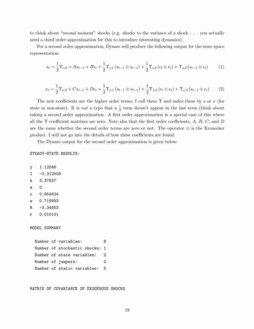
For a second order approximation, Dynare will produce the following output for the state space

representation:

st =1

2Υs,0 +Ast−1 +Bεt +

1

2Υs,1 (st−1 ⊗ st−1) +

1

2Υs,2 (εt ⊗ εt) + Υs,3 (st−1 ⊗ εt) (1)

xt =1

2Υx,0 + Cst−1 +Dεt +

1

2Υx,1 (st−1 ⊗ st−1) +

1

2Υx,2 (εt ⊗ εt) + Υx,3 (st−1 ⊗ εt) (2)

The new coefficients are the higher order terms; I call them Υ and index them by s or x (for

state or non-state). It is not a typo that a 12 term doesn’t appear in the last term (think about

taking a second order approximation. A first order approximation is a special case of this where

all the Υ coefficient matrixes are zero. Note also that the first order coefficients, A, B, C, and D

are the same whether the second order terms are zero or not. The operator ⊗ is the Kronecker

product. I will not go into the details of how these coefficients are found.

The Dynare output for the second order approximation is given below:


y 1.12546

I -0.312508

k 3.37637

a 0

c 0.854424

w 0.719993

R -3.34953

r 0.010101

MODEL SUMMARY







19

Variables e

e 0.000100


y I k a c w R r

Constant 1.125457 -0.312578 3.376370 0 0.854445 0.719993 -3.349525 0.010102

(correction) 0 -0.000070 -0.000002 0 0.000022 0 0 0.000001

k(-1) 0.333333 -0.502551 0.962436 0 0.593561 0.333333 -0.666666 -0.022522

a(-1) 0.900000 3.139964 0.078499 0.900000 0.202651 0.899999 0.899999 0.026595

e 1.000000 3.488849 0.087221 1.000000 0.225168 0.999999 0.999999 0.029550

k(-1),k(-1) 0 -0.536347 0.014107 0 0.024357 0 0 0.006895

a(-1),k(-1) 0 2.684454 -0.047889 0 -0.071355 0 0 -0.015943

a(-1),a(-1) 0 -3.408636 0.034945 0 0.037015 0 0 0.009257

e,e 0 -4.208192 0.043142 0 0.045698 0 0 0.011429

k(-1),e 0 2.982727 -0.053210 0 -0.079283 0 0 -0.017715

a(-1),e 0 -7.574746 0.077656 0 0.082257 0 0.000001 0.020572

APROXIMATED THEORETICAL MOMENTS


y 1.1256 0.0286 0.0008

I -0.3145 0.0743 0.0055

k 3.3768 0.0275 0.0008

a 0.0000 0.0229 0.0005

c 0.8547 0.0194 0.0004

w 0.7201 0.0286 0.0008

R -3.3498 0.0212 0.0005

r 0.0101 0.0007 0.0000

APPROXIMATED MATRIX OF CORRELATIONS

Variables y I k a c w R r

y 1.0000 0.9017 0.7567 0.9600 0.8569 1.0000 0.4202 0.3167

I 0.9017 1.0000 0.3997 0.9867 0.5499 0.9017 0.7712 0.6957

k 0.7567 0.3997 1.0000 0.5433 0.9854 0.7567 -0.2752 -0.3804

a 0.9600 0.9867 0.5433 1.0000 0.6783 0.9600 0.6576 0.5697

c 0.8569 0.5499 0.9854 0.6783 1.0000 0.8569 -0.1076 -0.2175

20

w 1.0000 0.9017 0.7567 0.9600 0.8569 1.0000 0.4202 0.3167

R 0.4202 0.7712 -0.2752 0.6576 -0.1076 0.4202 1.0000 0.9938

r 0.3167 0.6957 -0.3804 0.5697 -0.2175 0.3167 0.9938 1.0000

APPROXIMATED COEFFICIENTS OF AUTOCORRELATION

Order 1 2 3 4 5

y 0.9367 0.8784 0.8246 0.7748 0.7289

I 0.8827 0.7777 0.6839 0.6001 0.5252

k 0.9980 0.9925 0.9840 0.9730 0.9597

a 0.9000 0.8100 0.7290 0.6561 0.5905

c 0.9927 0.9826 0.9702 0.9559 0.9398

w 0.9367 0.8784 0.8246 0.7748 0.7289

R 0.8768 0.7668 0.6686 0.5811 0.5031

r 0.8868 0.7853 0.6945 0.6133 0.5406


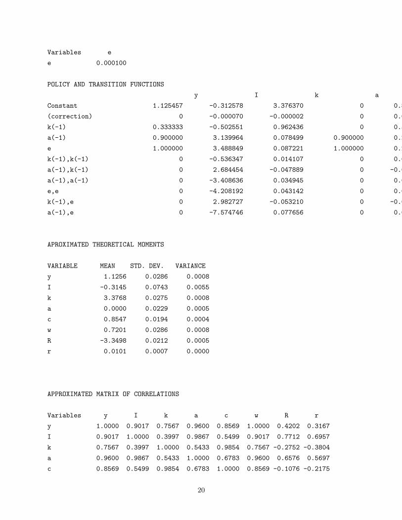
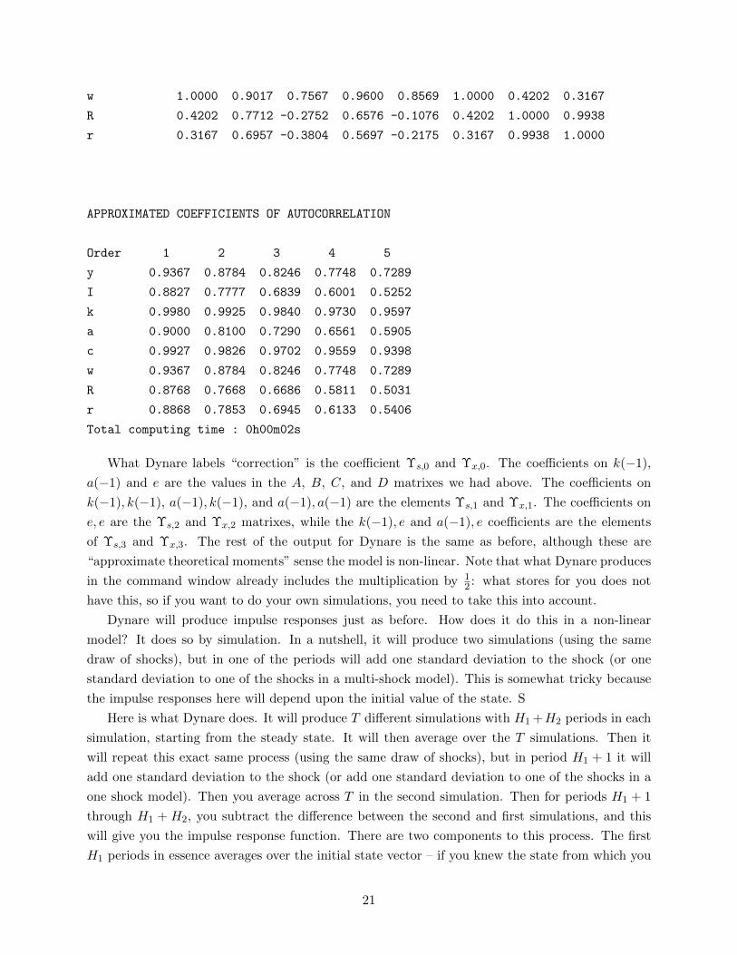
What Dynare labels “correction” is the coefficient Υs,0 and Υx,0. The coefficients on k(−1),

a(−1) and e are the values in the A, B, C, and D matrixes we had above. The coefficients on

k(−1), k(−1), a(−1), k(−1), and a(−1), a(−1) are the elements Υs,1 and Υx,1. The coefficients on

e, e are the Υs,2 and Υx,2 matrixes, while the k(−1), e and a(−1), e coefficients are the elements

of Υs,3 and Υx,3. The rest of the output for Dynare is the same as before, although these are

“approximate theoretical moments” sense the model is non-linear. Note that what Dynare produces

in the command window already includes the multiplication by 12 : what stores for you does not

have this, so if you want to do your own simulations, you need to take this into account.

Dynare will produce impulse responses just as before. How does it do this in a non-linear

model? It does so by simulation. In a nutshell, it will produce two simulations (using the same

draw of shocks), but in one of the periods will add one standard deviation to the shock (or one

standard deviation to one of the shocks in a multi-shock model). This is somewhat tricky because

the impulse responses here will depend upon the initial value of the state. S

Here is what Dynare does. It will produce T different simulations with H1 +H2 periods in each

simulation, starting from the steady state. It will then average over the T simulations. Then it

will repeat this exact same process (using the same draw of shocks), but in period H1 + 1 it will

add one standard deviation to the shock (or add one standard deviation to one of the shocks in a

one shock model). Then you average across T in the second simulation. Then for periods H1 + 1

through H1 + H2, you subtract the difference between the second and first simulations, and this

will give you the impulse response function. There are two components to this process. The first

H1 periods in essence averages over the initial state vector – if you knew the state from which you

21

wanted to start the impulse response function, you could set H1 = 0. In this sense what Dynare

produces are in a sense “average” impulse response. The second component is the typical approach

for simulating an impulse response function in a non-linear model.

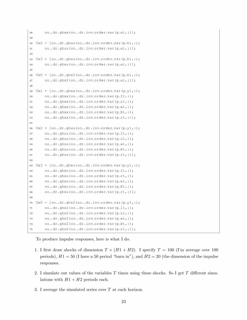
Dynare stores in the coefficients in a similar manner as in a first order approximation. I can

retrieve the A, B, C, and D matrixes as before. The Υs,1 and Υx,1 coefficients are stored in

“oo .dr.ghxx,” the Υs,2 and Υx,2 coefficients in “oo .dr.ghuu,” the Υs,3 and Υx,3 coefficients in

“oo .dr.ghxu,” and the Υs,0 and Υx,0 coefficients in “oo .dr.ghs2.” I retrieve the coefficients using

the code below:

1 [tn,sn] = size(oo .dr.ghx); % dimensions, tn is total number of variables,

2 % sn is number of states

3 A = zeros(sn,sn);

4 B = zeros(sn,1);

5 Us0 = zeros(sn,1);

6 Us1 = zeros(sn,snˆ2);

7 Us2 = zeros(sn,1);

8 Us3 = zeros(sn,sn*1); % 1 i the number of shocks

9

10 C = zeros(tn−sn,sn);11 D = zeros(tn−sn,1);12 Us0 = zeros(tn−sn,1);13 Us1 = zeros(tn−sn,snˆ2);14 Us2 = zeros(tn−sn,1);15 Us3 = zeros(tn−sn,sn*1); % 1 is the number of shocks

16

17 A = [oo .dr.ghx(oo .dr.inv order var(p k),:);

18 oo .dr.ghx(oo .dr.inv order var(p a),:)];

19

20 B = [oo .dr.ghu(oo .dr.inv order var(p k),:);

21 oo .dr.ghu(oo .dr.inv order var(p a),:)];

22

23 C = [oo .dr.ghx(oo .dr.inv order var(p y),:);

24 oo .dr.ghx(oo .dr.inv order var(p I),:);

25 oo .dr.ghx(oo .dr.inv order var(p c),:);

26 oo .dr.ghx(oo .dr.inv order var(p w),:);

27 oo .dr.ghx(oo .dr.inv order var(p R),:);

28 oo .dr.ghx(oo .dr.inv order var(p r),:)];

29

30 D = [oo .dr.ghu(oo .dr.inv order var(p y),:);

31 oo .dr.ghu(oo .dr.inv order var(p I),:);

32 oo .dr.ghu(oo .dr.inv order var(p c),:);

33 oo .dr.ghu(oo .dr.inv order var(p w),:);

34 oo .dr.ghu(oo .dr.inv order var(p R),:);

35 oo .dr.ghu(oo .dr.inv order var(p r),:)];

36

37 Us1 = [oo .dr.ghxx(oo .dr.inv order var(p k),:);

22

38 oo .dr.ghxx(oo .dr.inv order var(p a),:)];

39

40 Us2 = [oo .dr.ghuu(oo .dr.inv order var(p k),:);

41 oo .dr.ghuu(oo .dr.inv order var(p a),:)];

42

43 Us3 = [oo .dr.ghxu(oo .dr.inv order var(p k),:);

44 oo .dr.ghxu(oo .dr.inv order var(p a),:)];

45

46 Us0 = [oo .dr.ghs2(oo .dr.inv order var(p k),:);

47 oo .dr.ghs2(oo .dr.inv order var(p a),:)];

48

49 Ux1 = [oo .dr.ghxx(oo .dr.inv order var(p y),:);

50 oo .dr.ghxx(oo .dr.inv order var(p I),:);

51 oo .dr.ghxx(oo .dr.inv order var(p c),:);

52 oo .dr.ghxx(oo .dr.inv order var(p w),:);

53 oo .dr.ghxx(oo .dr.inv order var(p R),:);

54 oo .dr.ghxx(oo .dr.inv order var(p r),:)];

55

56 Ux2 = [oo .dr.ghuu(oo .dr.inv order var(p y),:);

57 oo .dr.ghuu(oo .dr.inv order var(p I),:);

58 oo .dr.ghuu(oo .dr.inv order var(p c),:);

59 oo .dr.ghuu(oo .dr.inv order var(p w),:);

60 oo .dr.ghuu(oo .dr.inv order var(p R),:);

61 oo .dr.ghuu(oo .dr.inv order var(p r),:)];

62

63 Ux3 = [oo .dr.ghxu(oo .dr.inv order var(p y),:);

64 oo .dr.ghxu(oo .dr.inv order var(p I),:);

65 oo .dr.ghxu(oo .dr.inv order var(p c),:);

66 oo .dr.ghxu(oo .dr.inv order var(p w),:);

67 oo .dr.ghxu(oo .dr.inv order var(p R),:);

68 oo .dr.ghxu(oo .dr.inv order var(p r),:)];

69

70 Ux0 = [oo .dr.ghs2(oo .dr.inv order var(p y),:);

71 oo .dr.ghs2(oo .dr.inv order var(p I),:);

72 oo .dr.ghs2(oo .dr.inv order var(p c),:);

73 oo .dr.ghs2(oo .dr.inv order var(p w),:);

74 oo .dr.ghs2(oo .dr.inv order var(p R),:);

75 oo .dr.ghs2(oo .dr.inv order var(p r),:)];

To produce impulse responses, here is what I do.

1. I first draw shocks of dimension T × (H1 + H2). I specify T = 100 (I’m average over 100

periods), H1 = 50 (I have a 50 period “burn in”), and H2 = 20 (the dimension of the impulse

responses.

2. I simulate out values of the variables T times using these shocks. So I get T different simu-

lations with H1 +H2 periods each.

3. I average the simulated series over T at each horizon.

23

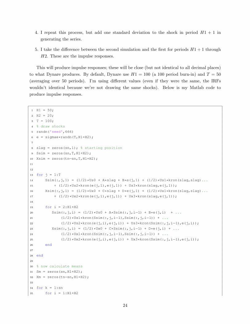
4. I repeat this process, but add one standard deviation to the shock in period H1 + 1 in

generating the series.

5. I take the difference between the second simulation and the first for periods H1 + 1 through

H2. These are the impulse responses.

This will produce impulse responses; these will be close (but not identical to all decimal places)

to what Dynare produces. By default, Dynare use H1 = 100 (a 100 period burn-in) and T = 50

(averaging over 50 periods). I’m using different values (even if they were the same, the IRFs

wouldn’t identical because we’re not drawing the same shocks). Below is my Matlab code to

produce impulse responses.

1 H1 = 50;

2 H2 = 20;

3 T = 100;

4 % draw shocks

5 randn('seed',666)

6 e = sigmae*randn(T,H1+H2);

7

8 slag = zeros(sn,1); % starting position

9 Ssim = zeros(sn,T,H1+H2);

10 Xsim = zeros(tn−sn,T,H1+H2);11

12

13 for j = 1:T

14 Ssim(:,j,1) = (1/2)*Us0 + A*slag + B*e(j,1) + (1/2)*Us1*kron(slag,slag)...

15 + (1/2)*Us2*kron(e(j,1),e(j,1)) + Us3*kron(slag,e(j,1));

16 Xsim(:,j,1) = (1/2)*Ux0 + C*slag + D*e(j,1) + (1/2)*Ux1*kron(slag,slag)...

17 + (1/2)*Ux2*kron(e(j,1),e(j,1)) + Ux3*kron(slag,e(j,1));

18

19 for i = 2:H1+H2

20 Ssim(:,j,i) = (1/2)*Us0 + A*Ssim(:,j,i−1) + B*e(j,i) + ...

21 (1/2)*Us1*kron(Ssim(:,j,i−1),Ssim(:,j,i−1)) + ...

22 (1/2)*Us2*kron(e(j,i),e(j,i)) + Us3*kron(Ssim(:,j,i−1),e(j,i));23 Xsim(:,j,i) = (1/2)*Ux0 + C*Ssim(:,j,i−1) + D*e(j,i) + ...

24 (1/2)*Ux1*kron(Ssim(:,j,i−1),Ssim(:,j,i−1)) + ...

25 (1/2)*Ux2*kron(e(j,i),e(j,i)) + Ux3*kron(Ssim(:,j,i−1),e(j,i));26 end

27

28 end

29

30 % now calculate means

31 Sm = zeros(sn,H1+H2);

32 Xm = zeros(tn−sn,H1+H2);33

34 for k = 1:sn

35 for i = 1:H1+H2

24

36 Sm(k,i) = mean(Ssim(k,:,i));

37 end

38 end

39

40 for k = 1:tn−sn41 for i = 1:H1+H2

42 Xm(k,i) = mean(Xsim(k,:,i));

43 end

44 end

45

46 % Now do a second simulation

47 Ssim2 = zeros(sn,T,H1+H2);

48 Xsim2 = zeros(tn−sn,T,H1+H2);49

50 % Keep e the same, but add sigmae to it in period H1+1

51 e1 = e;

52 e1(:,H1+1) = e1(:,H1+1) + sigmae;

53

54 % Now resimulate using e1

55 for j = 1:T

56 Ssim2(:,j,1) = (1/2)*Us0 + A*slag + B*e1(j,1) + ...

57 (1/2)*Us1*kron(slag,slag) + (1/2)*Us2*kron(e1(j,1),e1(j,1)) ...

58 + Us3*kron(slag,e1(j,1));

59 Xsim2(:,j,1) = (1/2)*Ux0 + C*slag + D*e1(j,1) + ...

60 (1/2)*Ux1*kron(slag,slag) + (1/2)*Ux2*kron(e1(j,1),e1(j,1)) + ...

61 Ux3*kron(slag,e1(j,1));

62

63 for i = 2:H1+H2

64 Ssim2(:,j,i) = (1/2)*Us0 + A*Ssim2(:,j,i−1) + B*e1(j,i) + ...

65 (1/2)*Us1*kron(Ssim2(:,j,i−1),Ssim2(:,j,i−1)) + ...

66 (1/2)*Us2*kron(e1(j,i),e1(j,i)) + ...

67 Us3*kron(Ssim2(:,j,i−1),e1(j,i));68 Xsim2(:,j,i) = (1/2)*Ux0 + C*Ssim2(:,j,i−1) + D*e1(j,i) + ...

69 (1/2)*Ux1*kron(Ssim2(:,j,i−1),Ssim2(:,j,i−1)) + ...

70 (1/2)*Ux2*kron(e1(j,i),e1(j,i)) + ...

71 Ux3*kron(Ssim2(:,j,i−1),e1(j,i));72 end

73

74 end

75


77 Sm2 = zeros(sn,H1+H2);

78 Xm2 = zeros(tn−sn,H1+H2);79

80 for k = 1:sn

81 for i = 1:H1+H2

82 Sm2(k,i) = mean(Ssim2(k,:,i));

83 end

84 end

25

85

86 for k = 1:tn−sn87 for i = 1:H1+H2

88 Xm2(k,i) = mean(Xsim2(k,:,i));

89 end

90 end

91

92 Sirf = zeros(sn,H2);

93 Xirf = zeros(tn−sn,H2);94

95 for j = 1:H2

96 Sirf(:,j) = Sm2(:,H1+j) − Sm(:,H1+j);

97 Xirf(:,j) = Xm2(:,H1+j) − Xm(:,H1+j);

98 end

An irritation sometimes arises here. Unlike in a first order approximation, higher order approx-

imations can explode. In a simple model like this explosion is unlikely for reasonably sized shocks,

but you can get the model to be explosive if you make the shocks big enough. In multi-shock

models explosion occurs somewhat more frequently.

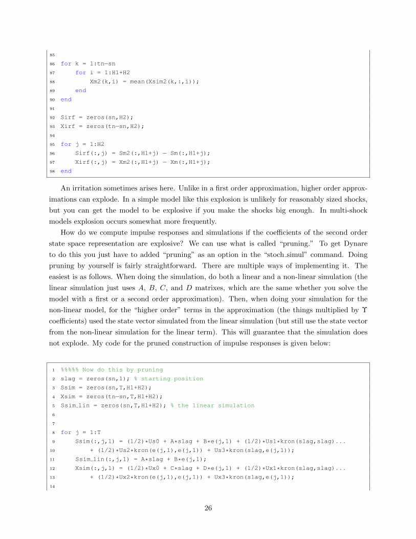
How do we compute impulse responses and simulations if the coefficients of the second order

state space representation are explosive? We can use what is called “pruning.” To get Dynare

to do this you just have to added “pruning” as an option in the “stoch simul” command. Doing

pruning by yourself is fairly straightforward. There are multiple ways of implementing it. The

easiest is as follows. When doing the simulation, do both a linear and a non-linear simulation (the

linear simulation just uses A, B, C, and D matrixes, which are the same whether you solve the

model with a first or a second order approximation). Then, when doing your simulation for the

non-linear model, for the “higher order” terms in the approximation (the things multiplied by Υ

coefficients) used the state vector simulated from the linear simulation (but still use the state vector

from the non-linear simulation for the linear term). This will guarantee that the simulation does

not explode. My code for the pruned construction of impulse responses is given below:

1 %%%%% Now do this by pruning

2 slag = zeros(sn,1); % starting position

3 Ssim = zeros(sn,T,H1+H2);

4 Xsim = zeros(tn−sn,T,H1+H2);5 Ssim lin = zeros(sn,T,H1+H2); % the linear simulation

6

7

8 for j = 1:T

9 Ssim(:,j,1) = (1/2)*Us0 + A*slag + B*e(j,1) + (1/2)*Us1*kron(slag,slag)...

10 + (1/2)*Us2*kron(e(j,1),e(j,1)) + Us3*kron(slag,e(j,1));

11 Ssim lin(:,j,1) = A*slag + B*e(j,1);

12 Xsim(:,j,1) = (1/2)*Ux0 + C*slag + D*e(j,1) + (1/2)*Ux1*kron(slag,slag)...

13 + (1/2)*Ux2*kron(e(j,1),e(j,1)) + Ux3*kron(slag,e(j,1));

14

26

15 for i = 2:H1+H2

16 Ssim(:,j,i) = (1/2)*Us0 + A*Ssim(:,j,i−1) + B*e(j,i) + ...

17 (1/2)*Us1*kron(Ssim lin(:,j,i−1),Ssim lin(:,j,i−1)) + ...

18 (1/2)*Us2*kron(e(j,i),e(j,i)) + Us3*kron(Ssim lin(:,j,i−1),e(j,i));19 Ssim lin(:,j,i) = A*Ssim lin(:,j,i−1) + B*e(j,i);

20 Xsim(:,j,i) = (1/2)*Ux0 + C*Ssim(:,j,i−1) + D*e(j,i) + ...

21 (1/2)*Ux1*kron(Ssim lin(:,j,i−1),Ssim lin(:,j,i−1)) + ...

22 (1/2)*Ux2*kron(e(j,i),e(j,i)) + Ux3*kron(Ssim lin(:,j,i−1),e(j,i));23 end

24

25 end

26


28 Sm = zeros(sn,H1+H2);

29 Xm = zeros(tn−sn,H1+H2);30

31 for k = 1:sn

32 for i = 1:H1+H2

33 Sm(k,i) = mean(Ssim(k,:,i));

34 end

35 end

36

37 for k = 1:tn−sn38 for i = 1:H1+H2

39 Xm(k,i) = mean(Xsim(k,:,i));

40 end

41 end

42

43 % Now do a second simulation

44 Ssim2 = zeros(sn,T,H1+H2);

45 Xsim2 = zeros(tn−sn,T,H1+H2);46 Ssim2 lin = zeros(sn,T,H1+H2);

47

48 % Keep e the same, but add sigmae to it in period H1+1

49 e1 = e;

50 e1(:,H1+1) = e1(:,H1+1) + sigmae;

51

52 % Now resimulate using e1

53 for j = 1:T

54 Ssim2(:,j,1) = (1/2)*Us0 + A*slag + B*e1(j,1) + ...

55 (1/2)*Us1*kron(slag,slag) + (1/2)*Us2*kron(e1(j,1),e1(j,1)) ...

56 + Us3*kron(slag,e1(j,1));

57 Ssim2 lin(:,j,1) = A*slag + B*e1(j,1);

58 Xsim2(:,j,1) = (1/2)*Ux0 + C*slag + D*e1(j,1) + ...

59 (1/2)*Ux1*kron(slag,slag) + (1/2)*Ux2*kron(e1(j,1),e1(j,1)) + ...

60 Ux3*kron(slag,e1(j,1));

61

62 for i = 2:H1+H2

63 Ssim2(:,j,i) = (1/2)*Us0 + A*Ssim2(:,j,i−1) + B*e1(j,i) + ...

27

64 (1/2)*Us1*kron(Ssim2 lin(:,j,i−1),Ssim2 lin(:,j,i−1)) + ...

65 (1/2)*Us2*kron(e1(j,i),e1(j,i)) + ...

66 Us3*kron(Ssim2 lin(:,j,i−1),e1(j,i));67 Ssim2 lin(:,j,i) = A*Ssim2 lin(:,j,i−1) + B*e1(j,i);

68 Xsim2(:,j,i) = (1/2)*Ux0 + C*Ssim2(:,j,i−1) + D*e1(j,i) + ...

69 (1/2)*Ux1*kron(Ssim2 lin(:,j,i−1),Ssim2 lin(:,j,i−1)) + ...

70 (1/2)*Ux2*kron(e1(j,i),e1(j,i)) + ...

71 Ux3*kron(Ssim2 lin(:,j,i−1),e1(j,i));72 end

73

74 end

75


77 Sm2 = zeros(sn,H1+H2);

78 Xm2 = zeros(tn−sn,H1+H2);79

80 for k = 1:sn

81 for i = 1:H1+H2

82 Sm2(k,i) = mean(Ssim2(k,:,i));

83 end

84 end

85

86 for k = 1:tn−sn87 for i = 1:H1+H2

88 Xm2(k,i) = mean(Xsim2(k,:,i));

89 end

90 end

91

92 Sirf prune = zeros(sn,H2);

93 Xirf prune = zeros(tn−sn,H2);94

95 for j = 1:H2

96 Sirf prune(:,j) = Sm2(:,H1+j) − Sm(:,H1+j);

97 Xirf prune(:,j) = Xm2(:,H1+j) − Xm(:,H1+j);

98 end

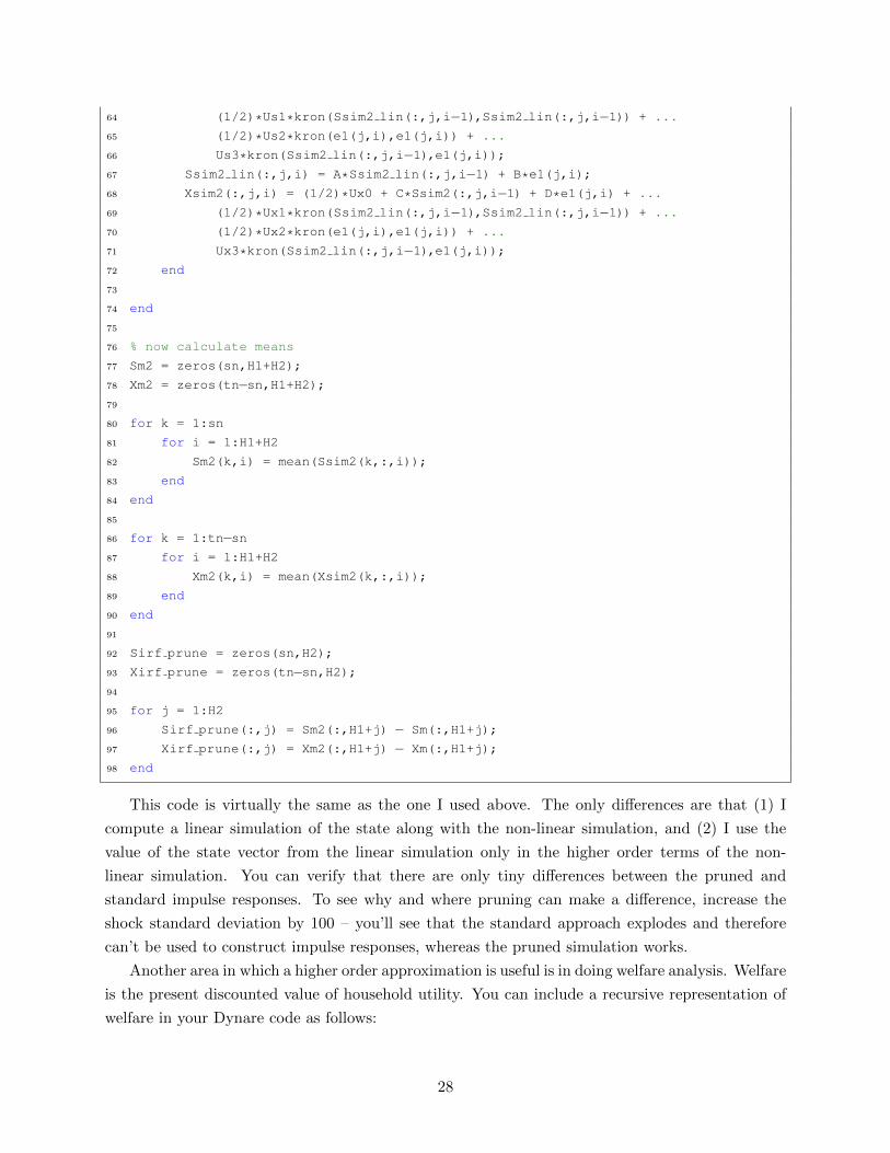
This code is virtually the same as the one I used above. The only differences are that (1) I

compute a linear simulation of the state along with the non-linear simulation, and (2) I use the

value of the state vector from the linear simulation only in the higher order terms of the non-

linear simulation. You can verify that there are only tiny differences between the pruned and

standard impulse responses. To see why and where pruning can make a difference, increase the

shock standard deviation by 100 – you’ll see that the standard approach explodes and therefore

can’t be used to construct impulse responses, whereas the pruned simulation works.

Another area in which a higher order approximation is useful is in doing welfare analysis. Welfare

is the present discounted value of household utility. You can include a recursive representation of

welfare in your Dynare code as follows:

28

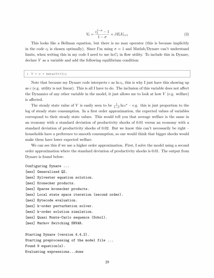
Vt =c1−σt − 1

1− σ+ βEtVt+1 (3)

This looks like a Bellman equation, but there is no max operator (this is because implicitly

in the code ct is chosen optimally). Since I’m using σ = 1 and Matlab/Dynare can’t understand

limits, when writing this in my code I need to use lnCt in flow utility. To include this in Dynare,

declare V as a variable and add the following equilibrium condition:

1 V = c + beta*V(+1);

Note that because my Dynare code interprets c as ln ct, this is why I just have this showing up

as c (e.g. utility is not linear). This is all I have to do. The inclusion of this variable does not affect

the Dynamics of any other variable in the model, it just allows me to look at how V (e.g. welfare)

is affected.

The steady state value of V is easily seen to be 11−β ln c∗ – e.g. this is just proportion to the

log of steady state consumption. In a first order approximation, the expected values of variables

correspond to their steady state values. This would tell you that average welfare is the same in

an economy with a standard deviation of productivity shocks of 0.01 versus an economy with a

standard deviation of productivity shocks of 0.02. But we know this can’t necessarily be right –

households have a preference to smooth consumption, so one would think that bigger shocks would

make them have lower expected welfare.

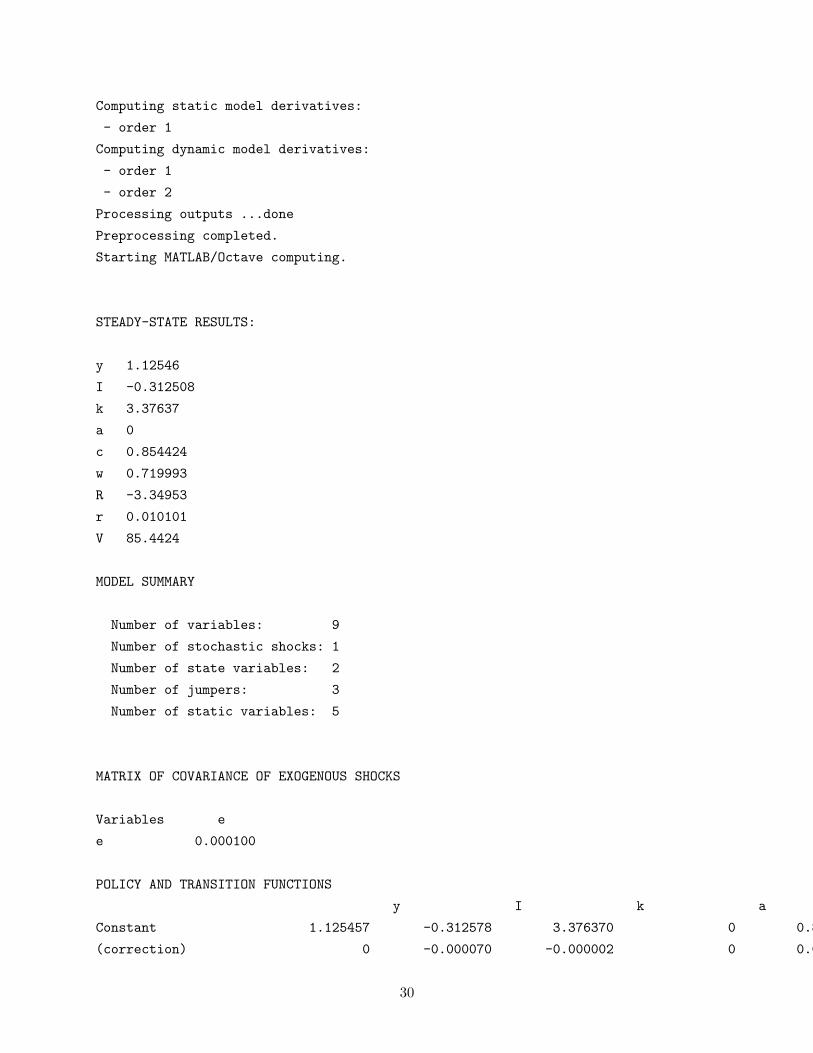
We can see this if we use a higher order approximation. First, I solve the model using a second

order approximation where the standard deviation of productivity shocks is 0.01. The output from

Dynare is found below:

Configuring Dynare ...

[mex] Generalized QZ.

[mex] Sylvester equation solution.

[mex] Kronecker products.

[mex] Sparse kronecker products.

[mex] Local state space iteration (second order).

[mex] Bytecode evaluation.

[mex] k-order perturbation solver.

[mex] k-order solution simulation.

[mex] Quasi Monte-Carlo sequence (Sobol).

[mex] Markov Switching SBVAR.

Starting Dynare (version 4.4.2).

Starting preprocessing of the model file ...

Found 9 equation(s).

Evaluating expressions...done

29

Computing static model derivatives:

- order 1

Computing dynamic model derivatives:

- order 1

- order 2

Processing outputs ...done

Preprocessing completed.

Starting MATLAB/Octave computing.


y 1.12546

I -0.312508

k 3.37637

a 0

c 0.854424

w 0.719993

R -3.34953

r 0.010101

V 85.4424

MODEL SUMMARY







Variables e

e 0.000100


y I k a c w R r V

Constant 1.125457 -0.312578 3.376370 0 0.854445 0.719993 -3.349525 0.010102 85.463106

(correction) 0 -0.000070 -0.000002 0 0.000022 0 0 0.000001 0.020737

30

k(-1) 0.333333 -0.502551 0.962436 0 0.593561 0.333333 -0.666666 -0.022522 12.578604

a(-1) 0.900000 3.139964 0.078499 0.900000 0.202651 0.899999 0.899999 0.026595 10.827396

e 1.000000 3.488849 0.087221 1.000000 0.225168 0.999999 0.999999 0.029550 12.030440

k(-1),k(-1) 0 -0.536347 0.014107 0 0.024357 0 0 0.006895 2.410514

a(-1),k(-1) 0 2.684454 -0.047889 0 -0.071355 0 0 -0.015943 -2.155674

a(-1),a(-1) 0 -3.408636 0.034945 0 0.037015 0 0 0.009257 1.696688

e,e 0 -4.208192 0.043142 0 0.045698 0 0 0.011429 2.094676

k(-1),e 0 2.982727 -0.053210 0 -0.079283 0 0 -0.017715 -2.395193

a(-1),e 0 -7.574746 0.077656 0 0.082257 0 0.000001 0.020572 3.770417

APROXIMATED THEORETICAL MOMENTS


y 1.1256 0.0286 0.0008

I -0.3145 0.0743 0.0055

k 3.3768 0.0275 0.0008

a -0.0000 0.0229 0.0005

c 0.8547 0.0194 0.0004

w 0.7201 0.0286 0.0008

R -3.3498 0.0212 0.0005

r 0.0101 0.0007 0.0000

V 85.4704 0.5380 0.2895

APPROXIMATED MATRIX OF CORRELATIONS

Variables y I k a c w R r V

y 1.0000 0.9017 0.7567 0.9600 0.8569 1.0000 0.4202 0.3167 0.9517

I 0.9017 1.0000 0.3997 0.9867 0.5499 0.9017 0.7712 0.6957 0.7254

k 0.7567 0.3997 1.0000 0.5433 0.9854 0.7567 -0.2752 -0.3804 0.9209

a 0.9600 0.9867 0.5433 1.0000 0.6783 0.9600 0.6576 0.5697 0.8276

c 0.8569 0.5499 0.9854 0.6783 1.0000 0.8569 -0.1076 -0.2175 0.9738

w 1.0000 0.9017 0.7567 0.9600 0.8569 1.0000 0.4202 0.3167 0.9517

R 0.4202 0.7712 -0.2752 0.6576 -0.1076 0.4202 1.0000 0.9938 0.1213

r 0.3167 0.6957 -0.3804 0.5697 -0.2175 0.3167 0.9938 1.0000 0.0102

V 0.9517 0.7254 0.9209 0.8276 0.9738 0.9517 0.1213 0.0102 1.0000

31

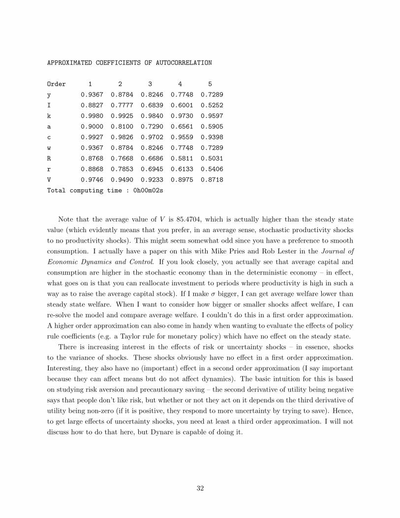
APPROXIMATED COEFFICIENTS OF AUTOCORRELATION

Order 1 2 3 4 5

y 0.9367 0.8784 0.8246 0.7748 0.7289

I 0.8827 0.7777 0.6839 0.6001 0.5252

k 0.9980 0.9925 0.9840 0.9730 0.9597

a 0.9000 0.8100 0.7290 0.6561 0.5905

c 0.9927 0.9826 0.9702 0.9559 0.9398

w 0.9367 0.8784 0.8246 0.7748 0.7289

R 0.8768 0.7668 0.6686 0.5811 0.5031

r 0.8868 0.7853 0.6945 0.6133 0.5406

V 0.9746 0.9490 0.9233 0.8975 0.8718


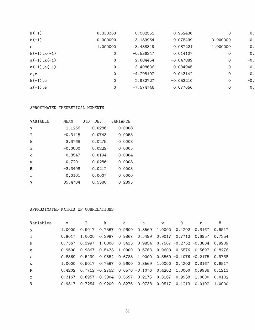
Note that the average value of V is 85.4704, which is actually higher than the steady state

value (which evidently means that you prefer, in an average sense, stochastic productivity shocks

to no productivity shocks). This might seem somewhat odd since you have a preference to smooth

consumption. I actually have a paper on this with Mike Pries and Rob Lester in the Journal of

Economic Dynamics and Control. If you look closely, you actually see that average capital and

consumption are higher in the stochastic economy than in the deterministic economy – in effect,

what goes on is that you can reallocate investment to periods where productivity is high in such a

way as to raise the average capital stock). If I make σ bigger, I can get average welfare lower than

steady state welfare. When I want to consider how bigger or smaller shocks affect welfare, I can

re-solve the model and compare average welfare. I couldn’t do this in a first order approximation.

A higher order approximation can also come in handy when wanting to evaluate the effects of policy

rule coefficients (e.g. a Taylor rule for monetary policy) which have no effect on the steady state.

There is increasing interest in the effects of risk or uncertainty shocks – in essence, shocks

to the variance of shocks. These shocks obviously have no effect in a first order approximation.

Interesting, they also have no (important) effect in a second order approximation (I say important

because they can affect means but do not affect dynamics). The basic intuition for this is based

on studying risk aversion and precautionary saving – the second derivative of utility being negative

says that people don’t like risk, but whether or not they act on it depends on the third derivative of

utility being non-zero (if it is positive, they respond to more uncertainty by trying to save). Hence,

to get large effects of uncertainty shocks, you need at least a third order approximation. I will not

discuss how to do that here, but Dynare is capable of doing it.

32

graduate macro theory ii: notes on using dynareesims1/using_dynare_sp15.pdf · graduate macro...

Documents