gramian-based model reduction (for linear and nonlinear systems)
TRANSCRIPT

Reduction de Modele a Base de Grammaires
pour Systeme Lineaire et Non Lineaire
Christian Himpe
38e Ecole Internationale d’ete de Controle AutomatiqueApproximation des Systemes Dynamiques a Grande Echelle
2017–09–11

Gramian-Based Model Reductionfor Linear and Nonlinear Systems
Christian Himpe
38th International Summer School of Automatic ControlApproximation of Large-Scale Dynamical Systems
2017–09–11
What is Model Reduction?
Given a differential equation model:
Algorithmic computation of simple surrogate models,
preserving essential features of the original model.
C. Himpe, [email protected] Gramian-Based Model Reduction 3/128
Why Model Reduction?
Enable computational simulation
Reduce numerical complexity
Multi-query / Many-query settings:
OptimizationControlSensitivity AnalysisUncertainty QuantificationComputer-Aided Design
Gain new insights
Surrogate modelling
C. Himpe, [email protected] Gramian-Based Model Reduction 4/128

Some Examples
Mechanical problems
Electrical circuits
Fluid dynamics
Inference of brain connectivity
Scenario analysis for gas networks1
1BMWi funded MathEnergy project.
C. Himpe, [email protected] Gramian-Based Model Reduction 5/128

Model Reduction Overview
Moment Matching
Transfer Function Interpolation
Matrix Interpolation
Hankel Norm Approximation
Proper Orthogonal Decomposition
Balanced Proper Orthgonal Decomposition
Balanced Truncation
Approximate Balancing
Singular Perturbation
Balanced Gains
Empirical Gramians
...
C. Himpe, [email protected] Gramian-Based Model Reduction 6/128

Gramian-Based Model Reduction
Encode relevant information about a system
in operators (matrices) with specific attributes,
which induce projections
to spaces with sorted components.
Truncated projections then
map to a meaningful subspace
inducing a reduced order model.
C. Himpe, [email protected] Gramian-Based Model Reduction 7/128

Outline
1. System-Theoretic Preliminaries
2. Linear Gramian-Based Model Reduction
3. Nonlinear Gramian-Based Model Reduction
4. Combined Reduction in Action
5. Other Uses for System Gramians
C. Himpe, [email protected] Gramian-Based Model Reduction 8/128

Review Papers
A.C. Antoulas, D.C. Sorensen, and S. Gugercin. A survey of modelreduction methods for large-scale systems. In Structured Matrices inMathematics, Computer Science, and Engineering I, ContemporaryMathematics, vol. 280: 193–219, 2001.
A.C. Antoulas. An overview of approximation methods for large-scaledynamical systems. Annual Reviews in Control, 29(2): 181–190, 2005.
U. Baur, P. Benner, and L. Feng. Model Order Reduction for Linear andNonlinear Systems: A System-Theoretic Perspective. Archives ofComputational Methods in Engineering, 21(4): 331–358, 2014.
P. Benner, S. Gugercin, and K. Willcox. A Survey of Projection-BasedModel Reduction Methods for Parametric Dynamical Systems. SIAMReviews, 57(4): 483–531, 2015.
C. Himpe. emgr - The Empirical Gramian Framework. arXiv e-print,cs.MS: 1611.00675, 2016.
C. Himpe, [email protected] Gramian-Based Model Reduction 9/128


MORwiki
Model Order Reduction Wiki:
http://modelreduction.org
Methods
Benchmarks
Software
Event Calendar
Comprehensive bib
C. Himpe, [email protected] Gramian-Based Model Reduction 11/128

Before We Start
The slides will be online.
Ask questions.
There is a hands-on lab session tomorrow!
C. Himpe, [email protected] Gramian-Based Model Reduction 12/128
Part I: System-Theoretic Preliminaries
1. Motivating Model Reduction
2. Dynamical Systems Summary
3. Basic System Theory
4. Generic Model Reduction
5. Principal Axis Transformation
C. Himpe, [email protected] Gramian-Based Model Reduction 13/128

Large-Scale Systems
Differential equation:
F (s, x ,Dαx) = 0
Multi-index differential operator: Dα = Dα1
1 . . .Dαnn .
Analytical solution: x(s).
Discrete approximate solution: xh(sh).
Large-Scale discretized dimension: dim(xh(sh))� 1.
Example: 1D heat equation: F (x , ∂2x∂s2 ).
C. Himpe, [email protected] Gramian-Based Model Reduction 14/128

Dynamical System
Continous dynamical system over R:
x(t) = f (t, x(t))
Time: t ∈ R+
State: x : R→ RN
State-space: RN , N <∞Vector field: f : R× RN → RN
Ordinary Differential Equation (ODE): x = ∂x∂t
Initial Value Problem (IVP): x0 = x(t0)
C. Himpe, [email protected] Gramian-Based Model Reduction 15/128

Fundamental Solution
Linear time invariant homogenous system of ODEs:
x(t) = Ax(t)
IVP Solution:
x(t) = eAt x0
Fundamental Solution:
L(·)(t) = eAt
System matrix: A ∈ RN×N
Matrix exponential: eA = exp(A) :=∑∞
k=01k!A
k
C. Himpe, [email protected] Gramian-Based Model Reduction 16/128
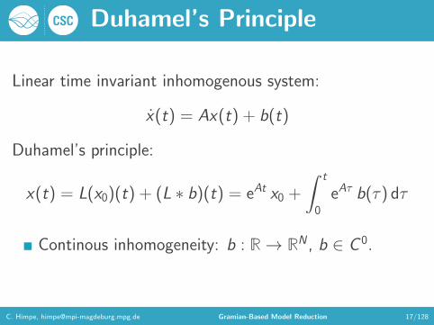
Duhamel’s Principle
Linear time invariant inhomogenous system:
x(t) = Ax(t) + b(t)
Duhamel’s principle:
x(t) = L(x0)(t) + (L ∗ b)(t) = eAt x0 +
∫ t
0
eAτ b(τ) dτ
Continous inhomogeneity: b : R→ RN , b ∈ C 0.
C. Himpe, [email protected] Gramian-Based Model Reduction 17/128

Lyapunov Stability
Stability:
‖x(t)‖ <∞,∀t > 0
Lyapunov stability:
∀ε > 0,∃δ > 0 : ‖x(t)− x‖ < ε,∀t ≥ 0,∀x0 : ‖x0 − x‖ < δ
Lyapunov stability (asymptotic):
∀ε > 0,∀δ > 0 : ‖x(t)− x‖ < ε,∀t ≥ T ,∀x0 : ‖x0 − x‖ < δ
Lyapunov stability (exponential):
∃c1, c2 ∈ R : ‖x(t)− x‖ < c1 e−c2t ‖x0 − x‖,∀t > 0
Steady state x : f (t, x) = 0
C. Himpe, [email protected] Gramian-Based Model Reduction 18/128
Linear Stability
Global stability via spectrum:
A ∈ RN×N Hurwitz
⇔ Re(λi(A)) < 0, i = 1 . . .N
⇔ x exponentially stable
⇔ x asymptotically stable
C. Himpe, [email protected] Gramian-Based Model Reduction 19/128

Nonlinear Stability
Local stability via linearization:
f ∈ C 1, x ∈ RN : f (x) = 0
→ A` :=∂f
∂x(x)
⇒ x`(t) = A`x`(t) ≈ f (x(t)), ‖x(t)− x‖ < ε
→ x` globally stable⇒ x locally stable
C. Himpe, [email protected] Gramian-Based Model Reduction 20/128

Control System
Nonlinear parametric control system:
x(t) = f (t, x(t), u(t), θ)
y(t) = g(t, x(t), u(t), θ)
Input: u : R→ RM
State: x : R→ RN
Output: y : R→ RQ
Parameter: θ ∈ RP
Vector field: f : R× RN × RM × RQ → RN
Output functional: g : R× RN × RM × RQ → RQ
C. Himpe, [email protected] Gramian-Based Model Reduction 21/128

Notation
Input dimension: M := dim(u(t)) <∞State dimension: N := dim(x(t)) <∞Output dimension: Q := dim(y(t)) <∞Parameter dimension: P := dim(θ) <∞
M = Q → Square system
M = Q = 1→ SISO system
M = 1,Q > 1→ SIMO system
M > 1,Q = 1→ MISO system
M > 1,Q > 1→ MIMO system
C. Himpe, [email protected] Gramian-Based Model Reduction 22/128

Linear Control System
Linear time-invariant (LTI) control system:
x(t) = Ax(t) + Bu(t)
y(t) = Cx(t) + Du(t)
System matrix: A ∈ RN×N
Input matrix: B ∈ RN×M
Output matrix: C ∈ RQ×N
Feed-forward matrix: D ∈ RQ×M
Here: Assume D = 0
C. Himpe, [email protected] Gramian-Based Model Reduction 23/128

Impulse Response
Impulse Input:
u(t) = δ(t) =
{∆−1 t < ∆
0 t ≥ ∆
LTI Impulse Response:
g(t) =
{C eAt B t ≥ 0
0 t < 0
Fundamental solution: y(t) = (g ∗ u)(t).∫∞0 δ(t) dt = 1
g(t < 0) = 0 ensures causality.
C. Himpe, [email protected] Gramian-Based Model Reduction 24/128

Bounded-Input-Bounded Output
Bounded-input-bounded-output (BIBO) stability:
‖u‖L∞ <∞→ ‖y‖L∞ <∞
Young’s Inequality2:
‖y‖L∞ = ‖g ∗ u‖L∞ < ‖g‖L1‖u‖L∞
‖g‖L1<∞⇒ BIBO stable
2W.H. Young. On the Multiplication of Successions of Fourier Constants.Proceedings of the Royal Society of London, Series A, 87(596): 331–339, 1912.
C. Himpe, [email protected] Gramian-Based Model Reduction 25/128

Adjoint System
Adjoint Operator:
〈y , g ∗ u〉 = 〈g ∗ y , u〉
⇒∫ ∞−∞
yᵀ(t)(∫ ∞−∞
C eA(t−τ) Bu(τ) dτ)
dt
=
∫ ∞−∞
uᵀ(t)(∫ ∞−∞
B eA(t−τ) Cy(t) dt)
dτ
=
∫ ∞−∞
uᵀ(t)(−∫ −∞∞
B e−A(τ−t) Cy(t) dt)
dτ
Adjoint System (backward running):
z(τ) = −Aᵀz(τ)− C ᵀy(τ)
u(τ) = Bᵀz(τ)
C. Himpe, [email protected] Gramian-Based Model Reduction 26/128

Transfer Function
Transfer function:
G (s) = C (1s − A)−1B
Properties:
Laplace transformation of the impulse response.
Rational function for LTI systems.
Frequency response G (s), for frequency s ∈ [0,∞).
C. Himpe, [email protected] Gramian-Based Model Reduction 27/128

System Symmetry
Symmetric System:
G (s) = (G (s))ᵀ
⇔ g(t) = (g(t))ᵀ
⇔ (CAkB) = (CAkB)ᵀ
⇔ ∃J = Jᵀ ∈ RN×N : AJ = JAᵀ, B = JC ᵀ
State-Space Symmetric System (J = 1):
A = Aᵀ, B = C ᵀ
All SISO systems are symmetric!
C. Himpe, [email protected] Gramian-Based Model Reduction 28/128
Model Reduction
Abstract Input-Output System:
u 7→ x 7→ y
Typical properties:
dim(x(t))� 1
dim(u(t))� dim(x(t))
dim(y(t))� dim(x(t))
Is there a shortcut?
C. Himpe, [email protected] Gramian-Based Model Reduction 29/128
Reduced Order Model
Generic Reduced Order Model:
xr(t) = fr(xr(t), u(t), θr)
yr(t) = gr(xr(t), u(t), θr)
xr(0) = xr ,0
Reduced State: xr : R→ Rn, n� N
Reduced Parameter: θr ∈ Rp, p � P
Approximate Output: yr : R→ RQ
Reduced Vector Field: fr : Rn × RM × Rp
Reduced Output Functional: gr : Rn × RM × Rp
C. Himpe, [email protected] Gramian-Based Model Reduction 30/128

Projections
Linear Projection:
V ∈ RN×N , V 2 = V
Truncated Projection:
rank(V ) < N ⇒ V ∼(V1 0
)Truncated projection: V1 ∈ Rn×N
Petrov-Galerkin: U1 ∈ RN×n, V1U1 = 1 ∈ Rn×n
Galerkin: U1 = V ᵀ1 , U1 orthogonal.
C. Himpe, [email protected] Gramian-Based Model Reduction 31/128

Projection-Based Model Reduction
Approximate Trajectory:
xr(t) := V1x(t)⇒ x(t) ≈ U1xr(t)
Reducing truncated projection: V1 ∈ Rn×N
Reconstructing truncated projection: U1 ∈ RN×n
Task: Find projections U1 and V1
C. Himpe, [email protected] Gramian-Based Model Reduction 32/128
State-Space Reduction
State-Space Reduced Model:
xr(t) = V1f (U1xr(t), u(t))
yr(t) = g(U1xr(t), u(t))
xr(0) = V1x0
Reduced vector field: fr := V1 ◦ f ◦ U1
Reduced output functional: gr := g ◦ U1
dim(xr(t))� dim(x(t))
‖y − yr‖ � 1
Requires evaluations of full order f , g !
C. Himpe, [email protected] Gramian-Based Model Reduction 33/128

Linear State-Space Reduction
Linear State-Space Reduced Model:
xr(t) = V1AU1xr + V1Bu(t) = Arxr(t) + Bru(t)
yr(t) = CU1xr(t) = Crxr(t)
xr(0) = V1x0
Linear Reduced Order Model:
Reduced system matrix: Ar ∈ Rn×n
Reduced input matrix: Br ∈ Rn×M
Reduced output matrix: Cr ∈ RQ×n
C. Himpe, [email protected] Gramian-Based Model Reduction 34/128

Affine State-Space Reduction
Affine State-Space Reduced Model:
xr(t) = V1f (x + U1xr(t), u(t))
yr(t) = g(x + U1xr(t), u(t))
xr(0) = V1(x0 − x)
x ∈ RN , often a steady state or mean.
x becomes perturbation from x .
Affine subspace usually better than linear subspace.
C. Himpe, [email protected] Gramian-Based Model Reduction 35/128
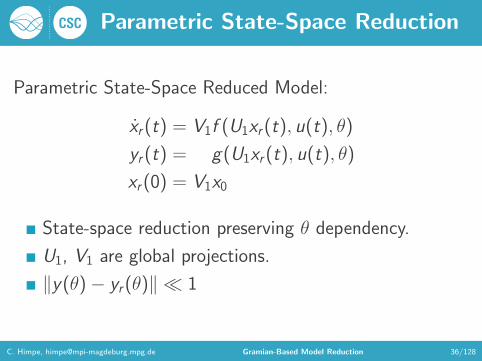
Parametric State-Space Reduction
Parametric State-Space Reduced Model:
xr(t) = V1f (U1xr(t), u(t), θ)
yr(t) = g(U1xr(t), u(t), θ)
xr(0) = V1x0
State-space reduction preserving θ dependency.
U1, V1 are global projections.
‖y(θ)− yr(θ)‖ � 1
C. Himpe, [email protected] Gramian-Based Model Reduction 36/128
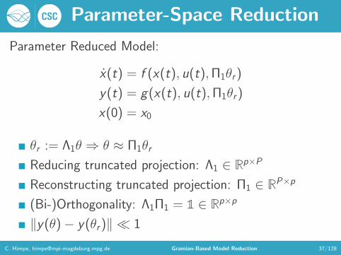
Parameter-Space Reduction
Parameter Reduced Model:
x(t) = f (x(t), u(t),Π1θr)
y(t) = g(x(t), u(t),Π1θr)
x(0) = x0
θr := Λ1θ ⇒ θ ≈ Π1θr
Reducing truncated projection: Λ1 ∈ Rp×P
Reconstructing truncated projection: Π1 ∈ RP×p
(Bi-)Orthogonality: Λ1Π1 = 1 ∈ Rp×p
‖y(θ)− y(θr)‖ � 1
C. Himpe, [email protected] Gramian-Based Model Reduction 37/128

Combined State and Parameter Reduction
Combined State and Parameter Reduced Model:
xr(t) = V1f (x + U1xr(t), u(t),Π1θr)
yr(t) = g(x + U1xr(t), u(t),Π1θr)
xr(0) = V1x0
θr = Λ1θ
Affine state-space reduction
Orthogonal parameter-space reduction
‖y(θ)− yr(θr)‖ � 1
C. Himpe, [email protected] Gramian-Based Model Reduction 38/128

Reduced Order Model Quality
Error System:
xe(t) :=
(x(t)xr(t)
)=
(f (x(t), u(t), θ)fr(xr(t), u(t), θr)
)ye(t) := g(x(t), u(t), θ)− gr(xr(t), u(t), θr)
Time-Domain Model Reduction Errors:
‖ye‖? = ‖y − yr‖?
‖ye(θ)‖? = ‖y(θ)− yr(θ)‖?
‖ye(θ, θr)‖? = ‖y(θ)− yr(θr)‖?
C. Himpe, [email protected] Gramian-Based Model Reduction 39/128

Signal Norms
Lebesgue L1-Norm (Action):
‖y‖L1 :=
∫ ∞0
‖y(t)‖1 dt =
∫ ∞0
Q∑i=1
|yi(t)| dt
Lebesgue L2-Norm (Energy):
‖y‖L2 :=
√∫ ∞0
‖y(t)‖22 dt =
√√√√∫ ∞0
Q∑i=1
yi(t)2 dt
Lebesgue L∞-Norm (Peak):
‖y‖L∞ := supt∈[0,∞)
‖y(t)‖∞ = supt∈[0,∞)
maxj
yj(t)
C. Himpe, [email protected] Gramian-Based Model Reduction 40/128

Joint NormsGeneric (time-domain) joint state and parameter norm:
‖y(θ)‖Lp⊗Lq := (‖ · ‖Lp ◦ ‖ · ‖Lq)(y(θ))
Sample joint norms:
‖y(θ)‖L2⊗L2 =
√∫Θ
‖y(θ)‖2L2
dθ
‖y(θ)‖L2⊗L∞ = supθ∈Θ‖y(θ)‖L2
Practically joint norms require a discrete parameter space,which needs to sampled sufficiently.Orginally, joint frequency-parameter norms were introduced3.
3U. Baur, C. Beattie, P. Benner, and S. Gugercin. Interpolatory ProjectionMethods for Parameterized Model Reduction. SIAM Journal on Scientific Computing,33(5): 2489–2518, 2011.
C. Himpe, [email protected] Gramian-Based Model Reduction 41/128

System Norms
Hardy H2-Norm:
‖G‖H2 :=
√1
2π
∫ ∞0
tr(G ∗(−ıω)G (ıω)) dω
Hardy H∞-Norm:
‖G‖H∞ := supω>0
σmax(G (ıω))
System L1-Norm:
‖g‖L1 := ‖∫ ∞
0
|g(t)| dt‖∞
C. Himpe, [email protected] Gramian-Based Model Reduction 42/128

Relation of Signal and System Norms
H2 / L∞ Relation (Young’s Inequality):
‖y‖L∞ = ‖g ∗ u‖L∞ ≤ ‖g‖L2‖u‖L2 = ‖G‖H2‖u‖L2
H∞ / L2 Relation (Paley-Wiener Theorem / Parseval’s Equation):
‖y‖L2 ≤ ‖G‖H∞‖u‖L2
L1 / L1 Relation (Young’s Inequality):
‖y‖L1 ≤ ‖g‖L1‖u‖L1
C. Himpe, [email protected] Gramian-Based Model Reduction 43/128

Principal Axis Transformation
Principal Axis Theorem:For every real symmetric matrix exists an orthogonal base of eigenvectors.
Singular Value Decomposition:For a matrix X ∈ RN×M there exist orthogonal matrices U ∈ RN×N ,V ∈ RM×M and a diagonal matrix D ∈ RN×M such that:
X = UDV .
With the diagonal entries Dii =√λi (XX ᵀ) being the singular values of X ,
this is a singular value decomposition (SVD).
C. Himpe, [email protected] Gramian-Based Model Reduction 44/128

Dimension Reduction
0 600 1200
100
101
102
103
104
105
106
100
101
102
1030 600 1200 0 600 1200
C. Himpe, [email protected] Gramian-Based Model Reduction 45/128

Part II: Linear Gramian-Based Model Reduction
1. Hankel Operator
2. Controllability and Observability
3. System Gramians
4. Balanced Truncation
5. Singular Perturbation
C. Himpe, [email protected] Gramian-Based Model Reduction 46/128

Evolution Operator
Evolution Operator:
S(x0, u)(t) := C eAt x0 +
∫ t
0
C eAτ Bu(τ) dτ
Convolution of impulse response with input.
Maps inputs to outputs (x0 ≡ 0): S : LM2 → LQ2 .
Spectrum is not finite!
C. Himpe, [email protected] Gramian-Based Model Reduction 47/128

Hankel Operator
Hankel Operator:
H(u)(t) := S ◦ F (u)(t) =
∫ 0
−∞C eA(t−τ) Bu(τ) dτ
=(C eAt
)(∫ ∞0
eAτ Bu(−τ) dτ)
= O ◦ C
Time-flip operator: F (u)(t) = u(−t).
Maps past inputs to future outputs.
Spectrum is finite!
C. Himpe, [email protected] Gramian-Based Model Reduction 48/128

Hankel Operator Properties
Hankel Norm:
‖G‖H := σmax(H)
Lower Model Reduction Bound4:
εH ≥ σn+1(H) ≥ 0
Compactness ⇒ SVD
Hilbert-Schmidt operator: ‖H‖F <∞Nuclear operator: ‖H‖∗ <∞
4K. Glover and J.R. Partington. Bounds on the Achievable Accuracy in ModelReduction. In Modelling, Robustness and Sensitivity Reduction in Control Systems, vol.34: 95–118. Springer, 1987.
C. Himpe, [email protected] Gramian-Based Model Reduction 49/128

Gramian Matrix
Gramian aka Grammian aka Gram matrix:
Wij := 〈vi , vj〉 → W =
∫ ∞0
V (t)V ᵀ(t) dt ∈ RN×N
vi=1...M ∈ LN2 [0,∞)
V (t) =(v1(t) . . . vM(t)
)W symmetric, positive semi-definite
C. Himpe, [email protected] Gramian-Based Model Reduction 50/128

System Gramians
1. Controllability Gramian
2. Observability Gramian
3. Cross Gramian (not an actual Gramian matrix)
C. Himpe, [email protected] Gramian-Based Model Reduction 51/128

Controllability
Controllability:A system is controllable if for any state x ∈ RN there exists an inputfunction u : [0, T ]→ RM , T <∞, such that x(0) = x and x(T ) = x .
Reachability:A system is reachable if for any state x ∈ RN there exists an inputfunction u : [0, T ]→ RM , T <∞, such that x(0) = x and x(T ) = x .
Stabilizability:A system is stabilizable if all uncontrollable subsystems are(asymptotically) stable.
C. Himpe, [email protected] Gramian-Based Model Reduction 52/128

Controllability Gramian
Controllability Operator:
C(u) :=
∫ ∞0
eAt Bu(−t) dt
Adjoint Controllability Operator:
C∗(z0) = Bᵀ e−Aᵀt z0
Controllability Gramian Matrix:
WC := CC∗ =
∫ ∞0
eAt BBᵀ eAᵀt dt ∈ RN×N
⇔ AWC + WCAᵀ = −BBᵀ
C. Himpe, [email protected] Gramian-Based Model Reduction 53/128

Observability
Reconstructibility:A system is reconstructible if an initial state x0 is uniquely determinedby the output y(t) ∈ RO on a finite time interval [0, T ].
Observability:A system is observable if any state x(T ) is uniquely determined by theoutput y(t) ∈ RO on a finite time interval [0, T ].
Detectability:A system is detectable if all unobservable subsystems are(asymptotically) stable.
C. Himpe, [email protected] Gramian-Based Model Reduction 54/128

Observability Gramian
Observability Operator:
O(x0)(t) := C eAt x0
Adjoint Observability Operator:
O∗(y) =
∫ ∞0
eAᵀt C ᵀy(t) dt
Observability Gramian Matrix:
WO := O∗O =
∫ ∞0
eAᵀt C ᵀC eAt dt ∈ RN×N
⇔ WOAᵀ + AWO = −C ᵀC
C. Himpe, [email protected] Gramian-Based Model Reduction 55/128

Cross Gramian
Cross Gramian Matrix5:
WX := CO =
∫ ∞0
eAt BC eAt dt
⇔ AWX + WXA = −BC
Combines controllability and observability.
Requires square system: M = Q.
Cross Gramian trace: tr(WX ) = tr(H).5K.V. Fernando and H. Nicholson. On the Structure of Balanced and Other
Principal Representations of SISO Systems. IEEE Transactions on Automatic Control,28(2): 228–231, 1983.
C. Himpe, [email protected] Gramian-Based Model Reduction 56/128

Cross Gramian Properties
System Gramian relation for symmetric systems:
WCWO = W 2X
System Gramian relation for state-space symmetric systems:
WC = WO = WX
Controllability-based cross Gramian6:(x(t)z(t)
)=
(A 00 Aᵀ
)(x(t)z(t)
)+
(BC ᵀ
)(u(t)v(t)
)→ WC =
(WC WX
W ᵀX WO
)6K.V. Fernando and H. Nicholson. On the Cross-Gramian for Symmetric MIMO
Systems. IEEE Transactions on Circuits and Systems, 32(5): 487–489, 1985.
C. Himpe, [email protected] Gramian-Based Model Reduction 57/128

Asymmetric Cross Gramians
Orthogonally symmetric systems7:
∃P = Pᵀ,∃U ,UUᵀ = 1 : AP = PAᵀ,B = PCUᵀ,C = PBU
⇒ WX =
∫ ∞0
eAt BUC eAt dt ⇒ W 2X = WCWO
Symmetric embedding8:
∃J = Jᵀ ∈ RN×N : AJ = JAᵀ → A := A, B :=(JCᵀ B
), C :=
(C
BᵀJ−1
)
7J.A. De Abreu-Garcia and F.W. Fairman. A Note on Cross Grammians forOrthogonally Symmetric Realizations. IEEE Transactions on Automatic Control,31(9): 866–868, 1986.
8D.C. Sorensen and A.C. Antoulas. The Sylvester equation and approximatebalanced reduction. Linear Algebra and its Applications, 351–352: 671–700, 2002.
C. Himpe, [email protected] Gramian-Based Model Reduction 58/128

Non-Symmetric Cross Gramian
Cross Gramian of a square MIMO as sum of SISOs:
WX =M∑i=1
∫ ∞0
eAt B:,iCi ,: eAt dt
Non-Symmetric Cross Gramian9 (Cross Gramian of average system):
WZ :=M∑i=1
Q∑j=1
∫ ∞0
eAt B:,iCj ,: eAt dt
=
∫ ∞0
eAt( M∑
i=1
B:,i
)( Q∑j=1
Cj ,:
)eAt dt
Motivated by decentralized control.9C. Himpe and M. Ohlberger. A note on the cross Gramian for non-symmetric
systems. System Science and Control Engineering, 4(1): 199–208, 2016.
C. Himpe, [email protected] Gramian-Based Model Reduction 59/128

Hankel Singular Values
Hankel Operator:
H = OC
Hankel Singular Values (HSV):
σi(H) =√λi(WCWO)
Hankel Singular Values (Symmetric Systems):
σi(H) = |λi(WX )|
C. Himpe, [email protected] Gramian-Based Model Reduction 60/128

Balanced Realization
Balancing Transformation (Simultaneous Diagonalization):
TWCTᵀ = T−ᵀWOT
−1 =
σ1
σ2. . .
σN
Balancing of controllability and observability10.
HSV quantify importance of balanced states.
Truncating T , T−1 yields U1, V1.10B. Moore. Principal Component Analysis in Linear Systems: Controllability,
Observability, and Model Reduction. IEEE Transactions on Automatic Control, 26(1):17–32, 1981.
C. Himpe, [email protected] Gramian-Based Model Reduction 61/128
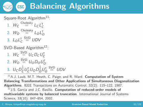
Balancing Algorithms
Square-Root Algorithm11:
1. WCCholesky
= LCLᵀC
2. WOCholesky
= LOLᵀO
3. LOLᵀC
SVD= UDV
SVD-Based Algorithm12:
1. WCSVD= UCDCU
ᵀC
2. WOSVD= UODOU
ᵀO
3. UCD12CU
ᵀCUOD
12OU
ᵀO
SVD= UDV
11A.J. Laub, M.T. Heath, C. Paige, and R. Ward. Computation of SystemBalancing Transformations and Other Applications of Simultaneous DiagonalizationAlgorithms. IEEE Transactions on Automatic Control, 32(2): 115–122, 1987.
12J.S. Garcia and J.C. Basilio. Computation of reduced-order models ofmultivariable systems by balanced truncation. International Journal of SystemsScience, 33(10): 847–854, 2002.
C. Himpe, [email protected] Gramian-Based Model Reduction 62/128

Approximate Balancing
EVD-Based Balancing13:
1. WXEVD= UDV
SVD-Based Approximate Balancing7:
1. WXSVD= UDV
Direct Truncation: V ← Uᵀ
13R.W. Aldhaheri. Model order reduction via real Schur-form decomposition.International Journal of Control, 53(3): 709–716, 1991.
C. Himpe, [email protected] Gramian-Based Model Reduction 63/128

Truncation
Truncation Operator:
S =
(1n
0
)∈ RN×n
Let U and V be a balancing transformation.
Then: U1 := U ◦ S , V1 := Sᵀ ◦ V .
This masks out the least important (balanced) states.
Zero vector field components are constant,
hence, can be discarded.
C. Himpe, [email protected] Gramian-Based Model Reduction 64/128

Practical Computation
Computing Lyapunov and Sylvester equations:
Bartels-Stewart14
Sign function15
Alternating Direction Implicit Iteration (ADI)16
...
14R. Bartels and G. Stewart. Solution of the Matrix Equation AX + XB = C.Communication of the ACM, 15(9): 820–826, 1972.
15U. Baur and P. Benner. Cross-Gramian Based Model Reduction for Data-SparseSystems. Electronic Transactions on Numerical Analysis, 31: 256–270, 2008.
16J. Saak, P. Benner and P. Kurschner. A Goal-Oriented Dual LRCF-ADI forBalanced Truncation. IFAC Proceedings Volumes, 45(2): 752–757, 2012.
C. Himpe, [email protected] Gramian-Based Model Reduction 65/128

Stability Preservation
Balanced truncation is stability preserving17.
Approximate balancing generally not, but often is.
Non-symmetric cross Gramian preserves stability8.
17L. Pernebo and L. Silverman. Model Reduction via Balanced State SpaceRepresentations. IEEE Transactions on Automatic Control, 27(2): 382–387, 1982.
C. Himpe, [email protected] Gramian-Based Model Reduction 66/128

Error BoundsH∞ Error Bound18,19:
‖G − Gr‖H∞ ≤ 2N∑
i=n+1
σi(H)
L1 Error Bound20:
‖g − gr‖L1 ≤ 4(N + n)N∑
i=n+1
σi(H)
18D.F. Enns. Model Reduction with Balanced Realizations: An Error Bound and aFrequency Weighted Generalization. In IEEE Conference on Decision and Control, vol.23: 127–132, 1984.
19K. Glover. All optimal Hankel-norm approximations of linear multivariablesystems and their L∞-error bounds. International Journal of Control, 39(6):1115–1193, 1984.
20J. Lam and B.D.O Anderson. L1 Impulse Response Error Bound for BalancedTruncation. System & Control Letters, 18(2): 129–137, 1992.
C. Himpe, [email protected] Gramian-Based Model Reduction 67/128

Error Indicator
H2 Error Indicator7:
‖G − Gr‖H2 ≈√
tr(C2W22B2)
H2 norm: ‖G‖H2 =√
tr(CWCC ᵀ) =√
tr(BᵀWOB)
Balanced system matrices: A, B , C
Balanced Gramian: W =
σ1(H). . .
σN(H)
C. Himpe, [email protected] Gramian-Based Model Reduction 68/128

Second-Order Systems
Second-Order System:
Mq(t) + Gq(t) + Kq(t) = BVu(t)
y(t) = CPq(t) + CV q(t)
First-Order Representation:(xP(t)xV (t)
)=
(0 1
−M−1K −M−1G
)(xP(t)xV (t)
)+
(0
M−1BV
)u(t)
y(t) =(CP CV
)(xP(t)xV (t)
)
C. Himpe, [email protected] Gramian-Based Model Reduction 69/128

Second-Order Balanced Truncation
Second-Order System Gramians21:
WC =
(WC ,P WC ,12
WC ,21 WC ,V
), WO =
(WO,P WO,12
WO,21 WO,V
), WX =
(WX ,P WX ,12
WX ,21 WX ,V
)
Position and velocity projections: UP,1, VP,1, UV ,1, VV ,1
Generally not stability preserving.
Preserves second-order structure.
21T. Reis and T. Stykel. Balanced truncation model reduction of second-ordersystems. Mathematical and Computer Modelling of Dynamical Systems: Methods,Tools and Applications in Engineering and Related Sciences, 14(5): 391–406, 2008.
C. Himpe, [email protected] Gramian-Based Model Reduction 70/128
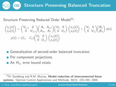
Structure Preserving Balanced Truncation
Structure Preserving Reduced Order Model22:(xα(t)xβ(t)
)=
(Vα,1 0
0 Vβ,1
)(Aα AαβAβα Aβ
)(Uα 00 Uβ
)(xα(t)xβ(t)
)+
(Vα 00 Vβ
)(BαBβ
)u(t)
y(t) =(Cα Cβ
)(Uα 00 Uβ
)(xα(t)xβ(t)
)
Generalization of second-order balanced truncation.
Per component projections.
An H∞ error bound exists.
22H. Sandberg and R.M. Murray. Model reduction of interconnected linearsystems. Optimal Control Applications and Methods, 30(3): 225–245, 2009.
C. Himpe, [email protected] Gramian-Based Model Reduction 71/128

Structured Reduction
General Structured Model:(xα(t)xβ(t)
)=
(fα(xα(t), xβ(t), u(t), θ)fβ(xα(t), xβ(t), u(t), θ)
)y(t) = g(xα(t), xβ(t), u(t), θ)
Structured Reduced Order Model:(xα,r(t)xβ,r(t)
)=
(Vα,1 fα(Uα,1xα,r(t), Uβ,1xβ,r(t), u(t), θ)Vβ,1 fβ(Uα,1xα,r(t), Uβ,1xβ,r(t), u(t), θ)
)yr(t) = g(Uα,1xα,r(t),Uβ,1xβ,r(t), u(t), θ)
C. Himpe, [email protected] Gramian-Based Model Reduction 72/128

Singular Perturbation
Singular Perturbation Reduced Order System Matrices23:
Ar := A11 − A12A−122 A21
Br := B1 − A12A−122 B2
Cr := C1 − C2A−122 A21
Balanced Truncation better for s →∞Singular Perturbation better for s → 0
Instead of truncating (BT), keep at steady state (SP).
Practically, a Schur complement.
H∞ Error bound and stability preservation hold.
23G. Obinata and B.D.O. Anderson. Model Reduction for Control System Design.Communications and Control Engineering. Springer, 2001.
C. Himpe, [email protected] Gramian-Based Model Reduction 73/128
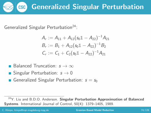
Generalized Singular Perturbation
Generalized Singular Perturbation24:
Ar := A11 + A12(s01− A22)−1A21
Br := B1 + A12(s01− A22)−1B2
Cr := C1 + C2(s01− A22)−1A21
Balanced Truncation: s →∞Singular Perturbation: s → 0
Generalized Singular Perturbation: s = s0
24Y. Liu and B.D.O. Anderson. Singular Perturbation Approximation of BalancedSystems. International Journal of Control, 50(4): 1379–1405, 1989.
C. Himpe, [email protected] Gramian-Based Model Reduction 74/128

Balanced Gains
Norm identity:
‖G‖H2 = tr(
∫ ∞0
yᵀ(t)y(t) dt) = tr(C ᵀCWC ) = tr(BBᵀWO)
Balanced system: A, B , C
B =(b1 . . . bM
), C =
(cᵀ1 . . . cᵀQ
)ᵀIn balanced form: ‖G‖H2 =
∑Ni=1 c
2i σi(H) =
∑Ni=1 b
2i σi(H)
Balanced gains25: di := c2i σi(H) = b2
i σi(H)
BG sometimes better, sometimes worse than BT.
25A. Davidson. Balanced Systems and Model Reduction. Electronics Letters,22(10): 531–532, 1986.
C. Himpe, [email protected] Gramian-Based Model Reduction 75/128

Part III: Nonlinear Gramian-Based Model Reduction
1. Empirical Gramians
2. Empirical Balanced Truncation
3. The Averaging Principle
4. Gramian-Based Parameter Identification
5. Combined State and Parameter Reduction
C. Himpe, [email protected] Gramian-Based Model Reduction 76/128

Linearized Balanced Truncation
Linearization:
A` :=∂
∂xf (x , u), B` :=
∂
∂uf (x , u), C` :=
∂
∂xg(x , u)
Linearize at steady state.
Compute balanced truncation projections.
Use these on nonlinear model26.
26X. Ma and J.A. De Abreu-Garcia. On the Computation of Reduced Order Modelsof Nonlinear Systems using Balancing Technique. In Proceedings of the 27th IEEEConference on Decision and Control, vol 2: 1165–1166, 1988.
C. Himpe, [email protected] Gramian-Based Model Reduction 77/128

Nonlinear Balancing
Controllability energy and observability energy:
LC := minu∈L2
1
2
∫ 0
−∞‖u(t)‖2 dt =
1
2xᵀ0W
−1C x0
LO :=1
2
∫ ∞0‖y(t)‖2 dt =
1
2xᵀ0WOx0
Control-affine system: x(t) = f (x(t)) + h(x(t))u(t), y(t) = g(x(t))
Nonlinear controllability Gramian: ∂LC∂x f (x) + 1
2∂LC∂x h(x)hᵀ(x)∂LC∂x = 0
Nonlinear observability Gramian: ∂LO∂x f (x) + 1
2gᵀ(x)g(x) = 0
Nonlinear balancing truncation27
Numerically infeasible for large systems.
27J.M.A. Scherpen. Balancing for nonlinear systems. Systems & Control Letters,21(2): 143–153, 1993.
C. Himpe, [email protected] Gramian-Based Model Reduction 78/128

Empirical Gramians
System Gramians:
WC =
∫ ∞0
(eAt B)(eAt B)ᵀ dt
WO =
∫ ∞0
(eAᵀt C )(eA
ᵀt C ᵀ)ᵀ dt
WX =
∫ ∞0
(eAt B)(eAᵀt C ᵀ)ᵀ dt
Integrands are impulse responses.
Data-driven computation.
Applicable for nonlinear systems.
C. Himpe, [email protected] Gramian-Based Model Reduction 79/128

Empirical Gramian Principles
(Auto-)Correlation:
W :=
∫ ∞0
(x(t)− x)(x(t)− x)ᵀ dt
Temporal Mean:
x = limT →∞
∫ ∞0
x(t) dt
Averaging:
W =1
N
N∑i=1
Wi
C. Himpe, [email protected] Gramian-Based Model Reduction 80/128

Operating Region
Input Perturbations:
Direction: Eu = {ei ∈ RM ; ‖ei‖ = 1; 〈ei , ej 6=i〉 = 0; i , j = 1, ...,M}Rotation: Ru = {Si ∈ RM×M ; Sᵀ
i Si = 1M ; i = 1, ..., s}Scale: Qu = {ci ∈ R; ci > 0; i = 1, ..., q}
Initial State Perturbations:
Direction: Ex = {fi ∈ RN ; ‖fi‖ = 1; 〈fi , fj 6=i〉 = 0; i , j = 1, ...,N}Rotation: Rx = {Ti ∈ RN×N ;T ᵀ
i Ti = 1N ; i = 1, ..., t}Scale: Qx = {di ∈ R; di > 0; i = 1, ..., r}
C. Himpe, [email protected] Gramian-Based Model Reduction 81/128

Empirical Controllability Gramian
Empirical Controllability Gramian28:
WC =1
|Qu||Ru|
|Qu |∑h=1
|Ru |∑i=1
M∑j=1
1
c2h
∫ ∞0
Ψhij(t) dt ∈ RN×N
Ψhij(t) = (xhij(t)− xhij)(xhij(t)− xhij)ᵀ ∈ RN×N
Non-trivial sets: Eu, Ru, Qu
xhij(t) is trajectory for input: uhij(t) = chSiejδ(t)
Temporal mean state: xhij
28S. Lall, J.E. Marsden, and S. Glavaski. Empirical Model Reduction of ControlledNonlinear Systems. In Proceedings of the 14th IFAC Congress, vol. F: 473–478, 1999.
C. Himpe, [email protected] Gramian-Based Model Reduction 82/128

Empirical Controllability Covariance Matrix
Empirical Controllability Covariance Matrix29:
WC =1
|Qu||Ru|
|Qu |∑h=1
|Ru |∑i=1
M∑j=1
1
c2h
∫ ∞0
Ψhij(t) dt ∈ RN×N
Ψhij(t) = (xhij(t)− xhij)(xhij(t)− xhij)ᵀ ∈ RN×N
Non-trivial sets: Eu, Ru, Qu
xhij(t) is trajectory for input: uhij(t) = chSiej � u(t) + u
Steady-state: x
Steady-state input: u29J. Hahn and T.F. Edgar. Balancing Approach to Minimal Realization and Model
Reduction of Stable Nonlinear Systems. Industrial & Engineering Chemistry Research,41(9): 2204–2212, 2002.
C. Himpe, [email protected] Gramian-Based Model Reduction 83/128

Empirical Observability Gramian
Empirical Observability Gramian25:
WO =1
|Qx ||Rx |
|Qx |∑k=1
|Rx |∑l=1
1
d2k
∫ ∞0
TlΨkl(t)T ᵀ
l dt ∈ RN×N
Ψklab(t) = (y kla(t)− y kla)ᵀ(y klb(t)− y klb) ∈ R
Non-trivial sets: Ex , Rx , Qx
y kla(t) is output trajectory for initial state: xkla0 = dkTl fa
Temporal mean output: y kla
C. Himpe, [email protected] Gramian-Based Model Reduction 84/128

Empirical Observability Covariance Matrix
Empirical Observability Covariance Matrix26:
WO =1
|Qx ||Rx |
|Qx |∑k=1
|Rx |∑l=1
1
d2k
∫ ∞0
TlΨkl(t)T ᵀ
l dt ∈ RN×N
Ψklab(t) = (y kla(t)− y kla)ᵀ(y klb(t)− y klb) ∈ R
Non-trivial sets: Ex , Rx , Qx
y kla(t) is output trajectory for initial state: xkla0 = dkTl fa + x
Steady-state: x
Steady state output: y
C. Himpe, [email protected] Gramian-Based Model Reduction 85/128

Empirical Linear Cross Gramian
Empirical Linear Cross Gramian30:
WY =1
|Qu||Ru|
|Qu |∑h=1
|Ru |∑i=1
M∑j=1
1
c2h
∫ ∞0
Ψhij(t) dt ∈ RN×N
Ψhij(t) = (xhij(t)− xhij)(zhij(t)− zhij)ᵀ ∈ RN×N
Non-trivial sets: Eu, Ru, Qu
xhij is trajectory for input: uhij(t) = chSiejδ(t)
zhij is adjoint trajectory for input vhij(t) = chSiejδ(t)
Temporal mean: xhij
Adjoint temporal mean: zhij30U. Baur, P. Benner, B. Haasdonk, C. Himpe, I. Martini and M. Ohlberger.
Comparison of Methods for Parametric Model Order Reduction of Time-DependentProblems. In: Model Reduction and Approximation: Theory and Algorithms, Editors: P.Benner, A. Cohen, M. Ohlberger and K. Willcox, SIAM: 377–407, 2017.
C. Himpe, [email protected] Gramian-Based Model Reduction 86/128

Empirical Cross Gramian
Empirical Cross Gramian31:
WX =
|Qu |∑h=1
|Ru |∑i=1
M∑j=1
|Qx |∑k=1
|Rx |∑l=1
1
chdk
∫ ∞0
TlΨhijkl(t)T ᵀ
l dt ∈ RN×N
Ψhijklab (t) = f ᵀb T
ᵀl (xhij(t)− xhij)eᵀj S
ᵀi (y kla(t)− y kla) ∈ R
Non-trivial sets: Eu, Ex , Ru, Rx , Qu, Qx
xhij is trajectory for input: uhij(t) = chSiejδ(t)
y kla is output trajectory for initial state: xkla0 = dkTl faTemporal mean state: xhij
Temporal mean output: y kla
Efficient computation of empirical non-symmetric cross Gramian8.31C. Himpe and M. Ohlberger. Cross-Gramian Based Combined State and
Parameter Reduction for Large-Scale Control Systems. Mathematical Problems inEngineering, 2014:1–13, 2014.
C. Himpe, [email protected] Gramian-Based Model Reduction 87/128

Empirical Cross Covariance Matrix
Empirical Cross Covariance Matrix31:
WX =
|Qu |∑h=1
|Ru |∑i=1
M∑j=1
|Qx |∑k=1
|Rx |∑l=1
1
chdk
∫ ∞0
TlΨhijkl(t)T ᵀ
l dt ∈ RN×N
Ψhijklab (t) = f ᵀb T
ᵀl (xhij(t)− xhij)eᵀj S
ᵀi (y kla(t)− y kla) ∈ R
Non-trivial sets: Eu, Ex , Ru, Rx , Qu, Qx
xhij is trajectory for input uhij(t) = chSiej � u(t) + u
y kla is output trajectory for initial state xkla0 = dkTl fa + x
Steady-state: x
Steady-state input: u
Steady-state output: y
C. Himpe, [email protected] Gramian-Based Model Reduction 88/128
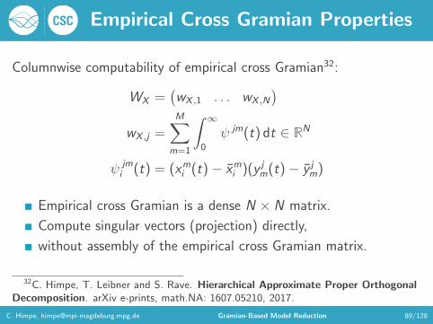
Empirical Cross Gramian Properties
Columnwise computability of empirical cross Gramian32:
WX =(wX ,1 . . . wX ,N
)wX ,j =
M∑m=1
∫ ∞0
ψ jm(t) dt ∈ RN
ψ jmi (t) = (xmi (t)− xmi )(y j
m(t)− y jm)
Empirical cross Gramian is a dense N × N matrix.
Compute singular vectors (projection) directly,
without assembly of the empirical cross Gramian matrix.
32C. Himpe, T. Leibner and S. Rave. Hierarchical Approximate Proper OrthogonalDecomposition. arXiv e-prints, math.NA: 1607.05210, 2017.
C. Himpe, [email protected] Gramian-Based Model Reduction 89/128

Nonlinear Error Indicators
Relative Information Content:
ε1 :=‖Hr‖∗‖H‖∗
=
∑ni=1 σi(H)∑Ni=1 σi(H)
Linear Error Indicators:
‖y − yr‖H∞ . 2∑N
i=n+1 σi(H)
‖y − yr‖H2 ≈√
tr(C`,2W22B`,2)
‖y − yr‖L1 . 4(N + n)∑N
i=n+1 σi(H)
C. Himpe, [email protected] Gramian-Based Model Reduction 90/128
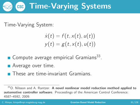
Time-Varying Systems
Time-Varying System:
x(t) = f (t, x(t), u(t))
y(t) = g(t, x(t), u(t))
Compute average empirical Gramians33.
Average over time.
These are time-invariant Gramians.
33O. Nilsson and A. Rantzer. A novel nonlinear model reduction method applied toautomotive controller software. Proceedings of the American Control Conference:4587–4592, 2009.
C. Himpe, [email protected] Gramian-Based Model Reduction 91/128

Inner Products and Kernels
Inner Product34:
Galerkin projections are not stability preserving.
Adapting the inner product can fix this.
For example: energy-stable inner products.
Kernel35:
Think of kernels as generalized inner products.
Kernel trick: Only evaluate inner product in nonlinear space.
Mapping back to the original space is more expensive.
34I. Kalashnikova, M.F. Barone, S. Arunajatesan, B.G. Van Bloemen Waanders.Contruction of energy-stable projection-based reduced order models. AppliedMathematics and Computation, 249: 569–596, 2014.
35J. Bouvrie and B. Hamzi. Kernel Methods for the Approximation of NonlinearSystems. SIAM Journal on Control and Optimization, 55(4): 2460–2492, 2017.
C. Himpe, [email protected] Gramian-Based Model Reduction 92/128

Parametric Systems
Linearly Parametric Linear System:
x(t) = Ax(t) + Bu(t) + Fθ = Ax(t) +(B F
)( u(t)uθ(t)
)Parametric Empirical Gramians30:
WC ,θ :=P∑i=1
WC (θi)
Parameter input: uθ(t) = θ
Observability is adjoint controllability: WO,θ :=∑
i WO(θi)
Parametric empirical cross Gramian: WX ,θ :=∑
i WX (θi)
C. Himpe, [email protected] Gramian-Based Model Reduction 93/128
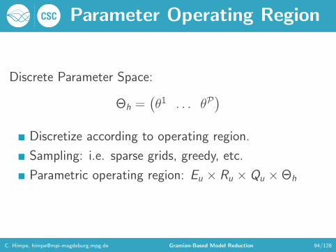
Parameter Operating Region
Discrete Parameter Space:
Θh =(θ1 . . . θP
)Discretize according to operating region.
Sampling: i.e. sparse grids, greedy, etc.
Parametric operating region: Eu × Ru × Qu ×Θh
C. Himpe, [email protected] Gramian-Based Model Reduction 94/128

Parameter Reduction
Parameter Covariance:
ωSVD= Π
σ1. . .
σP
Πᵀ
Use same machinery as for states.
Parameter Galerkin projections via SVD.
How to compute parameter covariances?
C. Himpe, [email protected] Gramian-Based Model Reduction 95/128

Controllability-Based Parameter Reduction
Linearly Parametric Linear System:
x(t) = Ax(t) + Bu(t) + Fθ = Ax(t) + Bu(t) +P∑i=1
Fiθi
→ WC = WC ,0 +P∑i=1
WC ,i
WC ,0 =
∫ ∞0
eAt BBᵀ eAᵀt dt, WC ,i =
∫ ∞0
eAt FiFᵀi eA
ᵀt dt
Empirical Sensitivity Gramian:
WS :=
tr(WC ,1). . .
tr(WC ,P)
C. Himpe, [email protected] Gramian-Based Model Reduction 96/128

Observability-Based Parameter Reduction
Augmented System:(x(t)
θ(t)
)=
(f (x(t), u(t), θ(t))
θ0
)y(t) = g(x(t), u(t), θ(t))
Augmented Observability Gramian:
W O =
(WO WM
W ᵀM WP
)Empirical Identifiability Gramian:
WI := WP −W ᵀMW−1
O WM ≈ WP
Related to Fischer information matrix.
C. Himpe, [email protected] Gramian-Based Model Reduction 97/128

Cross-Gramian-Based Parameter Reduction
Empirical Joint Gramian31:
WJ := W X =
(WX WM
Wm WP
)=
(WX WM
0 0
)Empirical Cross-Identifiability Gramian31:
WI = −1
2W ᵀ
M(WX + W ᵀX )−1WM
Lower blocks are zero as parameters are uncontrollable.
WI encodes observability of parameters.
Schur complement can be approximated efficiently.
C. Himpe, [email protected] Gramian-Based Model Reduction 98/128

Combined State and Parameter Reduction
Combined Reductions:
State-space reduction via empirical Gramians
Parameter-space reduction via empirical Gramians
Compound computation
Abbreviations:
BT = Balanced Truncation
DT = Direct Truncation
C. Himpe, [email protected] Gramian-Based Model Reduction 99/128

Controllability-Based Combined Reduction
1. Compute WS (includes WC )
2. Compute WO
3. State-Space Reduction: BT(WC , WO)
4. Parameter-Space Reduction: DT(WS)
C. Himpe, [email protected] Gramian-Based Model Reduction 100/128

Observability-Based Combined Reduction
1. Compute WC
2. Compute WI (includes WO)
3. State-Space Reduction: BT(WC , WO)
4. Parameter-Space Reduction: DT(WI )
C. Himpe, [email protected] Gramian-Based Model Reduction 101/128

Cross-Gramian-Based Combined Reduction
1. Compute WJ (includes WX , WI )
2. State-Space Reduction: DT(WX )
3. Parameter-Space Reduction: DT(WI )
C. Himpe, [email protected] Gramian-Based Model Reduction 102/128
About Empirical-Gramian-Based Combined Reduction
Works for high-dimensional parameter-spaces!
Combined computation of state and parameter Gramians.
Preferably for control-affine systems.
Definition of operating region (around a steady state) paramount.
Simulation trajectory quality determines reduced model quality.
C. Himpe, [email protected] Gramian-Based Model Reduction 103/128
Part IIII: Combined Reduction Examples
1. Linear Benchmark: Inverse Lyapunov Procedure
2. Nonlinear Benchmark: RC Ladder
3. Hyperbolic Network Model
4. EEG Dynamic Causal Model
5. fMRI Dynamic Causal Model
C. Himpe, [email protected] Gramian-Based Model Reduction 104/128

emgr - EMpirical GRamian Framework (Version: 5.2)
Empirical Gramians:
Empirical Controllability GramianEmpirical Observability GramianEmpirical Linear Cross GramianEmpirical Cross GramianEmpirical Sensitivity GramianEmpirical Identifiability GramianEmpirical Joint Gramian
Features:
Interfaces for: Solver, inner product kernels & distributed memoryNon-Symmetric option for all cross GramiansFunctional designCompatible with OCTAVE and MATLABVectorized and parallelizableOpen-source licensed
More info: http://gramian.de
C. Himpe, [email protected] Gramian-Based Model Reduction 105/128

Inverse Lyapunov Procedure
Linear-Linear System:
x(t) = Ax(t) + Bu(t) + Fθ
y(t) = Cx(t)
Inverse Lyapunov Procedure36
1. Sample eigenvalues of WC and WO .
2. Sample eigenvectors of WC and WO .
3. Normalize B and C .
4. Compute A via Lyapunov equation.
5. Unbalance system.
36S.C. Smith and J. Fisher. On generating random systems: a gramian approach.In Proceedings of the American Control Conference, vol. 3: 2743–2748, 2003.
C. Himpe, [email protected] Gramian-Based Model Reduction 106/128

Relative Combined Reduction L2 ⊗ L2 Error
Controllability-based, observability-based, and cross-Gramian-based combined reduction.
C. Himpe, [email protected] Gramian-Based Model Reduction 107/128

Nonlinear RC Ladder
SISO Nonlinear RC Cascade37:
x(t) = f (x(t)) + A(θ)x(t) + Bu(t)
y(t) = Cx(t)
Linear Parametrization.
Dimensionality: P = N
Good-natured nonlinearity.
37Y. Chen. Model Order Reduction for Nonlinear Systems. Master’s thesis,Massachusetts Institute of Technology, 1999.
C. Himpe, [email protected] Gramian-Based Model Reduction 108/128

Relative Combined Reduction L2 ⊗ L2 Error
2040
6080
100
2040
6080
100
10-16
10-14
10-12
10-10
10-8
10-6
10-4
10-2
100
Parame
ter
State
C. Himpe, [email protected] Gramian-Based Model Reduction 109/128

Hyperbolic Network Model
Hyperbolic Network Model38:
x(t) = A tanh(K (θ)x(t)) + Bu(t)
y(t) = Cx(t)
Parametrization: Kij(θ) =
{θi i = j
0 i 6= j
Dimensionality: P = N
Sigmoid nonlinearity.
38Y. Quan, H. Zhang, and L. Cai. Modeling and Control Based on a New NeuralNetwork Model. In Proceedings of the American Control Conference, vol. 3:1928–1929, 2001.
C. Himpe, [email protected] Gramian-Based Model Reduction 110/128

Relative Combined Reduction L2 ⊗ L2 Error
2040
6080
100
2040
6080
100
10-16
10-14
10-12
10-10
10-8
10-6
10-4
10-2
100
Parame
ter
State
C. Himpe, [email protected] Gramian-Based Model Reduction 111/128

Dynamic Causal Modelling
Practically:
Inference of brain region connectivity
from functional imaging data (EEG, fMRI).
Combined reduction for inverse problem.
Mathematically:
Two component model
Network dynamics sub-model
Measurement sub-model
C. Himpe, [email protected] Gramian-Based Model Reduction 112/128

EEG Dynamic Causal Model
EEG & MEG Dynamic Causal Model39:(v(t)x(t)
)=
(0 1−T −T 2
)(v(t)x(t)
)+
(0
A(θ)
)ς(Kx(t)) +
(0B
)u(t)
y(t) = Lx(t)
Parametrization: Aij(θ) = θi∗K+j
Dimensionality: P = N2
100
Second-order system with sigmoid nonlinearity.
39O. David, S.J. Kiebel, L.M. Harrison, J. Mattout, J.M. Kilner, and K.J. Friston.Dynamic causal modeling of evoked responses in EEG and MEG. NeuroImage, 4:1255–1272, 2006.
C. Himpe, [email protected] Gramian-Based Model Reduction 113/128
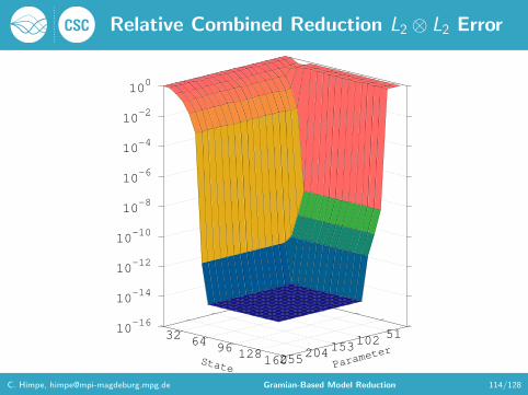
Relative Combined Reduction L2 ⊗ L2 Error
51102
153204
255
3264
96128
160
10-16
10-14
10-12
10-10
10-8
10-6
10-4
10-2
100
Parame
ter
State
C. Himpe, [email protected] Gramian-Based Model Reduction 114/128

fMRI Dynamic Causal Model
fMRI Dynamic Causal Model40:
x(t) = A(θ)x(t) + Bu(t)
s(t) = x(t)− κs(t)− γ(f (t)− 1)
f (t) = s(t)
v(t) =1
τ(f (t)− v(t)
1α )
q(t) =1
τ(
1
ρf (t)(1− ((1− ρ))
1f (t) )− v(t)
1α−1q(t))
y(t) = V0(k1(1− q(t)) + k2(1− v(t)))
Parametrization: Aij(θ) = θi∗K+j
Dimensionality: P = N2
25
Highly nonlinear system.40K.J. Friston, L.M. Harrison, and W. Penny. Dynamic causal modelling.
NeuroImage, 19(4): 1273–1302, 2003.
C. Himpe, [email protected] Gramian-Based Model Reduction 115/128

Relative Combined Reduction L2 ⊗ L2 Error
51102
153204
255
1632
4864
80
10-16
10-14
10-12
10-10
10-8
10-6
10-4
10-2
100
Parame
ter
State
C. Himpe, [email protected] Gramian-Based Model Reduction 116/128
Part V: Other Uses for System Gramians
1. Parameter Hessians
2. Decentralized Control
3. Nonlinearity Quantification
4. Sensitivity Analysis
5. System Indices
C. Himpe, [email protected] Gramian-Based Model Reduction 117/128

Newton-Type Optimization
Optimization problem subject to control system:
θ = arg minθ∈Θ ‖yd − y(θ)‖22
s.t.:
x(t) = f (x(t), u(t), θ)
y(t) = g(x(t), u(t), θ)
Newton-Type Algorithm:
Derivative-based optimization.
Requires Hessian or an approximation.
Identifiability Gramian can be used as Hessian41 (approximation).
41C. Lieberman and B. Van Bloemen Waanders. Hessian-Based Model ReductionApproach to Solving Large-Scale Source Inversion Problems. In CSRI SummerProceedings: 37–48, 2007.
C. Himpe, [email protected] Gramian-Based Model Reduction 118/128

Decentralized Control
MIMO System:
x(t) = f (x(t), u(t))
y(t) = g(x(t), u(t))
Which SISO subsystems are dominant?
Participation matrix: Pij =tr(Wij )
2
tr(W 2ij )
, i = 1 . . .M , j = 1 . . .Q
Decentralization: Max elements per row or column of P .
C. Himpe, [email protected] Gramian-Based Model Reduction 119/128

Nonlinearity Quantification
Nonlinear System:
x(t) = f (x(t), u(t))
y(t) = g(x(t), u(t))
Gramian-based nonlinearity indices42:
Input nonlinearity:∑N
i=1
∑Nj=1 |WC − WC |ij/ tr(WC )
State nonlinearity:∑N
i=1
∑Nj=1 |WX − WX |ij/ tr(WX )
Output nonlinearity:∑N
i=1
∑Nj=1 |WO − WO |ij/ tr(WO)
42J. Hahn and T.F. Edgar. A Gramian Based Approach to NonlinearityQuantification and Model Classification. Industrial & Engineering Chemistry Research,40(24): 5724–5731, 2001.
C. Himpe, [email protected] Gramian-Based Model Reduction 120/128

System Gain
System gain aka DC gain aka L2 gain:
S := tr(G (0)) = tr(CA−1B)
System gain via cross Gramian: S(G ) = −12 tr(WX )
Frequency response for s = 0.
Model reduction based on first order moments (HEV).
C. Himpe, [email protected] Gramian-Based Model Reduction 121/128

Sensitivity Analysis
Input-Parametric System:
x(t) = f (x(t), uθ(t))
y(t) = g(x(t), uθ(t))
Treat parameters as inputs: uθ(t) = θ.
Parameter sensitivity: S(θ) := y−yθ−θ = S(G (0)).
Gain computation via empirical cross Gramian43.
43S. Streif, R. Findeisen, and E. Bullinger. Relating Cross Gramians and SensitivityAnalysis in Systems Biology. Theory of Networks and Systems, 10.4: 437–442, 2006.
C. Himpe, [email protected] Gramian-Based Model Reduction 122/128

Cauchy Index
Cauchy-Index via cross Gramian44:
C =N∑i=1
sign(λi(WX ))
C := p+ − p−
p+ are transfer function poles w. positive residue
p− are transfer function poles w. negative residue
44K.V. Fernando and H. Nicholson. On the Cauchy Index of Linear Systems. IEEETransactions on Automatic Control , 28(2):222–224, 1983.
C. Himpe, [email protected] Gramian-Based Model Reduction 123/128

Information Entropy
Information entropy via cross Gramian:
I :=N
2ln(2π e) +
1
2ln(det(WX ))
Minimizing information loss45.
Meaning minimzing steady-state information entropy.
Basically Kullback-Leibler divergence minimization.
45J. Fu, C. Zhong, Y. Ding, J. Zhou and C. Zhong. An information theoreticapproach to model reduction based on frequency-domain Cross-Gramianinformation. In 8th World Congress on Intelligent Control and Automation: 3679–3683,2010
C. Himpe, [email protected] Gramian-Based Model Reduction 124/128

Summary
Linear Gramian-Based Model Reduction
Balanced TruncationSingular PerturbationApproximate BalancingDirect Truncation
Nonlinear Gramian-Based Model Reduction
Empirical Balanced TruncationEmpirical Direct Truncation
Parameter Identification and Parameter Reduction
Gramian-Based Combined State and Parameter Reduction
C. Himpe, [email protected] Gramian-Based Model Reduction 125/128

Takeaway Messages
Balanced truncation is the gold standard.
Use algebraic methods for plain linear systems.
Empirical Gramians are not always the best,
but are almost always computable.
Empirical Gramians are all about averaging.
The more you know about the operating region the better.
The quality of simulations determines the quality of the ROM.
C. Himpe, [email protected] Gramian-Based Model Reduction 126/128

Not Covered
... but also interesting:
Descriptor Systems
Unstable Systems
Bilinear Systems
Quadratic Systems
Switched Systems
Active Subspaces
...
C. Himpe, [email protected] Gramian-Based Model Reduction 127/128

That’s All Folks
Slides: http://himpe.science/talks/himpe17-issac.pdf
Lab Session: 2017–09–12, 1400–1730
Questions?
http://himpe.science
Acknowledgment:Supported by the German Federal Ministry for Economic Affairs andEnergy, in the joint project: “MathEnergy – Mathematical KeyTechnologies for Evolving Energy Grids”, sub-project: Model OrderReduction (Grant number: 0324019B).
C. Himpe, [email protected] Gramian-Based Model Reduction 128/128