Contents lists available at ScienceDirect

Computers and Geotechnics

journal homepage: www.elsevier.com/locate/compgeo

Research Paper

Granular viscosity from plastic yield surfaces: The role of the deformationtype in granular flowsM. Rautera,b,⁎, T. Barkerc,d, W. Felline

aNorwegian Geotechnical Institute, Department of Natural Hazards, Oslo, NorwaybUniversity of Oslo, Department of Mathematics, Oslo, NorwaycUniversity of Manchester, Applied Mathematics, Manchester, United KingdomdUniversity of Edinburgh, School of GeoSciences, Edinburgh, United KingdomeUniversity of Innsbruck, Institute of Infrastructure, Division of Geotechnical and Tunnel Engineering, Innsbruck, Austria

A R T I C L E I N F O

Keywords:Granular flowsRheologyYield surfacePlasticityCFD

A B S T R A C T

Numerical simulations of granular flows with Navier–Stokes type models emerged in the last decade, challengingthe well established depth-averaged models. The structure of these equations allows for extension to generalrheologies based on complex and realistic constitutive models. Substantial effort has been put into describing theeffect of the shear rate, i.e. the magnitude of the velocity gradient, on the shear stress. Here we analyse the effectof the deformation type. We apply the theories of Mohr–Coulomb and Matsuoka–Nakai to calculate the stressesunder different deformation types and compare results to the theory of Drucker–Prager, which is formulatedindependently of the deformation type. This model is particularly relevant because it is the basis for manygranular rheologies, such as the µ I( )–rheology. All models have been implemented into the open-source toolkitOpenFOAM® for a practical application. We found that, within the context of these models, the deformation typehas a large influence on the stress. However, for the geometries considered here, these differences are limited tospecific zones which have little influence on the landslide kinematics. Finally we are able to give indicators onwhen the deformation type should be considered in modelling of landslides and when it can be neglected.

1. Introduction

Dense granular flows are substantial parts of many natural hazards,such as avalanches, landslides, debris flows and lahars. A constitutivedescription of granular materials is important for a deeper under-standing and improved prediction of these processes.

The first models for granular materials stem from geotechnics andapplications in the soil mechanics community, with the earliest ex-amples of a mathematical description being in the 19th century, whenCharles-Augustin de Coulomb formulated his famous friction law (seee.g. [1]), based on the rules found earlier by Guillaume Amontons (seee.g. [2]). It relates normal stress n and shear stress between twosolids and defines the friction angle as

=tan( ) .n (1)

This relation is limited to well defined sliding planes and not generallyapplicable to three-dimensional situations. Christian Otto Mohr gen-eralized Coulomb’s law by determining the decisive shear plane in afailing solid with arbitrary stress state. The resulting formulation is

known as the Mohr–Coulomb (MC) failure criterion [3]. The Mohr–-Coulomb failure criterion describes the failure of brittle materials, suchas concrete and granular material with good accuracy. In fact, it hasbeen successfully applied to a wide range of problems, especially withinelasto-plastic frameworks [4]. Various extensions have been applied tothe original idea, introducing strain hardening and softening or so-called caps, limiting the admissible pressure [5]. Matsuoka and Nakai[6] proposed a smoother version of the Mohr–Coulomb criterion, theMatsuoka–Nakai (MN) failure criterion. It has gained a lot of popu-larity, as it improved numerical stability as well as physical accuracy.All developments were merged into modern constitutive models forquasi-static granular materials, such as the hardening-soil-model [5],Severn-Trent-sand [7], SaniSand [8], Hypoplasticity [9,10] or Barodesy[11–13].

All of the above models assume quasi-static conditions and describethe stresses at failure. The respective extension to dynamic cases hasbeen of interest for a long time. Schaeffer [14] was the first to combinethe two-dimensional Navier–Stokes Equations, with the quasi-staticMohr–Coulomb failure criterion. His work assumed that the

https://doi.org/10.1016/j.compgeo.2020.103492Received 6 November 2019; Received in revised form 20 January 2020; Accepted 11 February 2020

⁎ Corresponding author at: Norwegian Geotechnical Institute, N-0855 Oslo, Norway.E-mail addresses: matthias.rauter@ngi.no (M. Rauter), thomas.barker@ed.ac.uk (T. Barker), wolfgang.fellin@uibk.ac.at (W. Fellin).

Computers and Geotechnics 122 (2020) 103492

0266-352X/ © 2020 The Authors. Published by Elsevier Ltd. This is an open access article under the CC BY license (http://creativecommons.org/licenses/BY/4.0/).

T

Mohr–Coulomb failure stress is valid beyond failure and at any strainrate, an assumption which is consistent with ideal plasticity [4], wherefailure criterion and yield criterion are coinciding. In this sense we willuse henceforth the term yield criterion when computing the stress in aflowing material. Schaeffer’s theory matches Mohr–Coulomb only forplane strain (i.e. two dimensional deformations) and incompressibleflows, i.e. isochoric shear. Although he found some problematic in-stabilities, his work was highly influential in the granular flow com-munity and his approach was applied for both, plane strain and fullythree-dimensional granular flows, first and foremost in chemical en-gineering [15,16].

Early models assumed that the magnitude of the stress tensor re-mains constant after failure and independent of the shear rate. Thisassumption fails to describe various phenomena from physical experi-ments, e.g. steady flows on inclined planes or roll waves [17–20] and alarge amount of research has been attributed to describe the respectivecorrelations. Most notable are the early works of Bagnold [21,22] andVoellmy [23], both combining Coulomb’s friction law and an additionaldynamic term. More recent developments have been achieved withkinetic theory [24,25] and with the so-called µ I( )–rheology, relatingthe dimensionless friction coefficient =µ sin( ) to the dimensionlessinertial number I [18].

The first generally applicable µ I( )–rheology was introduced by Jopet al. [26], basically following the approach of Schaeffer [14] but with ashear rate dependent yield criterion. The instabilities found bySchaeffer [14] are partially present in the model of Jop et al. [26] andaddressed, among others, by Barker et al. [27,28].

Although the success of respective models is impressive, we have tocontemplate that Schaeffer’s approach is limited to plane, in-compressible deformation, i.e. isochoric shear. If his relation is used forarbitrary three-dimensional deformations, one gets what is commonlyknown as the Drucker–Prager (DP) yield criterion in solid mechanics[29]. The differences between Mohr–Coulomb and Drucker–Prager arewell known [30] and may be rather large, depending on the induceddeformation [31,32]. This yields, for example, remarkable errors inearth pressure calculations [33]. Furthermore, it has been revealed thatthe Mohr–Coulomb yield criterion is fulfilled in discrete element si-mulations to a much better degree than the Drucker–Prager yield cri-terion [34].

These circumstances lead to a big gap between Mohr–Coulombmodels, and the recent success of the µ I( )–rheology. This gap is whatwe aim to close with this work. We will extend the approach ofSchaeffer [14] and Jop et al. [26] to different yield criteria. This allowsus to implement constitutive models based on Mohr–Coulomb andMatsuoka–Nakai alongside the classic relation of Schaeffer [14] (i.e.Drucker–Prager) into the CFD-toolkit OpenFOAM® [35]. We are com-paring the three relations by inducing three-dimensional deformationsin granular flow simulations. We neglect the shear rate dependence ofstresses in this work to focus solely on the effect of the yield criterion.However, the µ I( )-scaling is perfectly compatible with all of the pre-sented yield criteria and can be easily reintroduced. To keep compu-tational demand to an acceptable level, we run axisymmetric cases,some of which have been validated with physical experiments [36]. Weare able to draw some conclusions and determine the circumstances forwhich the widely used Drucker–Prager relation differs from the tradi-tional Mohr–Coulomb relation.

2. Method

The incompressible Navier–Stokes Equations are given as

=u· 0, (2)

+ = + = +t

pu u u T g D g( ) ·( ) · ·(2 ) , (3)

with velocity u, density , stress tensor = pT T Idev , strain rate

tensor1 D, pressure =p T1/3tr( ) and gravitational acceleration g. Inthe following, we will assume that pore-pressure is negligibly small andhence that the pressure p is equal to the effective pressure p .

In order to combine granular rheologies with the Navier–StokesEquations, it is required to calculate the deviatoric stress tensor Tdev interms of the known strain rate tensor,

= = +D u u usym( ) 12

( ( ) ),T(4)

and the dynamic viscosity2 , or equivalently the kinematic viscosity= / (note the first term on the right-hand side of Eq. (3)). Therefore,

without substantial modification of the underlying equations, all con-stitutive modelling is reduced to the scalar viscosity. This introducessome severe limitations, namely alignment between stress and strainrate tensor, which we will illuminate below. The hydrostatic part of thestress tensor, p I can not be established with a constitutive relation inincompressible flow models (as =Dtr( ) 0) and is therefore calculatedfrom the constraint of the continuity Eq. (2) with e.g. the PISO algo-rithm [37].

2.1. A tensorial description of deformation and stress

The set of all stress tensors, at which yielding occurs forms a surfacein stress space, which we define as the yield surface (see Fig. 4). Ad-missible stress tensors of static material are located within the yieldsurface and stress tensors do not exist outside the yield surface [4].Vice-versa, a yield surface, in addition with the so called flow rule, issufficient to describe a perfectly plastic material. As we will show later,the flow rule is required to determine the location on the yield surfaceand thus the stress tensor.

Many yield surfaces are defined in terms of stress invariants and wewill shortly introduce the most important notations and relations. Thefirst invariant is the trace of a tensor,

= = + +I A A AA A( ) tr( ) ,1 11 22 33 (5)

and the trace of the stress tensor is proportional to the pressure

=I pT( ) 3 .1 (6)

The second invariant is defined as

=I A A A( ) 12

(tr( ) tr( )),22 2

(7)

and related to the norm of a tensor, which is defined here as3

=A A12

tr( ) .2

(8)

For the incompressible strain rate tensor we can thus write

=I D D( ) ,22 (9)

and the same is the case for the deviatoric stress tensor

=I T T( ) .2dev dev 2 (10)

Finally, the third invariant is defined as

=I A A( ) det( ),3 (11)

and is, in combination with the second invariant, related to the type ofdeformation. The type of deformation can be described in terms of theLode-angle [38], defined as

1 Note that the strain rate tensor is called streching tensor in soil mechanics.2 The most common symbol for the dynamic viscosity is µ. However, this

symbol is reserved for the friction coefficient in granular flows and we will useinstead.

3 Note that often the Frobenius norm is used instead, defined as =A Atr( )2

for symmetric tensors.

M. Rauter, et al. Computers and Geotechnics 122 (2020) 103492

2

= II

DD

13

arcsin ( )2

3( )

.3

2

3/2

(12)

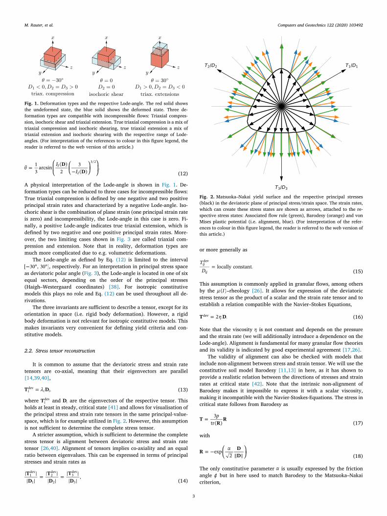
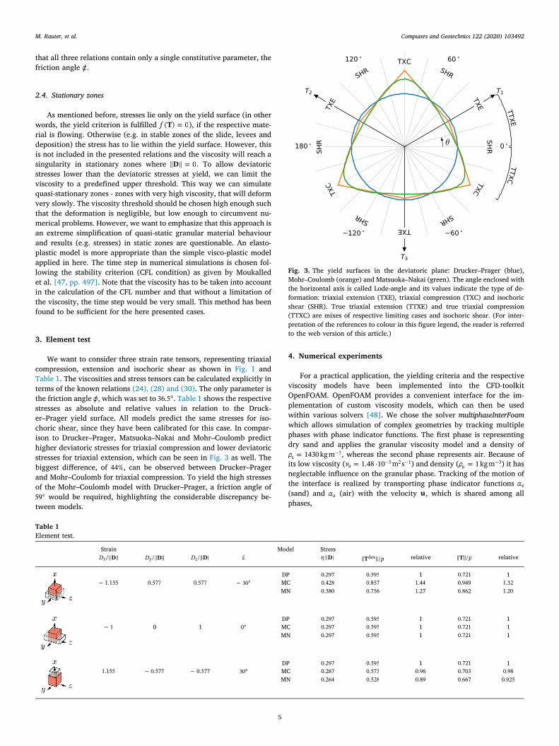
A physical interpretation of the Lode-angle is shown in Fig. 1. De-formation types can be reduced to three cases for incompressible flows:True triaxial compression is defined by one negative and two positiveprincipal strain rates and characterized by a negative Lode-angle. Iso-choric shear is the combination of plane strain (one principal strain rateis zero) and incompressibility, the Lode-angle in this case is zero. Fi-nally, a positive Lode-angle indicates true triaxial extension, which isdefined by two negative and one positive principal strain rates. More-over, the two limiting cases shown in Fig. 3 are called triaxial com-pression and extension. Note that in reality, deformation types aremuch more complicated due to e.g. volumetric deformations.

The Lode-angle as defined by Eq. (12) is limited to the interval° °[ 30 , 30 ], respectively. For an interpretation in principal stress space

as deviatoric polar angle (Fig. 3), the Lode-angle is located in one of sixequal sectors, depending on the order of the principal stresses(Haigh–Westergaard coordinates) [38]. For isotropic constitutivemodels this plays no role and Eq. (12) can be used throughout all de-rivations.

The three invariants are sufficient to describe a tensor, except for itsorientation in space (i.e. rigid body deformation). However, a rigidbody deformation is not relevant for isotropic constitutive models. Thismakes invariants very convenient for defining yield criteria and con-stitutive models.

2.2. Stress tensor reconstruction

It is common to assume that the deviatoric stress and strain ratetensors are co-axial, meaning that their eigenvectors are parallel[14,39,40],

=T D ,i i idev (13)

where Tidev and Di are the eigenvectors of the respective tensor. This

holds at least in steady, critical state [41] and allows for visualisation ofthe principal stress and strain rate tensors in the same principal-value-space, which is for example utilized in Fig. 2. However, this assumptionis not sufficient to determine the complete stress tensor.

A stricter assumption, which is sufficient to determine the completestress tensor is alignment between deviatoric stress and strain ratetensor [26,40]. Alignment of tensors implies co-axiality and an equalratio between eigenvalues. This can be expressed in terms of principalstresses and strain rates as

= =TD

TD

TD

,1dev

1

2dev

2

3dev

3 (14)

or more generally as

=TD

locally constant.ij

ij

dev

(15)

This assumption is commonly applied in granular flows, among othersby the µ I( )–rheology [26]. It allows for expression of the deviatoricstress tensor as the product of a scalar and the strain rate tensor and toestablish a relation compatible with the Navier–Stokes Equations,

=T D2 .dev (16)

Note that the viscosity is not constant and depends on the pressureand the strain rate (we will additionally introduce a dependence on theLode-angle). Alignment is fundamental for many granular flow theoriesand its validity is indicated by good experimental agreement [17,26].

The validity of alignment can also be checked with models thatinclude non-alignment between stress and strain tensor. We will use theconstitutive soil model Barodesy [11,13] in here, as it has shown toprovide a realistic relation between the directions of stresses and strainrates at critical state [42]. Note that the intrinsic non-alignment ofBarodesy makes it impossible to express it with a scalar viscosity,making it incompatible with the Navier-Stoskes-Equations. The stress incritical state follows from Barodesy as

= pTR

R3tr( ) (17)

with

=R DD

exp2

.(18)

The only constitutive parameter is usually expressed by the frictionangle but in here used to match Barodesy to the Matsuoka–Nakaicriterion,

Fig. 1. Deformation types and the respective Lode-angle. The red solid showsthe undeformed state, the blue solid shows the deformed state. Three de-formation types are compatible with incompressible flows: Triaxial compres-sion, isochoric shear and triaxial extension. True triaxial compression is a mix oftriaxial compression and isochoric shearing, true triaxial extension a mix oftriaxial extension and isochoric shearing with the respective range of Lode-angles. (For interpretation of the references to colour in this figure legend, thereader is referred to the web version of this article.)

Fig. 2. Matsuoka–Nakai yield surface and the respective principal stresses(black) in the deviatoric plane of principal stress/strain space. The strain rates,which can create these stress states are shown as arrows, attached to the re-spective stress states: Associated flow rule (green), Barodesy (orange) and vonMises plastic potential (i.e. alignment, blue). (For interpretation of the refer-ences to colour in this figure legend, the reader is referred to the web version ofthis article.)

M. Rauter, et al. Computers and Geotechnics 122 (2020) 103492

3

=+

k k kk k k

23

log1 ( 1) ( 9)1 ( 1) ( 9)

,MN MN MN

MN MN MN (19)

where kMN is the constitutive parameter of the Matsuoka–Nakai cri-terion, see Eq. (34). Note that the factor 2 in Eq. (18) is related to thedefinition of the norm following Eq. (8).

Furthermore, plasticity theory allows us to classify the popular ap-proach of alignment in a broader context. The associated flow rule,

= fD TT( ) , (20)

states that the plastic strain rate tensor (in here simply D, as we assumeideal plasticity) is oriented normal on the yield surface f T( ). This re-lation follows the principle of maximal plastic dissipation [4] but theyield surface f T( ) can be replaced with arbitrary plastic potentials f T( )in the flow rule (Eq. (20)). In such a case one speaks of a non-associativeflow rule. This procedure is applied often, as this matches soil beha-viour better [43–45].

Inserting the definition for alignment (Eq. (16)) into the flow rule(Eq. (20)) yields

= fT TT2( ) ,

dev

(21)

which necessarily leads to a von Mises type surface for the plastic po-tential,

= =f kT T( ) 0,dev 2vM (22)

with constant kvM. Conveniently, this flow rule is consistent with thecontinuity Eq. (2). Note, that associated flow rules for Drucker–Prager,Mohr–Coulomb and Matsuoka–Nakai predict volumetric strain, whichis contradicting with Eq. (2) and experimental observations in criticalstate. This gives three methods to determine the direction of the stresstensor with respect to the strain rate tensor: Associated flow rule (20)and von Mises plastic potential (i.e. alignment), as well as sophisticatedsoil models, in here Barodesy. All three approaches are presented andcompared in Fig. 2 for the Matsuoka–Nakai yield surface, as this mat-ches Barodesy best [12]. Results overlap in the deviatoric plane fortriaxial extension and compression but differ substantially for shear.The ad hoc assumption of alignment results in strain rate directionsclose to the associative flow rule and Barodesy, two physically rea-sonable models. In particular, the alignment assumption fits Barodesyand thus experimental behaviour, better than the associated flow rule.

In the following we will apply a von Mises plastic potential, as thisallows simple implementation of various yield surfaces into theNavier–Stokes equations. Moreover, this approach guarantees a welldefined stress tensor for all relevant yield surfaces and is compatiblewith incompressible flows.

2.3. Yield criteria

One of the simplest yield criteria, the von Mises yield surface hasbeen introduced in Eq. (22). It represents basic plastic behaviour and isas such the basis for visco-plastic rheologies like Bingham or Herschel-Bulkley [46]. However, it only takes into account the second stress-invariant and is thus not able to cover basic granular behaviour, i.e.pressure-dependent shear strength.

The Drucker–Prager yield criterion is the simplest criterion thattakes the frictional character of granular materials into account [29]. Assuch, it connects the pressure with the deviatoric part of the stresstensor,

= =f pT T( ) sin( ) 0,dev (23)

with the friction angle . Note that this is a special parametrisation for acohesionless material in terms of the friction angle , such thatDrucker–Prager and Mohr–Coulomb match for a Lode-angle = 0, i.e.

isochoric plane strain [14]. This yield surface allows us, in combinationwith the von Mises flow rule or equivalently Eq. (16), to define theviscosity as

= pD

sin( )2

.(24)

It is also possible to model the friction coefficient =µ sin( ) as afunction of the inertial number I, which leads to the µ I( )–rheology[26],

= µ I pD

( )2

.(25)

This shows that the µ I( )–rheology can be classified as a Drucker–Prageryield surface with a von Mises plastic potential, within the frameworkof plasticity theory.

The Mohr–Coulomb criterion additionally takes into account thedeformation type by incorporating both the major and minor principalstresses,

=+

=f T TT T

T( ) sin( ) 0.1 3

1 3 (26)

This relation can be expressed in terms of the Lode-angle and otherinvariants as [38]

= + =f I IT T T( ) sin( )3

cos( )sin( )

( ) 13

( ) 02dev

1(27)

and the viscosity follows as

=+

pD

sin( )2

33 cos( ) sin( ) sin( )

.(28)

Note that for = 0, i.e. isochoric shear, Eq. (28) reduces to Eq. (24).The Matsuoka–Nakai criterion is similar to the Mohr–Coulomb cri-

terion, however with a continuous, smooth yield surface. It is defined as

= =f I II

kT T TT

( ) ( ) ( )( )

0.1 2

3MN (29)

Introducing Eq. (16) into Eq. (29) leads to a viscosity that representsthis yield surface,

=

° <

< °

=

p a

p a

for 30 0,

for 0 30 ,

for 0,p kkD

cos( ) 3 sin( ) 16

2cos( ) 16

293

MNMN (30)

with

=a I kI kD

D( )(3 )

( ),2 MN

3 MN (31)

=b kI kD9

( ),MN

3 MN (32)

=+a b b

a b13

arctan3 3(4 27 )

2 27.

3 2

3(33)

The first case in Eq. (30) corresponds to true triaxial extension, thesecond case to true triaxial compression and the last case to isochoricshear, where =I D( ) 03 . The constant kMN is usually chosen such thatMatsuoka–Nakai fits the Mohr–Coulomb criterion for triaxial extensionand compression, i.e. for = ± °30 . Alternatively, kMN can be chosensuch that it fits Mohr–Coulomb and Drucker–Prager for isochoric shear( = 0),

=k 9 3 sin ( )1 sin ( )

.MN2

2 (34)

This is more appropriate for granular flows, as we will show later. Note

M. Rauter, et al. Computers and Geotechnics 122 (2020) 103492

4

that all three relations contain only a single constitutive parameter, thefriction angle .

2.4. Stationary zones

As mentioned before, stresses lie only on the yield surface (in otherwords, the yield criterion is fulfilled =f T( ) 0), if the respective mate-rial is flowing. Otherwise (e.g. in stable zones of the slide, levees anddeposition) the stress has to lie within the yield surface. However, thisis not included in the presented relations and the viscosity will reach asingularity in stationary zones where =D 0. To allow deviatoricstresses lower than the deviatoric stresses at yield, we can limit theviscosity to a predefined upper threshold. This way we can simulatequasi-stationary zones - zones with very high viscosity, that will deformvery slowly. The viscosity threshold should be chosen high enough suchthat the deformation is negligible, but low enough to circumvent nu-merical problems. However, we want to emphasize that this approach isan extreme simplification of quasi-static granular material behaviourand results (e.g. stresses) in static zones are questionable. An elasto-plastic model is more appropriate than the simple visco-plastic modelapplied in here. The time step in numerical simulations is chosen fol-lowing the stability criterion (CFL condition) as given by Moukalledet al. [47, pp. 497]. Note that the viscosity has to be taken into accountin the calculation of the CFL number and that without a limitation ofthe viscosity, the time step would be very small. This method has beenfound to be sufficient for the here presented cases.

3. Element test

We want to consider three strain rate tensors, representing triaxialcompression, extension and isochoric shear as shown in Fig. 1 andTable 1. The viscosities and stress tensors can be calculated explicitly interms of the known relations (24), (28) and (30). The only parameter isthe friction angle , which was set to °36.5 . Table 1 shows the respectivestresses as absolute and relative values in relation to the Druck-er–Prager yield surface. All models predict the same stresses for iso-choric shear, since they have been calibrated for this case. In compar-ison to Drucker–Prager, Matsuoka–Nakai and Mohr–Coulomb predicthigher deviatoric stresses for triaxial compression and lower deviatoricstresses for triaxial extension, which can be seen in Fig. 3 as well. Thebiggest difference, of 44%, can be observed between Drucker–Pragerand Mohr–Coulomb for triaxial compression. To yield the high stressesof the Mohr–Coulomb model with Drucker–Prager, a friction angle of

°59 would be required, highlighting the considerable discrepancy be-tween models.

4. Numerical experiments

For a practical application, the yielding criteria and the respectiveviscosity models have been implemented into the CFD-toolkitOpenFOAM. OpenFOAM provides a convenient interface for the im-plementation of custom viscosity models, which can then be usedwithin various solvers [48]. We chose the solver multiphaseInterFoamwhich allows simulation of complex geometries by tracking multiplephases with phase indicator functions. The first phase is representingdry sand and applies the granular viscosity model and a density of

= 1430 kg ms3, whereas the second phase represents air. Because of

its low viscosity ( = 1.48 ·10 m sa5 2 1) and density ( = 1 kg ma

3) it hasneglectable influence on the granular phase. Tracking of the motion ofthe interface is realized by transporting phase indicator functions s(sand) and a (air) with the velocity u, which is shared among allphases,

Table 1Element test.

Strain Model StressD D/x D D/y D D/z D pT /dev relative pT / relative

DP 0.297 0.595 1 0.721 11.155 0.577 0.577 °30 MC 0.428 0.857 1.44 0.949 1.32

MN 0.380 0.756 1.27 0.862 1.20

DP 0.297 0.595 1 0.721 11 0 1 °0 MC 0.297 0.595 1 0.721 1

MN 0.297 0.595 1 0.721 1

DP 0.297 0.595 1 0.721 11.155 0.577 0.577 °30 MC 0.287 0.573 0.96 0.703 0.98

MN 0.264 0.528 0.89 0.667 0.925

Fig. 3. The yield surfaces in the deviatoric plane: Drucker–Prager (blue),Mohr–Coulomb (orange) and Matsuoka–Nakai (green). The angle enclosed withthe horizontal axis is called Lode-angle and its values indicate the type of de-formation: triaxial extension (TXE), triaxial compression (TXC) and isochoricshear (SHR). True triaxial extension (TTXE) and true triaxial compression(TTXC) are mixes of respective limiting cases and isochoric shear. (For inter-pretation of the references to colour in this figure legend, the reader is referredto the web version of this article.)

M. Rauter, et al. Computers and Geotechnics 122 (2020) 103492

5

+ =t

u· 0.ii (35)

With known phase indicator values i (i being either s or a), the localdensity and viscosity can be calculated as the mean of individualphase values, i.e.

= ,i

i i(36)

= .i

i i(37)

This results in a simple model for granular flows with complex geo-metries and large strain. We apply a friction angle of = °36.5 in allsimulations, similar to Savage et al. [49]. The viscosity is truncated tothe interval = [10 , 10 ] m ss

5 0 2 1.The simplest and most common benchmarks for granular flow

models are two-dimensional column collapses, flows on inclined planesand flows down chutes. However, they all lead to isochoric plane strainconditions and are therefore inappropriate for our investigations. Asshown with the simple element test, all models will yield the sameresults in two-dimensional simulations. This behaviour has been con-firmed with back-calculations of the experiments by Balmforth andKerswell [50]. Results are not shown here as they basically matchprevious results of e.g. Lagrée et al. [51] and Savage et al. [49]. Itfollows that for a meaningful comparison of the proposed rheologies,we need to induce three-dimensional deformations. Axisymmetric si-mulations are an obvious choice for such a task, as they enforce three-dimensional deformations while keeping computational expense com-parable to a two-dimensional case.

4.1. Cylindrical granular collapse

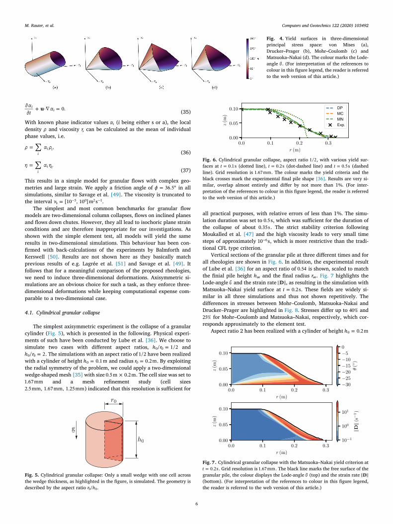
The simplest axisymmetric experiment is the collapse of a granularcylinder (Fig. 5), which is presented in the following. Physical experi-ments of such have been conducted by Lube et al. [36]. We choose tosimulate two cases with different aspect ratios, =h r/ 1/20 0 and

=h r/ 20 0 . The simulations with an aspect ratio of 1/2 have been realizedwith a cylinder of height =h 0.1 m0 and radius =r 0.2m0 . By exploitingthe radial symmetry of the problem, we could apply a two-dimensionalwedge-shaped mesh [35] with size ×0.5 m 0.2 m. The cell size was set to1.67mm and a mesh refinement study (cell sizes2.5mm, 1.67mm, 1.25mm) indicated that this resolution is sufficient for

all practical purposes, with relative errors of less than 1%. The simu-lation duration was set to 0.5 s, which was sufficient for the duration ofthe collapse of about 0.35s. The strict stability criterion followingMoukalled et al. [47] and the high viscosity leads to very small timesteps of approximately 10 s6 , which is more restrictive than the tradi-tional CFL type criterion.

Vertical sections of the granular pile at three different times and forall rheologies are shown in Fig. 6. In addition, the experimental resultof Lube et al. [36] for an aspect ratio of 0.54 is shown, scaled to matchthe finial pile height h and the final radius r . Fig. 7 highlights theLode-angle and the strain rate D , as resulting in the simulation withMatsuoka–Nakai yield surface at =t 0.2s. These fields are widely si-milar in all three simulations and thus not shown repetitively. Thedifferences in stresses between Mohr–Coulomb, Matsuoka–Nakai andDrucker–Prager are highlighted in Fig. 8. Stresses differ up to 40% and25% for Mohr–Coulomb and Matsuoka–Nakai, respectively, which cor-responds approximately to the element test.

Aspect ratio 2 has been realized with a cylinder of height =h 0.2 m0

Fig. 4. Yield surfaces in three-dimensionalprincipal stress space: von Mises (a),Drucker–Prager (b), Mohr–Coulomb (c) andMatsuoka–Nakai (d). The colour marks the Lode-angle . (For interpretation of the references tocolour in this figure legend, the reader is referredto the web version of this article.)

Fig. 5. Cylindrical granular collapse: Only a small wedge with one cell acrossthe wedge thickness, as highlighted in the figure, is simulated. The geometry isdescribed by the aspect ratio r h/0 0.

Fig. 6. Cylindrical granular collapse, aspect ratio 1/2, with various yield sur-faces at =t 0.1s (dotted line), =t 0.2s (dot-dashed line) and =t 0.5s (dashedline). Grid resolution is 1.67mm. The colour marks the yield criteria and theblack crosses mark the experimental final pile shape [36]. Results are very si-milar, overlap almost entirely and differ by not more than 1%. (For inter-pretation of the references to colour in this figure legend, the reader is referredto the web version of this article.)

Fig. 7. Cylindrical granular collapse with the Matsuoka–Nakai yield criterion at=t 0.2s. Grid resolution is 1.67mm. The black line marks the free surface of the

granular pile, the colour displays the Lode-angle (top) and the strain rate D(bottom). (For interpretation of the references to colour in this figure legend,the reader is referred to the web version of this article.)

M. Rauter, et al. Computers and Geotechnics 122 (2020) 103492

6

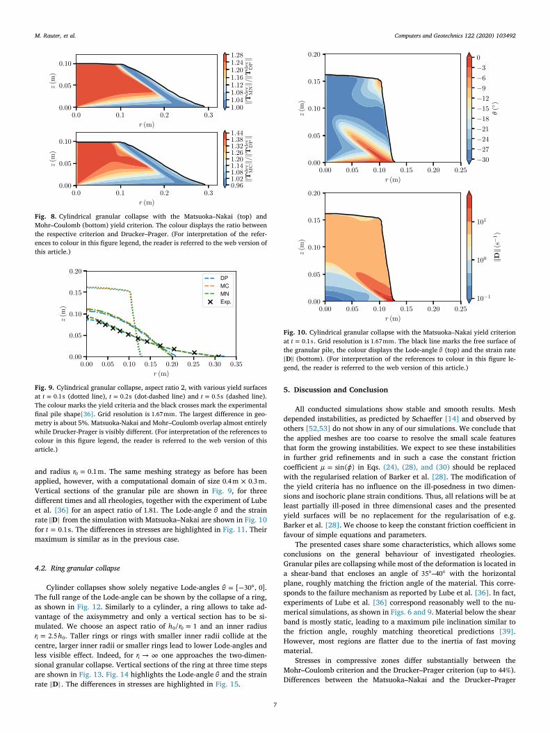
and radius =r 0.1m0 . The same meshing strategy as before has beenapplied, however, with a computational domain of size ×0.4 m 0.3 m.Vertical sections of the granular pile are shown in Fig. 9, for threedifferent times and all rheologies, together with the experiment of Lubeet al. [36] for an aspect ratio of 1.81. The Lode-angle and the strainrate D from the simulation with Matsuoka–Nakai are shown in Fig. 10for =t 0.1s. The differences in stresses are highlighted in Fig. 11. Theirmaximum is similar as in the previous case.

4.2. Ring granular collapse

Cylinder collapses show solely negative Lode-angles = °[ 30 , 0].The full range of the Lode-angle can be shown by the collapse of a ring,as shown in Fig. 12. Similarly to a cylinder, a ring allows to take ad-vantage of the axisymmetry and only a vertical section has to be si-mulated. We choose an aspect ratio of =h r/ 10 0 and an inner radius

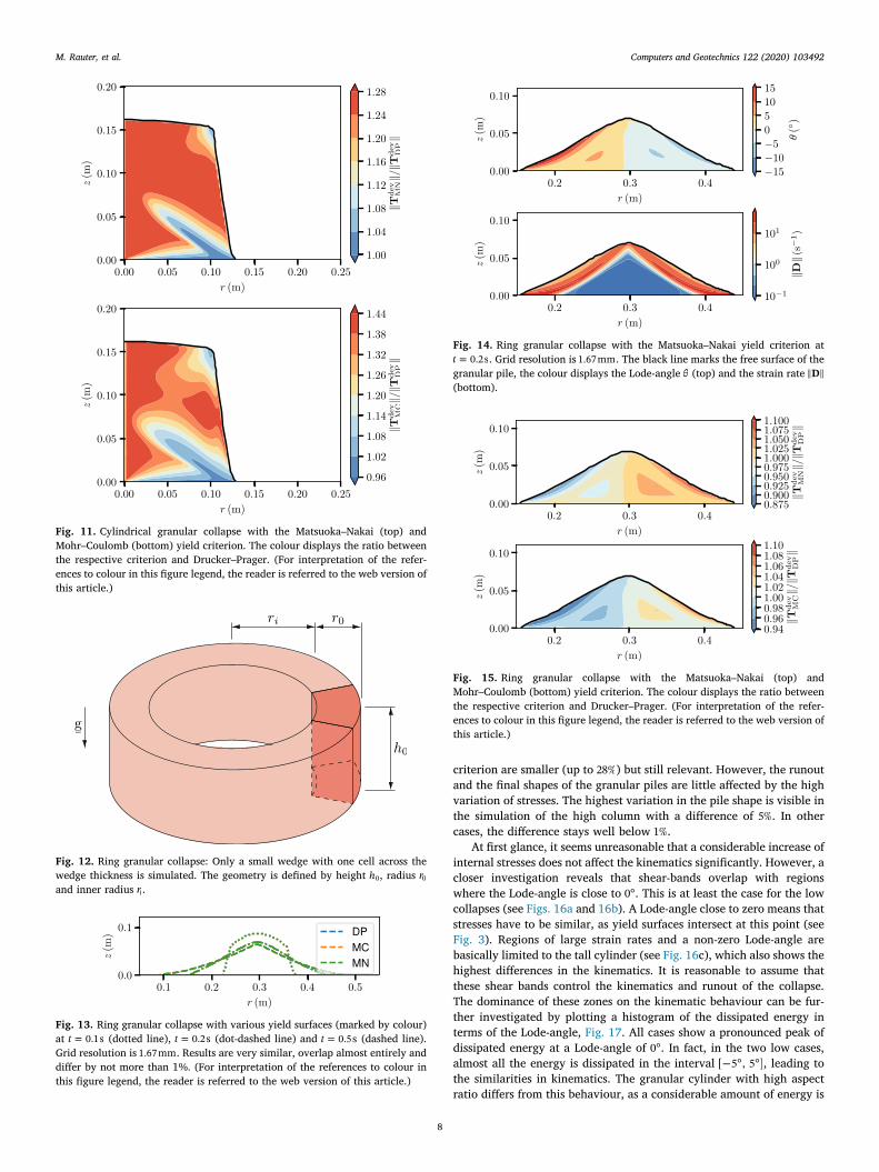
=r h2.5i 0. Taller rings or rings with smaller inner radii collide at thecentre, larger inner radii or smaller rings lead to lower Lode-angles andless visible effect. Indeed, for ri one approaches the two-dimen-sional granular collapse. Vertical sections of the ring at three time stepsare shown in Fig. 13. Fig. 14 highlights the Lode-angle and the strainrate D . The differences in stresses are highlighted in Fig. 15.

5. Discussion and Conclusion

All conducted simulations show stable and smooth results. Meshdepended instabilities, as predicted by Schaeffer [14] and observed byothers [52,53] do not show in any of our simulations. We conclude thatthe applied meshes are too coarse to resolve the small scale featuresthat form the growing instabilities. We expect to see these instabilitiesin further grid refinements and in such a case the constant frictioncoefficient =µ sin( ) in Eqs. (24), (28), and (30) should be replacedwith the regularised relation of Barker et al. [28]. The modification ofthe yield criteria has no influence on the ill-posedness in two dimen-sions and isochoric plane strain conditions. Thus, all relations will be atleast partially ill-posed in three dimensional cases and the presentedyield surfaces will be no replacement for the regularisation of e.g.Barker et al. [28]. We choose to keep the constant friction coefficient infavour of simple equations and parameters.

The presented cases share some characteristics, which allows someconclusions on the general behaviour of investigated rheologies.Granular piles are collapsing while most of the deformation is located ina shear-band that encloses an angle of °35 – °40 with the horizontalplane, roughly matching the friction angle of the material. This corre-sponds to the failure mechanism as reported by Lube et al. [36]. In fact,experiments of Lube et al. [36] correspond reasonably well to the nu-merical simulations, as shown in Figs. 6 and 9. Material below the shearband is mostly static, leading to a maximum pile inclination similar tothe friction angle, roughly matching theoretical predictions [39].However, most regions are flatter due to the inertia of fast movingmaterial.

Stresses in compressive zones differ substantially between theMohr–Coulomb criterion and the Drucker–Prager criterion (up to 44%).Differences between the Matsuoka–Nakai and the Drucker–Prager

Fig. 8. Cylindrical granular collapse with the Matsuoka–Nakai (top) andMohr–Coulomb (bottom) yield criterion. The colour displays the ratio betweenthe respective criterion and Drucker–Prager. (For interpretation of the refer-ences to colour in this figure legend, the reader is referred to the web version ofthis article.)

Fig. 9. Cylindrical granular collapse, aspect ratio 2, with various yield surfacesat =t 0.1s (dotted line), =t 0.2s (dot-dashed line) and =t 0.5s (dashed line).The colour marks the yield criteria and the black crosses mark the experimentalfinal pile shape[36]. Grid resolution is 1.67mm. The largest difference in geo-metry is about 5%. Matsuoka-Nakai and Mohr–Coulomb overlap almost entirelywhile Drucker-Prager is visibly different. (For interpretation of the references tocolour in this figure legend, the reader is referred to the web version of thisarticle.)

Fig. 10. Cylindrical granular collapse with the Matsuoka–Nakai yield criterionat =t 0.1s. Grid resolution is 1.67mm. The black line marks the free surface ofthe granular pile, the colour displays the Lode-angle (top) and the strain rateD (bottom). (For interpretation of the references to colour in this figure le-

gend, the reader is referred to the web version of this article.)

M. Rauter, et al. Computers and Geotechnics 122 (2020) 103492

7

criterion are smaller (up to 28%) but still relevant. However, the runoutand the final shapes of the granular piles are little affected by the highvariation of stresses. The highest variation in the pile shape is visible inthe simulation of the high column with a difference of 5%. In othercases, the difference stays well below 1%.

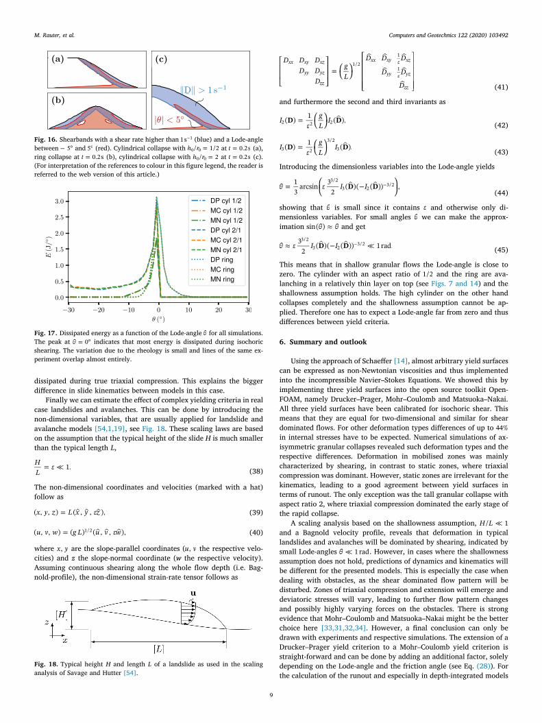
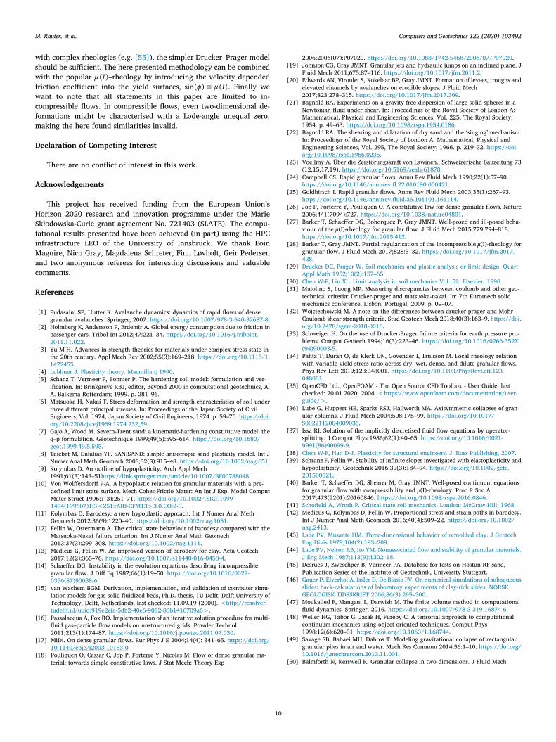
At first glance, it seems unreasonable that a considerable increase ofinternal stresses does not affect the kinematics significantly. However, acloser investigation reveals that shear-bands overlap with regionswhere the Lode-angle is close to °0 . This is at least the case for the lowcollapses (see Figs. 16a and 16b). A Lode-angle close to zero means thatstresses have to be similar, as yield surfaces intersect at this point (seeFig. 3). Regions of large strain rates and a non-zero Lode-angle arebasically limited to the tall cylinder (see Fig. 16c), which also shows thehighest differences in the kinematics. It is reasonable to assume thatthese shear bands control the kinematics and runout of the collapse.The dominance of these zones on the kinematic behaviour can be fur-ther investigated by plotting a histogram of the dissipated energy interms of the Lode-angle, Fig. 17. All cases show a pronounced peak ofdissipated energy at a Lode-angle of °0 . In fact, in the two low cases,almost all the energy is dissipated in the interval ° °[ 5 , 5 ], leading tothe similarities in kinematics. The granular cylinder with high aspectratio differs from this behaviour, as a considerable amount of energy is

Fig. 11. Cylindrical granular collapse with the Matsuoka–Nakai (top) andMohr–Coulomb (bottom) yield criterion. The colour displays the ratio betweenthe respective criterion and Drucker–Prager. (For interpretation of the refer-ences to colour in this figure legend, the reader is referred to the web version ofthis article.)

Fig. 12. Ring granular collapse: Only a small wedge with one cell across thewedge thickness is simulated. The geometry is defined by height h0, radius r0and inner radius ri.

Fig. 13. Ring granular collapse with various yield surfaces (marked by colour)at =t 0.1s (dotted line), =t 0.2s (dot-dashed line) and =t 0.5s (dashed line).Grid resolution is 1.67mm. Results are very similar, overlap almost entirely anddiffer by not more than 1%. (For interpretation of the references to colour inthis figure legend, the reader is referred to the web version of this article.)

Fig. 14. Ring granular collapse with the Matsuoka–Nakai yield criterion at=t 0.2s. Grid resolution is 1.67mm. The black line marks the free surface of the

granular pile, the colour displays the Lode-angle (top) and the strain rate D(bottom).

Fig. 15. Ring granular collapse with the Matsuoka–Nakai (top) andMohr–Coulomb (bottom) yield criterion. The colour displays the ratio betweenthe respective criterion and Drucker–Prager. (For interpretation of the refer-ences to colour in this figure legend, the reader is referred to the web version ofthis article.)

M. Rauter, et al. Computers and Geotechnics 122 (2020) 103492

8

dissipated during true triaxial compression. This explains the biggerdifference in slide kinematics between models in this case.

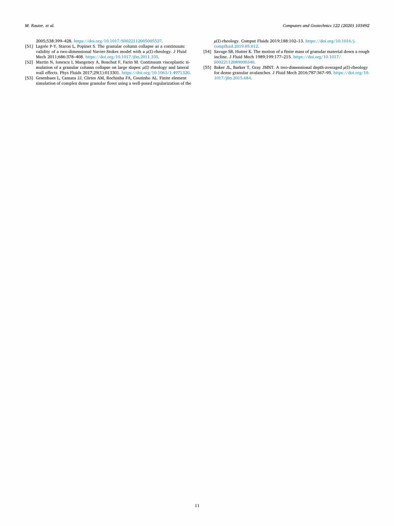
Finally we can estimate the effect of complex yielding criteria in realcase landslides and avalanches. This can be done by introducing thenon-dimensional variables, that are usually applied for landslide andavalanche models [54,1,19], see Fig. 18. These scaling laws are basedon the assumption that the typical height of the slide H is much smallerthan the typical length L,

=HL

1. (38)

The non-dimensional coordinates and velocities (marked with a hat)follow as

=x y z L x y z( , , ) ( , , ), (39)

=u v w g L u v w( , , ) ( ) ( , , ),1/2 (40)

where x y, are the slope-parallel coordinates (u v, the respective velo-cities) and z the slope-normal coordinate (w the respective velocity).Assuming continuous shearing along the whole flow depth (i.e. Bag-nold-profile), the non-dimensional strain-rate tensor follows as

=D D D

D DD

gL

D D D

D D

D

xx xy xz

yy yz

zz

xx xy xz

yy yz

zz

1/2

1

1

(41)

and furthermore the second and third invariants as

=I gL

ID D( ) 1 ( ),2 2 2 (42)

=I gL

ID D( ) 1 ( ).3 2

3/23 (43)

Introducing the dimensionless variables into the Lode-angle yields

= I ID D13

arcsin 32

( )( ( )) ,3/2

3 23/2

(44)

showing that is small since it contains and otherwise only di-mensionless variables. For small angles we can make the approx-imation sin( ) and get

I ID D32

( )( ( )) 1rad.3/2

3 23/2

(45)

This means that in shallow granular flows the Lode-angle is close tozero. The cylinder with an aspect ratio of 1/2 and the ring are ava-lanching in a relatively thin layer on top (see Figs. 7 and 14) and theshallowness assumption holds. The high cylinder on the other handcollapses completely and the shallowness assumption cannot be ap-plied. Therefore one has to expect a Lode-angle far from zero and thusdifferences between yield criteria.

6. Summary and outlook

Using the approach of Schaeffer [14], almost arbitrary yield surfacescan be expressed as non-Newtonian viscosities and thus implementedinto the incompressible Navier–Stokes Equations. We showed this byimplementing three yield surfaces into the open source toolkit Open-FOAM, namely Drucker–Prager, Mohr–Coulomb and Matsuoka–Nakai.All three yield surfaces have been calibrated for isochoric shear. Thismeans that they are equal for two-dimensional and similar for sheardominated flows. For other deformation types differences of up to 44%in internal stresses have to be expected. Numerical simulations of ax-isymmetric granular collapses revealed such deformation types and therespective differences. Deformation in mobilised zones was mainlycharacterized by shearing, in contrast to static zones, where triaxialcompression was dominant. However, static zones are irrelevant for thekinematics, leading to a good agreement between yield surfaces interms of runout. The only exception was the tall granular collapse withaspect ratio 2, where triaxial compression dominated the early stage ofthe rapid collapse.

A scaling analysis based on the shallowness assumption, H L/ 1and a Bagnold velocity profile, reveals that deformation in typicallandslides and avalanches will be dominated by shearing, indicated bysmall Lode-angles 1 rad. However, in cases where the shallownessassumption does not hold, predictions of dynamics and kinematics willbe different for the presented models. This is especially the case whendealing with obstacles, as the shear dominated flow pattern will bedisturbed. Zones of triaxial compression and extension will emerge anddeviatoric stresses will vary, leading to further flow pattern changesand possibly highly varying forces on the obstacles. There is strongevidence that Mohr–Coulomb and Matsuoka–Nakai might be the betterchoice here [33,31,32,34]. However, a final conclusion can only bedrawn with experiments and respective simulations. The extension of aDrucker–Prager yield criterion to a Mohr–Coulomb yield criterion isstraight-forward and can be done by adding an additional factor, solelydepending on the Lode-angle and the friction angle (see Eq. (28)). Forthe calculation of the runout and especially in depth-integrated models

Fig. 16. Shearbands with a shear rate higher than 1 s 1 (blue) and a Lode-anglebetween °5 and °5 (red). Cylindrical collapse with =h r/ 1/20 0 at =t 0.2s (a),ring collapse at =t 0.2s (b), cylindrical collapse with =h r/ 20 0 at =t 0.2s (c).(For interpretation of the references to colour in this figure legend, the reader isreferred to the web version of this article.)

Fig. 17. Dissipated energy as a function of the Lode-angle for all simulations.The peak at = °0 indicates that most energy is dissipated during isochoricshearing. The variation due to the rheology is small and lines of the same ex-periment overlap almost entirely.

Fig. 18. Typical height H and length L of a landslide as used in the scalinganalysis of Savage and Hutter [54].

M. Rauter, et al. Computers and Geotechnics 122 (2020) 103492

9

with complex rheologies (e.g. [55]), the simpler Drucker–Prager modelshould be sufficient. The here presented methodology can be combinedwith the popular µ I( )–rheology by introducing the velocity dependedfriction coefficient into the yield surfaces, µ Isin( ) ( ). Finally wewant to note that all statements in this paper are limited to in-compressible flows. In compressible flows, even two-dimensional de-formations might be characterised with a Lode-angle unequal zero,making the here found similarities invalid.

Declaration of Competing Interest

There are no conflict of interest in this work.

Acknowledgements

This project has received funding from the European Union’sHorizon 2020 research and innovation programme under the MarieSkłodowska-Curie grant agreement No. 721403 (SLATE). The compu-tational results presented have been achieved (in part) using the HPCinfrastructure LEO of the University of Innsbruck. We thank EoinMaguire, Nico Gray, Magdalena Schreter, Finn Løvholt, Geir Pedersenand two anonymous referees for interesting discussions and valuablecomments.

References

[1] Pudasaini SP, Hutter K. Avalanche dynamics: dynamics of rapid flows of densegranular avalanches. Springer; 2007. https://doi.org/10.1007/978-3-540-32687-8.

[2] Holmberg K, Andersson P, Erdemir A. Global energy consumption due to friction inpassenger cars. Tribol Int 2012;47:221–34. https://doi.org/10.1016/j.triboint.2011.11.022.

[3] Yu M-H. Advances in strength theories for materials under complex stress state inthe 20th century. Appl Mech Rev 2002;55(3):169–218. https://doi.org/10.1115/1.1472455.

[4] Lubliner J. Plasticity theory. Macmillan; 1990.[5] Schanz T, Vermeer P, Bonnier P. The hardening soil model: formulation and ver-

ification. In: Brinkgreve RBJ, editor, Beyond 2000 in computational geotechnics, A.A. Balkema Rotterdam; 1999. p. 281–96.

[6] Matsuoka H, Nakai T. Stress-deformation and strength characteristics of soil underthree different principal stresses. In: Proceedings of the Japan Society of CivilEngineers, Vol. 1974, Japan Society of Civil Engineers; 1974. p. 59–70. https://doi.org/10.2208/jscej1969.1974.232_59.

[7] Gajo A, Wood M. Severn-Trent sand: a kinematic-hardening constitutive model: theq–p formulation. Géotechnique 1999;49(5):595–614. https://doi.org/10.1680/geot.1999.49.5.595.

[8] Taiebat M, Dafalias YF. SANISAND: simple anisotropic sand plasticity model. Int JNumer Anal Meth Geomech 2008;32(8):915–48. https://doi.org/10.1002/nag.651.

[9] Kolymbas D. An outline of hypoplasticity. Arch Appl Mech1991;61(3):143–51https://link.springer.com/article/10.1007/BF00788048.

[10] Von Wolffersdorff P-A. A hypoplastic relation for granular materials with a pre-defined limit state surface. Mech Cohes-Frictio Mater: An Int J Exp, Model ComputMater Struct 1996;1(3):251–71. https://doi.org/10.1002/(SICI)1099-1484(199607)1:3<251::AID-CFM13>3.0.CO;2-3.

[11] Kolymbas D. Barodesy: a new hypoplastic approach. Int J Numer Anal MethGeomech 2012;36(9):1220–40. https://doi.org/10.1002/nag.1051.

[12] Fellin W, Ostermann A. The critical state behaviour of barodesy compared with theMatsuoka-Nakai failure criterion. Int J Numer Anal Meth Geomech2013;37(3):299–308. https://doi.org/10.1002/nag.1111.

[13] Medicus G, Fellin W. An improved version of barodesy for clay. Acta Geotech2017;12(2):365–76. https://doi.org/10.1007/s11440-016-0458-4.

[14] Schaeffer DG. Instability in the evolution equations describing incompressiblegranular flow. J Diff Eq 1987;66(1):19–50. https://doi.org/10.1016/0022-0396(87)90038-6.

[15] van Wachem BGM. Derivation, implementation, and validation of computer simu-lation models for gas-solid fluidized beds, Ph.D. thesis, TU Delft, Delft University ofTechnology, Delft, Netherlands, last checked: 11.09.19 (2000). <http://resolver.tudelft.nl/uuid:919e2efa-5db2-40e6-9082-83b1416709a6>.

[16] Passalacqua A, Fox RO. Implementation of an iterative solution procedure for multi-fluid gas–particle flow models on unstructured grids. Powder Technol2011;213(1):174–87. https://doi.org/10.1016/j.powtec.2011.07.030.

[17] MiDi. On dense granular flows. Eur Phys J E 2004;14(4): 341–65. https://doi.org/10.1140/epje/i2003-10153-0.

[18] Pouliquen O, Cassar C, Jop P, Forterre Y, Nicolas M. Flow of dense granular ma-terial: towards simple constitutive laws. J Stat Mech: Theory Exp

2006;2006(07):P07020. https://doi.org/10.1088/1742-5468/2006/07/P07020.[19] Johnson CG, Gray JMNT. Granular jets and hydraulic jumps on an inclined plane. J

Fluid Mech 2011;675:87–116. https://doi.org/10.1017/jfm.2011.2.[20] Edwards AN, Viroulet S, Kokelaar BP, Gray JMNT. Formation of levees, troughs and

elevated channels by avalanches on erodible slopes. J Fluid Mech2017;823:278–315. https://doi.org/10.1017/jfm.2017.309.

[21] Bagnold RA. Experiments on a gravity-free dispersion of large solid spheres in aNewtonian fluid under shear. In: Proceedings of the Royal Society of London A:Mathematical, Physical and Engineering Sciences, Vol. 225, The Royal Society;1954. p. 49–63. https://doi.org/10.1098/rspa.1954.0186.

[22] Bagnold RA. The shearing and dilatation of dry sand and the ‘singing’ mechanism.In: Proceedings of the Royal Society of London A: Mathematical, Physical andEngineering Sciences, Vol. 295, The Royal Society; 1966. p. 219–32. https://doi.org/10.1098/rspa.1966.0236.

[23] Voellmy A. Über die Zerstörungskraft von Lawinen., Schweizerische Bauzeitung 73(12,15,17,19). https://doi.org/10.5169/seals-61878.

[24] Campbell CS. Rapid granular flows. Annu Rev Fluid Mech 1990;22(1):57–90.https://doi.org/10.1146/annurev.fl.22.010190.000421.

[25] Goldhirsch I. Rapid granular flows. Annu Rev Fluid Mech 2003;35(1):267–93.https://doi.org/10.1146/annurev.fluid.35.101101.161114.

[26] Jop P, Forterre Y, Pouliquen O. A constitutive law for dense granular flows. Nature2006;441(7094):727. https://doi.org/10.1038/nature04801.

[27] Barker T, Schaeffer DG, Bohorquez P, Gray JMNT. Well-posed and ill-posed beha-viour of the μ(I)-rheology for granular flow. J Fluid Mech 2015;779:794–818.https://doi.org/10.1017/jfm.2015.412.

[28] Barker T, Gray JMNT. Partial regularisation of the incompressible μ(I)-rheology forgranular flow. J Fluid Mech 2017;828:5–32. https://doi.org/10.1017/jfm.2017.428.

[29] Drucker DC, Prager W. Soil mechanics and plastic analysis or limit design. QuartAppl Math 1952;10(2):157–65.

[30] Chen W-F, Liu XL. Limit analysis in soil mechanics Vol. 52. Elsevier; 1990.[31] Maiolino S, Luong MP. Measuring discrepancies between coulomb and other geo-

technical criteria: Drucker-prager and matsuoka-nakai. In: 7th Euromech solidmechanics conference, Lisbon, Portugal; 2009. p. 09–07.

[32] Wojciechowski M. A note on the differences between drucker-prager and Mohr-Coulomb shear strength criteria. Stud Geotech Mech 2018;40(3):163–9. https://doi.org/10.2478/sgem-2018-0016.

[33] Schweiger H. On the use of Drucker-Prager failure criteria for earth pressure pro-blems. Comput Geotech 1994;16(3):223–46. https://doi.org/10.1016/0266-352X(94)90003-5.

[34] Pähtz T, Durán O, de Klerk DN, Govender I, Trulsson M. Local rheology relationwith variable yield stress ratio across dry, wet, dense, and dilute granular flows.Phys Rev Lett 2019;123:048001. https://doi.org/10.1103/PhysRevLett.123.048001.

[35] OpenCFD Ltd., OpenFOAM - The Open Source CFD Toolbox - User Guide, lastchecked: 20.01.2020; 2004. <https://www.openfoam.com/documentation/user-guide/>.

[36] Lube G, Huppert HE, Sparks RSJ, Hallworth MA. Axisymmetric collapses of gran-ular columns. J Fluid Mech 2004;508:175–99. https://doi.org/10.1017/S0022112004009036.

[37] Issa RI. Solution of the implicitly discretised fluid flow equations by operator-splitting. J Comput Phys 1986;62(1):40–65. https://doi.org/10.1016/0021-9991(86)90099-9.

[38] Chen W-F, Han D-J. Plasticity for structural engineers. J. Ross Publishing; 2007.[39] Schranz F, Fellin W. Stability of infinite slopes investigated with elastoplasticity and

hypoplasticity. Geotechnik 2016;39(3):184–94. https://doi.org/10.1002/gete.201500021.

[40] Barker T, Schaeffer DG, Shearer M, Gray JMNT. Well-posed continuum equationsfor granular flow with compressibility and μ(I)-rheology. Proc R Soc A2017;473(2201):20160846. https://doi.org/10.1098/rspa.2016.0846.

[41] Schofield A, Wroth P. Critical state soil mechanics. London: McGraw-Hill; 1968.[42] Medicus G, Kolymbas D, Fellin W. Proportional stress and strain paths in barodesy.

Int J Numer Anal Meth Geomech 2016;40(4):509–22. https://doi.org/10.1002/nag.2413.

[43] Lade PV, Musante HM. Three-dimensional behavior of remolded clay. J GeotechEng Divis 1978;104(2):193–209.

[44] Lade PV, Nelson RB, Ito YM. Nonassociated flow and stability of granular materials.J Eng Mech 1987;113(9):1302–18.

[45] Desrues J, Zweschper B, Vermeer PA. Database for tests on Hostun RF sand,Publication Series of the Institute of Geotechnik, University Stuttgart.

[46] Gauer P, Elverhoi A, Issler D, De Blasio FV. On numerical simulations of subaqueousslides: back-calculations of laboratory experiments of clay-rich slides. NORSKGEOLOGISK TIDSSKRIFT 2006;86(3):295–300.

[47] Moukalled F, Mangani L, Darwish M. The finite volume method in computationalfluid dynamics. Springer; 2016. https://doi.org/10.1007/978-3-319-16874-6.

[48] Weller HG, Tabor G, Jasak H, Fureby C. A tensorial approach to computationalcontinuum mechanics using object-oriented techniques. Comput Phys1998;12(6):620–31. https://doi.org/10.1063/1.168744.

[49] Savage SB, Babaei MH, Dabros T. Modeling gravitational collapse of rectangulargranular piles in air and water. Mech Res Commun 2014;56:1–10. https://doi.org/10.1016/j.mechrescom.2013.11.001.

[50] Balmforth N, Kerswell R. Granular collapse in two dimensions. J Fluid Mech

M. Rauter, et al. Computers and Geotechnics 122 (2020) 103492

10

2005;538:399–428. https://doi.org/10.1017/S0022112005005537.[51] Lagrée P-Y, Staron L, Popinet S. The granular column collapse as a continuum:

validity of a two-dimensional Navier-Stokes model with a μ(I)-rheology. J FluidMech 2011;686:378–408. https://doi.org/10.1017/jfm.2011.335.

[52] Martin N, Ionescu I, Mangeney A, Bouchut F, Farin M. Continuum viscoplastic si-mulation of a granular column collapse on large slopes: μ(I) rheology and lateralwall effects. Phys Fluids 2017;29(1):013301. https://doi.org/10.1063/1.4971320.

[53] Gesenhues L, Camata JJ, Côrtes AM, Rochinha FA, Coutinho AL. Finite elementsimulation of complex dense granular flows using a well-posed regularization of the

μ(I)-rheology. Comput Fluids 2019;188:102–13. https://doi.org/10.1016/j.compfluid.2019.05.012.

[54] Savage SB, Hutter K. The motion of a finite mass of granular material down a roughincline. J Fluid Mech 1989;199:177–215. https://doi.org/10.1017/S0022112089000340.

[55] Baker JL, Barker T, Gray JMNT. A two-dimensional depth-averaged μ(I)-rheologyfor dense granular avalanches. J Fluid Mech 2016;787:367–95. https://doi.org/10.1017/jfm.2015.684.

M. Rauter, et al. Computers and Geotechnics 122 (2020) 103492

11