High-Performance Analysis of Filtered Semantic

Graphs

Aydin BulucArmando FoxJohn GilbertShoaib Ashraf KamilAdam LugowskiLeonid OlikerSamuel Williams

Electrical Engineering and Computer SciencesUniversity of California at Berkeley

Technical Report No. UCB/EECS-2012-61

http://www.eecs.berkeley.edu/Pubs/TechRpts/2012/EECS-2012-61.html

May 6, 2012

Copyright © 2012, by the author(s).All rights reserved.

Permission to make digital or hard copies of all or part of this work forpersonal or classroom use is granted without fee provided that copies arenot made or distributed for profit or commercial advantage and that copiesbear this notice and the full citation on the first page. To copy otherwise, torepublish, to post on servers or to redistribute to lists, requires prior specificpermission.

High-Performance Analysis of Filtered Semantic Graphs

Aydın Buluç§∗abuluc@lbl.gov

Armando Fox‡fox@cs.berkeley.edu

John R. Gilbert†gilbert@cs.ucsb.edu

Shoaib Kamil‡∗skamil@cs.berkeley.edu

Adam Lugowski†∗alugowski@cs.ucsb.edu

Leonid Oliker§loliker@lbl.gov

Samuel Williams§swwilliams@lbl.gov

§CRDLawrence Berkeley Nat. Lab.

Berkeley, CA 94720

† Dept. of Computer ScienceUniversity of California

Santa Barbara, CA 93106

‡EECS Dept.University of CaliforniaBerkeley, CA 94720

ABSTRACTHigh performance is a crucial consideration when executinga complex analytic query on a massive semantic graph. In asemantic graph, vertices and edges carry “attributes” of var-ious types. Analytic queries on semantic graphs typicallydepend on the values of these attributes; thus, the com-putation must either view the graph through a filter thatpasses only those individual vertices and edges of interest,or else must first materialize a subgraph or subgraphs con-sisting of only the vertices and edges of interest. The filteredapproach is superior due to its generality, ease of use, andmemory efficiency, but may carry a performance cost.

In the Knowledge Discovery Toolbox (KDT), a Pythonlibrary for parallel graph computations, the user writes fil-ters in a high-level language, but those filters result in rel-atively low performance due to the bottleneck of having tocall into the Python interpreter for each edge. In this work,we use the Selective Embedded JIT Specialization (SEJITS)approach to automatically translate filters defined by pro-grammers into a lower-level efficiency language, bypassingthe upcall into Python. We evaluate our approach by com-paring it with the high-performance C++ /MPI Combinato-rial BLAS engine, and show that the productivity gained byusing a high-level filtering language comes without sacrific-ing performance. We also present a new roofline model forgraph traversals, and show that our high-performance im-plementations do not significantly deviate from the roofline.

1. INTRODUCTION

1.1 MotivationLarge-scale graph analytics are a central requirement of

bioinformatics, finance, social network analysis, national se-curity, and many other fields. Going beyond simple searches,analysts use high-performance computing systems to exe-cute complex graph algorithms on large corpora of data.Often, a large semantic graph is built up over time, withthe graph vertices representing entities of interest and theedges representing relationships of various kinds—for exam-ple, social network connections, financial transactions, orinterpersonal contacts.

∗Corresponding authors.

!"#$%&'&(#'%)$')%&(*+*,-#"#(

.%*/0('0&1%-(

213/)'&%#(2133)+"$*41+(5)//1%'(

6789:(.;5<&':(&'$=(

!"#'%">)'&?(213>"+*'1%"*,(@A;5(

Threading Support (OpenMP, Cilk, etc)

Graph experts

Domain scientists

B+1C,&?D&(!"#$1E&%-(F11,>1G(6B!F=(

SEJITS for performance

Graph Analysis Methodology

Figure 1: Overview of the high-performance graph-analysis software architecture described in this pa-per. KDT has graph abstractions and uses avery high-level language. Combinatorial BLAS hassparse linear-algebra abstractions, and geared to-wards performance.

In a semantic graph, edges and/or vertices are labeledwith attributes that may represent (for example) a time-stamp, a type of relationship, or a mode of communication.An analyst (i.e. a user of graph analytics) may want to runa complex workflow over a large graph, but wish to only usethose graph edges whose attributes pass a filter defined bythe analyst. For example, in a graph whose vertices repre-sent Twitter users and whose edges represent either “follow-ing” or “retweeting” relationships, the analyst may want tosearch through vertices reachable from a particular user viathe subgraph consisting only of “retweet” edges with time-stamps earlier than June 30.

The Knowledge Discovery Toolbox [19] is a flexible Python-based open-source toolkit for implementing complex graphalgorithms and executing them on high-performance paral-lel computers. KDT achieves high performance by invokingcomputational primitives supplied by a parallel C++ /MPIbackend, the Combinatorial BLAS [5]. This paper presentsnew work that allows KDT users to define filters in Python,which act to modify KDT’s action based on the attributesthat label individual edges or vertices.

Filters raise performance issues for large-scale graph anal-ysis. In many applications it is impossibly expensive to runa filter across an entire graph data corpus, materializing thefiltered graph as a new object for analysis. In addition to

the obvious storage problems with materialization, the timespent during materialization is typically not amortized bymany graph queries because the user modifies the query (orjust the filter) during interactive data analysis. The alter-native is to filter edges and vertices “on the fly” during exe-cution of the complex graph algorithm. A graph algorithmsexpert can implement an efficient on-the-fly filter as a set ofprimitive Combinatorial BLAS operations coded in C/C++ ;but filters written at the KDT level, as graph operations inPython, incur a significant performance penalty.

Our solution to this challenge is to apply Selective Just-In-Time Specialization techniques from the SEJITS approach [7].We define a semantic-graph-specific filter domain-specificlanguage (DSL), a subset of Python, and use SEJITS toimplement the specialization necessary for filters written inthat subset to execute as efficiently as low-level C code.

As a result, we are able to demonstrate that SEJITStechnology significantly accelerates Python graph analyticscodes written in KDT and running on clusters and multicoreCPUs. An overview of our approach is shown in Figure 1.

Figure 2 compares the performance of four filtering imple-mentations on a breadth-first search query in a graph with 8million vertices and 128 million edges. The chart shows timeto perform the query as we synthetically increase the portionof the graph that passes the filter on an input R-MAT [18]graph of scale 23, The top two lines are the methods im-plemented in the current release v0.2 of KDT [2]: slowestis materializing the subgraph before traversal, and next ison-the-fly filtering in Python. The third, red, line is ournew SEJITS+KDT implementation, which shows minimaloverhead and comes very close to the performance of nativeCombinatorial BLAS in the fourth line.

1.2 Main contributionsThe primary new contributions of this paper are:

1. A system design that allows domain-expert graph an-alysts to describe filtered semantic graph operations ina high-level language, using KDT v0.2.

2. An domain-specific language implementation that exe-cutes flexible filtering without sacrificing performance,using SEJITS selective compilation techniques.

3. Experimental demonstration of excellent performancescaling to graphs with millions of vertices and hundredsof millions of edges.

4. A new roofline performance model [24] for high-performancegraph computation, suitable for evaluating the perfor-mance of filtered semantic graph operations.

5. A detailed case study of the use of algebraic semir-ing operations as an alternative low-level approach tofiltering, using the Combinatorial BLAS.

1.3 Example of a filtered queryHere we present a simple example of a filtered query in a

semantic graph. We will refer to this example through thepaper, showing how the different implementations of filtersexpress the query and comparing their performance execut-ing it.

We consider a graph whose vertices are Twitter users, andwhose edges represent two different types of relationships be-tween users. In the first type, one user “follows” another; in

!"

#"

$"

%"

!&"

'#"

&$"

!(" !)(" #*(" !))("

!"#$%&'

(%)*

"%

'+,-".%/".*"#0+,+-1%

+,-"./012340546278" +,-" 9:;<-9=+,-" >?/@ABC9"

Figure 2: Performance of a filtered BFS query, com-paring four methods of implementing custom filters.The vertical axis is running time in seconds on alog scale; lower is better. From top to bottom, themethods are: materializing the filtered subgraph;on-the-fly filtering with high-level Python filters inKDT; on-the-fly filtering with high-level Python fil-ters specialized at runtime by SEJITS+KDT (thispaper’s main contribution); on-the-fly filtering withlow-level C++ filters implemented as customizedsemiring operations and compiled into Combinato-rial BLAS. The graph has 8 million vertices and 128million edges. The runs use 36 cores (4 sockets) ofIntel Xeon E7-8870 processors.

the second type, one user “retweets” another user’s tweet.Each retweet edge carries as attributes a timestamp and acount. Figure 3 shows a fragment of such a graph. Our ex-periments are with several semantic graphs, of various sizes,constructed from publicly available data on tweets during2009. The largest graph has about 17 million vertices and720 million edges. Section 7 describes the datasets in moredetail.

Our sample query is the one mentioned above: Given avertex of interest, determine the number of hops requiredto reach each other vertex by using only retweeting edgestimestamped earlier than June 30. The filter in this caseis a boolean predicate on edge attributes that defines thetypes and timestamps of the edges to be used. The query isa breadth-first search in the graph that ignores edges thatdo not pass the filter.

"

#

$

%&''&()*+<-23(224*+,9&:;)*27,+-./0,=72;8+>,

? !

@ A

BC

Figure 3: Graph of “following” and “retweeting” re-lationships. Black edges denote following, and rededges denote retweeting. Red edges are also labelledwith counts and timestamps, not shown.

1.4 Outline of the paperWe first survey related work. Then, Section 3 shows how

a filter can be implemented below the KDT level, as a user-specified semiring operation in the C++ /MPI Combinato-rial BLAS library that underlies KDT. This is a path to highperformance at the cost of usability: the analyst must trans-late the graph-attribute definition of the filter into low-levelC++ code for custom semiring scalar operations in Combi-natorial BLAS.

Section 4 describes the high-level filtering facility that isnew in Version 0.2 of KDT, in which filters are specified assimple Python predicates. This approach yields easy cus-tomization, and scales to many queries from many analystswithout demanding correspondingly many graph program-ming experts; however, it poses challenges to achieving highperformance.

Section 5 is the technical heart of the paper, which de-scribes how we meet these performance challenges by selec-tive, embedded, just-in-time specialization with SEJITS.

Section 6 proposes a theoretical model that can be usedto evaluate the performance of our implementations, giving“roofline” bounds on the performance of breadth-first searchin terms of architectural parameters of a parallel machine,and the permeability of the filter.

Section 7 presents our experimental results, and Section 8gives our conclusions and some remarks on future directionsand problems.

2. RELATED WORK

Graph Algorithm PackagesPegasus [15] is a graph-analysis package that uses MapRe-duce [9] in a distributed-computing setting. Pegasus usesa primitive called GIM-V, much like KDT’s SpMV, to expressvertex-centered computations that combine data from neigh-boring edges and vertices. This style of programming iscalled “think like a vertex” in Pregel [21], a distributed-computing graph API. Both of these systems require theapplication to be written in a low-level language (Java andC++, respectively) and neither has filter support.

Other libraries for high-performance computation on large-scale graphs include the Parallel Boost Graph Library [12],the Combinatorial BLAS [5], Georgia Tech’s SNAP [3], andthe Multithreaded Graph Library [4]. These are all writ-ten in C/C++ and do not include explicit filter support.The first two support distributed memory as well as sharedmemory while the latter two require a shared address space.

SPARQL [23] is a query language for Resource Descrip-tion Framework (RDF) [16] that can support semantic graphdatabase queries. The existing database engines that im-plement SPARQL and RDF support filtering based queriesefficiently but they are currently not suitable for runningtraversal based tightly-coupled graph computations scalablyin parallel environments.

The closest previous work is Green Marl [13], a domainspecific language (DSL) for small-world graph explorationthat runs on GPUs and multicore CPUs without supportfor distributed machines.

JIT Compilation of DSLsEmbedded DSLs [10] for domain-specific computations havea rich history, including DSLs that are compiled instead of

interpreted [17]. Abstract Syntax Tree introspection for suchDSLs has been used most prominently for database queriesin ActiveRecord [1], part of the Ruby on Rails framework.

The approach applied here, which uses AST introspectioncombined with templates, was first applied to stencil algo-rithms and data parallel constructs [7], and subsequently toa number of domains including linear algebra and Gaussianmixture modeling [14].

3. FILTERS AS SCALAR SEMIRING OPSThe Combinatorial BLAS (CombBLAS for short) views

graph computations as sparse matrix computations usingvarious algebraic semirings (such as the tropical (min,+)semiring for shortest paths, or the real (+,*) semiring/fieldfor numerical computation). The expert user can define newsemirings and operations on them in C++ at the CombBLASlevel, but most KDT users do not have the expertise for this.

Two fundamental kernels in CombBLAS, sparse matrix-vector multiplication (SpMV) and sparse matrix-matrix mul-tiplication (SpGEMM), both explore the graph by expand-ing existing frontier(s) by a single hop. The semiring scalarmultiply operation determines how the data on a sequenceof edges are combined to represent a path, and the semir-ing scalar add operation determines how to combine two ormore parallel paths. In a similar framework, Pegasus [15],semiring multiply is referred to as combine2 and semiringadd is referred to as combineAll, followed by an assign op-eration. However, Pegasus’s operations lack the algebraiccompleteness of CombBLAS’s semiring framework.

Filters written as semiring operations in C++ can havehigh performance because the number of calls to the filteroperations is asymptotically the same as the minimum nec-essary calls to the semiring scalar multiply operation, andthe filter itself is a local operation that uses only the dataon one edge. The filtered multiply returns a “null” object(formally, the semiring’s additive identity or SAID) if thepredicate is not satisfied.

For example, Figure 4 shows the scalar multiply operationfor our running example of BFS on a Twitter graph. Theusual semiring multiply for BFS is select2nd, which returnsthe second value it is passed; the multiply operation is mod-ified to only return the second value if the filter succeeds. Atthe lowest levels of SpMV, SpGEMM, and the other Comb-BLAS primitive, the return value of the scalar multiply ischecked against SAID, the additive identity of the semiring(in this example, the default constructed ParentType objectis the additive identity), and the returned object is retainedonly if it doesn’t match the SAID.

4. KDT FILTERS IN PYTHONThe Knowledge Discovery Toolbox [19, 20] is a flexible

open-source toolkit for implementing complex graph algo-rithms and executing them on high-performance parallel com-puters. KDT is targeted at two classes of users: domain-expert analysts who are not graph experts and who use KDTprimarily by invoking existing KDT routines from Python,and graph-algorithm developers who use KDT primarily bywriting Python code that invokes and composes KDT’s com-putational primitives. These computational primitives aresupplied by a parallel backend, the Combinatorial BLAS [5],which is written in C++ with MPI for high performance.

4.1 Filter semantics

ParentType multiply( const TwitterEdge & arg1,const ParentType & arg2)

{time t end = stringtotime(‘‘2009−06−30’’);if (arg1.isRetweet() && arg1.latest(end))

return arg2; // unfiltered multiply yields normal valueelse

return ParentType(); // filtered multiply yields SAID}

Figure 4: An example of a filtered scalar semiringoperation in Combinatorial BLAS. This multiply op-eration only traverses edges that represent a retweetbefore June 30.

In KDT, any graph algorithm can be performed with anedge filter. A filter is a unary predicate on an edge thatreturns true if the edge is to be considered, or false if it isto be ignored. The KDT user writes a filter predicate asa Python function or lambda expression of one input thatreturns a boolean value; Figure 5 is an example.

Using a filter does not require any change in the code forthe graph algorithm. For example, KDT code for between-ness centrality or for breadth-first search is the same whetheror not the input semantic graph is filtered. This works be-cause the filtering is done in the low-level primitives; usercode remains ignorant of filters. Our design allows all cur-rent and future KDT algorithms to support filters withoutany extra effort required on the part of the algorithm de-signer.

Since filtered graphs behave just like unfiltered ones, itis possible in KDT to add another filter to an already fil-tered graph. The result is a nested filter whose predicateis a lazily-evaluated logical and of the individual filter pred-icates. Filters are evaluated in the order they are added.This allows both end users and algorithm designers to usefilters for their own purposes without having to worry abouteach other.

4.2 Materializing filters and on-the-fly filtersKDT supports two approaches for filtering semantic graphs:

• Materializing filter: When a filter is placed on agraph (or matrix or vector), the entire graph is tra-versed and a copy is made that includes only the edgesthat pass the filter. We refer to this approach as ma-terializing the filtered graph.

• On-the-fly filter: No copy of the graph/matrix/vec-tor is made. Rather, every primitive operation (e.g.semiring scalar multiply and add) applies the filter toits inputs when it is called. Roughly speaking, everyprimitive operation accesses the graph through the fil-ter and behaves as if the filtered-out edges were notpresent.

Both materializing and on-the-fly filters have their place;neither is superior in every situation. For example, material-ization may be more efficient when a user wants to run manyanalyses on a well-defined small subset of a large graph. Onthe other hand, materialization may be impossible if thegraph already fills most of memory; and materialization maybe much more expensive than on-the-fly filtering for a query

# G is a kdt.DiGraphdef earlyRetweetsOnly(e):

return e.isRetweet() and e.latest < str to date(‘‘2009−06−30”)

G.addEFilter(earlyRetweetsOnly)G.e.materializeFilter() # omit this line to use on−the−fly filtering

# perform some operations or queries on G

G.delEFilter(earlyRetweetsOnly)

Figure 5: Adding and removing an edge filter inKDT, with or without materialization.

whose filter restricts it to a localized neighborhood and thusdoes not even touch most of the graph. Indeed, an analystwho needs to modify and fine-tune a filter while exploringdata may not be willing to wait for materialization at everystep of the way.

The focus of this paper is on-the-fly filtering and how tomake it more efficient, though our experiments do includecomparisons with materializing filters.

4.3 Implementation detailsFiltering a semiring operation requires the semiring scalar

multiply to be able to return “nothing”, in the sense that theresult should be the same as if the multiply had never hap-pened. In semiring terms, this means that the multiply op-eration must return the semiring’s additive identity (SAIDfor short). CombBLAS treats the additive identity SAIDthe same as any other value. However, CombBLAS uses asparse data structure to represent a graph as an adjacencymatrix—and, formally speaking, SAID is the implicit valueof any matrix entry that is not stored explicitly.

CombBLAS ensures that SAID is never stored as an ex-plicit value in a sparse structure. (This corresponds to Mat-lab’s convention that explicit zeros are never stored in sparsematrices [11], and differs from the convention in the CSparsesparse matrix package [8].) Note that SAID need not be“zero”: for example, in the min-plus semiring used for short-est path computations, SAID is∞. Indeed, it is possible fora single graph or matrix to be used with different underlyingsemirings whose operations use different SAIDs.

We benchmarked several approaches to representing, ma-nipulating, and returning SAID values from semiring scalaroperations. In the end, we decided that the basic scalar op-erations would include a returnedSAID() predicate, whichcan be called after the scalar operation, and that KDT wouldnot have an explicit representation of a SAID value.

The result is a clean implementation of on-the-fly filters:filtered semiring operations just require a shim in the multi-ply() function that causes returnedSAID() to return trueif the value is filtered; the lower-level algorithms call thisfunction after performing the scalar multiply operation.

5. SEJITS AND FILTERSIn order to mitigate the slowdown caused by defining semir-

ings in Python, which results in a serialized upcall intoPython for each operation, we opt to instead use the Se-lective Embedded Just-In-Time Specialization (SEJITS) ap-proach [7]. By defining an embedded DSL for KDT filters,and then translating it to C++ , we can avoid performance

Python!

C++!

KDT!

CombBLAS!

Python Filter!

Python!

C++!

KDT!

CombBLAS!

Python Filter!

C++!Filter!

Translate!

Figure 6: Left: Calling process for filters in KDT.For each edge, the C++ infrastructure must up-call into Python to apply the filter. Right: Usingour DSL for filters, the C++ infrastructure calls thetranslated version for each edge, eliminating the up-call overhead.

penalties while still allowing users the flexibility to specifyfilters in Python. We use the Asp1 framework to implementour DSL.

Our approach is shown in Figure 6. In the usual KDTcase, filters are written as simple Python functions. SinceKDT uses Combinatorial BLAS at the low level to per-form graph operations, each operation at the Combinato-rial BLAS level must check to see whether the vertex oredge should be taken into account, requiring a per-vertex orper-edge upcall into Python. Furthermore, since Python isnot thread-safe, this essentially serializes the computationin each MPI process.

In this work, we define an embedded domain specific lan-guage for filters, and allow users to write their filters in thisDSL, expressed as a subset of Python with normal Pythonsyntax. Then, at instantiation, the filter source code is in-trospected to get the Abstract Syntax Tree (AST), and thenis translated into low-level C++ . Subsequent applications ofthe filter use this low-level implementation, sidestepping theserialization and cost of upcalling into Python.

In the next section, we define our domain-specific languageand show several examples of filters written in Python.

5.1 Semantic Model for FiltersIn our approach, we first define the semantic model of fil-

ters, which is the intermediate form of our DSL. The seman-tic model expresses the semantics of filters. After definingthis, we then map pure-Python constructs to constructs inthe semantic model. It is this pure-Python mapping thatusers use to write their filters.

In defining the semantic model, we must look at whatkinds of operations filters perform. In particular, vertexand edge filters are functions that take in one or two inputsand return a boolean. Within the functions, filters mustallow users to inspect fields of the input data types, do com-parisons, and perhaps perform arithmetic with fields. Inaddition, we want to (as much as possible) prevent usersfrom writing filters that do not conform to our assumptions;although we could use analysis for this, it is much simplerto construct the language in a manner that prevents usersfrom writing non-conformant filters. If the filter does not fitinto our language, we run it in the usual fashion, by doingupcalls into pure Python. Thus, if the user writes their fil-ters correctly, they achieve fast performance, otherwise theuser experience is no worse than before— the filter still runs,just not at fast speed.

The semantic model is shown in Figure 7. We have con-

1URL blinded for submission

UnaryPredicate(input=Identifier, body=BoolExpr)

BinaryPredicate(inputs=Identifier∗, body=BoolExpr)check assert len(self.inputs)==2

Expr = Constant| Identifier| BinaryOp| BoolExpr

BoolExpr = BoolConstant| IfExp| Attribute| BoolReturn| Compare

Identifier(name=types.StringType)Constant(value = types.IntType | types.FloatType)BoolConstant(value = types.BooleanType)

Compare(left=Expr, op=(ast.Eq | ast.NotEq | ast.Lt | ast.LtE| ast.Gt | ast.GtE), right=Expr)

BinaryOp(left=Expr, op=(ast.Add | ast.Sub), right=Expr)

IfExp(test=BoolExpr, body=BoolExpr, orelse=BoolExpr)

# this if for a.bAttribute(value=Identifier, attr=Identifier)

# our return type must be provably a booleanBoolReturn(value = BoolExpr)

Figure 7: Semantic Model for KDT filters usingSEJITS.

structed this to make it easy to write filters that are“correct-by-construction;” that is, if they fit into the semantic model,they follow the restrictions of what can be translated. Forexample, we require that the return be provably a boolean(by forcing the BoolReturn node to have a boolean body),and that there is either a single input or two inputs (eitherUnaryPredicate or BinaryPredicate).

Given the semantic model, now we define a mapping fromPython syntax to the semantic model.

5.2 Python Syntax for the Filter DSLUsers of KDT are not exposed to the semantic model. In-

stead, the language they use to express filters in our DSL isa subset of Python, corresponding to the supported opera-tions. Informally, we specify the language by talking aboutwhat a filter can do: namely, a filter takes in one or twoinputs (that are of pre-defined edge/vertex types), must re-turn a boolean, and is allowed to do comparisons, accesses,and arithmetic on immediate values and edge/filter instancevariables. In addition, to facilitate translation, we requirethat a filter be an object that inherits from the PcbFilter

Python class, and that the filter function itself is a memberfunction called filter.

The example KDT filter from Figure 5 is presented inSEJITS syntax in Figure 8. Note that because a filter cannotcall a function, we must use immediate values for checkingthe timestamp. However, even given our relatively restrictedsyntax, users can specify a large class of useful filters in ourDSL. In addition, if the filter does not fit into our DSL, it isstill executed using the slower upcalls to pure Python after

class MyFilter(PcbFilter):def filter(e):

# if it is a retweet edgeif (e.isRetweet and

# and it is before June 30e.latest < JUNE 30 2009):

return Trueelse:return False

Figure 8: Example of an edge filter that the trans-lation system can convert from Python into fastC++ code.

First Run SubsequentCodegen 0.0545 s 0 sCompile 4.21 s 0 sImport 0.032 s 0.032 s

Table 1: Overheads of using the filtering DSL.

issuing a warning to the user.

5.3 Implementation in C++

We modify the normal KDT C++ filter objects, which areinstantiated with pointers to Python functions, by adding afunction pointer that is checked before executing the upcallto Python. This function pointer is set by our translationmachinery to point to the translated function in C++ . Whenexecuting a filter, the pointer is first checked, and if non-null,directly calls the appropriate function.

Compared to Combinatorial BLAS, at runtime we havethe additional sources of overheads relating to the null checkand function pointer call. However, relative to the non-translated KDT machinery, these are trivial costs for filter-ing, particularly compared to the penalty of upcalling intoPython.

Overheads of code generation are shown in Table 1. Onfirst running using a particular filter, the DSL infrastructuretranslates and compiles the filter in C++ ; most of the timehere is spent calling the external C++ compiler, which is notoptimized for speed. Subsequent calls only incur the penaltyof Python’s import statement, which loads the cached li-brary.

6. A ROOFLINE MODEL OF BFSIn this section, we extend the Roofline model [24] to quan-

tify the performance bounds of BFS as a function of opti-mization and filter success rate. The Roofline model is avisually intuitive representation of the performance charac-teristics of a kernel on a specific machine. It uses bound andbottleneck analysis to delineate performance bounds aris-ing from bandwidth or compute limits. In the past, theRoofline model has primarily been used for kernels found inhigh-performance computing. These kernels tend to expressperformance in floating-point operations per second and aretypically bound by the product of arithmetic intensity (flopsper byte) and STREAM [22] (long unit-stride) bandwidth.In the context of graph analytics, none of these assumptionshold.

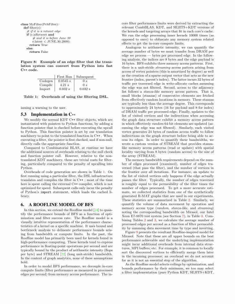
In order to model BFS performance, we decouple in-corecompute limits (filter performance as measured in processededges per second) from memory access performance. The in-

core filter performance limits were derived by extracting therelevant CombBLAS, KDT, and SEJITS+KDT versions ofthe kernels and targeting arrays that fit in each core’s cache.We run the edge processing inner kernels 10000 times (asopposed to once) to obfuscate any memory system relatedeffects to get the in-core compute limits.

Analogous to arithmetic intensity, we can quantify theaverage number of bytes we must transfer from DRAM peredge we process — bytes per processed edge. In the follow-ing analysis, the indices are 8 bytes and the edge payload is16 bytes. BFS exhibits three memory access patterns. First,there is a unit-stride streaming access pattern arising fromaccess of vertex pointers (this is amortized by degree) as wellas the creation of a sparse output vector that acts as the newfrontier (index, parent’s index). The latter incurs 32 bytes oftraffic per traversed edge in write-allocate caches assumingthe edge was not filtered. Second, access to the adjacencylist follows a stanza-like memory access pattern. That is,small blocks (stanzas) of consecutive elements are fetchedfrom effectively random locations in memory. These stanzasare typically less than the average degree. This correspondsto approximately 24 bytes (16 for payload and 8 for index)of DRAM traffic per processed edge. Finally, updates to thelist of visited vertices and the indirections when accessingthe graph data structure exhibit a memory access patternin which effectively random 64-bit elements are updated (as-suming the edge was not filtered). Similarly, each visitedvertex generates 24 bytes of random access traffic to followindirections on the graph structure before being able to ac-cess its edges. In order to quantify these bandwidths, wewrote a custom version of STREAM that provides stanza-like memory access patterns (read or update) with spatiallocality varying from 8 bytes (random access) to the size ofthe array (STREAM).

The memory bandwidth requirements depend on the num-ber of edges processed (examined), number of edges tra-versed (that pass the filter), and the number of vertices inthe frontier over all iterations. For instance, an update tothe list of visited vertices only happens if the edge actuallypasses the filter. Typically, the number of edges traversedis roughly equal to the permeability of the filter times thenumber of edges processed. To get a more accurate esti-mate, we collected statistics from one of the syntheticallygenerated R-MAT graphs that are used in our experiments.These statistics are summarized in Table 2. Similarly, wequantify the volume of data movement by operation andmemory access type (random, stanza-like, and streaming)noting the corresponding bandwidth on Mirasol, our IntelXeon E7-8870 test system (see Section 7), in Table 3. Com-bining Tables 2 and 3, we calculate the average number ofprocessed edges per second as a function of filter permeabil-ity by summing data movement time by type and inverting.

Figure 9 presents the resultant Roofline-inspired model forMirasol. Note that these are all upper bounds on the bestperformance achievable and the underlying implementationmight incur additional overheads from internal data struc-tures, MPI buffers, etc. For example, it is common to locallysort the discovered vertices to efficiently merge them laterin the incoming processor; an overhead we do not accountfor as it is not an essential step of the algorithm.

As the Roofline model selects ceilings by optimization, andbounds performance by their minimum, we too may selecta filter implementation (pure Python KDT, SEJITS+KDT,

Table 2: Statistics about the filtered BFS runs onthe R-MAT graph of Scale 23 (M: million)

Filter Vertices Edges Edgespermeability visited traversed processed

1% 655,904 2.5 M 213 M10% 2,204,599 25.8 M 250 M25% 3,102,515 64.6 M 255 M100% 4,607,907 258 M 258 M

Table 3: Breakdown of the volume of data movementby memory access pattern and operation.

Memory Vertices Edges Edges Bandwidthaccess type visited traversed processed on Mirasol

Random 24 bytes 8 bytes 0 9.09 GB/sStanza 0 0 24 bytes 36.6 GB/sStream 8 bytes 32 bytes 0 106 GB/s

or the CombBLAS limit) and the weighted bandwidth limit(in black) and look for the minimum.

We observe a pure Python KDT filter will result in a per-formance bound more than an order of magnitude lower thanthe bandwidth limit. Conversely, the bandwidth limit isabout 25× lower than the CombBLAS in-core performancelimit. Ultimately, the performance of a SEJITS specializedfilter is sufficiently fast to ensure a BFS implementation willbe bandwidth-bound. This is a very important observationthat explains why SEJITS+KDT performance is so closeto CombBLAS performance in practice (as shown later inSection 7) even though its in-core performance is 4× slower.

7. EXPERIMENTS

7.1 MethodologyTo evaluate our methodology, we examine graph analysis

behavior on an Mirasol, an Intel Nehalem-based machine,as well as the Hopper Cray XE6 supercomputer. Mira-sol is a single node platform composed of four Intel XeonE7-8870 processors. Each socket has ten cores running at2.4 GHz, and supports two-way simultaneous multithread-ing (20 thread contexts per socket). The cores are connectedto a very large 30 MB L3 cache via a ring architecture. Thesustained stream bandwidth is about 30 GB/s per socket.The machine has 256 GB 1067 MHz DDR3 RAM. We useOpenMPI 1.4.3 with GCC C++ compiler version 4.4.5, andPython 2.6.6.

Hopper is a Cray XE6 massively parallel processing (MPP)system, built from dual-socket 12-core “Magny-Cours” Op-teron compute nodes. In reality, each socket (multichipmodule) has two dual hex-core chips, and so a node canbe viewed as a four-chip compute configuration with strongNUMA properties. Each Opteron chip contains six super-scalar, out-of-order cores capable of completing one (dual-slot) SIMD add and one SIMD multiply per cycle. Addi-tionally, each core has private 64 KB L1 and 512 KB low-latency L2 caches. The six cores on a chip share a 6MB L3cache and dual DDR3-1333 memory controllers capable ofproviding an average STREAM [22] bandwidth of 12GB/s

1  

10  

100  

1000  

10000  

100000  

1%   10%   100%  

Millions  of  E

dges  Processed

 per  Secon

d  

Filter  Permeability  

Mirasol  (Xeon  E7  8870,  36  cores)  

Python  KDT  Performance  Bound  

SEJITS+KDT  Performance  Bound  

CombBLAS  Performance  Bound  

DRAM  Performance  Bound  

Figure 9: Roofline-inspired model for filtered BFScomputations. Performance bounds arise frombandwidth, CombBLAS, KDT, or SEJITS+KDT fil-ter performance, and filter success rate.

!

"

#

$

%&''&()*+,+-./0,

!

"

#

$

123(224*+,+-./0,

"

#

$

5(2236)*78927,9&:;)*27,+-./0,! =

Figure 10: Toy example illustrating the process ofbuilding a combined graph induces by the tweets

per chip. Each pair of compute nodes shares one Gemininetwork chip, which collectively form a 3D torus. We useCray’s MPI implementation, which is based on MPICH2,and compile our code with GCC C++ compiler version 4.6.2and Python 2.7. Complicating our experiments, some com-pute nodes do not contain a compiler; we ensured that acompute node with compilers available was used to buildthe SEJITS+KDT filters.

7.2 Test data setsFor most of our parallel scaling studies, we use synthetically-

generated R-MAT [18] graphs with a very skewed degreedistribution. An R-MAT graph of scale N has 2N verticesand approximately edgefactor ∗ 2N edges. In our tests, ouredgefactor is 16, and our R-MAT seed paratemeters a, b, c,and d are 0.59, 0.19, 0.19, 0.05 respectively. After generatingthis non-semantic (boolean) graph, the edge payloads areartificially introduced using a random number generator ina way that ensures targer filter permeability. The edge typeis the same as the Twitter edge type described below, to beconsistent between experiments on real and synthetic data.

We also use graphs from real social network interactions,from anonymized Twitter data. In our Twitter graphs, edgescan represent two different types of interactions. The first

struct TwitterEdge{

bool follower;time t latest; // set if count>0short count; // number of tweets

};

Figure 11: The edge data structure used forthe tweet-induced combined (tweeting+following)graph in C++ (methods are omitted for brevity)

Table 4: Sizes (vertex and edge counts) of differentcombined twitter graphs.

LabelVertices Edges (millions)

(millions) Tweet Follow Tweet&followSmall 0.5 0.7 65.3 0.3

Medium 4.2 14.2 386.5 4.8Large 11.3 59.7 589.1 12.5Huge 16.8 102.4 634.2 15.6

interaction is the“following”relationship where an edge fromvi to vj means that vi is following vj (note that these direc-tions are consistent with the common authority-hub defini-tions in the World Wide Web). The second interaction en-codes an abbreviated “retweet” relationship: an edge fromvi to vj means that vi has mentioned vj at least once intheir tweets. The edge also keeps the number of such tweets(count) as well as the last tweet date if count is larger thanone.

The tweets occurred in the period of June-December of2009. To allow scaling studies, we creates subsets of thesetweets, based on the date they occur. The small datasetcontains tweets from the first two weeks of June, the mediumdataset contains tweets that happened in June and July,the large dataset contains tweets dated June-September, andfinally the huge dataset contains all the tweets from June toDecember.

These partial tweets are then induced upon the graphthat represents the follower/followee relationship. If a per-son tweeted someone or has been tweeted by someone, thenthe vertex is retained in the tweet-induced combined graph.

!"#$

%"!$

&"!$

'"!$

("!$

%)"!$

*&"!$

%+$ %!+$ &#+$ %!!+$

!"#$%&'

(%)*

"%

'+,-".%/".*"#0+,+-1%

,-.$/0123451657389$ ,-.$ :;<=.:>,-.$ ?@0ABCD:$

Figure 12: Relative breadth-first search perfor-mance of four methods. y-axis uses a log scale.The experiments are run using 24 nodes of Hopper,where each node has two 12-code AMD processors.

Table 5: Statistics about the largest strongly con-nected components of the twitter graphs

Vertices Edges traversed Edges processedSmall 78,397 147,873 29.4 million

Medium 55,872 93,601 54.1 millionLarge 45,291 73,031 59.7 millionHuge 43,027 68,751 60.2 million

!"#$%!"&'%!"'!%#"!!%&"!!%("!!%)"!!%#*"!!%$&"!!%*("!!%#&)"!!%

+,-..% ,/012,% .-34/%% 524/%

!"#$%&'

(%)*

"%

+,-."/%-$012%3/#04%

678%9,-:/31-.1;/0<% 678% =>?@8=A678% BC,DEFG=%

Figure 13: Relative filtered breadth-first search per-formance of four methods on real Twitter data. They-axis is in seconds on a log scale. The runs use 36cores (4 sockets) of Intel Xeon E7-8870 processors.

A simple example shows this process in Figure 10. Node 1is eliminated because it has not tweeted about anyone, norhas it been tweeted by someone. All the follower/followeeedges connected to Node 1 are also eliminated. In the com-bined graph, three edges remain: e(2, 3), e(2, 4), and e(4, 3).Each edge can potentially encode both the following relationand the tweeted relationship, however both fields are neededonly in the case of e(4, 3). The data structure for edges inthe combined graph is shown in Figure 11.

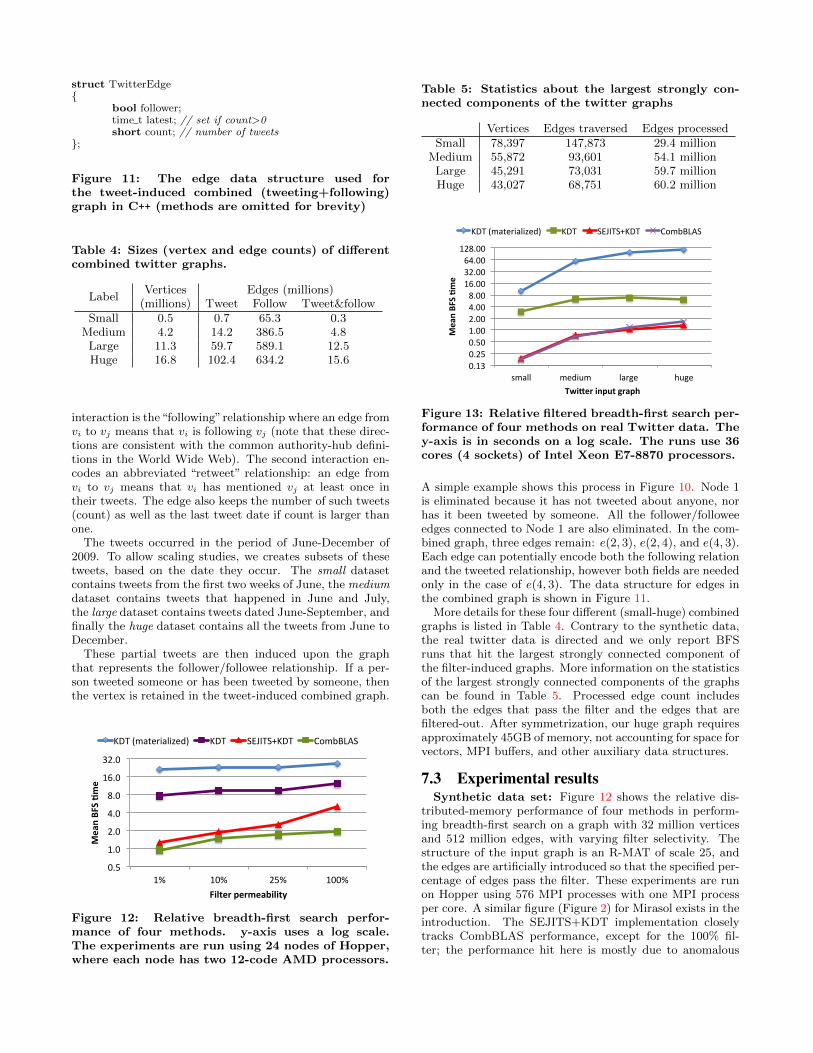
More details for these four different (small-huge) combinedgraphs is listed in Table 4. Contrary to the synthetic data,the real twitter data is directed and we only report BFSruns that hit the largest strongly connected component ofthe filter-induced graphs. More information on the statisticsof the largest strongly connected components of the graphscan be found in Table 5. Processed edge count includesboth the edges that pass the filter and the edges that arefiltered-out. After symmetrization, our huge graph requiresapproximately 45GB of memory, not accounting for space forvectors, MPI buffers, and other auxiliary data structures.

7.3 Experimental resultsSynthetic data set: Figure 12 shows the relative dis-

tributed-memory performance of four methods in perform-ing breadth-first search on a graph with 32 million verticesand 512 million edges, with varying filter selectivity. Thestructure of the input graph is an R-MAT of scale 25, andthe edges are artificially introduced so that the specified per-centage of edges pass the filter. These experiments are runon Hopper using 576 MPI processes with one MPI processper core. A similar figure (Figure 2) for Mirasol exists in theintroduction. The SEJITS+KDT implementation closelytracks CombBLAS performance, except for the 100% fil-ter; the performance hit here is mostly due to anomalous

!"!#$!"!%$!"&#$!"'($!"(!$&"!!$'"!!$)"!!$*"!!$&%"!!$

+,-..$ ,/012,$ .-34/$$ 524/$

!"#$%&'

(%)*

"%

+,-."/%-$012%3/#04%

678$9,-:/31-.1;/0<$ 678$ =>?@8=A678$ BC,DEFG=$

Figure 14: Relative filtered breadth-first search per-formance of four methods on real twitter data; y-axisis in seconds on a log scale. The experiments are runusing 24 nodes of Hopper, where each node has two12-code AMD processors.

performance variability on the test machine.Twitter data set: The filter used in the experiments

with the Twitter data set is to keep edges whose latestretweeting interaction happened by June 30, 2009, and isexplained in detail in Section 1.3. Figure 13 shows the rela-tive performance of four systems in performing breadth-firstsearch on real graphs that represent the twitter interactiondata on Mirasol. Figure 14 shows the same graph Hopperusing 576 MPI processes. SEJIT+KDT’s performance isidentical to the performance of CombBLAS in these datasets, showing that for real-life inspired cases, our approachis as fast as the underlying high-performance library.

Parallel scaling: The parallel scaling of our approachis shown in Figure 15 for lower concurrencies on Mirasol.CombBLAS achieves remarkable linear scaling with increas-ing process counts (34-36X on 36 cores), while SEJITS+KDTclosely tracks its performance and scaling. Single core KDTruns did not finish in a reasonable time to report. We donot report performance of materialized filters as they werepreviously shown to be the slowest.

Parallel scaling at higher concurrencies is done on Hop-per, using the scale 25 synthetic R-MAT data set. Figure 16shows the comparative performance of KDT on-the-fly fil-ters, SEJITS+KDT, and CombBLAS, with 10% and 25%filter permeability.

Finally, we show weak scaling results on Hopper using 1%filter permeability (other cases experienced similar perfor-mance). In this run, shown in Figure 17, each MPI processis responsible for approximately 11 million original edges(hence 22 million edges after symmetricization). More con-cretely, 121-concurrency runs are obtained on a scale 23R-MAT graph, 576-concurrency runs are obtained on scale25 R-MAT graph, and 2025-concurrency runs are obtainedon scale 27 R-MAT graph (1 billion edges). KDT curve ismostly flat (only 9% deviation) due to its in-core compu-tational bottlenecks, while SEJITS+KDT and CombBLASshows higher deviations (54% and 62%, respectively) fromthe perfect flat line. However, these deviations are expectedon a large scale BFS run and experienced on similar archi-tectures [6].

8. CONCLUSIONThe KDT graph analytics system achieves customizability

through user-defined filters, high performance through theuse of a scalable parallel library, and conceptual simplicity

!"#"$"%"!&"'#"&$"

!#%"#(&"

!" #" $" %" !&" '#" &$"

!"#$%&'

(%)*

"%

+,*-".%/0%!12%3./4"55"5%

)*+" ,-./+,0)*+" 1234567,"

(a) 1% permeable

!"

#"

$"

%&"

'!"

&#"

%!$"

!(&"

%" !" #" $" %&" '!" &#"

!"#$%&'

(%)*

"%

+,*-".%/0%!12%3./4"55"5%

)*+" ,-./+,0)*+" 1234567,"

(b) 10% permeable

!"#"$"%"!&"'#"&$"

!#%"#(&"

!" #" $" %" !&" '#" &$"

!"#$%&'

(%)*

"%

+,*-".%/0%!12%3./4"55"5%

)*+" ,-./+,0)*+" 1234567,"

(c) 25% permeable

!"

#"

$"

%&"

'!"

&#"

%!$"

!(&"

%" !" #" $" %&" '!" &#"

!"#$%&'

(%)*

"%

+,*-".%/0%!12%3./4"55"5%

)*+" ,-./+,0)*+" 1234567,"

(d) 100% permeable

Figure 15: Parallel ‘strong scaling’ results of filteredBFS on Mirasol, with varying filter permeability ona synthetic data set (R-MAT scale 23). Both axesare in log-scale, time is in seconds.

!"#$%!"$!%&"!!%#"!!%'"!!%("!!%&)"!!%*#"!!%)'"!!%

&#&% #$)% $+)% &!#'% #!#$%

!"#$%&'

(%)*

"%

+,*-".%/0%!12%3./4"55"5%

,-.% /012./3,-.% 456789:/%

(a) 10% permeable

!"#$%!"$!%&"!!%#"!!%'"!!%("!!%&)"!!%*#"!!%)'"!!%

&#&% #$)% $+)% &!#'% #!#$%

!"#$%&'

(%)*

"%

+,*-".%/0%!12%3./4"55"5%

,-.% /012./3,-.% 456789:/%

(b) 25% permeable

Figure 16: Parallel ‘strong scaling’ results of filteredBFS on Hopper, with varying filter permeability ona synthetic data set (R-MAT scale 25). Both axesare in log-scale, time is in seconds.

through appropriate graph abstractions expressed in a high-level language.

We have shown that the performance hit of expressingfilters in a high-level language can be mitigated by Just-in-Time Specialization. In particular, we have shown that ourembedded DSL for filters can enable Python code to achievecomparable performance to a pure C++ implementation. Aroofline analysis shows that the specializer enables filteringto move from being compute-bound to memory bandwidth-bound. We demonstrated our approach on both real-worlddata and large generated datasets. Our approach scales tographs on the order of hundreds of millions of edges, andmachines with thousands of processors.

In future work we will further generalize our DSL to sup-port a larger subset of Python, as well as expand SEJITSsupport beyond filtering to cover more KDT primitives. Anopen question is whether CombBLAS performance can bepushed closer to the bandwidth limit by eliminating inter-nal data structure overheads.

AcknowlegementsThis work was supported in part by National Science Foun-dation grant CNS-0709385. Portions of this work were per-formed at the UC Berkeley Parallel Computing Laboratory

!"#$

%"!$

&"!$

'"!$

("!$

%)"!$

%&%$ #*)$ &!&#$

!"#$%&'

(%)*

"%

+,*-".%/0%!12%3./4"55"5%

+,-$ ./01-.2+,-$ 3456789.$

Figure 17: Parallel ‘weak scaling’ results of filteredBFS on Hopper, using 1% percent permeability. y-axis is in log scale, time is in seconds.

(Par Lab), supported by DARPA (contract #FA8750-10-1-0191) and by the Universal Parallel Computing ResearchCenters (UPCRC) awards from Microsoft Corp. (Award#024263) and Intel Corp. (Award #024894), with matchingfunds from the UC Discovery Grant (#DIG07-10227) andadditional support from Par Lab affiliates National Instru-ments, NEC, Nokia, NVIDIA, Oracle, and Samsung. Thisresearch used resources of the National Energy Research Sci-entific Computing Center, which is supported by the Officeof Science of the U.S. Department of Energy under ContractNo. DE-AC02-05-CH-11231. Authors from Lawrence Berke-ley National Laboratory were supported by the DOE Officeof Advanced Scientific Computing Research under contractnumber DE-AC02-05-CH-11231.

9. REFERENCES[1] Active Record - Object-Relation Mapping Put on

Rails. http://ar.rubyonrails.org, 2012.

[2] Knowledge Discovery Toolbox.http://kdt.sourceforge.net, 2012.

[3] D. A. Bader and K. Madduri. SNAP, small-worldnetwork analysis and partitioning: An open-sourceparallel graph framework for the exploration oflarge-scale networks. In IPDPS’08: Proceedings of the2008 IEEE International Symposium onParallel&Distributed Processing, pages 1–12. IEEEComputer Society, 2008.

[4] J.W. Berry, B. Hendrickson, S. Kahan, andP. Konecny. Software and Algorithms for GraphQueries on Multithreaded Architectures. In Proc.Workshop on Multithreaded Architectures andApplications. IEEE Press, 2007.

[5] A. Buluc and J.R. Gilbert. The Combinatorial BLAS:Design, implementation, and applications.International Journal of High Performance ComputingApplications (IJHPCA), 25(4):496–509, 2011.

[6] A. Buluc and K. Madduri. Parallel breadth-firstsearch on distributed memory systems. In Proc.Supercomputing, 2011.

[7] B. Catanzaro, S.A. Kamil, Y. Lee, K. Asanovic,J. Demmel, K. Keutzer, J. Shalf, K.A. Yelick, andA. Fox. SEJITS: Getting Productivity andPerformance With Selective Embedded JIT

Specialization. In Workshop on Programming Modelsfor Emerging Architectures (PMEA), 2009.

[8] Timothy A. Davis. Direct Methods for Sparse LinearSystems (Fundamentals of Algorithms 2). Society forIndustrial and Applied Mathematics, Philadelphia,PA, USA, 2006.

[9] J. Dean and S. Ghemawat. MapReduce: simplifieddata processing on large clusters. In Proc. 6thSymposium on Operating System Design andImplementation, pages 137–149, Berkeley, CA, USA,2004. USENIX Association.

[10] Martin Fowler. Domain Specific Languages.Addison-Wesley Professional, 2010.

[11] J.R. Gilbert, C. Moler, and R. Schreiber. Sparsematrices in MATLAB: Design and implementation.SIAM J. Matrix Anal. Appl, 13:333–356, 1992.

[12] D. Gregor and A. Lumsdaine. The Parallel BGL: AGeneric Library for Distributed Graph Computations.In Proc. Workshop on Parallel/High-PerformanceObject-Oriented Scientific Computing (POOSC’05),2005.

[13] S. Hong, H. Chafi, E. Sedlar, and K. Olukotun.Green-Marl: a DSL for easy and efficient graphanalysis. In Proceedings of the seventeenthinternational conference on Architectural Support forProgramming Languages and Operating Systems,ASPLOS ’12, pages 349–362, New York, NY, USA,2012. ACM.

[14] S. Kamil, D. Coetzee, S. Beamer, H. Cook, E. Gonina,J. Harper, J. Morlan, and A. Fox. Portable parallelperformance from sequential, productive, embeddeddomain specific languages. In Proceedings of the ACMSIGPLAN Symposium on Principles and Practices ofParallel Programming, 2012.

[15] U. Kang, C.E. Tsourakakis, and C. Faloutsos.PEGASUS: A Peta-Scale Graph Mining System -Implementation and Observations. In Data Mining,2009. ICDM’09. Ninth IEEE International Conferenceon, pages 229–238. IEEE, 2009.

[16] Ora Lassila and Ralph R. Swick. Resource DescriptionFramework (RDF) Model and Syntax Specification.W3c recommendation, W3C, February 1999.

[17] Daan Leijen and Erik Meijer. Domain specificembedded compilers. In Proceedings of the 2ndconference on Conference on Domain-SpecificLanguages - Volume 2, DSL’99, pages 9–9, Berkeley,CA, USA, 1999. USENIX Association.

[18] J. Leskovec, D. Chakrabarti, J. Kleinberg, andC. Faloutsos. Realistic, Mathematically TractableGraph Generation and Evolution, Using KroneckerMultiplication. In PKDD, pages 133–145. Springer,2005.

[19] A. Lugowski, D. Alber, A. Buluc, J. Gilbert,S. Reinhardt, Y. Teng, and A. Waranis. A FlexibleOpen-Source Toolbox for Scalable Complex GraphAnalysis. In Proceedings of the Twelfth SIAMInternational Conference on Data Mining (SDM12),pages 930–941, April 2012.

[20] A. Lugowski, A. Buluc, J. Gilbert, and S. Reinhardt.Scalable Complex Graph Analysis with the KnowledgeDiscovery Toolbox. In International Conference onAcoustics, Speech, and Signal Processing (ICASSP),

2012.

[21] G. Malewicz, M.H. Austern, A.J.C. Bik, J.C. Dehnert,I. Horn, N. Leiser, and G. Czajkowski. Pregel: ASystem for Large-Scale Graph Processing. InProceedings of the 2010 International Conference onManagement of Data, SIGMOD ’10, pages 135–146,New York, NY, USA, 2010. ACM.

[22] J. D. McCalpin. STREAM: Sustainable MemoryBandwidth in High Performance Computers.http://www.cs.virginia.edu/stream/.

[23] Eric Prud’hommeaux and Andy Seaborne. SPARQLquery language for RDF (working draft). Technicalreport, W3C, March 2007.

[24] S. Williams, A. Waterman, and D. Patterson.Roofline: an insightful visual performance model formulticore architectures. Communications of the ACM,52(4):65–76, 2009.