graph cut based inference with co-occurrence statisticslubor/eccv10co.pdf · graph cut based...

Graph Cut based Inference with Co-occurrenceStatistics

Lubor Ladicky1,3, Chris Russell1,3, Pushmeet Kohli2, and Philip H.S. Torr1

1 Oxford Brookes2 Microsoft Research

Abstract. Markov and Conditional random fields (CRFs) used in computer vi-sion typically model only local interactions between variables, as this is compu-tationally tractable. In this paper we consider a class of global potentials definedover all variables in the CRF. We show how they can be readily optimised us-ing standard graph cut algorithms at little extra expense compared to a standardpairwise field.This result can be directly used for the problem of class based image segmenta-tion which has seen increasing recent interest within computer vision. Here theaim is to assign a label to each pixel of a given image from a set of possible ob-ject classes. Typically these methods use random fields to model local interactionsbetween pixels or super-pixels. One of the cues that helps recognition is globalobject co-occurrence statistics, a measure of which classes (such as chair or mo-torbike) are likely to occur in the same image together. There have been severalapproaches proposed to exploit this property, but all of them suffer from differentlimitations and typically carry a high computational cost, preventing their ap-plication on large images. We find that the new model we propose produces animprovement in the labelling compared to just using a pairwise model.

1 Introduction

Class based image segmentation is a highly active area of computer vision researchas is shown by a spate of recent publications [11,22,29,31,34]. In this problem, everypixel of the image is assigned a choice of object class label, such as grass, person, ordining table. Formulating this problem as a likelihood, in order to perform inference, is adifficult problem, as the cost or energy associated with any labelling of the image shouldtake into account a variety of cues at different scales. A good labelling should takeaccount of: low-level cues such as colour or texture [29], that govern the labelling ofsingle pixels; mid-level cues such as region continuity, symmetry [23] or shape [2] thatgovern the assignment of regions within the image; and high-level statistics that encodeinter-object relationships, such as which objects can occur together in a scene. Thiscombination of cues makes for a multi-scale cost function that is difficult to optimise.

3 The authors assert equal contribution and joint first authorshipThis work was supported by EPSRC, HMGCC and the PASCAL2 Network of Excellence.Professor Torr is in receipt of a Royal Society Wolfson Research Merit Award.

2 Lubor Ladicky, Chris Russell, Pushmeet Kohli, and Philip H.S. Torr

Current state of the art low-level approaches typically follow the methodology pro-posed in Texton-boost [29], in which weakly predictive features such as colour, location,and texton response are used to learn a classifier which provides costs for a single pixeltaking a particular label. These costs are combined in a contrast sensitive ConditionalRandom Field CRF [19].

The majority of mid-level inference schemes [25,20] do not consider pixels directly,rather they assume that the image has been segmented into super-pixels [5,8,28]. Alabelling problem is then defined over the set of regions. A significant disadvantageof such approaches is that mistakes in the initial over-segmentation, in which regionsspan multiple object classes, cannot be recovered from. To overcome this [10] proposeda method of reshaping super-pixels to recover from the errors, while the work [17]proposed a novel hierarchical framework which allowed for the integration of multipleregion-based CRFs with a low-level pixel based CRF, and the elimination of inconsistentregions.

These approaches can be improved by the inclusion of costs based on high levelstatistics, including object class co-occurrence, which capture knowledge of scene se-mantics that humans often take for granted: for example the knowledge that cows andsheep are not kept together and less likely to appear in the same image; or that mo-torbikes are unlikely to occur near televisions. In this paper we consider object classco-occurrence to be a measure of how likely it is for a given set of object classes tooccur together in an image. They can also be used to encode scene specific informationsuch as the facts that computer monitors and stationary are more likely to occur in of-fices, or that trees and grass occur outside. The use of such costs can help prevent someof the most glaring failures in object class segmentation, such as the labelling of a cowas half cow and half sheep, or the mistaken labelling of a boat surrounded by water as abook.

As well as penalising strange combinations of objects appearing in an image, co-occurrence potentials can also be used to impose an MDL1 prior that encourages aparsimonious description of an image using fewer labels. As discussed eloquently in therecent work [4], the need for a bias towards parsimony becomes increasingly importantas the number of classes to be considered increases.

Figure 1 illustrates the importance of co-occurrence statistics in image labelling.The promise of co-occurrence statistics has not been ignored by the vision commu-

nity. In [22] Rabinovich et al. proposed the integration of such co-occurrence costs thatcharacterise the relationship between two classes. Similarly Torralba et al. [31] pro-posed scene-based costs that penalised the existence of particular classes in a contextdependent manner. We shall discuss these approaches, and some problems with them inthe next section.

2 CRFs and Co-occurrence

A conventional CRF is defined over a set of random variables V = {1, 2, 3, . . . , n}where each variable takes a value from the label set L = {l1, l2, . . . , lk} corresponding

1 Minimum description length

Graph Cut based Inference with Co-occurrence Statistics 3

(a) (b) (c) (a) (b) (c)

Fig. 1. Best viewed in colour: Qualitative results of object co-occurrence statistics. (a) Typical images taken from theMSRC data set [29]; (b) A labelling based upon a pixel based random field model [17] that does not take into accountco-occurrence; (c) A labelling of the same model using co-occurrence statistics. The use of co-occurrence statistics to guidethe segmentation results in a labelling that is more parsimonious and more likely to be correct. These co-occurrence statisticssuppress the appearance of small unexpected classes in the labelling. Top left: a mistaken hypothesis of a cow is suppressedTop right: Many small classes are suppressed in the image of a building. Note that the use of co-occurrence typically changeslabels, but does not alter silhouettes.

to the set of object classes. An assignment of labels to the set of random variables willbe referred to as a labelling, and denoted as x ∈ L|V|. We define a cost function E(x)over the CRF of the form:

E(x) =∑c∈C

ψc(xc) (1)

where the potential ψc is a cost function defined over a set of variables (called a clique)c, and xc is the state of the set of random variables that lie within c. The set C of cliquesis a subset of the power set of V , i.e. C ⊆ P (V). In the majority of vision problems, thepotentials are defined over a clique of size at most 2. Unary potentials are defined over aclique of size one, and typically based upon classifier responses (such as ada-boost [29]or kernel SVMs [27]), while pairwise potentials are defined over cliques of size two andmodel the correlation between pairs of random variables.

2.1 Incorporating Co-occurrence Potentials

To model object class co-occurrence statistics a new term K(x) is added to the energy:

E(x) =∑

ψc(xc) +K(x). (2)

The question naturally arises as to what form an energy involving co-occurrence termsshould take. We now list a set of desiderata that we believe are intuitive for any co-occurrence cost.

(i) Global Energy: We would like a formulation of co-occurrence that allows usto estimate the segmentation using all the data directly, by minimising a single costfunction of the form (2). Rather than any sort of two stage process in which a harddecision is made of which objects are present in the scene a priori as in [31].

(ii) Invariance: The co-occurrence cost should depend only on the labels presentin an image, it should be invariant to the number and location of pixels that object


occupies. To reuse an example from [32], the surprise at seeing a polar bear in a streetscene should not not vary with the number of pixels that represent the bear in the image.

(iii) Efficiency: Inference should be tractable, i.e. the use of co-occurrence shouldnot be the bottle-neck preventing inference. As the memory requirements of any con-ventional inference algorithm [30] is typically O(|V|) for vision problems, the memoryrequirements of a formulation incorporating co-occurrence potentials should also beO(|V|).

(iv) Parsimony: The cost should follow the principle of parsimony in the followingway: if several solutions are almost equally likely then the solution that can describethe image using the fewest distinct labels should be chosen. Whilst this might not seemimportant when classifying pixels into a few classes, as the set of putative labels foran image increases the chance of speckle noise due to misclassification will increaseunless a parsimonious solution is encouraged.

While these properties seem uncontroversial, no prior work exhibits property (ii).Similarly, no approaches satisfy properties (i) and (iii) simultaneously. In order to sat-isfy condition (ii) the co-occurrence cost K(x) defined over x must be a function de-fined on the set of labels L(x) = {l ∈ L : ∃xi = l} present in the labelling x; thisguarantees invariance to the size of an object:

K(x) = C(L(x)) (3)

Embedding the co-occurrence term in the CRF cost function (1), we have:

E(x) =∑c∈C

ψc(xc) + C(L(x)). (4)

To satisfy the parsimony condition (iv) potentials must act to penalise the unex-pected appearance of combinations of labels in a labelling. This observation can beformalised as the statement that the cost C(L) monotonically increasing with respectto the label set L i.e. :

L1 ⊂ L2 =⇒ C(L1) ≤ C(L2). (5)

The new potential C(L(x)) can be seen as a particular higher order potential definedover a clique which includes the whole of V , i.e. ψV (x).

2.2 Prior Work

There are two existing approaches to co-occurrence potentials, neither of which usespotentials defined over a clique of size greater than two. The first makes an initial hardestimate of the type of scene, and updates the unary potentials associated with eachpixel to encourage or discourage particular choices of label, on the basis of how likelythey are to occur in the scene. The second approach models object co-occurrence as apairwise potential between regions of the image.

Torralba et al. [31] proposed the use of additional unary potentials to capture scenebased occurrence priors. Their costs took the form:

K(x) =∑i∈V

φ(xi). (6)


While the complexity of inference over such potentials scales linearly with the size ofthe graph, they are prone to over counting costs, violating (ii), and require an initialhard decision of scene type before inference, which violates (i). As it encourages theappearance of all labels which are common to a scene, it does not necessarily encourageparsimony (iv).

A similar approach was seen in the Pascal VOC2008 object segmentation challenge,where the best performing method, by Csurka [6], worked in two stages. Initially theset of object labels present in the image was estimated, and in the second stage, a labelfrom the estimated label set was assigned to each image pixel. As no cost functionK(·)was proposed, it is open to debate if it satisfied (ii) or (iv).

MethodGlobal energy

(i)Invariance

(ii)Efficiency

(iii)Parsimony

(iv)

Unary [31] 7 7 3 7Pairwise [22,9,32] 3 7 7 3Csurka [6] 7 — 3 —Our approach 3 3 3 3

Fig. 2. A comparison of the capabilities of existing image co-occurrence formulations against ournew approach. See section 2.2 for details.

Rabinovich et al. [9,22], and independently [32], proposed co-occurrence as a softconstraint that approximated C(L(x)) as a pairwise cost defined over a fully connectedgraph that took the form:

K(x) =∑i,j∈V

φ(xi, xj), (7)

where φ was some potential which penalised labels that should not occur together inan image. Unlike our model (4) the penalty cost for the presence of pairs of labels, thatrarely occur together, appearing in the same image grows with the number of randomvariables taking these labels, violating assumption (ii). While this serves as a functionalpenalty that prevents the occurrence of many classes in the same labelling, it does notaccurately model the co-occurrence costs we described earlier. The memory require-ments of inference scales badly with the size of a fully connected graph. It grows withcomplexity O(|V|2) rather than O(|V|) with the size of the graph, violating constraint(iii). Providing the pairwise potentials are semi-metric [3], it does satisfy the parsimonycondition (iv).

To minimise these difficulties, previous approaches defined variables over segmentsrather than pixels. Such segment based methods work under the assumption that somesegments share boundaries with objects in the image. This is not always the case, andthis assumption may result in dramatic errors in the labelling. The relationship betweenprevious approaches and the desiderata can be seen in figure 2.


Two efficient schemes [7,12] have been proposed for the minimisation of the num-ber of classes or objects present in a scene. While neither of them directly models classbased co-occurrence relationships, their optimisation approaches do satisfy our desider-ata.

One such approach was proposed by Hoiem et al. [12], who used a cost based onthe number of objects in the scene, in which the presence of any instance of any objectincurs a uniform penalty cost. For example, the presence of both a motorbike and a busin a single image is penalised as much as the presence of two buses. Minimising thenumber of objects in a scene is a good method of encouraging consistent labellings, butdoes not capture any co-occurrence relationship between object classes.

In a recent work, appearing at the same time as ours, Delong et al. [7] proposed theuse of a soft cost over the number of labels present in an image for clustering. While themathematical formulation they propose is more flexible than this, they do not suggestany applications of this increased flexibility. Moreover, their formulation is less generalthan ours as it does not support the full range of monotonically increasing label setcosts.

3 Inference on global co-occurrence potentials

Consider the energy (4) defined in section 2.1. The inference problem becomes:

x∗ = arg minx∈L|V|∑c∈C ψc(xc) + C(L(x))

s.t. x ∈ L|V|, L(x) = {l ∈ L : ∃xi = l}. (8)

In the general case the problem of minimising this energy can be reformulated as an in-teger program and approximately solved as an LP-relaxation [16]. This LP-formulationcan be transformed using a Lagrangian relaxation into a pairwise energy, allowing al-gorithms, such as Belief Propagation [33] or TRW-S [14], that can minimise arbitrarypairwise energies to be applied [16]. However, reparameterisation methods such asthese perform badly on densely connected graphs [15,26].

In this section we show that under assumption, that C(L) is monotonically increas-ing with respect to L, the problem can be solved efficiently using αβ-swap and α-expansion moves [3], where the number of additional edges of the graph grows linearlywith the number of variables in the graph. In contrast to [22], these algorithms can beapplied to large graphs with more than 200, 000 variables.

Move making algorithms project the problem into a smaller subspace in which asub-problem is efficiently solvable. Solving this sub-problem proposes optimal moveswhich guarantee that the energy decreases after each move and must eventually con-verge. The performance of move making algorithms depends dramatically on the sizeof the move space. The expansion and swap move algorithms we consider project theproblem into two label sub-problem and under the assumption that the projected energyis pairwise and submodular, it can be solved using graph cuts. Because the energy (4)is additive, we derive graph constructions only for term C(L(x)). Both the applicationof swap and expansion moves to minimise the energy, and the graph construction forthe other terms proceed as described in [3].


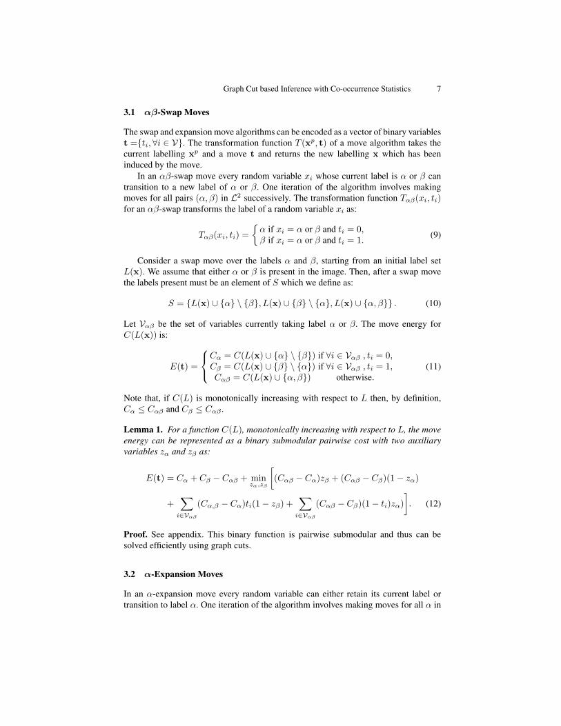
3.1 αβ-Swap Moves

The swap and expansion move algorithms can be encoded as a vector of binary variablest ={ti,∀i ∈ V}. The transformation function T (xp, t) of a move algorithm takes thecurrent labelling xp and a move t and returns the new labelling x which has beeninduced by the move.

In an αβ-swap move every random variable xi whose current label is α or β cantransition to a new label of α or β. One iteration of the algorithm involves makingmoves for all pairs (α, β) in L2 successively. The transformation function Tαβ(xi, ti)for an αβ-swap transforms the label of a random variable xi as:

Tαβ(xi, ti) ={α if xi = α or β and ti = 0,β if xi = α or β and ti = 1. (9)

Consider a swap move over the labels α and β, starting from an initial label setL(x). We assume that either α or β is present in the image. Then, after a swap movethe labels present must be an element of S which we define as:

S = {L(x) ∪ {α} \ {β}, L(x) ∪ {β} \ {α}, L(x) ∪ {α, β}} . (10)

Let Vαβ be the set of variables currently taking label α or β. The move energy forC(L(x)) is:

E(t) =

Cα = C(L(x) ∪ {α} \ {β}) if ∀i ∈ Vαβ , ti = 0,Cβ = C(L(x) ∪ {β} \ {α}) if ∀i ∈ Vαβ , ti = 1,Cαβ = C(L(x) ∪ {α, β}) otherwise.

(11)

Note that, if C(L) is monotonically increasing with respect to L then, by definition,Cα ≤ Cαβ and Cβ ≤ Cαβ .

Lemma 1. For a function C(L), monotonically increasing with respect to L, the moveenergy can be represented as a binary submodular pairwise cost with two auxiliaryvariables zα and zβ as:

E(t) = Cα + Cβ − Cαβ + minzα,zβ

[(Cαβ − Cα)zβ + (Cαβ − Cβ)(1− zα)

+∑i∈Vαβ

(Cα,β − Cα)ti(1− zβ) +∑i∈Vαβ

(Cαβ − Cβ)(1− ti)zα)]. (12)

Proof. See appendix. This binary function is pairwise submodular and thus can besolved efficiently using graph cuts.

3.2 α-Expansion Moves

In an α-expansion move every random variable can either retain its current label ortransition to label α. One iteration of the algorithm involves making moves for all α in


L successively. The transformation function Tα(xi, ti) for an α-expansion move trans-forms the label of a random variable xi as:

Tα(xi, ti) ={α if ti = 0xi if ti = 1. (13)

To derive a graph-construction that approximates the true cost of an α-expansion movewe rewrite C(L) as:

C(L) =∑B⊆L

kB , (14)

where the coefficients kB are calculated recursively as:

kB = C(B)−∑B′⊂B

kB′ . (15)

As a simplifying assumption, let us first assume there is no variable currently takinglabel α. Let A be set of labels currently present in the image and δl(t) be set to 1 iflabel l is present in the image after the move and 0 otherwise. Then:

δα(t) ={

1 if ∃i ∈ V s.t. ti = 0,0 otherwise. (16)

∀l ∈ A , δl(t) ={

1 if ∃i ∈ Vl s.t. ti = 1,0 otherwise. (17)

The α-expansion move energy of C(L(x)) can be written as:

E(t) = Enew(t)− Eold =∑

B⊆A∪{α}

kB∏l∈B

δl(t)− C(A).

Ignoring the constant term and decomposing the sum into parts with and without termsdependent on α we have:

E(t) =∑B⊆A

kB∏l∈B

δl(t) +∑B⊆A

kB∪{α}δα(t)∏l∈B

δl(t). (18)

As either α or all subsets B ⊆ A are present after any move, the following statementholds:

δα(t)∏l∈B

δl(t) = δα(t) +∏l∈B

δl(t)− 1. (19)

Replacing the term δα(t)∏l∈B δl(t) and disregarding new constant terms, equation

(18) becomes:

E(t) =∑B⊆A

kB∪{α}δα(t)+∑B⊆A

(kB+kB∪{α})∏l∈B

δl(t) = k′αδα(t)+∑B⊆A

k′B∏l∈B

δl(t),

(20)where k′α =

∑B⊆A kB∪{α} = C(B ∪ {α})− C(B) and k′B = kB + kB∪{α}.


E(t) is, in general, a higher-order non-submodular energy, and intractable. How-ever, when proposing moves we can use the procedure described in [21,24] and over-estimate second term K(A, t) =

∑B⊆A k

′B

∏l∈B δl(t) of the cost of moving from the

current solution.For any l′ ∈ A we can overestimate K(A, t) by

K(A, t) ≤ K(A \ {l′}, t) + δl′(t) minS⊆A\{l′}

∑B⊆S

(k′B∪{l′} − k′B)

= K(A \ {l′}, t) + k′′l′δl′(t), (21)

where k′′(l′) is always non-negative for all C(L) that are monotonically increasingwith respect to L. By applying this decomposition iteratively for any ordering of labelsl′ ∈ A we obtain :

K(A, t) ≤ K +∑l∈A

k′′l δl(t). (22)

The constant term K can be ignored, because it does not affect the optimality of themove. Heuristically we pick l′ in each iteration as

l′ = arg minl∈A

minS⊆A\{l}

∑B⊆S

(k′B∪{l} − k′B). (23)

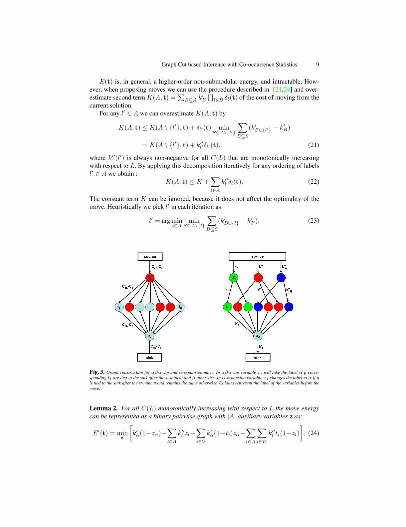
Fig. 3. Graph construction for αβ-swap and α-expansion move. In αβ-swap variable xi will take the label α if corre-sponding ti are tied to the sink after the st-mincut and β otherwise. In α-expansion variable xi changes the label to α if itis tied to the sink after the st-mincut and remains the same otherwise. Colours represent the label of the variables before themove.

Lemma 2. For all C(L) monotonically increasing with respect to L the move energycan be represented as a binary pairwise graph with |A| auxiliary variables z as:

E′(t) = minz

[k′α(1−zα)+

∑l∈A

k′′l zl+∑i∈V

k′α(1−ti)zα+∑l∈A

∑i∈Vl

k′′l ti(1−zl)], (24)


(a) (b) (c) (a) (b) (c)

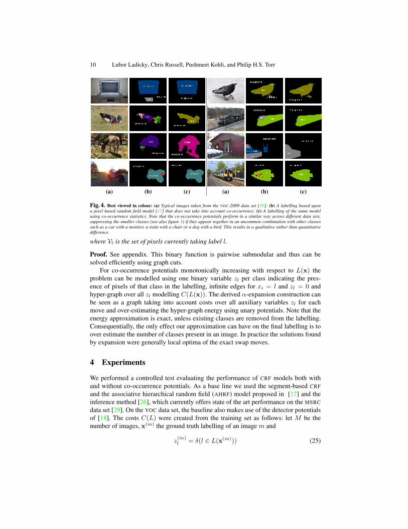
Fig. 4. Best viewed in colour: (a) Typical images taken from the VOC-2009 data set [29]; (b) A labelling based upona pixel based random field model [17] that does not take into account co-occurrence; (c) A labelling of the same modelusing co-occurrence statistics. Note that the co-occurrence potentials perform in a similar way across different data sets,suppressing the smaller classes (see also figure 1) if they appear together in an uncommon combination with other classessuch as a car with a monitor, a train with a chair or a dog with a bird. This results in a qualitative rather than quantitativedifference.

where Vl is the set of pixels currently taking label l.

Proof. See appendix. This binary function is pairwise submodular and thus can besolved efficiently using graph cuts.

For co-occurrence potentials monotonically increasing with respect to L(x) theproblem can be modelled using one binary variable zl per class indicating the pres-ence of pixels of that class in the labelling, infinite edges for xi = l and zl = 0 andhyper-graph over all zl modelling C(L(x)). The derived α-expansion construction canbe seen as a graph taking into account costs over all auxiliary variables zl for eachmove and over-estimating the hyper-graph energy using unary potentials. Note that theenergy approximation is exact, unless existing classes are removed from the labelling.Consequentially, the only effect our approximation can have on the final labelling is toover estimate the number of classes present in an image. In practice the solutions foundby expansion were generally local optima of the exact swap moves.

4 Experiments

We performed a controlled test evaluating the performance of CRF models both withand without co-occurrence potentials. As a base line we used the segment-based CRFand the associative hierarchical random field (AHRF) model proposed in [17] and theinference method [26], which currently offers state of the art performance on the MSRCdata set [29]. On the VOC data set, the baseline also makes use of the detector potentialsof [18]. The costs C(L) were created from the training set as follows: let M be thenumber of images, x(m) the ground truth labelling of an image m and

z(m)l = δ(l ∈ L(x(m))) (25)


an indicator function for label l appearing in an image m. The associated cost wastrained as:

C(L) = −w log1M

(1 +

M∑m=1

∏l∈L

z(m)l

), (26)

where w is the weight of the co-occurrence potential. The form guarantees, that C(L)is monotonically increasing with respect to L. To avoid over-fitting we approximatedthe potential C(L) as a second order function:

C ′(L) =∑l∈L

cl +∑

k,l∈L,k<l

ckl, (27)

where cl and clk minimise the mean-squared error between C(L) and C ′(L).On the MSRC data set we observed a 3% overall and 4% average per class increase

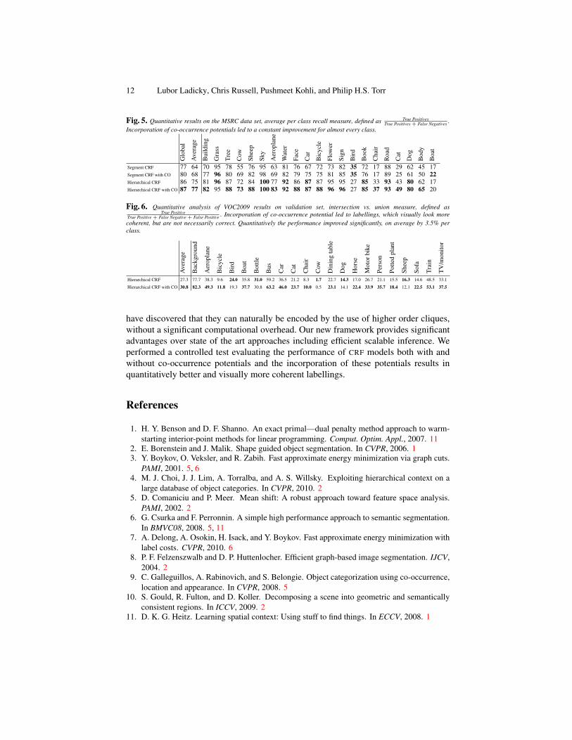
in the recall and 6% in the intersection vs. union measure with the of the segment-based CRF and a 1% overall, 2% average per class and 2% in the intersection vs. unionmeasure with the AHRF. The comparison on the VOC2009 data set was performed on thevalidation set, as the test set is not published and the number of permitted submissionsis limited. Performance improved by 3.5% in the intersection vs. union measure used inthe challenge. The performance on the test set was 32.11% which is comparable withcurrent state-of-the-art methods. Results for both data sets are given in tables 5 and 6.

By adding a co-occurrence cost into the CRF we observe constant improvement inpixel classification for almost all classes in all measures. In accordance with desiderata(iv), the co-occurrence potentials tend to suppress uncommon combination of classesand produce more coherent images in the labels space. This results in a qualitativerather than quantitative difference. Although the unary potentials already capture tex-tural context [29], the incorporation of co-occurrence potentials leads to a significantimprovement in accuracy.

It is not computationally feasible to perform a direct comparison between the work [22]and our potentials, as the AHRF model is defined over individual pixels, and it is notpossible to minimise the resulting fully connected graph which would contain approxi-mately 4×1010 edges. Similarly, without their scene classification potentials it was notpossible to do a like for like comparison with [31].

Average running time on the MSRC data set without co-occurrence was 5.1s in com-parison to 16.1s with co-occurrence cost. On the VOC2009 data set the average timeswere 107s and 388s for inference without respectively with co-occurrence costs. Wecompared the performance of α-expansion with LP relaxation using solver given in[1] for general co-occurrence potential on the sub-sampled images [16]. Both methodsproduced similar results in terms of energy, however α-expansion was approximately42, 000 times faster.

5 Conclusion

The importance of co-occurrence statistics has been well established [31,22,6]. In thiswork we have examined the use of co-occurrence statistics and how they might be incor-porated into a global energy or likelihood model such as a conditional random field. We


Fig. 5. Quantitative results on the MSRC data set, average per class recall measure, defined as True PositivesTrue Positives + False Negatives .

Incorporation of co-occurrence potentials led to a constant improvement for almost every class.

Glo

bal

Ave

rage

Bui

ldin

g

Gra

ss

Tree

Cow

Shee

p

Sky

Aer

opla

ne

Wat

er

Face

Car

Bic

ycle

Flow

er

Sign

Bir

d

Boo

k

Cha

ir

Roa

d

Cat

Dog

Bod

y

Boa

t

Segment CRF 77 64 70 95 78 55 76 95 63 81 76 67 72 73 82 35 72 17 88 29 62 45 17Segment CRF with CO 80 68 77 96 80 69 82 98 69 82 79 75 75 81 85 35 76 17 89 25 61 50 22Hierarchical CRF 86 75 81 96 87 72 84 100 77 92 86 87 87 95 95 27 85 33 93 43 80 62 17Hierarchical CRF with CO 87 77 82 95 88 73 88 100 83 92 88 87 88 96 96 27 85 37 93 49 80 65 20

Fig. 6. Quantitative analysis of VOC2009 results on validation set, intersection vs. union measure, defined asTrue Positive

True Positive + False Negative + False Positive . Incorporation of co-occurrence potential led to labellings, which visually look morecoherent, but are not necessarily correct. Quantitatively the performance improved significantly, on average by 3.5% perclass.

Ave

rage

Bac

kgro

und

Aer

opla

ne

Bic

ycle

Bir

d

Boa

t

Bot

tle

Bus

Car

Cat

Cha

ir

Cow

Din

ing

tabl

e

Dog

Hor

se

Mot

orbi

ke

Pers

on

Potte

dpl

ant

Shee

p

Sofa

Trai

n

TV

/mon

itor

Hierarchical CRF 27.3 77.7 38.3 9.6 24.0 35.8 31.0 59.2 36.5 21.2 8.3 1.7 22.7 14.3 17.0 26.7 21.1 15.5 16.3 14.6 48.5 33.1

Hierarchical CRF with CO 30.8 82.3 49.3 11.8 19.3 37.7 30.8 63.2 46.0 23.7 10.0 0.5 23.1 14.1 22.4 33.9 35.7 18.4 12.1 22.5 53.1 37.5

have discovered that they can naturally be encoded by the use of higher order cliques,without a significant computational overhead. Our new framework provides significantadvantages over state of the art approaches including efficient scalable inference. Weperformed a controlled test evaluating the performance of CRF models both with andwithout co-occurrence potentials and the incorporation of these potentials results inquantitatively better and visually more coherent labellings.

References

1. H. Y. Benson and D. F. Shanno. An exact primal—dual penalty method approach to warm-starting interior-point methods for linear programming. Comput. Optim. Appl., 2007. 11

2. E. Borenstein and J. Malik. Shape guided object segmentation. In CVPR, 2006. 13. Y. Boykov, O. Veksler, and R. Zabih. Fast approximate energy minimization via graph cuts.

PAMI, 2001. 5, 64. M. J. Choi, J. J. Lim, A. Torralba, and A. S. Willsky. Exploiting hierarchical context on a

large database of object categories. In CVPR, 2010. 25. D. Comaniciu and P. Meer. Mean shift: A robust approach toward feature space analysis.

PAMI, 2002. 26. G. Csurka and F. Perronnin. A simple high performance approach to semantic segmentation.

In BMVC08, 2008. 5, 117. A. Delong, A. Osokin, H. Isack, and Y. Boykov. Fast approximate energy minimization with

label costs. CVPR, 2010. 68. P. F. Felzenszwalb and D. P. Huttenlocher. Efficient graph-based image segmentation. IJCV,

2004. 29. C. Galleguillos, A. Rabinovich, and S. Belongie. Object categorization using co-occurrence,

location and appearance. In CVPR, 2008. 510. S. Gould, R. Fulton, and D. Koller. Decomposing a scene into geometric and semantically

consistent regions. In ICCV, 2009. 211. D. K. G. Heitz. Learning spatial context: Using stuff to find things. In ECCV, 2008. 1


12. D. Hoiem, C. Rother, and J. M. Winn. 3d layoutcrf for multi-view object class recognitionand segmentation. In CVPR, 2007. 6

13. P. Kohli, L. Ladicky, and P. Torr. Robust higher order potentials for enforcing label consis-tency. In CVPR, 2008. 14

14. V. Kolmogorov. Convergent tree-reweighted message passing for energy minimization.PAMI, 2006. 6

15. V. Kolmogorov and C. Rother. C.: Comparison of energy minimization algorithms for highlyconnected graphs. In ECCV, 2006. 6

16. L. Ladicky, C. Russell, P. Kohli, and P. Torr. Graph Cut based Inference with Co-occurrenceStatistics — Technical report, 2010. 6, 11

17. L. Ladicky, C. Russell, P. Kohli, and P. H. Torr. Associative hierarchical crfs for object classimage segmentation. In ICCV, 2009. 2, 3, 10

18. L. Ladicky, C. Russell, P. Sturgess, K. Alahari, and P. Torr. What, where and how many?Combining object detectors and CRFs. ECCV, 2010. 10

19. J. Lafferty, A. McCallum, and F. Pereira. Conditional random fields: Probabilistic modelsfor segmenting and labelling sequence data. In ICML, 2001. 2

20. D. Larlus and F. Jurie. Combining appearance models and markov random fields for categorylevel object segmentation. In CVPR, 2008. 2

21. M. Narasimhan and J. A. Bilmes. A submodular-supermodular procedure with applicationsto discriminative structure learning. In UAI, 2005. 9

22. A. Rabinovich, A. Vedaldi, C. Galleguillos, E. Wiewiora, and S. Belongie. Objects in context.In ICCV, 2007. 1, 2, 5, 6, 11

23. X. Ren, C. Fowlkes, and J. Malik. Mid-level cues improve boundary detection. TechnicalReport UCB/CSD-05-1382,Berkeley, Mar 2005. 1

24. C. Rother, S. Kumar, V. Kolmogorov, and A. Blake. Digital tapestry. In CVPR,2005. 925. B. Russell, W. Freeman, A. Efros, J. Sivic, and A. Zisserman. Using multiple segmentations

to discover objects and their extent in image collections. In CVPR, 2006. 226. C. Russell, L. Ladicky, P. Kohli, and P. Torr. Exact and approximate inference in associative

hierarchical networks using graph cuts. UAI, 2010. 6, 1027. B. Schlkopf and A. J. Smola. Learning with Kernels: Support Vector Machines, Regulariza-

tion, Optimization, and Beyond. Adaptive Computation and Machine Learning. MIT Press,2001. 3

28. J. Shi and J. Malik. Normalized cuts and image segmentation. PAMI,, 2000. 229. J. Shotton, J. Winn, C. Rother, and A. Criminisi. TextonBoost: Joint appearance, shape and

context modeling for multi-class object recognition and segmentation. In ECCV (1), 2006.1, 2, 3, 10, 11

30. R. Szeliski, R. Zabih, D. Scharstein, O. Veksler, V. Kolmogorov, A. Agarwala, M. Tappen,and C. Rother. A comparative study of energy minimization methods for markov randomfields. In ECCV, 2006. 4

31. A. Torralba, K. P. Murphy, W. T. Freeman, and M. A. Rubin. Context-based vision systemfor place and object recognition. In Computer Vision, Proceedings., 2003. 1, 2, 3, 4, 5, 11

32. T. Toyoda and O. Hasegawa. Random field model for integration of local information andglobal information. PAMI, 2008. 4, 5

33. Y. Weiss and W. Freeman. On the optimality of solutions of the max-product belief-propagation algorithm in arbitrary graphs. Transactions on Information Theory, 2001. 6

34. L. Yang, P. Meer, and D. J. Foran. Multiple class segmentation using a unified frameworkover mean-shift patches. In CVPR, 2007. 1


Appendix

Lemma 1 Proof. First we show that:

Eα(t) = minzα

[(Cαβ − Cβ)(1− zα) +

∑i∈Vαβ

(Cαβ − Cβ)(1− ti)zα]

={

0 if ∀i ∈ Vαβ : ti = 1,Cαβ − Cβ otherwise. (28)

If ∀i ∈ Vαβ : ti = 1 then∑i∈Vαβ (Cαβ − Cβ)(1 − ti)zα = 0 and the minimum cost

cost 0 occurs when zα = 1. If ∃i ∈ Vαβ , ti = 0 the minimum cost labelling occurswhen zα = 0 and the minimum cost is Cαβ − Cβ .

Similarly:

Eβ(t) = minzβ

[(Cαβ − Cα)zβ +

∑i∈Vαβ

(Cα,β − Cα)ti(1− zβ)]

={

0 if ∀i ∈ Vαβ : ti = 0,Cαβ − Cα otherwise. (29)

By inspection, if ∀i ∈ Vαβ : ti = 0 then∑i∈Vαβ (Cα,β − Cα)ti(1 − zβ) = 0 and

the minimum cost cost 0 occurs when zβ = 0. If ∃i ∈ Vαβ , ti = 1 the minimum costlabelling occurs when zβ = 1 and the minimum cost is Cαβ − Cα.

For all three cases (all pixels take label α, all pixels take label β and mixed labelling)E(t) = Eα(t) + Eβ(t) + Cα + Cβ − Cαβ . The construction of the αβ-swap move issimilar to the Robust PN model [13]. utSee figure 3 for graph construction.

Lemma 2 Proof. Similarly to the αβ-swap proof we can show:

Eα(t) = minzα

[k′α(1− zα) +

∑i∈V

k′α(1− ti)zα]

={k′α if ∃i ∈ V s.t. ti = 0,0 otherwise. (30)

If ∃i ∈ Vs.t.ti = 0, then∑i∈V k

′α(1− ti) ≥ k′α, the minimum is reached when zα = 0

and the cost is k′α.If ∀i ∈ V : ti = 1 then k′α(1 − ti)zα = 0, the minimum is reached when zα = 1 andthe cost becomes 0.

For all other l ∈ A:

Eb(t) = minzl

[k′′l zl +

∑i∈Vl

k′′l ti(1− zl)]

={k′′l if ∃i ∈ Vl s.t. ti = 1,0 otherwise. (31)

If ∃i ∈ Vl s.t. ti = 1, then∑i∈Vl k

′′l ti ≥ k′′l , the minimum is reached when zl = 1 and

the cost is k′′l .If ∀i ∈ Vl : ti = 0 then

∑i∈Vl k

′′l ti(1− zl) = 0, the minimum is reached when zl = 1

and the cost becomes 0.By summing up the cost Eα(t) and |A| costs El(t) we get E′(t) = Eα(t) +∑l∈AEl(t). If α is already present in the image k′α = 0 and edges with this weight

and variable zα can be ignored. utSee figure 3 for graph construction.

graph cut based inference with co-occurrence statisticslubor/eccv10co.pdf · graph cut based...

Documents