graph cuts and applicaton to disparity map estmaton
TRANSCRIPT

Renaud Marlet/Pascal Monasse 1
MVA/IMA – 3D Vision
Graph Cuts and Application toDisparity Map Estimation
Renaud Marlet
LIGM/École des Ponts ParisTech (IMAGINE) & Valeo.aiPascal Monasse
LIGM/École des Ponts ParisTech (IMAGINE)
(with many borrowings from Boykov & Veksler 2006)
Renaud Marlet/Pascal Monasse 2
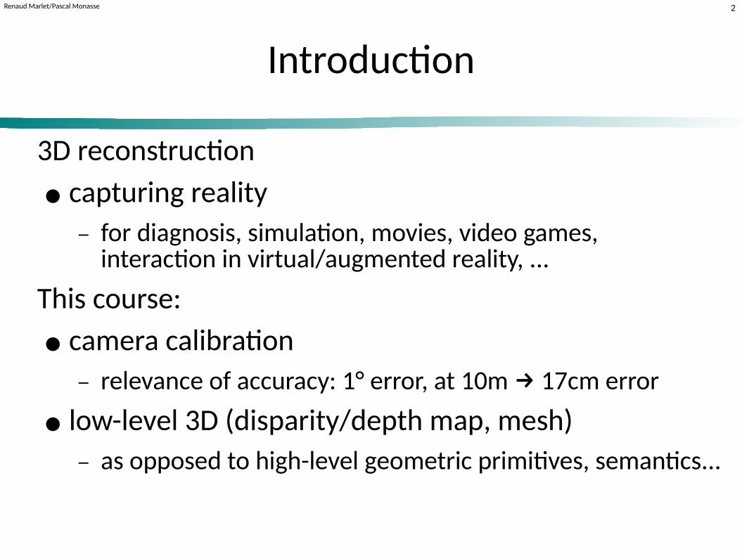
Introduction
3D reconstruction
● capturing reality
− for diagnosis, simulation, movies, video games, interaction in virtual/augmented reality, ...
This course:
● camera calibration
− relevance of accuracy: 1° error, at 10m 17cm errorcm error
● low-level 3D (disparity/depth map, mesh)
− as opposed to high-level geometric primitives, semantics...

Renaud Marlet/Pascal Monasse 3
Mathematical tools for 3D reconstruction
● Deep learning:
− very good for matching image regions
subcomponent of 3D reconstruction algorithm
− a few methods for direct disparity/depth map estimation− fair results on 3D reconstruction from single view
● Graph cuts (this lecture):
− practical, well-founded, general ( maps, meshes...)
Gro
uei
x et
al.
20
17cm error

Renaud Marlet/Pascal Monasse 4
● Powerful multidimensional energy minimization tool− wide class of binary and non binary energies− in some cases, globally optimal solutions− some provably good approximations (and good in practice)− allowing regularizers with contrast preservation
■ enforcement of piecewise smoothnesswhile preserving relevantsharp discontinuities
● Geometric interpretation− hypersurface in n-D space
Motivating graph cuts
Yan
g, W
ang
& A
hu
ja 2
010
© IE
EEB
oyk
ov
& V
eksl
er 2
006
© S
pri
nge
r
E( f ) = ∑
p∈P Dp( f
p)
+ ∑(p,q)∈N V
p,q( f
p, f
q)

Renaud Marlet/Pascal Monasse 5
Many links to other domains
− Combinatorial algorithms (e.g., dynamic programming)
− Simulated annealing
− Markov random fields (MRFs)
− Random walks and electric circuit theory
− Bayesian networks and belief propagation
− Level sets and other variational methods
− Anisotropic diffusion
− Statistical physics
− Submodular functions
− Integral/differential geometry, etc.
(cf. Boykov & Veksler 2006)
dynamic programming = programmation dynamiquesimulated annealing = recuit simuléMarkov random field = champ (aléatoire) de Markovrandom walk = marche aléatoireBayesian network = réseaux bayésienlevel set = ligne de niveausubmodular function = fonction sous-modulaire

Renaud Marlet/Pascal Monasse 6
Overview of the course
● Notions
− graph cut, minimum cut
− flow network, maximum flow
− optimization: exact (global), approximate (local)
● Illustration with emblematic applications
segmentation disparity map estimation

Renaud Marlet/Pascal Monasse 7cm error
Overview of the course
● Notions
− graph cut, minimum cut
− flow network, maximum flow
− optimization: exact (global), approximate (local)
● Illustration with emblematic applications
segmentation disparity map estimation
No time to go deep
into every topic →
general ideas,
read the references

Renaud Marlet/Pascal Monasse 8
Graph cuts basics
Max-flow min-cut theorem
Application to image restorationand image segmentation
Part 1

Renaud Marlet/Pascal Monasse 9
Graph cut basics
● Graph G ⟨V,E ⟩ (digraph)− set of nodes (vertices) V− set of directed edges E
■ p q
● V {s, t }∪P
− terminal nodes: {s, t }
■ s: source node■ t: target node (= sink)
− non-terminal nodes: P■ ex. P = set of pixels, voxels, etc.
(can be very different from an image)
Bo
yko
v &
Vek
sler
200
6 ©
Sp
rin
ger
node = nœudvertex (vertices) = sommet(s)edge = arêtedirected = orientédigraph (directed graph) = graphe orientésink = puits
Example of connectivity

Renaud Marlet/Pascal Monasse 10
Graph cut basics
● Edge labels, for pq ∈E− c(p,q) ≥ 0: nonnegative costs
also called weights w(p,q)
− c(p,q) and c(q,p), if any, may differ
● Links
− t-link: term. ↔ non-term.
■ {s p | p≠ t }, {q t | q≠ s }
− n-link: non-term. non-term.
■ N {p q | p,q ≠ s,t}
Boykov & Veksler 2006 © Springer
c(p,q)
label = étiquetteweight = poidslink = lien

Renaud Marlet/Pascal Monasse 11
Cut and minimum cut
● s-t cut (or just “cut”): C = {S,T }
node partition such that s ∈ S, t ∈ T
● Cost of a cut {S,T }:
− c(S,T ) = ∑p∈S, q∈T c(p,q)
− N.B. cost of severed edges:only from S to T
● Minimum cut:
− i.e., with min cost: minS,T c(S,T )
− intuition: cuts only “weak” links
Boykov & Veksler 2006 © SpringerBoykov & Veksler 2006 © Springer
cut
cut = coupesevered = coupé, sectionné
c(p,q)

Renaud Marlet/Pascal Monasse 12
Different view: flow network
● Different vocabulary and features■ graph ↔ network
vertex = node p, q, …edge = arc p
q or (p,q)
cost = capacity c(p,q)
− possibly many sources & sinks
● Flow f : V × V ℝ− f(p,q): amount of flow p
q
■ (p,q) ∉ E ⇔ c(p,q) = 0, f(p,q) = 0
− e.g. road traffic, fluid in pipes, current in electrical circuit, ...
Boykov & Veksler 2006 © Springer
f(p,q)/c(p,q)
flow = flotnetwork = réseautransportation = transportvertex = sommetnode = nœudedge = arête
(or transportation network)

Renaud Marlet/Pascal Monasse 13
Flow network constraints
● Capacity constraint− f(p,q) ≤ c(p,q)
● Skew symmetry− f(p,q) = −f(q,p)
● Flow conservation
− ∀p, net flow ∑q∈V f(p,q) = 0
unless p = s (s produces flow) or p = t (t consumes flow)
− i.e., incoming ∑(q,p)∈E f(q,p)
= outgoing ∑(p,q)∈E f(p,q)
Boykov & Veksler 2006 © Springer
f(p,q)/c(p,q)
skew symmetry = antisymétrie
p
q3
q4
q2
2
3
4q
1
1
Kirchhoff's law

Renaud Marlet/Pascal Monasse 14
Flow network constraints
● s-t flow (or just “flow) f − f : V × V ℝ
satisfying flow constraints
● Value of s-t flow− | f | = ∑
q∈V f(s,q) = ∑p∈V f(p,t)
■ amount of flow from source= amount of flow to sink
● Maximum flow:
− i.e., with maximum value: maxf | f |
− intuition: arcs saturated as much as possible
Boykov & Veksler 2006 © Springer
f(p,q)/c(p,q)
skew symmetry = antisymétrie

Renaud Marlet/Pascal Monasse 15
Max-flow min-cut theorem
● TheoremThe maximum value of an s-t flow is equal to theminimum capacity (i.e., min cost) of an s-t cut.
● Example− | f | = c(S,T ) = ?
s
3/3
t
1/2
1/1
3/41/1
1/4
0/2 0/32/2
S
T
edge label: c(p,q)

Renaud Marlet/Pascal Monasse 16
Max-flow min-cut theorem
● TheoremThe maximum value of an s-t flow is equal to theminimum capacity (i.e., min cost) of an s-t cut.
● Example− | f | = c(S,T ) = 4− min: enumerate partitions...
s
3/3
t
1/2
1/1
3/41/1
1/4
0/2 0/32/2
S
T
edge label: c(p,q)
Renaud Marlet/Pascal Monasse 17cm error
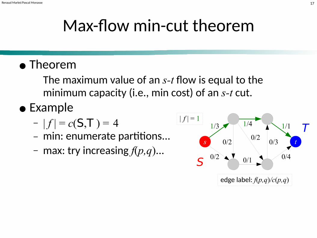
Max-flow min-cut theorem
● TheoremThe maximum value of an s-t flow is equal to theminimum capacity (i.e., min cost) of an s-t cut.
● Example− | f | = c(S,T ) = 4− min: enumerate partitions... − max: try increasing f(p,q)...
s
1/3
t
0/2
1/1
0/40/1
1/4
0/2 0/30/2
S
T
edge label: f(p,q)/c(p,q)
| f | = 1

Renaud Marlet/Pascal Monasse 18
Max-flow min-cut theorem
● TheoremThe maximum value of an s-t flow is equal to theminimum capacity (i.e., min cost) of an s-t cut.
● Example− | f | = c(S,T ) = 4− min: enumerate partitions... − max: try increasing f(p,q)...
s
2/3
t
0/2
1/1
1/40/1
1/4
0/2 0/31/2
S
T
edge label: f(p,q)/c(p,q)
| f | = 2

Renaud Marlet/Pascal Monasse 19
Max-flow min-cut theorem
● TheoremThe maximum value of an s-t flow is equal to theminimum capacity (i.e., min cost) of an s-t cut.
● Example− | f | = c(S,T ) = 4− min: enumerate partitions... − max: try increasing f(p,q)...
s
3/3
t
0/2
1/1
2/40/1
1/4
0/2 0/32/2
S
T
edge label: f(p,q)/c(p,q)
| f | = 3

Renaud Marlet/Pascal Monasse 20
Max-flow min-cut theorem
● TheoremThe maximum value of an s-t flow is equal to theminimum capacity (i.e., min cost) of an s-t cut.
● Example− | f | = c(S,T ) = 4− min: enumerate partitions... − max: try increasing f(p,q)...
s
3/3
t
1/2
1/1
3/41/1
1/4
0/2 0/32/2
S
T
edge label: f(p,q)/c(p,q)
| f | = 4

Renaud Marlet/Pascal Monasse 21
Max-flow min-cut theorem
● TheoremThe maximum value of an s-t flow is equal to theminimum capacity (i.e., min cost) of an s-t cut.
● Example− | f | = c(S,T ) = 4− min: enumerate partitions... − max: try increasing f(p,q)...
● Intuition− pull s and t apart: the graph tears where it is weak− min cut: cut corresponding to a small number of weak links− max flow: flow bounded by low-capacity links in a cut
s
3/3
t
1/2
1/1
3/41/1
1/4
0/2 0/32/2
S
T
to pull = tirerto tear = (se) déchirerweak = faible
edge label: f(p,q)/c(p,q)

Renaud Marlet/Pascal Monasse 22
Max-flow min-cut theorem
● TheoremThe maximum value of an s-t flow is equal to the minimum capacity (i.e., min cost) of an s-t cut.
− proved independentlyby Elias, Feinstein & Shannon,and Ford & Fulkerson (1956)
− special case of strong duality theoremin linear programming
− can be used to derive other theorems
linear programmaing = programmationlinéaire

Renaud Marlet/Pascal Monasse 23
Max flows and min cuts configurationsare not unique
● Different configurations with same maximum flow
● Different configurations with same min-cut cost
1/2
0/4
1/1
0/3
1/10/2
1/4
0/1
1/3
1/10.3/2
0.7/4
0.3/1
0.7/3
1/1
1/11/1 1/11/1
edge label: f(p,q)/c(p,q)

Renaud Marlet/Pascal Monasse 24
Algorithms for computing max flow
● Polynomial time
● Push-relabel methods
− better performance for general graphs
− e.g. Goldberg and Tarjan 1988: O(V E
log(V2/E))
■ where V: number of vertices, E: number of edges
● Augmenting paths methods
− iteratively push flow from source to sink along some path
− better performance on specific graphs
− e.g. Ford-Fulkerson 1956: O(E max|f |) for integer capacity c
Renaud Marlet/Pascal Monasse 25
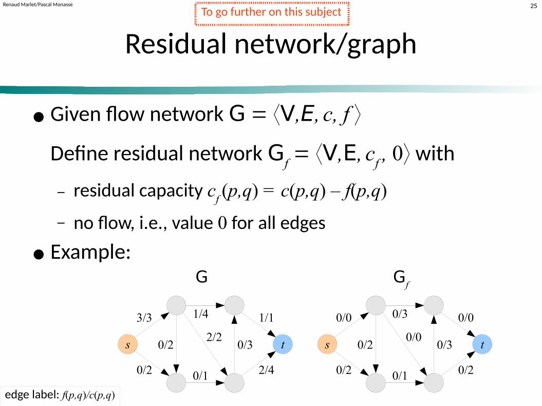
Residual network/graph
● Given flow network G ⟨V,E, c, f ⟩
Define residual network Gf ⟨V,E,
c
f , 0⟩ with
− residual capacity cf (p,q) = c(p,q) – f(p,q)
− no flow, i.e., value 0 for all edges
● Example:
s
3/3
t
0/2
1/1
2/40/1
1/4
0/2 0/32/2
s
0/0
t
0/2
0/0
0/20/1
0/3
0/2 0/30/0
G Gf
edge label: f(p,q)/c(p,q)
To go further on this subject

Renaud Marlet/Pascal Monasse 26
Ford-Fulkerson algorithm (1956)
● N.B. termination not guaranteed
− maximum flow reached if (semi-)algorithm terminates(but may “converge” to less than maximum flow if it does not terminate)
− always terminates for integer values (or rational values)
f(p,q) 0 for all edges [P: augmenting path]while ∃ path P
from s to t
such that ∀(p,q)
∈
P
c
f (p,q) > 0
cf (P) min{c
f (p,q) | (p,q) ∈ P} [min residual capacity]
for each edge (p,q) ∈ P f(p,q) f(p,q) + c
f (P) [push flow along path]
f(q,p) f(q,p) – cf (P) [keep skew symmetry]
termination = terminaisonsemi-algorithm: termination not guaranteed for all inputs
To go further on this subject

Renaud Marlet/Pascal Monasse 27cm error
Ford-Fulkerson algorithm: an example
s
0/3
t
0/2
0/1
0/40/1
0/4
0/2 0/30/2
3:0
t
2:0 1:0
4:0
2:03:0
2:0s t
2:0
1:0
4:01:0
4:0
2:03:0
2:0
s
1/3
t
0/2
1/1
0/40/1
1/4
0/20/3
0/2s
2:1
t
2:0
0:1
4:01:0
3:1
2:03:0
2:0 s t
2:0
0:1
4:01:0
3:1
2:03:0
2:0
s
3/3
t
0/2
1/1
2/40/1
1/4
0/20/3
2/2s
0:3
t
2:0
0:1
2:21:0
3:1
2:03:0
0:2 s
0:3
t
2:0
0:1
2:2
min=13:1
2:03:0
0:2
f / c
s
3/3
t
1/2
1/1
3/41/1
1/4
0/20/3
2/2s
0:3
t
1:1
0:1
1:30:1
3:1
2:03:0
0:2
4:0
| f | = 1+2+1 = 4 = c(S,T)
s
3
t
2
1
41
4
2 32
cf (P):c
f
s
3:0
min=22:1
min=11:0
1:0
cf : c
f (= c-c
f )
No more P s.t. cf(P) > 0
To go further on this subject

Renaud Marlet/Pascal Monasse 28
Ford-Fulkerson algorithm: an example
s
0/3
t
0/2
0/1
0/40/1
0/4
0/2 0/30/2
3:0
t
2:0 1:0
4:0
2:03:0
2:0s t
2:0
1:0
4:01:0
4:0
2:03:0
2:0
s
1/3
t
0/2
1/1
0/40/1
1/4
0/20/3
0/2s
2:1
t
2:0
0:1
4:01:0
3:1
2:03:0
2:0 s t
2:0
0:1
4:01:0
3:1
2:03:0
2:0
s
2/3
t
0/2
1/1
1/41/1
1/4
1/20/3
0/2s
1:2
t
2:0
0:1
3:10:1
3:1
1:13:0
2:0 s
1:2
t
2:0
0:1
3:1
3:1
1:13:0
2:0
s
2/3
t
1/2
1/1
2/41/1
1/4
0/20/3
1/2s
1:2
t
1:1
0:1
2:20:1
3:1
2:03:0
1:1
4:0
s
3:0
2:1
1:0
0:1
s
1:2
t
1:1
0:1
2:2
min=13:1
2:03:0
1:1
0:1
| f | = 1+1+1+1 = 4 = c(S,T)
Taking edges backwards = OK (and sometimes needed)
min=1
min=1
min=1
f / c cf (P):c
fcf : c
f (= c-c
f )
To go further on this subject

Renaud Marlet/Pascal Monasse 29
Edmonds-Karp algorithm (197cm error2)
● As Ford-Fulkerson but shortest path with >0 capacity− breadth-first search for augmenting path (cf. example above)
● Termination: now guaranteed
● Complexity: O(V E2)
− slower than push-relabel methods for general graphs
− faster in practice for sparse graphs
● Other variant (Dinic 197cm error0), complexity: O(V2 E)
− other flow selection (blocking flows)
− O(V E
log
V) with dynamic trees (Sleator & Tarjan 1981)
breadth-first = en largeur d'abordsparse = épars, peu dense
To go further on this subject

Renaud Marlet/Pascal Monasse 30
Maximum flow for grid graphs
● Fast augmenting path algorithm(Boykov & Kolmogorov 2004)
− often significantly outperforms push-relabel methods
− observed running time is linear
− many variants since then
● But push-relabel algorithm can be run in parallel
− good setting for GPU acceleration
The “best” algorithm depends on the context

Renaud Marlet/Pascal Monasse 31
Variant: Multiway cut problem
● More than two terminals: {s1,...,s
k}
● Multiway cut:
− set of edges leaving each terminal in a separate component
● Multiway cut problem
− find cut with minimum weight
− same as min cut when k = 2 − NP-hard if k ≥ 3 (in fact APX-hard, i.e., NP-hard to approx.)
− but can be solved exactly for planar graphs
planar = planaire
To go further on this subject

Renaud Marlet/Pascal Monasse 32
Graph cuts for binary optimization
● Inherently a binary technique
− splitting in two
● 1st use in image processing:binary image restoration (Greig et al. 1989)
− black&white image with noise image with no noise
● Can be generalized to large classes of binary energy
− regular functions

Renaud Marlet/Pascal Monasse 33
Binary image restoration
noise
© Mark Schmidt 2007cm error
threshold
graph cut
noise = bruitthreshold = seuil

Renaud Marlet/Pascal Monasse 34
Binary image restoration:The graph cut view
● Agreement with observed data
− Dp(l): penalty (= -reward) for assigning
label l ∈ {0,1} to pixel p∈P
− if Ip=l then D
p(l) < D
p(l') for l'≠l
− w(s,p)=Dp(1), w(p,t)=D
p(0)
● Example:− if I
p = 0, D
p(0) = 0, D
p(1) = κ
if Ip
= 1, Dp(0) = κ, D
p(1) = 0
− if Ip
= 0 and p∈S, cost = Dp(0) = 0
if Ip
= 0 and p∈T, cost = Dp(1) = κ
penalty = pénalité, coûtreward = récompense
Dp
(1) =
κ
ST
sink ↔ 1 (white)
source ↔ 0 (black)
p qλ
Dp
(0)
λ
Dq
(1) = 0
Dq
(0) =
κ
Bo
yko
v &
Vek
sler
200
6 ©
Sp
rin
ger
Ip : intensity of image I at pixel p

Renaud Marlet/Pascal Monasse 35
Binary image restoration:The graph cut view
● Agreement with observed data
− Dp(l): penalty (= ‒reward) for assigning
label l ∈ {0,1} to pixel p∈P
− if Ip=l then D
p(l) < D
p(l') for l'≠l
− w(s,p)=Dp(1), w(p,t)=D
p(0)
● Minimize discontinuities
− penalty for (long) contours
■ w(p,q) = w(q,p) = λ > 0
− spatial coherence, regularizing constraint,smoothing factor... (see below)
penalty = pénalité, coûtreward = récompenseregularizing constraint = contrainte de régularisationsmoothing = lissage
ST
sink ↔ 1 (white)
source ↔ 0 (black)
p qλ
Dp
(0)
λ
Dq
(1) = 0
Dp
(1) =
κ
Dq
(0) =
κ
Bo
yko
v &
Vek
sler
200
6 ©
Sp
rin
ger

Renaud Marlet/Pascal Monasse 36
Binary image restoration:The graph cut view
labeling = étiquetage
ST
sink ↔ 1 (white)
source ↔ 0 (black)
p qλ
Dp
(0)
λ
Dq
(1) = 0
Dp
(1) =
κ
Dq
(0) =
κ
Bo
yko
v &
Vek
sler
200
6 ©
Sp
rin
ger
● Binary labeling f [N.B. different from “flow f ”]
− assigns label fp ∈
{0,1} to pixel p∈P
■ f : P → {0,1} f(p) = fp
● Cut C = {S,T } ↔ labeling f − 1-to-1 correspondence: f = 1|T
● Cost of a cut: | C
| =
∑p∈P Dp
(fp) + ∑
(p,q)∈S×T w(p,q)
= cost of flip + cost of local dissimilarity
● Restored image:= labeling corresponding to a minimum cut

Renaud Marlet/Pascal Monasse 37cm error
Binary image restoration:The energy view
● Energy of labeling f
− E( f ) ≝ |
C
| =
∑p∈P Dp
(fp) +
λ ∑(p,q)∈N 1(f
p = 0∧ f
q = 1)
where
1(false) = 0 | 1(true) = 1
[or: ½ λ ∑(p,q)∈N 1(f
p ≠ f
q)]
● Restored image:− labeling corresponding to
minimum energy (= minimum cut)
ST
sink ↔ 1 (white)
source ↔ 0 (black)
p qλ
Dp
(0)
λ
Dq
(1) = 0
Dp
(1) =
κ
Dq
(0) =
κ
Bo
yko
v &
Vek
sler
200
6 ©
Sp
rin
ger

Renaud Marlet/Pascal Monasse 38
Binary image restoration:The smoothing factor
● Small λ (actually λ/κ):
− pixels choose their label independentlyof their neighbors
● Large λ:
− pixels choose the labelwith smaller average cost
● Balanced λ value:
− pixels form compact, spatiallycoherent clusters with same label
− noise/outliers conform to neighbors
cluster = amasoutlier = point aberrant
ST
sink ↔ 1 (white)
source ↔ 0 (black)
p qλ
Dp
(0) = 0
λ
Dq
(1) = 0
Dp
(1) =
κ
Dq
(0) =
κ
Bo
yko
v &
Vek
sler
200
6 ©
Sp
rin
ger

Renaud Marlet/Pascal Monasse 39
Graph cuts for energy minimization
● Given some energy E( f ) such that
− f : P → L = {0,1} binary labeling
− E( f ) = ∑p∈P Dp
(fp) + ∑
(p,q)∈N Vp,q
(fp , fq
)
− regularity condition (see below) V
p,q(0,0) + V
p,q(1,1) ≤ V
p,q(0,1) + V
p,q(1,0)
● Theorem: then there is a graph whose minimum cut defines a labeling f that reaches the minimum energy (Kolmogorov & Zabih 2004) [N.B. Vladimir Kolmogorov, not Andrey Kolmogorov]
[structure of graph somehow similar to above form]
Edata
( f ) Eregul
( f )

Renaud Marlet/Pascal Monasse 40
Graph construction
● Preventing a t-link cut: “infinite” weight
● Favoring a t-link cut: null weight (≈ no edge)
● Bidirectional edge vs monodirectional & back edges
0
s t
∞
s t
∞
s t
0
∞
s t
∞
0
0
w w
w
ww
⇔ ⇔∞
S TS TS T

Renaud Marlet/Pascal Monasse 41
Graph cuts as hypersurfaces
● Cut on a 2D grid
N.B. Several “seeds” (sources and sinks)
● Cut on a 3D grid
Boykov & Veksler 2006 © Springer
(cf. Boykov & Veksler 2006)
seed = graine
To go further on this subject

Renaud Marlet/Pascal Monasse 42
Example of topological issue
● Connected seeds ● Disconnected seeds
Boykov & Veksler 2006 © Springer
seed = graine
To go further on this subject

Renaud Marlet/Pascal Monasse 43
Example of topological constraint:fold prevention
● Ex. in disparity map estimation: d = f(x,y)
● In 2D: y = f(x), only one value for y given one x
Boykov & Veksler 2006 © Springer
x
y
disparity map = carte de disparité
To go further on this subject

Renaud Marlet/Pascal Monasse 44
A “revolution” in optimization
● Previously (before Greig et al. 1989)
− exact optimization like this was not possible
− used approaches:■ iterative algorithms such as simulated annealing
■ very far from global optimum, even in binary case like this
■ work of Greig et al. was (primarily) meant to show this fact
● Remained unnoticed for almost 10 years in the computer vision community...
■ maybe binary image restoration was viewed as too restrictive ?(Boykov & Veksler 2006)
simulated annealing = recuit simulé

Renaud Marlet/Pascal Monasse 45
Graph cut techniques: now very popular in computer vision
● Extensive work since 1998− Boykov, Geiger, Ishikawa, Kolmogorov, Veksler, Zabih
and others...
● Almost linear in practice (in nb nodes/edges)− but beware of the graph size :
it can be exponential in the size of the problem
● Many applications− regularization, smoothing, restoration
− segmentation
− stereovision: disparity map estimation, ...

Renaud Marlet/Pascal Monasse 46
Warning:global optimum ≠ best real-life solution
● Graph cuts provide exact, global optimum
− to binary labeling problems (under regularity condition)
● But the problem remains a model
− approximation of reality
− limited number of factors
− parameters (e.g., λ)
☛ Global optimum of abstracted problem,
not necessarily best solution in real life

Renaud Marlet/Pascal Monasse 47cm error
Not for free
● Many papers construct
− their own graph
− for their own specific energy function
● The construction can be fairly complex
☛ Powerful tool but does not exempt from thinking(contrary to some aspects of deep learning )

Renaud Marlet/Pascal Monasse 48
Graph cut vs deep learning
● Graph cut
− works well, with proven optimality bounds
● Deep learning
− works extremely well, but mainly empirical
● Somewhat complementary
− graph cut sometimes used to regularize network output

Renaud Marlet/Pascal Monasse 49
Application to image segmentation
● Problem:
− given an image with foreground objects and background
− given sample areas of both kinds (O, B)
− separate objects from background
background = arrière-plansample = échantillonarea = zone
[Duchenne & al. 2008]

Renaud Marlet/Pascal Monasse 50
Application to image segmentation
● Problem:
− given an image with foreground objects and background
− given sample areas of both kinds (O, B)
− separate objects from background
background = arrière-plansample = échantillonarea = zone
OB

Renaud Marlet/Pascal Monasse 51
Intuition
What characterizes an object/background segmentation ?
OB

Renaud Marlet/Pascal Monasse 52
Intuition
What characterizes an object/background segmentation ?
− pixels of segmented object and backgroundlook like corresponding sample pixels O and B
− segment contours have high gradient, and are not too long
OB
background = arrière-plansample = échantillonarea = zone
Renaud Marlet/Pascal Monasse 53
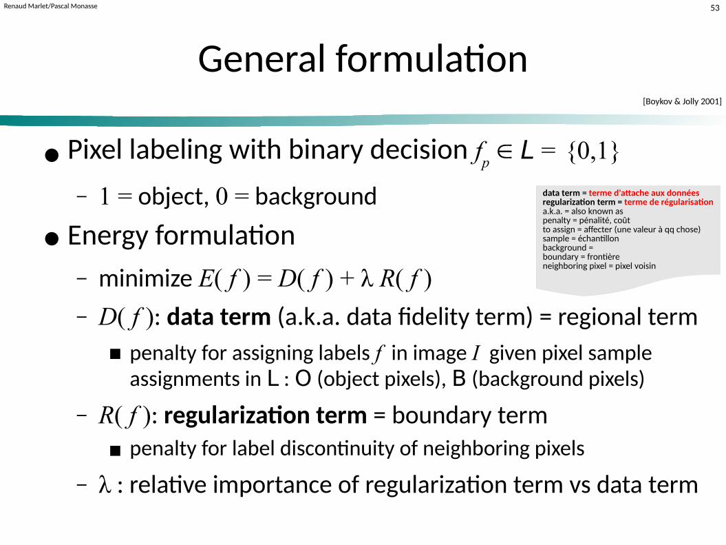
General formulation
● Pixel labeling with binary decision fp ∈ L = {0,1}
− 1 = object, 0 = background
● Energy formulation
− minimize E( f ) = D( f ) + λ R( f )− D( f ): data term (a.k.a. data fidelity term) = regional term
■ penalty for assigning labels f in image I given pixel sample assignments in L : O (object pixels), B (background pixels)
− R( f ): regularization term = boundary term■ penalty for label discontinuity of neighboring pixels
− λ : relative importance of regularization term vs data term
[Boykov & Jolly 2001]
data term = terme d'attache aux donnéesregularization term = terme de régularisationa.k.a. = also known aspenalty = pénalité, coûtto assign = affecter (une valeur à qq chose)sample = échantillonbackground = boundary = frontièreneighboring pixel = pixel voisin

Renaud Marlet/Pascal Monasse 54
Probabilisticjustification/framework
● Minimize E( f ) ↔ maximize posterior proba. Pr( f | I ) ● Bayes theorem:
Pr( f | I ) Pr(I ) = Pr(I | f ) Pr( f )
● Consider likelihoods L( f | I ) = Pr(I | f
)
● Actually consider log-likelihoods (→ sums)E( f ) = D( f )
+
λ
R( f ) −log Pr( f |
I
)
+
c = −log Pr(I
| f ) −log Pr( f )
↔ data term,probability to
observe image Iknowing labeling f
A constant(independent of f )
↔ regularization term,depending on type of labelingand with various hypotheses(e.g., locality, cf. MRF below)
The term wantto maximize
w.r.t. f
posterior probability = probabilité a posteriorilikelihood = vraisemblance(log-)likelihood = (log-)vraisemblance
To go further on this subject

Renaud Marlet/Pascal Monasse 55
Data term:linking estimated labels to observed pixels
● D( f ) and likelihood
− penalty for assigning labels f in I given sample assignments ↔ (log-)likelihood that
f is consistent with image samples
− D( f ) = − log L( f | I ) = − log Pr(I | f
)
● Pixel independence hypothesis (common approximation)
− Pr(I | f ) = ∏p∈P Pr(I
p| f
p) if pixels iid ( )
− D( f ) = ∑p∈P Dp
( fp)
where D
p( f
p ) = −log Pr(I
p | f
p)
■ Dp( f
p ) : penalty for observing I
p for a pixel of type f
p
☛ Find an estimate of Pr(Ip | f
p)
penalty = pénalité, coûtto assign = affectersample = échantillonlikelihood = vraisemblancerandom variable = variable aléatoire
independent and identicallydistributed random variables
wrong strictlyspeaking, but “true enough”
to be oftenassumed
To go further on this subject

Renaud Marlet/Pascal Monasse 56
Data term:likelihood/color model
● Approaches to find an estimate of Pr(Ip| f
p)
− histograms■ build an empirical distribution of the
color of object/background pixels, based on pixels marked as object/background
■ estimate Pr(Ip | fp
) based on histograms: Premp
(rgb|O),Premp
(rgb|B)
− Gaussian Mixture Model (GMM)■ model the color of object (resp. background) pixels
with a distribution defined as a mixture of Gaussians
− texon (or texton): texture patch (possibly abstracted)■ compare with expected texture property:
response to filters (spectral analysis), moments...
Blunsden 2006 @ U. of Edinburgh
© C
ano
n 2
012
empirical probability = probabilité empirique (fréquence relative)Gaussian mixture = mélange de gaussiennes
To go further on this subject

Renaud Marlet/Pascal Monasse 57cm error
Markov random field = champ de Markovrandom variable = variable aléatoireneighborhood = voisinageundirected graph = graph non orientégraphical model = modèle graphique
Regularization term: locality hypotheses
● Markov random field (MRF), or Markov network
− neighborhood system: N = {Np | p ∈ P }
■ Np : set neighbors of p such that p ∉ N
p and p ∈ N
q ⇔ q ∈ N
p
− X = (Xp)
p∈P : field (set) of random variables
such that each random variable Xp depends
on other random variables only through its neighbors N
p
locality hypothesis: Pr(Xp = x |
XP∖{p}
) = Pr(Xp = x |
XNp
)
− N ≈ undirected graph: (p,q) edge iff p ∈ Nq (
⇔ q ∈ N
p )
(MRF also called undirected graphical model)
To go further on this subject

Renaud Marlet/Pascal Monasse 58
Regularization term: locality hypotheses
● Gibbs random field (GRF)− G undirected graph, X = (X
p)
p∈P random variables such that
Pr(X = x) ∝ exp(− ∑C clique of G V
C (x))
■ clique = complete subgraph: ∀p≠q∈C (p,q)∈G
■ VC
: clique potential = prior probability of the given realization of the
elements of the clique C (fully connected subgraph)
● Hammersley-Clifford theorem (197cm error1)− If probability distribution has positive mass/density, i.e.,
if Pr(X = x) > 0 for all x, then: X MRF w.r.t. graph N iff X GRF w.r.t. graph N
provides a characterization of MRFs as GRFs
Gibbs random field = champ de Gibbsundirected graph = graph non orientéclique = clique (!)clique potential = potentiel de cliqueprior probability = probabilité a posteriori
© B
attiti
& B
run
ato
200
9
To go further on this subject

Renaud Marlet/Pascal Monasse 59
Regularization term: locality hypotheses
● Hypothesis 1: only 2nd-order cliques (i.e., edges)
R( f ) = − log Pr( f ) = − log exp(−∑(p,q) edge of G V
(p,q) ( f )) [GRF]
= ∑(p,q)∈N Vp,q
( fp ,fq
) [MRF pairwise potentials]
● Hypothesis 2: (generalized) Potts model
Vp,q
( fp ,f
q) = B
p,q 1( fp ≠
fq)
i.e., Vp,q
( fp ,f
q) = 0 if f
p =
fq
Vp,q
( fp ,f
q) = B
p,q if f
p ≠
fq
(Origin: statistical mechanics− spin interaction in crystalline lattice− link with “energy” terminology)
[Boykov, Veksler & Zabih 1998]
pairwise = par pairepairwise potential = potentiel d'ordre 2Potts model = modèle de Pottsstatistical mechanics = physique statistique
To go further on this subject

Renaud Marlet/Pascal Monasse 60
Examples of boundary penalties (ad hoc)
● Penalize label discontinuity at intensity continuity
− Bp,q
= exp(−(Ip−I
q)2/2σ2) / dist(p,q)
■ large between pixels of similar intensities, i.e., when | Ip−I
q | < σ
■ small between pixels of dissimilar intensities, i.e., when | Ip−I
q | > σ
■ decrease with pixel distance dist(p,q) [here: 1 or √2]■ ≈ distribution of noise among neighboring pixels
● Penalize label discontinuity at low gradient
− Bp,q
= g(|| ∇Ip ||) with g positive decreasing
■ e.g., g(x) = 1/(1 + c x2)■ penalization for label discontinuity at low gradient
[Boykov & Jolly 2001]
To go further on this subject
Renaud Marlet/Pascal Monasse 61
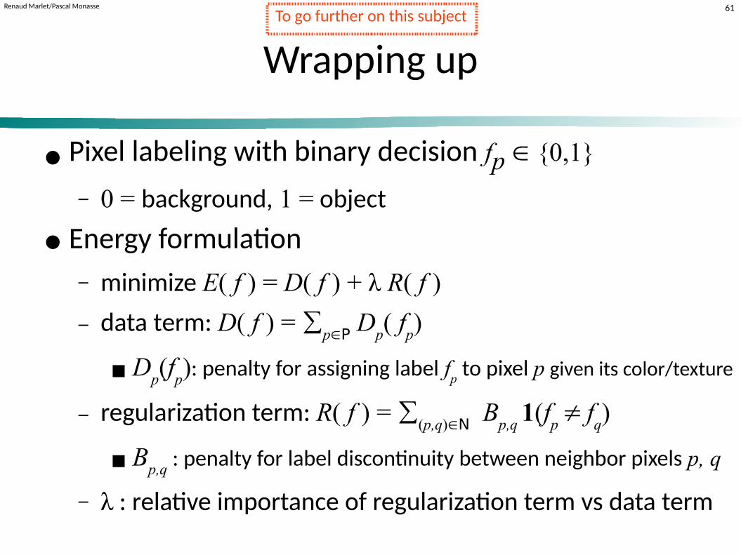
Wrapping up
● Pixel labeling with binary decision fp ∈ {0,1}
− 0 = background, 1 = object
● Energy formulation
− minimize E( f ) = D( f ) + λ R( f )
− data term: D( f ) = ∑p∈P Dp
( fp)
■ Dp(f
p): penalty for assigning label f
p to pixel p given its color/texture
− regularization term: R( f ) = ∑(p,q)∈N B
p,q 1(f
p ≠
fq)
■ Bp,q
: penalty for label discontinuity between neighbor pixels p, q
− λ : relative importance of regularization term vs data term
To go further on this subject

Renaud Marlet/Pascal Monasse 62
Graph-cut formulation (version 1)
● Direct expression as graph-cut problem: − V = {s,t}∪P− E = {(s,p) | p∈P } ∪ {(p,q) | p,q∈N } ∪ {(p,t) | p∈P }
− E( f ) = ∑p∈P Dp
(fp) + λ ∑
(p,q)∈N Bp,q
1(fp ≠
fq)
■ ex. Dp(l) = −log Pr
emp(I
p| f
p =
l) [empirical probability for O et B]
■ ex. Bp,q
= exp(−(Ip−I
q)2/2σ2) / dist(p,q)
Edge Weight Sites
(p,q) λ Bp,q (p,q) ∈ N
(s,p) Dp(1) p ∈ P
(p,t) Dp(0) p ∈ P
Warning:the connexity N
is specific tothe problem !
source ↔ 0(background)
sink ↔ 1(foreground object)

Renaud Marlet/Pascal Monasse 63
Graph-cut formulation (version 1)
● Direct expression as graph-cut problem: − V = {s,t}∪P− E = {(s,p) | p∈P } ∪ {(p,q) | p,q∈N } ∪ {(p,t) | p∈P }
− E( f ) = ∑p∈P Dp
(fp) + λ ∑
(p,q)∈N Bp,q
1(fp ≠
fq)
● Any problem/risk with this formulation ?
Edge Weight Sites
(p,q) λ Bp,q (p,q) ∈ N
(s,p) Dp(1) p ∈ P
(p,t) Dp(0) p ∈ P
source ↔ 0(background)
sink ↔ 1(foreground object)

Renaud Marlet/Pascal Monasse 64
Graph-cut formulation (version 1)
● Direct expression as graph-cut problem: − V = {s,t}∪P− E = {(s,p) | p∈P } ∪ {(p,q) | p,q∈N } ∪ {(p,t) | p∈P }
− E( f ) = ∑p∈P Dp
(fp) + λ ∑
(p,q)∈N Bp,q
1(fp ≠
fq)
● Pb: pixels of object/background samples not necessarily assigned with good label !
Edge Weight Sites
(p,q) λ Bp,q (p,q) ∈ N
(s,p) Dp(1) p ∈ P
(p,t) Dp(0) p ∈ P
source ↔ 0(background)
sink ↔ 1(foreground object)

Renaud Marlet/Pascal Monasse 65
Graph-cut formulation (version 2)
● Obj/Bg samples now always labeled OK in minimal f *
− where K = 1 + maxp∈P λ ∑
(p,q)∈N B
p,q
K ≈ +∞, i.e., too expensive to pay ⇒ label never assigned
Edge Weight Sites
(p,q) λ Bp,q (p,q) ∈ N
(s,p)
Dp(1) p ∈ P, p ∉ (O ∪ B)
K p ∈ B
0 p ∈ O
(p,t)
Dp(0) p ∈ P, p ∉ (O ∪ B)
0 p ∈ B
K p ∈ O
[Boykov & Jolly 2001]
source ↔ 0(background)
sink ↔ 1(foreground object)

Renaud Marlet/Pascal Monasse 66
Some limitations(here with simple color model)
● Is the segmentation OK ?
To go further on this subject

Renaud Marlet/Pascal Monasse 67cm error
Some limitations(here with simple color model)
color modelnot complex
enough
neighboringmodel
not complexenough
sensitivity toregularization
parameter
To go further on this subject

Renaud Marlet/Pascal Monasse 68
Exercise 1: implement simpleimage segmentation using graph cuts
● Load image and display it● Get object/background samples with mouse clicks (e.g.,
small square area around mouse position) and draw them● Define graph as in course (version 2)
− choose neighbor connectivity [ 4: or 8: ]− choose one of B
p,q expressions defined in course
− model color of object/background with 1 single gaussian centered around mean color
■ write Pr(Ip| f
p) w.r.t. mean color of obj/bg: what is D
p(f
p) then ?
● Compute max flow, extract cut, display image segments● Experiment with various parameters (λ, σ, c, ...)● And comment what you observe
To go further on this subject

Renaud Marlet/Pascal Monasse 69
Multi-label problems
Exact vs approximate solutions
Application to stereovision(disparity/depth map estimation):
disparity/depth ↔ label
Part 2

Renaud Marlet/Pascal Monasse 7cm error0
Two-label (binary) problem
− P : set of sites (pixels, voxels...)
− N : set of neighboring site pairs
− L = {0,1} : binary labels
− f : P → L binary labeling [notation: fp = f(p) = l ]
− E : (P → L) → ℝ : energy
■ E( f ) = ∑p∈P Dp
(fp) + ∑
(p,q)∈N Vp,q
(fp , fq
)
− Dp(l): label penalty for site p
− Vp,q
(l,l'): prior knowledge about optimal pairwise labeling
● Pb: find f * that reaches the minimum energy E( f *)
Edata
( f ) Eregul
( f )
Renaud Marlet/Pascal Monasse 7cm error1
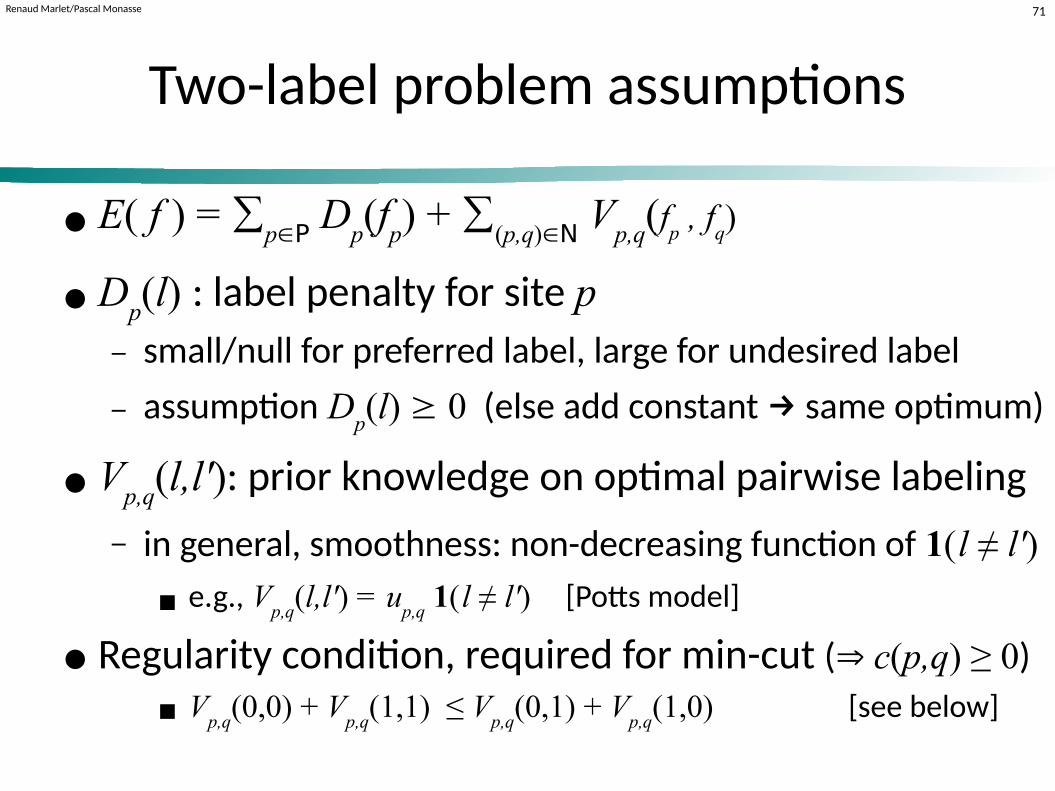
Two-label problem assumptions
● E( f ) = ∑p∈P Dp
(fp) + ∑
(p,q)∈N Vp,q
(fp , fq
)
● Dp(l) : label penalty for site p
− small/null for preferred label, large for undesired label
− assumption Dp(l) ≥ 0 (else add constant → same optimum)
● Vp,q
(l,l'): prior knowledge on optimal pairwise labeling
− in general, smoothness: non-decreasing function of 1( l ≠ l')
■ e.g., Vp,q
(l,l') = up,q 1(
l ≠ l') [Potts model]
● Regularity condition, required for min-cut (⇒ c(p,q) ≥ 0)
■ Vp,q
(0,0) + Vp,q
(1,1) ≤ Vp,q
(0,1) + Vp,q
(1,0) [see below]

Renaud Marlet/Pascal Monasse 7cm error2
Multi-label problem
− P : set of sites (pixels, voxels...)
− N : set of neighboring site pairs
− L : finite set of labels (→ can model scalar or even vector)
■ e.g., discretization of intensity, stereo disparity, motion vector...
− f : P → L labeling
− E : (P → L) → ℝ : energy
■ E( f ) = ∑p∈P Dp
(fp) + ∑
(p,q)∈N Vp,q
(fp , fq
) = Edata
( f ) + Eregul
( f )
− Dp(l): label penalty for site p
− Vp,q
(lp,l
q): prior knowledge about optimal pairwise labeling
● Pb: find f * that reaches the minimum energy E( f *)
disparity = disparité

Renaud Marlet/Pascal Monasse 7cm error3
Multi-label problem assumptions
● E( f ) = ∑p∈P Dp
(fp) + ∑
(p,q)∈N Vp,q
(fp , fq
)
● Dp(l) : label penalty for site p
− small for preferred label, large for undesired label
− assumption Dp(l) ≥ 0 (else add constant → same optimum)
● Vp,q
(lp,l
q): prior knowledge on optimal pairwise labeling
− in general, smoothness prior:non-decreasing function of || l
p ‒ l
q || [norm used if vector]
■ e.g., Vp,q
(lp,l
q) = λ
p,q || l
p ‒ l
q ||
■ smaller penalty for closer labels
smoothness = lissage

Renaud Marlet/Pascal Monasse 7cm error4
Graph cuts for“general” energy minimization
● Problem: find labeling f * : P L minimizing energyE(
f ) = ∑
p∈P Dp( f
p) + ∑
(p,q)∈N Vp,q
( fp, f
q)
● Question: can a globally optimal labeling f * be found using some graph-cut construction?
● Answer:
− binary labeling: yes iff Vp,q
is regular (Kolmogorov & Zabih 2004)
Vp,q
(0,0) + Vp,q
(1,1) ≤ Vp,q
(0,1) + Vp,q
(1,0) [otherwise NP-hard]
− multi-labeling: yes if Vp,q
convex (Ishikawa 2003)
and if L linearly ordered (⇒ 1D only ⇒ not 2D motion vector)
− otherwise: approximate solutions (but some very good)

Renaud Marlet/Pascal Monasse 7cm error5
Piecewise-smooth vs everywhere-smooth
● Observation: object propertiesoften smooth everywhere except on boundaries
☛ Consequence: piecewise-smooth models moreappropriate than everywhere-smooth models
Yan
g, W
ang
& A
hu
ja 2
010
© IE
EE
piecewise = par morceaux
piecewise smoothinguniform smoothingoriginal

Renaud Marlet/Pascal Monasse 7cm error6
Piecewise-smooth modelsvs everywhere-smooth models
● Local variation of potentials Vp,q
depending on label variation
l'
l
l'
l
locally smooth from l to l'when going from p to p'
lp
lq
Vp,q
(lp,l
q)
piecewise-smooth potential
p
Vp,q
lp' p p'
locally steep from l to l'when going from p to p'
steep = raide, très pentu

Renaud Marlet/Pascal Monasse 7cm error7cm error
Piecewise-smooth potentialsvs everywhere-smooth potentials
● General graph construction forany convex V
p,q (Ishikawa 2003)
− convex ⇒ large penalty for sharp jump
− a few small jumps cheaper than one large jump
− ☛ discontinuities smoothed with “ramp” ⇒ oversmoothing
lp
lq
Vp,q
(lp,l
q)
In practice,best results with“least convex”function, e.g.,
Vp,q
(lp,l
q) = λ
p,q || l
p ‒ l
q ||
lp
lq
Vp,q
(lp,l
q)

Renaud Marlet/Pascal Monasse 7cm error8
Discontinuity-preserving energy
● At edges, very different labels for adjacent pixels are OK
● To not overpenalize in Eadjacent but very different labels:
− Vp,q
non-convex function of || lp ‒ l
q ||
− for instance (cap max):
■ Vp,q
= min(K, || lp −
lq ||2)
■ Vp,q
= min(K, || lp − lq ||)
■ Vp,q
= up,q
1( lp ≠ l
q) (Potts model)
lp
lq
Vp,q
(lp,l
q)
Renaud Marlet/Pascal Monasse 7cm error9
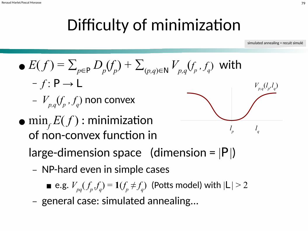
Difficulty of minimization
● E( f ) = ∑p∈P Dp
(fp) + ∑
(p,q)∈N V
p,q(f
p , fq) with
− f : P → L
− Vp,q
(fp , fq
) non convex
● minf E( f ) : minimization
of non-convex function in
large-dimension space (dimension = |P |) − NP-hard even in simple cases
■ e.g. Vpq
( fp ,f
q) = 1( fp
≠ fq) (Potts model) with |L | > 2
− general case: simulated annealing...
simulated annealing = recuit simulé
lp
lq
Vp,q
(lp,l
q)

Renaud Marlet/Pascal Monasse 80
Exact binary optimization (reminder)
● Pb: find labeling f * : P L = {0,1} minimizing energyE(
f ) = ∑
p∈P Dp( f
p) + ∑
(p,q)∈N Vp,q
( fp, f
q)
● Question:− can a globally optimal labeling f * be found using
some graph-cut construction?
● Answer (Kolmogorov & Zabih 2004):− yes iff V
pq is regular
■ Vp,q
(0,0) + Vp,q
(1,1) ≤ Vp,q
(0,1) + Vp,q
(1,0)
− otherwise it's NP-hard
● But what about general energies on binary variables ?

Renaud Marlet/Pascal Monasse 81
Exact binary optimization
● Question: − what functions can be minimized using graph cuts?
● Classes of functions on binary variables:− F 2: E(
x
1,...,x
n) = ∑
i Ei(x
i)
+
∑
i<j Ei,j(x
i, x
j)
− F 3: E( x
1,...,x
n) = ∑
i Ei(x
i)
+
∑
i<j Ei,j(x
i, x
j)
+
∑
i<j<k Ei,j,k(x
i, x
j, x
k)
− F m: E( x
1,...,x
n) = ∑
i Ei(x
i) + … + ∑
u1<...<um Eu1,...,um(x
u1, ...
, x
um)
● “Using graph cuts”: E graph-representable iff∃ graph G ⟨V,E ⟩ with V = {v
1,...,v
n, s, t}
such that
∀configuration x=x1,...,x
n , E(
x
1,...,x
n) = cost(min s-t-cut in
which vi ∈S if x
i =
0 and v
i ∈T if x
i =
1) + k constant ∈
ℝ
[Kolmogorov & Zabih 2004]
m-th order potentials

Renaud Marlet/Pascal Monasse 82
Exact binary optimization
● E regular iff
− F 2: ∀i,j Ei,j(0,0) + Ei,j(1,1) ≤ Ei,j(0,1) + Ei,j(1,0)
− F m: for all terms Eu1,...,um in E, all projections (specializations) of Eu1,...,um to a two-variable function (i.e., all variables fixed but two) are regular
● Question:
− what functions can be minimized using graph cuts?
● Answer (Kolmogorov & Zabih 2004):
− F 2, F 3: E graph-representable ⇔ E regular− any binary E: E not regular ⇒ E not graph-representable
[Kolmogorov & Zabih 2004]
To go further on this subject

Renaud Marlet/Pascal Monasse 83
Link with submodularity
● g : 2P ℝ submodular
− iff g(X ) + g(Y
) ≥ g(X ∪
Y
) + g(X ∩
Y
)
for any X, Y ⊂ P
− iff g(X ∪ {j}) − g(X
) ≥ g(X ∪
{i,j}) − g(X ∪
{j})
for any X ⊂ P and i, j ∈
P
∖ X
● g submodular ⇔ E regular, with E(x) = g({ p ∈ P | xp=1})
− Ei,j(0,1) + Ei,j(1,0) ≥ Ei,j(0,0) + Ei,j(1,1)
● independent results on submodular functions
− minimization in polynomial time but slow, best known O(n6)
submodular = sous-modulaire
To go further on this subject

Renaud Marlet/Pascal Monasse 84
Exact multi-label optimization(for 2nd-order potentials)
● Problem: find labeling f * : P L minimizing energyE(
f ) = ∑
p∈P Dp( f
p) + ∑
(p,q)∈N Vp,q
( fp, f
q)
● Assumption: L linearly ordered — w.l.o.g. L = {1,...,k}(1D only ⇒ not suited, e.g., for 2D motion vector estimation)
● Solution: reduction/encoding to binary label case
■ for Vp,q
(lp ,l
q) = λ
p,q | lp ‒ l
q | (Boykov et al. 1998, Ishikawa & Geiger 1998)
■ for any convex Vp,q
(Ishikawa 2003)
− See also− MinSum pbs (Schlesinger & Flach 2006)
− submodular Vp,q
(Darbon 2009)
linearly ordered = linéairement ordonnéw.l.o.g. = without loss of generality

Renaud Marlet/Pascal Monasse 85
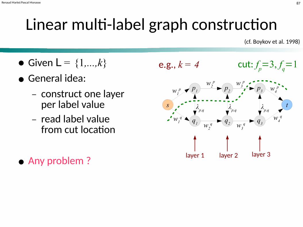
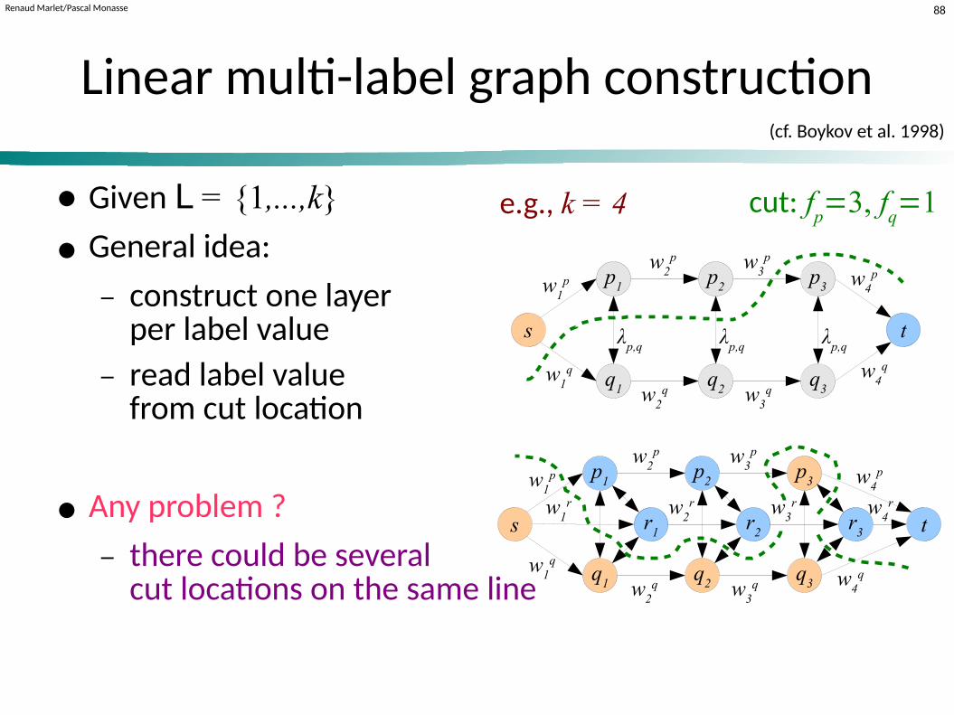
Linear multi-label graph construction
● Given L = {1,...,k}
● General idea:
− construct one layerper label value
− read label value from cut location
(cf. Boykov et al. 1998)
s
p1t
1p
q1
q3
p3
t
p2
q2
t2
p t3
p
t4
p
t2
q
t2
p
t3
q
t4
q
t2
p
t1
q
layer = couche
layer 1 layer 2 layer 3
cut: fp=3, f
q=1e.g., k = 4
s
t
layer 1
12
34
56

Renaud Marlet/Pascal Monasse 86
Linear multi-label graph construction
● E( f ) = ∑
p∈P Dp( f
p) + ∑
(p,q)∈N λ
p,q | fp ‒ f
q |
with fp ∈
L = {1,...,k}
Attempt 1:● For each site p
− create nodes p1 ,...,p
k‒1
− create edges t1
p = (s,p1), t
jp = (p
j-1,p
j), t
kp = (p
k-1,t)
− assign weights wjp = w(t
jp) = D
p(j)
● For each pair of neighboring sites p and q
− create edges (pj ,q
j)
j∈{1,...,k‒1} with weight λ
p,q
● Read label value from cut location, e.g., p2 ∈ S, p
3 ∈ T ⇒ f
p =
3
s
p1w
1p
q1
q3
p3
t
p2
q2
w2
p w3
p
w4
p
w2
q w3
qw
4qw
1q
λp,q
λp,q
λp,q
(cf. Boykov et al. 1998)
cut: fp=3, f
q=1
Renaud Marlet/Pascal Monasse 87cm error
Linear multi-label graph construction
● Given L = {1,...,k}
● General idea:
− construct one layerper label value
− read label value from cut location
● Any problem ?
(cf. Boykov et al. 1998)
layer 1 layer 2 layer 3
cut: fp=3, f
q=1e.g., k = 4
s
p1w
1p
q1
q3
p3
t
p2
q2
w2
p w3
p
w4
p
w2
q w3
qw
4qw
1q
λp,q
λp,q
λp,q
Renaud Marlet/Pascal Monasse 88
Linear multi-label graph construction
● Given L = {1,...,k}
● General idea:
− construct one layerper label value
− read label value from cut location
● Any problem ?
− there could be severalcut locations on the same line
s
p1w
1p
q1
q3
p3
t
p2
q2
w2
p w3
p
w4
p
w2
q w3
q w4
qw1
q
r1
r2
r3
w1
r w2
r w3
r w4
r
(cf. Boykov et al. 1998)
cut: fp=3, f
q=1e.g., k = 4
s
p1w
1p
q1
q3
p3
t
p2
q2
w2
p w3
p
w4
p
w2
q w3
qw
4qw
1q
λp,q
λp,q
λp,q

Renaud Marlet/Pascal Monasse 89
Linear multi-label graph construction
● E( f ) = ∑
p∈P Dp( f
p) + ∑
(p,q)∈N λ
p,q | fp ‒ f
q |
with fp ∈
L = {1,...,k}
Attempt 2:● For each site p
− create nodes p1 ,...,p
k‒1
− create edges t1
p = (s,p1), t
jp = (p
j-1,p
j), t
kp = (p
k-1,t)
− assign weights wjp = w(t
jp) = D
p(j) + K
p [penalize more cutting t
jp]
with Kp
= 1 +
(k‒1) ∑
q∈Np λ
p,q (where N
p set of neighbors of p)
● For each pair of neighboring sites p and q
− create edges (pj ,q
j)
j∈{1,...,k‒1} with weight λ
p,q
(cf. Boykov et al. 1998)
cut: fp=3, f
q=1
s
p1w
1p
q1
q3
p3
t
p2
q2
w2
p w3
p
w4
p
w2
q w3
qw
4qw
1q
λp,q
λp,q
λp,q

Renaud Marlet/Pascal Monasse 90
Linear multi-label graph properties
● Lemma: for each site p, a minimum cut severs exactly one tjp
− [≥1] Any cut severs at least one tjp
− [≤1] Suppose ta
p, tb
p are cut (same line p), then build new cut
with tbp restored and links (p
j ,q
j)
j∈{1,...,k‒1} broken for q
∈
N
p
Impact on (minimum) cost: − w(tb
p) + (k‒1) ∑q∈Np
λp,q
= − Dp(j)− 1 < 0 strictly smaller cost contradiction
● Theorem (Boykov et al. 1998): a minimum cut minimizes E( f )
s
p1t
1p
q1
q3
p3
t
p2
q2
t2
p t3
p
t4
p
t2q t
3q
t4
qt1
q
λp,q
λp,q
λp,q
(cf. Boykov et al. 1998)
s
p1t
1p
q1
q3
p3
t
p2
q2
t2
p t3
p
t4
p
t2
q
t2
p
t3
qt4
q
t2
p
t1
q
λp,q
λp,q
λp,q
severed = coupé, sectionné

Renaud Marlet/Pascal Monasse 91
Application to stereovision:disparity map estimation
● Problem
− given 2 rectified images I , I'
,
estimate optimal disparityd(p) = d
p for each pixel p = (u,v)
● Graph-cut setting
− discrete disparities: dp ∈ L = {d
min,...,d
max}
− data term: Dp(d
p)
■ small when pixel p in I similar to pixel p' = p +(dp ,0) in I'
− smoothness term: Vp,q
(dp , d
q)
■ small when disparities dp and d
q are similar
I I'
rectified images ↔ aligned cameras
p p' = p +(dp ,0)

Renaud Marlet/Pascal Monasse 92
Application to stereovision:disparity map estimation
● Problem
− given 2 rectified images I , I'
,
estimate optimal disparityd(p) = d
p for each pixel p = (u,v)
● Graph-cut setting
− discrete disparities: dp ∈ L = {d
min,...,d
max}
− data term: Dp(d
p)
■ small when pixel p in I similar to pixel p' = p +(dp ,0) in I'
− smoothness term: Vp,q
(dp , d
q)
■ small when disparities dp and d
q are similar
p p' = p +(dp ,0)
e.g., whatdefinition?
e.g., whatdefinition?
I I'

Renaud Marlet/Pascal Monasse 93
Application to stereovision:disparity map estimation
● Problem
− given 2 rectified images I , I'
,
estimate optimal disparityd(p) = d
p for each pixel p = (u,v)
● Graph-cut setting
− discrete disparities: dp ∈ L = {d
min,...,d
max}
− data term: Dp(d
p)
■ e.g., Dp(d
p) = E
ZNSSD(P
p ; (d
p ,0)) where P
p patch around pixel p
− smoothness term: Vp,q
(dp , d
q)
■ e.g., Vp,q
(dp , d
q) = λ |
d
p −
d
q | [Boykov et al. optimal disparities]
e.g., whatdefinition?
e.g., whatdefinition?
p p' = p +(dp ,0)
P P'
EZNSSD
(P ;
u) = 1/|P| ∑q∈P [(I'q+u
− I'P)
/ σ'
−
(Iq
− IP)
/ σ]2
σ = [1/|P| ∑q∈P (Iq −
IP)2 ]1/2IP = 1/|P| ∑q∈P Iq
I I'
SSD = sum of square differencesNSSD = normalized …ZNSSD = zero-normalized ...

Renaud Marlet/Pascal Monasse 94
Application to stereovision:disparity map estimation
● Problem
− given 2 rectified images I , I'
,
estimate optimal disparityd(p) = d
p for each pixel p = (u,v)
● Graph-cut setting
− discrete disparities: dp ∈ L = {d
min,...,d
max}
− data term: Dp(d
p)
■ e.g., Dp(d
p) = E
ZNSSD(P
p ; (d
p ,0))
− smoothness term: Vp,q
(dp , d
q)
■ e.g., Vp,q
(dp , d
q) = λ |
d
p −
d
q | [Boykov et al. optimal disparities]
Is it the “optimal” solutionto the disparity map
estimation problem ?
p p' = p +(dp ,0)
P P'
I I'

Renaud Marlet/Pascal Monasse 95
Application to stereovision:disparity map estimation
● Problem
− given 2 rectified images I , I'
,
estimate optimal disparityd(p) = d
p for each pixel p = (u,v)
● Graph-cut setting
− discrete disparities: dp ∈ L = {d
min,...,d
max}
− data term: Dp(d
p)
■ e.g., Dp(d
p) = E
ZNSSD(P
p ; (d
p ,0))
− smoothness term: Vp,q
(dp , d
q)
■ e.g., Vp,q
(dp , d
q) = λ |
d
p −
d
q | [Boykov et al. optimal disparities]
- Meaningful but arbitrary choices: patch size, similarity, smoothness... - Optimal solution for energy ⇒ optimal solution for problem
p p' = p +(dp ,0)
P
/
P'
I I'

Renaud Marlet/Pascal Monasse 96
Application to stereovision:disparity map estimation
● Problem
− given 2 rectified images I , I'
,
estimate optimal disparityd(p) = d
p for each pixel p = (u,v)
● Graph-cut setting (alternative)
− discrete disparities: dp ∈ L = {d
min,...,d
max}
− Dp(d
p)
=
w
cc ρ(E
ZNCC(P
; (d
p ,0)) with ρ(c) ∈ [0,1] ↘
■ e.g.
− Vp,q
(dp , d
q) = λ |
d
p −
d
q |
ρ(c) = { 1 if c < 0√1−c if c ≥ 0
0 1-1
1
ρ(c)
p p' = p +(dp ,0)
P
dissimilar similar equal
P'
N.B. only wcc
/ λ matters
I I'
EZNCC
(P ;
u) = 1/|P| ∑q∈P [(I'q+u
− I'P)
/ σ'
. (Iq
− IP)
/ σ]
σ = [1/|P| ∑q∈P (Iq −
IP)2 ]1/2I
P = 1/|P| ∑q∈P Iq
EZNSSD
(P ;
u) = 2
−
2
E
ZNCC(P
;
u)
0
CC = cross-correlationNCC = normalized …ZNCC = zero-normalized ...

Renaud Marlet/Pascal Monasse 97cm error
Approximate optimization
● Exact multi-label optimization:
− only limited cases
− in practice, may require large number of nodes
● How to go beyond exact optimization constraints?
☛ Iterate exact optimizations on subproblems (Boykov et al. 2001)
− local minimum ☹
− but within known bounds of global minimum ☺
bound = borne

Renaud Marlet/Pascal Monasse 98
Notion of move — Examples
Boykov et al. 2001 © IEEE
α β at one site
only
α ↔ β at many sites
at once
any l α at many sites
at once
Move: maps a labeling f : P L to a labeling f ' : P LIdea: iteratively apply moves to get closer to optimum f *
at once = à la foismove = déplacement (≈ modification) de la solution

Renaud Marlet/Pascal Monasse 99
Moves
Given a labeling f : P L and labels α, β
● f ' is a standard move from f ifff and f ' differ at most on one site p
● f ' is an expansion move (or α-expansion) from f iff∀p ∈ P, f '
p = f
p or α
in f ', compared to f, extra sites p can now be labeled α
● f ' is a swap move (or α-β-swap) from f iff∀p ∈ P, f
p ≠ α,β f
p = f '
p
some sites that were labeled α are now β and vice versa
N.B. Other kinds of moves can be defined...
move = déplacement (≈ modification) de la solutionα-β-swap = permutation α-β

Renaud Marlet/Pascal Monasse 100
Optimization w.r.t. moves
● Iterative optimization over moves− random cycle over all labels until convergence local min
● Iterating standard moves= usual discrete optimization method− iterated conditional modes (ICM) = iterative maximization
of the probability of each variable conditioned on the rest■ local minimum w.r.t. standard move,
i.e., energy cannot decrease with a single pixel label difference⇒ weak condition, low quality
− simulated annealing, ...■ slow convergence (optimal properties “at infinity”),
modest quality, some sampling strategies but mostly random
(cf. Boykov et. al 2001)
simulated annealing = recuit simulésampling = échantionnage

Renaud Marlet/Pascal Monasse 101
Optimization w.r.t. moves
● Iterative optimization over moves− random cycle over all labels until convergence local min
● Iterating expansion/swap moves (strong moves)− number of possible moves exponential in number of sites
− compute optimal move using graph cut = binary problem!■ see Boykov et. al 2001 for graph construction and details
− significantly fewer local minima than with standard moves
− sometimes within constant factor of global minimum■ e.g., expansion moves & Potts model optimum within factor 2
(cf. Boykov et. al 2001)

Renaud Marlet/Pascal Monasse 102
Image restoration with moves
● Restoration with standard moves vs α-expansions
Boykov et al. 2001 © IEEE
restoration withα-expansions
restoration withstandard moves
original image noisy image

Renaud Marlet/Pascal Monasse 103
● Expansion move: V metric, expansion inequality:
Vp,q
(α,α) + Vp,q
(β,γ) ≤ Vp,q
(α,γ) + Vp,q
(β,α) for all α,β,γ ∈
L
● Swap move: V semi-metric, swap inequality:
Vp,q
(α,α) + Vp,q
(β,β) ≤ Vp,q
(α,β) + Vp,q
(β,α) for all α,β ∈
L
[= as metric but triangle inequality not required: Vp,q
(α,γ) ≤ Vp,q
(α,β) + Vp,q
(β,γ)][weaker condition than for expansion move]
● Examples
− Potts model: Vp,q
(α,β) = λp,q
1(α ≠ β)
− truncated L2 distance: V
p,q(α,β)
=
min(K,||
α
−
β
||)
metric = métrique (= fonct distance)d(x,y) = 0 x = yd(x,y) = d(y,x) ≥ 0d(x,z) ≤ d(x,y)+d(y,z)
Constraints on interaction potential(see details in Boykov et. al 2001)
/discontinuity-preserving!
semi-metric = semimétriqued(x,y) = 0 x = yd(x,y) = d(y,x) ≥ 0
Renaud Marlet/Pascal Monasse 104
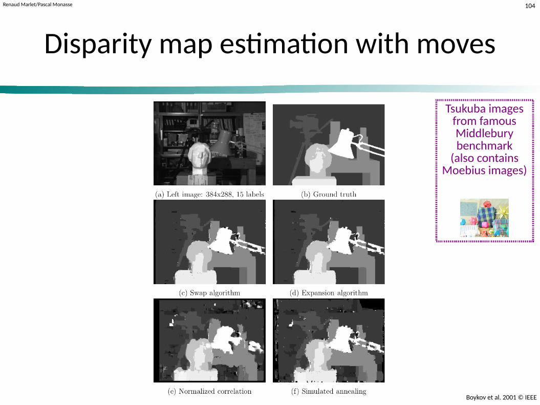
Disparity map estimation with moves
Boykov et al. 2001 © IEEE
Tsukuba imagesfrom famousMiddleburybenchmark
(also containsMoebius images)

Renaud Marlet/Pascal Monasse 105
Disparity map estimation:alternative data term
● Idea: direct intensity comparison, but sensitive to sampling
− Dp(d
p) = min(K , |I
p−I'
p+dp|2)
● With image sampling insensitivity:
− disparity range discretized to 1 pixel accuracy sensitivity to high gradients
− (sub)pixel dissimilarity measure for greater accuracy,e.g., by linear interpolation (Birchfield & Tomasi 1998)
− Cfwd
(p,d) = mind−1/2 ≤ u ≤ d+1/2
|Ip−I'
p+u|
− Crev
(p,d) = minp−1/2 ≤ x ≤ p+1/2
|Ix−I'
p+d| [for symmetry]
− Dp(d
p) = C(p,d
p) = min(K, C
fwd(p,d
p), C
rev(p,d
p))2
(cf. Boykov et al. 1999,Boykov et al. 2001)
No patch similarity here:the local consistency is givenby the smoothness term
To go further on this subject

Renaud Marlet/Pascal Monasse 106
Disparity map estimation:smoothness term
● Scene with fronto-parallel objects
− piecewise-constant model = OK
− e.g., Potts model:
Vp,q
(dp,d
q) = u
p,q 1(d
p ≠ d
q)
● Scene with slanted surfaces (e.g., ground)
− piecewise-smooth model = better
− e.g., smooth cap max value:
Vp,q
= λ min(K, |dp−d
q|)
● Metric ⇒ both swap and expansion algorithms usable

Renaud Marlet/Pascal Monasse 107cm error
Potts model vs smooth cap max value
Bo
yko
v et
al.
200
1 ©
IEEE
● Potts model : piecewise-constant
− suited for uniform areas (⇒ fewer disparities on large areas)
● Smooth cap max value: piecewise-smooth model
− suited for slowly-varying areas (e.g., slope)

Renaud Marlet/Pascal Monasse 108
Disparity map estimation:smoothness term
● Contextual information
− neighbors p,q more likely to have same disparity if Ip ≈ I
q
make Vp,q
(dp,d
q) also depend on |
I
p −
I
q |
− meaningful in low texture areas (where | I
p −
I
q | meaningful)
● E.g., with Potts model: Vp,q
(dp,d
q) = u
p,q 1(d
p ≠ d
q)
− up,q
: penalty for assigning different disparities to p and q− textured regions: u
p,q = K
− textureless regions: up,q
= U( | I
p −
I
q | )
■ up,q
smaller for pixels p,q with large intensity difference | I
p −
I
q |
■ e.g., U (∣ I p−I q∣) = {2 K if ∣ I p−I q∣≤ 5
K if ∣ I p−I q∣> 5
(cf. Boykov et al. 1998,Boykov et al. 2001)
To go further on this subject

Renaud Marlet/Pascal Monasse 109
Many extensionsto more complex energies
● Truncated Convex Models (TCM)
− several other approximate algorithms to minimize
● Truncated Max of Convex Models (TMCM)
− no clique size restriction (high-order > pairwise)
c : cliquex
c : labeling of a clique
ωc : clique weight
d : convex functionM : truncation factorp
i(x
c) : i-th largest label in x
c
c = |c|
(cf. Pansari & Kumar 2017cm error)
© B
attiti
& B
run
ato
200
9

Renaud Marlet/Pascal Monasse 110
Disparity map estimation
● Problem
− given 2 rectified images I , I'
,
estimate optimal disparityd(p) = d
p for each pixel p = (u,v)
● Are the preceding formulations OK?
− anything not modeled?
− any bias?
I I'
p p' = p +(dp ,0)

Renaud Marlet/Pascal Monasse 111
Disparity map estimation
● Problem
− given 2 rectified images I , I'
,
estimate optimal disparityd(p) = d
p for each pixel p = (u,v)
● Are the preceding formulations OK?
− no treatment of occlusion
− no symmetry: one center image, one auxiliary image■ treatment of second image relative to the first (main) one
■ difficulty to incorporate occlusion naturally
I I'
(Boykov et. al 2001)
p p' = p +(dp ,0)
occlusion = occultation

Renaud Marlet/Pascal Monasse 112
Cross-checking
● Problem
− given 2 rectified images I , I'
,
estimate optimal disparityd(p) = d
p for each pixel p = (u,v)
● Cross-checking method:
− compute left-to-right disparity
− compute right-to-left disparity
− mark as occlusion pixels in one image mapping to pixels in the other image but which do not map back to them
● Common and easy to implement
I I'
(Bolles & Woodfill, 1993)
p p' = p +(dp ,0)
occlusion = occultation

Renaud Marlet/Pascal Monasse 113
Stereovision with occlusion handling
● Occlusion− pixel visible in one image only− occurs usually at discontinuities
● Uniqueness model hypothesis− pixel in one image → at most one pixel in other image
[sometimes too restrictive]
− pixel with no correspondence: labeled as occluded
● Main idea:
− use labels representing corresponding pixels (= pixel pairs), not pixel disparity
(cf. Kolmogorov & Zabih 2001)
occluded = occulté

Renaud Marlet/Pascal Monasse 114
Stereovision with occlusion
● A: correspondence candidates (pixel pairs in I × I') = pixel assignments
− A = { (p,p' ) | py = p'
y and 0 ≤ p'
x−
p
x < k } (same line, different position)
− disparity: for a = (p,p' ) ∈ A, d(a) = p'x−
p
x
− hypothesis: disparities lie in limited range [0,k]
− goal: find subset of A containing only corresponding pixels
− use: subsets defined as labelings f : A L = {0,1} such thata = (p,p' ) ∈ A, f
a = 1 if p and p' correspond, otherwise f
a = 0
− symmetric treatment of images (& applicable to non-aligned cameras)
● A( f ): active assignments, i.e., pixel pairs considered as corresponding
− A( f ) = {a ∈
A
| f
a =
1}
(cf. Kolmogorov & Zabih 2001)
To go further on this subject

Renaud Marlet/Pascal Monasse 115
Stereovision with occlusion
● Np ( f ): set of correspondences for pixel p
− Np ( f ) = {a ∈
A( f ) | ∃p' ∈P, a = (p,p' )}
− configuration f unique iff ∀p ∈P |Np ( f )| ≤ 1
− occluded pixels defined as pixels such that |Np ( f )| = 0
● N : a neighborhood system on assignments (used for smoothness term)
− N ⊂ { {a
1 , a
2}
⊂ A
}
− for efficient energy minimization via graph cuts:
■ neighbors having the same disparity
■ N ={{(p,p' ),(q,q' )}⊂ A | p,p' are neighbors and d(p,p' )
=
d(q,q' )}
( then q,q' are also neighbors)
(cf. Kolmogorov & Zabih 2001)
To go further on this subject

Renaud Marlet/Pascal Monasse 116
Stereovision with occlusion
● E( f ) = Edata
( f ) + Esmooth
( f ) + Eocc
( f )
− Edata
( f ) = ∑a=(p,p' )∈A( f )
(Ip − I'p)2
■ single pixel similarity
− Esmooth
( f ) = ∑{a1,a2} ∈N
Va1,a2
1( fa1
≠ fa2)
■ N ={{(p,p' ),(q,q' )}⊂ A | p,p' are neighbors and d(p,p' )
=
d(q,q' )}
penalty if: fa1 =
1, a
2 close to a
1, d(a
2)
=
d(a
1), but fa2
= 0
■ Potts model on assignments (pixel pairs), not on pixel disparity
− Eocc
( f ) = ∑p∈P
Cp . 1(|N
p ( f )| = 0) [occlusion penalty]
■ penalty Cp if p occluded
(cf. Kolmogorov & Zabih 2001)
To go further on this subject

Renaud Marlet/Pascal Monasse 117cm error
Stereovision with occlusion
● E( f ) = Edata
( f ) + Esmooth
( f ) + Eocc
( f )
● Optimizable by graph cuts as multi-label problem (cf. paper)
− graph construction on assignments (pixel pairs), not pixels■ Aα : set of all assignments with disparity α■ Aα,β = Aα ∪
Aβ
− expansion move:■ f
' within single α-expansion move of f
iff A( f
' ) ⊂ A( f ) ∪
Aα
− currently active assignments can be deleted− new assignments with disparity α can be added
− swap move:■ f
' within single swap move of f
iff A( f
' ) ∪
Aα,β = A( f ) ∪
Aα,β
− only changes: adding or deleting assignments having disparities α or β
(cf. Kolmogorov & Zabih 2001)

Renaud Marlet/Pascal Monasse 118
Stereovision with occlusion
● Expansion-move algorithm:
1. start with arbitrary, unique configuration f0
2. set success ← false
3. for each disparity α (β)
3.1. find f α =
argmin
f E( f
)
subject to f unique and within single α-move of f
0
3.2. if E( f α ) < E( f
0 ), then set f
0 ← f α, success ← true
4. if success go to 2
5. return f0
● Critical step: efficient computation of α-move with smallest energy
(cf. Kolmogorov & Zabih 2001)
f unique ⇔ ∀p ∈P |N
p ( f )| ≤ 1
Renaud Marlet/Pascal Monasse 119
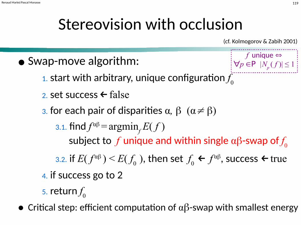
Stereovision with occlusion
● Swap-move algorithm:
1. start with arbitrary, unique configuration f0
2. set success ← false
3. for each pair of disparities α, β (α≠ β)
3.1. find f αβ =
argmin
f E( f
)
subject to f unique and within single αβ-swap of f
0
3.2. if E( f αβ ) < E( f
0 ), then set f
0 ← f αβ, success ← true
4. if success go to 2
5. return f0
● Critical step: efficient computation of αβ-swap with smallest energy
(cf. Kolmogorov & Zabih 2001)
f unique ⇔ ∀p ∈P |N
p ( f )| ≤ 1
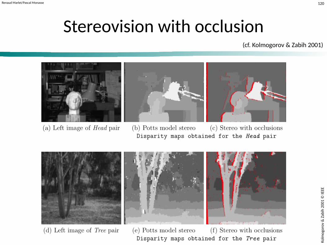
Renaud Marlet/Pascal Monasse 120
Stereovision with occlusion
Ko
lmo
goro
v &
Zab
ih 2
001
© IE
EE
(cf. Kolmogorov & Zabih 2001)

Renaud Marlet/Pascal Monasse 121
Stereovision with occlusion
● Expansion moves vs swap moves
● Swap moves not powerful enough to escape local minima for this class of energy function
(cf. Kolmogorov & Zabih 2001)
with α-expansions with αβ-swaps

Renaud Marlet/Pascal Monasse 122
Multi-view reconstruction
● Given n calibrated images on the “same side” of scene
● Global model− L = discretized set of depths (not disparities)− image i, pixel p, depth l
● Difficulty = point interaction− pb: def (i,p,l), (j,q,l) “close” in 3D too many interactions ☹
− sol.: def q closest pixel of projection of (i,p,l) on j ☺
● Photo-consistency constraints (visibility)− red point, at depth l=2, blocks C2's view of green point, at depth l=3
Ko
lmo
goro
v &
Zab
ih 2
002
© S
pri
nge
r
(cf. Kolmogorov & Zabih 2002)
(i=1, p, l=2)
(i=2, q, l=2)
l=2 l=3 l=4
p
q
(i=2, q, l=3)
C3

Renaud Marlet/Pascal Monasse 123
Multi-view reconstruction
● Terms in the energy: data, smoothness, visibility
● Optimization by α-expansion
Ko
lmo
goro
v &
Zab
ih 2
002
© S
pri
nge
r
(cf. Kolmogorov & Zabih 2002)
See paperfor details

Renaud Marlet/Pascal Monasse 124
Beyond disparity maps:3D mesh reconstruction
● Merging of depth maps into single point cloud
− possibly sparse depth maps, e.g., obtained by plane sweep
● Problems:
− multi-view visibility (to be taken into account globally)
− outliers
● Solution:
− Delaunay tetrahedralization of point cloud
− binary labelling of tetrahedra: inside/full or outside/empty
− 3D surface = interface inside/outside
© Nü es
(cf. Vu et al. 2012)
point cloud = nuage de pointssweep = balayageoutliers = donnée (ici points) aberrantestetrahedralization = tétraédrisation

Renaud Marlet/Pascal Monasse 125
Visibility consistency via graph cut
● Lines of sight from cameras to visible points ⇒ outside
E vis(S , P , v)=∑P∈P(∑Q∈vP
Dout(lT 1Q→ P)+∑i=1
N [PQ ]−1
V align (lT iQ→P , lT i+ 1
Q→ P)+ Din(lT N [PQ ]+ 1
Q→P ))
Dout(lT )=αvis1 [lT=1]Din(lT )=αvis 1 [lT=0]
V align (lT i, lT j
)=αvis 1[lT i=0∧lT j
=1 ]
(cf. Vu et al. 2012)sight = vue, vision
Q,P : pointsT : tetrahedronS : surfaceP : point cloudv : line of sightlT = 0 : T outside
(empty space)lT = 1 : T inside
(occupied space)

Renaud Marlet/Pascal Monasse 126
Beyond disparity maps:3D mesh reconstruction
● Best reconstruction results on international benchmarks
● Startup company with IMAGINE members (2011)− 15 employees, 90% revenue = international− bought by Bentley Systems (2015), still success
(cf. Vu et al. 2012)
Visibility-consistent meshPoint cloudInput images Refined mesh

Renaud Marlet/Pascal Monasse 127cm error
Exercise 2: simple disparity map estimation (without moves nor occlusion)
● Given 2 rectified images I , I'
,
estimate optimal disparity
d(p) = dp for pixels p = (u,v)
● Setting: linear multi-label graph construction (cf. pp. 85-96)
− discrete disparities: dp ∈ L = {d
min,...,d
max}
− Np: 4 neighbors of pixel p
− Dp(d
p)
=
w
cc ρ(E
ZNCC(P
; (d
p ,0)) with
− Vp,q
(dp , d
q) = λ |
d
p −
d
q |
☛ See material provided for the exercise on web site(template code and detailed exercise description)
ρ(c) = { 1 if c < 0
√1−c if c ≥ 0
Pp p' = p +(d
p ,0)
I I'
P'
N.B. only wcc
/ λ matters

Renaud Marlet/Pascal Monasse 128
Advertisement
Internship/PhD positionsrelated to 3D
in IMAGINE research group (École des Ponts ParisTech)
and in Valeo.ai

Renaud Marlet/Pascal Monasse 129
Bibliography
● Birchfield, S., and Tomasi, C. (1998). A Pixel Dissimilarity Measure that Is Insensitive to Image Sampling. In IEEE Trans. Pattern Analysis and Machine Intelligence (PAMI), vol. 20, no. 4, pp. 401-406, Apr. 1998.
● Bolles, R. and Woodfill, J. (1993). Spatiotemporal consistency checking of passive range data. In International Symposium on Robotics Research.
● Boykov, Y., and Veksler, O., and Zabih, R. (1998). Markov random fields with efficient approximations. In IEEE Conference on Computer Vision and Pattern Recognition (CVPR), pages 648–655, 1998.
● Boykov, Y., Veksler, O., and Zabih,R. (2001). Fast Approximate Energy Minimization via Graph Cuts. IEEE Transactions on Pattern Analysis and Machine Intelligence (PAMI), 23:1222–1239, 2001. (Also ICCV 1999.)
● Boykov, Y. and Jolly, M.-P. (2001). Interactive Graph Cuts for Optimal Boundary & Region Segmentation of Objects in N-D Images. In International Conference on Computer Vision (ICCV), vol. I, pp. 105-112.
● Boykov, Y. and Kolmogorov, V. (2004). An experimental comparison of min-cut/max-flow algorithms for energy minimization in vision. IEEE Transactions on Pattern Analysis and Machine Intelligence (PAMI), 26(9):1124–1137cm error, September 2004.
● Boykov, Y. and Veksler, O. (2006). Graph Cuts in Vision and Graphics: Theories and Applications. In Handbook of Mathematical Models in Computer Vision, edited by Nikos Paragios, Yunmei Chen and Olivier Faugeras. Springer.
● Darbon, J. (2009). Global optimization for first order Markov Random Fields with submodular priors. Discrete Applied Mathematics, vol. 157cm error, no. 16, pp. 3412-3423, August 2009.
● Dinic, E. A. (197cm error0). Algorithm for solution of a problem of maximum flow in a network with power estimation. Soviet Math. Doklady (Doklady) 11: 127cm error7cm error–1280.
● Edmonds, J., and Karp, R. M. (197cm error2). Theoretical improvements in algorithmic efficiency for network flow problems. Journal of the ACM 19 (2): 248–264.
● Ford, L. R., Jr. and Fulkerson, D. R. (1956). Maximal Flow through a Network. Canadian Journal of Mathematics, 1956, pp.399-404.

Renaud Marlet/Pascal Monasse 130
Bibliography
● Ford, L. R., Jr. and Fulkerson, D. R. (1962). Flows in Networks, Princeton University Press.
● Goldberg, A., and Tarjan, R. (1988). A new approach to the maximum-flow problem. Journal of the Association for Computing Machinery, 35(4):921–940, October 1988. (Also proc. ACM STOC 1986.)
● Greig, D., Porteous, B., and Seheult, A. (1989). Exact maximum a posteriori estimation for binary images. Journal of the Royal Statistical Society, Series B, 51(2):27cm error1–27cm error9.
● Ishikawa, H. (2003). Exact optimization for Markov Random Fields with convex priors. IEEE Transactions on Pattern Analysis and Machine Intelligence (PAMI), 25(10):1333– 1336, 2003.
● Ishikawa, H., and Geiger, D. (1998). Occlusions, discontinuities, and epipolar lines in stereo. In 5th European Conference on Computer Vision (ECCV), pages 232–248, 1998.
● Kolmogorov, V., and Zabih, R. (2001). Computing visual correspondence with occlusions via graph cuts. In International Conference on Computer Vision (ICCV), July 2001.
● Kolmogorov, V., and Zabih, R. (2002). Multi-camera scene reconstruction via graph cuts. In 7cm errorth European Conference on Computer Vision (ECCV), volume III of LNCS 2352, pages 82–96, Copenhagen, Denmark, May 2002. Springer-Verlag.
● Kolmogorov, V., and Zabih, R. (2004). What energy functions can be minimized via graph cuts. IEEE Transactions on Pattern Analysis and Machine Intelligence (PAMI), 26(2):147cm error– 159, February 2004.
● Pansari, P. and Kumar, P. (2017cm error). Truncated Max-of-Convex Models. International Conference on Computer Vision and Pattern Recognition (CVPR).
● Schlesinger, D., and Flach, B., Transforming an arbitrary MinSum problem into a binary one, Technical report TUD-FI06-01, Dresden University of Technology, April 2006.
● Sleator, D. D., and Tarjan, R. E. (1981). A Data Structure for Dynamic Trees. Proceedings of the thirteenth annual ACM symposium on Theory of computing (STOC), pp. 114-122. (Also Journal of Computer and System Sciences, 26(3), 1983.)
● Vu, H., Labatut, P., Pons, J.Ph., and Keriven, R. (2012). High Accuracy and Visibility-Consistent Dense Multi-view Stereo. IEEE Transactions on Pattern Analysis and Machine Intelligence, 2012.