Graph Edit Distance from Spectral Seriation

Antonio Robles-Kelly and Edwin R. Hancock ∗

Abstract

This paper is concerned with computing graph edit distance. One of the criticisms

that can be leveled at existing methods for computing graph edit distance is that they

lack some of the formality and rigour of the computation of string edit distance. Hence,

our aim is to convert graphs to string sequences so that string matching techniques

can be used. To do this we use a graph spectral seriation method to convert the ad-

jacency matrix into a string or sequence order. We show how the serial ordering can

be established using the leading eigenvector of the graph adjacency matrix. We pose

the problem of graph-matching as maximum a posteriori probability (MAP) alignment

of the seriation sequences for pairs of graphs. This treatment leads to an expression

in which the edit cost is the negative logarithm of the a posteriori sequence alignment

probability. We compute the edit distance by finding the sequence of string edit oper-

ations which minimise the cost of the path traversing the edit lattice. The edit costs

are determined by the components of the leading eigenvectors of the adjacency matrix,

and by the edge densities of the graphs being matched. We demonstrate the utility of

the edit-distance on a number of graph clustering problems.

1 Introduction

The quest for a robust means of inexact graph matching has been the focus of sustained

activity in the areas of computer vision and structural pattern recognition for over two

∗Department of Computer Science, The University of York, York, Y01 5DD, UK. email:

arobkell,erh@cs.york.ac.uk

1

decades [34, 31, 10, 12, 44, 26]. Many different approaches have been adopted to the problem,

including relaxation labelling [6, 11, 12, 44] and constraint satisfaction [35, 44, 4], structural

pattern recognition (including the use of graph edit distance) [31, 10], information theoretic

methods [26], and, graph-spectral methods [40, 22]. Each of these approaches has its merits.

For instance, information theoretic methods [6, 44] are strongly principled since they model

the graph-matching process using probability distributions. Matching by minimising edit

distance [31, 10, 26] is attractive since it gauges the similarity of graphs by counting the

number of structural modifications needed to make graphs isomorphic with one-another.

Graph spectral methods are elegant because of their use of a matrix representation [40, 22].

However, there are weaknesses too. Information theoretic methods are limited by the fact

that the required probability distributions can become difficult to construct and manipulate

due the combinatorial nature of the underlying state-space. Of course this problem can

be overcome to some extent by making simplifying assumptions. For instance, in relaxation

labelling the complexity can be curbed by representing the distribution over edges or faces [6].

In order to overcome the computational problems associated with using discrete densities,

Bagdanov and Worring [2] use normal distributions to model the distribution of the random

variables in their first-order Gaussian graphs. These methods can lead to algorithms for

learning graph prototypes from training data. In the case of graph edit-distance the costs of

elementary edit operations must be set heuristically since no well-defined learning procedure

exits, and moreover, the method lacks some of the formal underpinning of string edit distance.

Graph-spectral methods can be fragile to structural error [40] unless expensive iterative

methods are adopted [22].

The aim in this paper is to exploit some of the strengths of the methods listed above,

while overcoming their weaknesses. The overall aim is to use a spectral representation, and

to pose the computation of graph edit distance in a probabilistic setting. This work is timely

for a number of reasons. First, there has recently been renewed interest in the problem of

computing graph edit distance. For instance, Bunke and his co-workers have returned to

the problem and have shown a relationship between graph edit distance and the size of the

maximum common subgraph [3]. Second, graph spectral methods have been shown to work

2

effectively if either a careful choice of representation is made, or if they are combined with

statistical methods. For instance, Shokoufandeh et al [36] have shown how to index shock

trees using an eigenvalue interleaving theorem, and Luo and Hancock [22] have shown how

Umeyama’s [40] matrix factorisation method can be rendered robust to structural error using

the apparatus of the EM algorithm. However, despite this progress it is clear that there is

still much remaining to be done on the convergence of structural, spectral and statistical

methods.

1.1 Motivation

One way of overcoming the problems listed above is to use graph-spectral methods to convert

graphs to string sequences and to use probabilistic methods to measure the similarity of

the sequences, and hence compute graph edit distance. We have already performed an

initial study of this problem [29]. Here we made use of the relationship between the leading

eigenvector of the row-normalised adjacency matrix and the steady state random walk on

the associated graph. The string sequence is defined by the state probabilities of the random

walk after an infinite number of time steps. Edit distance computation is based on a set of

heuristic elementary costs. However, the string sequence delivered by the steady state site

probabilities is not guaranteed to be edge connected, and hence in comparing the strings

information concerning the structure of the graph is discarded. This paper takes this work

further by casting the problem of recovering an edge connected path sequence in a more

explicit energy minimisation setting, and, by casting the problems of computing edit costs

and string matching in a probabilistic setting.

To meet the goals listed above, in this paper we aim to recover a string in which the node

sequence order maximally preserves edge connectivity constraints. More specifically, we are

interested in the task of ordering the set of nodes in a graph in a sequence such that strongly

correlated nodes are placed next to one another. This problem is known as seriation and is

important in a number of areas including data visualisation and bioinformatics, where it is

used for DNA sequencing. The seriation problem can be approached in a number of ways.

Clearly the problem of searching for a serial ordering of the nodes, which maximally preserves

3

the edge ordering is one of exponential complexity. As a result approximate solution methods

have been employed. These involve casting the problem in an optimisation setting. Hence

techniques such as simulated annealing and mean field annealing have been applied to the

problem [33, 37]. It may also be formulated using semidefinite programming [17], which

is a technique closely akin to spectral graph theory since it relies on eigenvector methods.

However, recently Atkins, Boman and Hendrikson [1] have shown how to use an eigenvector

of the Laplacian matrix to sequence relational data. There is an obvious parallel between

this method and the use of eigenvector methods to locate steady state random walks on

graphs [25, 20].

Hence, we aim to exploit this seriation technique to develop a spectral method for com-

puting graph edit distance. The task of posing the inexact graph matching problem in a

matrix setting has proved to be an elusive one. This is disappointing since a rich set of po-

tential tools are available from the field of mathematics referred to as spectral graph theory.

This is the term given to a family of techniques that aim to characterise the global struc-

tural properties of graphs using the eigenvalues and eigenvectors of the adjacency matrix

[7]. In the computer vision literature there have been a number of attempts to use spectral

properties for graph-matching, object recognition and image segmentation. Umeyama has

an eigendecomposition method that matches graphs of the same size [40]. Borrowing ideas

from structural chemistry, Scott and Longuet-Higgins were among the first to use spectral

methods for correspondence analysis [32]. They showed how to recover correspondences

via singular value decomposition on the point association matrix between different images.

In keeping more closely with the spirit of spectral graph theory, Shapiro and Brady [35]

developed an extension of the Scott and Longuet-Higgins method, in which point sets are

matched by comparing the eigenvectors of the point proximity matrix. Horaud and Sossa

[15] have adopted a purely structural approach to the recognition of line-drawings. Their

representation is based on the immanental polynomials for the Laplacian matrix of the line-

connectivity graph. Shokoufandeh, Dickinson and Siddiqi [36] have shown how graphs can

be encoded using local topological spectra for shape recognition from large databases. In

a recent paper, Luo and Hancock [22] have returned to the method of Umeyama [40] and

4

have shown how it can be rendered robust to differences in graph-size and structural errors.

Commencing from a Bernoulli distribution for the correspondence errors, they develop an

expectation maximisation algorithm for graph-matching. Correspondences are recovered in

the M or maximisation step of the algorithm by performing singular value decomposition

on the weighted product of the adjacency matrices for the graphs being matched. The cor-

respondence weight matrix is updated in the E or expectation step. However, since it is

iterative the method is relatively slow and is sensitive to initialisation.

1.2 Contribution

We pose the recovery of the seriation path as that of finding an optimal permutation order

subject to edge connectivity constraints. By using the Perron-Frobenius theorem [41], we

show that the optimal permutation order is given by the leading eigenvector of the adja-

cency matrix. The seriation path may be obtained from this eigenvector using a simple

edge-filtering technique. By using the spectral seriation method, we are able to convert the

graph into a string. This opens up the possibility of performing graph matching by perform-

ing string alignment. We pose the problem as maximum a posteriori probability estimation

of an optimal alignment sequence on an edit lattice by minimising the Levenshtein or edit

distance [19, 42]. The edit distance is the negative log-likelihood of the a posteriori alignment

probability. To compute the alignment probability, we require two model ingredients. The

first of these is an edge compatibility measure for the edit sequence. We use a simple error

model to show how these compatibilities may be computed using the edge densities for the

graphs under match. The second model ingredient is a set of node correspondence prob-

abilities. We model these using a Gaussian distribution on the components of the leading

eigenvectors of the adjacency matrices. We can follow Wagner [42] and use dynamic pro-

gramming to evaluate the edit distance between strings and hence recover correspondences.

It is worth stressing that although there have been attempts to extend the string edit idea to

trees and graphs [31, 34], there is considerable current effort aimed at putting the underlying

methodology on a rigorous footing.

5

2 Graph Seriation

Consider the undirected graph G = (V, E) with node index-set V and edge-set E ⊆ V × V .

Associated with the graph is a symmetric adjacency matrix A whose elements are defined

as follows

A(j, k) =

1 if (j, k) ∈ E

0 otherwise

(1)

Our aim is to assign the nodes of the graph to a sequence order which preserves the edge

ordering of the nodes. This sequence can be viewed as an edge connected path on the graph.

Let the path commence at the node j1 and proceed via the sequence of edge-connected nodes

X = j1, j2, j3, ... where (ji, ji+1) ∈ E. With these ingredients, the problem of finding the

path can be viewed as one of seriation, subject to edge connectivity constraints.

The seriation problem as stated by Atkins, Boman and Hendrickson [1] is as follows.

The aim is to find a path sequence for the nodes in the graph using a permutation π. The

required permutation is sought so as to minimise the penalty function

g(π) =

|V |∑i=1

|V |∑j=1

A(i, j)(π(i)− π(j))2

Unfortunately, minimising g(π) is potentially NP complete due to the combinatorial nature

of the discrete permutation π. To overcome this problem, a relaxed solution is sought that

approximates the structure of g(π) using a vector ~x = (x1, x2, ....) of continuous variables xi.

Hence, the penalty function considered is

g(~x) =

|V |∑i=1

|V |∑j=1

A(i, j)(xi − xj)2

The value of g(~x) does not change if a constant amount is added to each of the components

xi. Hence, the minimisation problem must be subject to constraints on the components of

the vector ~x. The constraints are that

|V |∑i=1

x2i = 1 and

|V |∑i=1

x2i 6= 0 (2)

Atkins, Bowman and Atkinson show that the solution to this relaxed problem may be ob-

tained from the Fiedler vector of the Laplacian matrix L = D−A, where D is the diagonal

6

degree matrix with elements D(i, i) =∑|V |

j=1 A(i, j) equal to the total weight of the edges

connected to the node i.

Unfortunately, the procedure described above does not meet our requirements since the

penalty function g(~x), does not impose edge connectivity constraints on the ordering com-

puted during the minimisation process. To overcome this shortcoming, we turn our attention

instead to maximising the cost function

gE(~x) =

|V |−1∑i=1

|V |∑

k=1

(A(i, k) + A(i + 1, k))x2k (3)

When we combine the modified cost function with the constraints, we have that

|V |−1∑i=1

|V |∑

k=1

(A(i, k) + A(i + 1, k))x2k = λ

|V |−1∑i=1

(x2i + x2

i+1) (4)

By introducing the matrix

Ω =

1 0 0 0 . . . 0

0 2 0 0 . . . 0

0 0 2 0 . . . 0...

.... . . . . . . . .

...

0 0 . . . 0 2 0

0 0 . . . 0 0 1

(5)

we can make the path connectivity requirement more explicit, and the maximiser of gE(~x)

satisfies the condition

λ = arg maxx∗

~xT∗ΩA~x∗~xT∗Ω~x∗

(6)

As a result, the leading eigenvalue λ∗ of the adjacency matrix A is the maximiser of

the cost function gE(~x). ¿From the Perron-Frobenius theorem [41], it is known that the

maximiser of this utility function is the leading (left) eigenvector of the matrix A . More-

over, since A is a real positive definite symmetric matrix, the associated eigenvector φ∗ is

unique. The Perron-Frobenius theorem ensures that the maximum eigenvalue λ∗ > 0 of A

has multiplicity one and, moreover, the coefficients of the corresponding eigenvector φ∗ are

all positive. As a result the remaining eigenvectors of A have at least one negative coefficient

7

and one positive coefficient. If A is substochastic, φ∗ is also known to be linearly independent

of the all-ones vector e.

The elements of the leading eigenvector φ∗ can be used to construct a serial ordering of

the nodes in the graph. We commence from the node associated with the largest component

of φ∗. We then sort the elements of the leading eigenvector such that they are both in the de-

creasing magnitude order of the coefficients of the eigenvector, and satisfy edge connectivity

constraints on the graph. The procedure is a recursive one that proceeds as follows. At each

iteration, we maintain a list of nodes visited. At iteration k let the list of nodes be denoted

by Lk. Initially, L1 = j1 where j1 = arg maxj φ∗(j), i.e. j1 is the component of φ∗ with the

largest magnitude. Next, we search through the set of first neighbours Nj1 = k|(j1, k) ∈ Eof j1 to find the node associated with the largest remaining component of φ∗. The second

element in the list is j2 = arg maxl∈Nj1φ∗(l). The node index j2 is appended to the list of

nodes visited and the result is L2. In the kth (general) step of the algorithm we are at the

node indexed jk and the list of nodes visited by the path so far is Lk. We search through

those first-neighbours of jk that have not already been traversed by the path. The set of

nodes is Ck = l|l ∈ Njk∧ l /∈ Lk. The next site to be appended to the path list is therefore

jk+1 = arg maxl∈Ckφ∗(l). This process is repeated until no further moves can be made. This

occurs when Ck = ∅ and we denote the index of the termination of the path by T . The

serial ordering of the nodes of the graph X is given by the ordered list or string of node

indices LT . Hence, the path commences at the node with the highest ranked eigenvector

component, and then proceeds in an edge connected manner through the sequence of nodes

that minimise the difference in the components of the eigenvector.

Figure 1 illustrates the seriation method on a simple graph. The left-hand panel shows

the original graph with numeric labels assigned to the nodes. In the centre-panel we show

the components of the leading eigenvector of the adjacency matrix, ordered according the

numeric order of the node-labels. In the right-hand panel, we show the seriation path. This

commences at the centre of the graph, and then moves around the perimeter.

There are similarities between the use of the leading eigenvector for seriation and the

use of spectral methods to find the steady state random walk on a graph. There are more

8

1

2

3

4

5

6

7

0 1 2 3 4 5 6 7 80

0.05

0.1

0.15

0.2

0.25

0.3

0.35

0.4

0.45

0.5

Node Index

Eig

enve

ctor

Coe

ffici

ent

1

2

3

4

5

6

7

Figure 1: Left-hand panel: example graph; Middle panel: corresponding leading eigenvector;

Right-hand panel: seriation results.

detailed discussions of the problem of locating the steady state random walk on a graph in

the reviews by Lovasz [20] and Mohar [25]. An important result described in these papers,

is that if we visit the nodes of the graph in the order defined by the magnitudes of the

coefficients of the leading eigenvector of the transition probability matrix, then the path is

the steady state Markov chain. In a recent paper [29], which represents the starting point

which lead us to the research reported here, we have used the rank order of the steady state

node visitation probabilities to define a string order. However, this path is not guaranteed

to be edge connected. Hence, it can not be used to impose a string ordering on the nodes

of a graph that encompasses edge-constraints. The seriation approach adopted in this paper

does, on the other hand, impose edge connectivity constraints and can hence be used to

convert graphs to strings in a manner which is suitable for computing edit distance.

3 Probabilistic Framework

We are interested in computing the edit distance between the graphs GM = (VM , EM)

referred to as the model graph and the graph GD = (VD, ED) referred to as the data-

graph. The leading eigenvectors of the adjacency matrices AM for the graph GM and AD

for the graph GD are respectively φ∗M and φ∗D. The seriations of the two graphs generated

from the leading eigenvectors are denoted by X = x1, x2, ....., x|VM | for the model graph

and Y = y1, y2, ....., y|VD| for the data graph. These two strings are used to index the

9

rows and columns of an edit lattice. The rows of the lattice are indexed using the data-

graph string, while the columns are indexed using the model-graph string. To allow for

differences in the sizes of the graphs we introduce a null symbol ε which can be used to pad

the strings. We pose the problem of computing the edit distance as that of finding a path

Γ =< γ1, γ2, ...γk, ....., γL > through the lattice. Each element γk ∈ (VD ∪ ε) × (VM ∪ ε)

of the edit path is a Cartesian pair. We constrain the path to be connected on the edit

lattice. In particular, the transition on the edit lattice from the state γk to the state γk+1 is

constrained to move in a direction that is increasing and connected in the horizontal, vertical

or diagonal direction on the lattice. The diagonal transition corresponds to the match of

an edge of the data graph to an edge of the model graph. A horizontal transition means

that the data-graph index is not incremented, and this corresponds to the case where the

traversed nodes of the model graph are null-matched. Similarly when a vertical transition is

made, then the traversed nodes of the data-graph are null-matched.

Suppose that γk = (a, b) and γk+1 = (c, d) represent adjacent states in the edit path

between the seriations X and Y . According to the classical approach [42], the cost of the

edit path is given by the sum of the costs of the elementary edit operations

d(X, Y ) = C(Γ) =∑γk∈Γ

η(γk → γk+1) (7)

where η(γk → γk+1) is the cost of the transition between the states γk = (a, b) and γk+1 =

(c, d). The optimal edit path is the one that minimises the edit distance between the strings,

and satisfies the condition Γ∗ = arg minΓ C(Γ), and the edit distance is d(X,Y ) = C(Γ∗).

Classically, the optimal edit sequence may be found using Dijkstra’s algorithm [8] or by

using the quadratic programming method of Wagner and Fisher [42]. However, there are

two reasons why the classical string edit distance does not meet our needs in this paper.

First, the edit costs need to reflect the string encoding of graph structure. In other words,

the transitions on the edit lattice must take into account whether edge structure is being

matched in a consistent manner. Second, we would like to cast the problem of minimum edit

distance matching in a probabilistic setting so that we can develop statistical models for the

costs on the edit lattice. In particular, we would like to do this in a manner which separates

10

the costs of visiting individual sites on the lattice and of making transitions between sites. In

this way we can separate the role of evidence, i.e. the components of the leading eigenvectors,

and constraints, i.e. whether edges are matched consistently.

Rather than commencing from an expression for the edit-cost, in this paper we pose the

problem of recovering the optimal edit sequence as one of maximum a posteriori probability

estimation. We aim to find the edit path that has maximum probability given the available

leading eigenvectors of the data-graph and model-graph adjacency matrices. Hence, the

optimal path is the one that satisfies the condition Γ∗ = arg maxΓ P (Γ|φ∗X , φ∗Y ).

To develop this decision criterion into a practical edit distance computation scheme, we

need to develop the a posteriori probability appearing above. We commence by using the

definition of conditional probability to re-write the a posteriori path probability in terms

of the joint probability density P (φ∗X , φ∗Y ) for the leading eigenvectors and the joint density

function P (φ∗X , φ∗Y , Γ) for the leading eigenvectors and the edit path. The result is

P (Γ|φ∗X , φ∗Y ) =P (φ∗X , φ∗Y , Γ)

P (φ∗X , φ∗Y )(8)

We can rewrite the joint density appearing in the numerator to emphasise and make

explicit both the role of the components of the adjacency matrix leading eigenvectors and

the component edit transitions. In this form

P (Γ|φ∗X , φ∗Y ) =P (φ∗X(1), φ∗X(2), ...., φ∗Y (1), φ∗Y (2), ..., γ1, γ2, ...)

P (φ∗X , φ∗Y )(9)

To simplify the numerator, we make a conditional independence assumption. Specifically,

we assume that the components φ∗X(a) and φ∗Y (b) of the leading eigenvectors of the model

and data-graph adjacency matrices, depend only on the edit transition γk = (a, b) associated

with their node-indices. Using the chain-rule for conditional probability we can perform the

factorisation

P (φ∗X(1), φ∗X(2), ...., φ∗Y (1), φ∗Y (2) . . . , γ1, γ2, ...)

P (φ∗X , φ∗Y )=

L∏

k=1

P (φ∗X(a), φ∗Y (b)|γk)

P (γ1, γ2, . . . , γL)

and as a result

P (Γ|φ∗X , φ∗Y ) =

∏Lk=1 P (φ∗X(a), φ∗Y (b)|γk)

P (γ1, γ2, . . . , γL)

P (φ∗X , φ∗Y )(10)

11

where P (γ1, γ2, ..., γL) is the joint prior for the sequence of edit transitions. To simplify the

joint prior, we commence by applying the chain-rule of conditional probability

P (γ1, γ2, . . . , γL) = P (γ1|γ2, . . . , γL)P (γ2|γ3, . . . , γL) . . . P (γk|γk+1, . . . , γL) . . . P (γL−1|γL)P (γL)

(11)

To simplify this factorisation we assume that the sites on the edit lattice are conditionally

dependant only on those that are immediate neighbours. As a result P (γk|γk+1, . . . , γL) =

P (γk|γk+1). Hence, we can write

P (γ1, γ2, . . . , γL) = P (γL)L−1∏

k=1

P (γk|γk+1) (12)

This takes the form of a factorisation of conditional probabilities for transitions between

sites on the edit lattice P (γk|γk+1), except for the term P (γL) which results from the final

site visited on the lattice. To arrive at a more homogeneous expression, we use the definition

of conditional probability to re-express the joint conditional measurement density for the

adjacency matrix leading eigenvectors in the following form

P (φ∗X(a), φ∗Y (b)|γk) =P (γk|φ∗X(a), φ∗Y (b))P (φ∗X(a), φ∗Y (b))

P (γk)(13)

Substituting Equations (12) and (13) into Equation (10) we find

P (Γ|φ∗X , φ∗Y ) =

L∏

k=1

P (γk|φ∗X(a), φ∗Y (b))P (γk, γk+1)

P (γk)P (γk+1)

∏Lk=1 P (φ∗X(a), φ∗Y (b))

P (φ∗X , φ∗Y )

Since, the joint measurement density P (φ∗X , φ∗Y ) does not depend on the edit path, it

does not influence the decision process, and we remove it from further consideration. Hence,

the optimal path across the edit lattice is

Γ∗ = arg maxγ1,γ2...,γL

L∏

k=1

P (γk|φ∗X(a), φ∗Y (b))P (γk, γk+1)

P (γk)P (γk+1)

(14)

The information concerning the structure of the edit path on the lattice is captured by

the quantity

Rk,k+1 =P (γk, γk+1)

P (γk)P (γk+1)(15)

12

We refer to this quantity as the edge-compatibility coefficient.

To establish a link with the classical edit distance picture presented earlier, we can re-

express the location of the optimal edit path as an minimisation problem involving the

negative logarithm of the a posteriori path probability. The optimal path is the one that

satisfies the condition

Γ∗ = arg minγ1,γ2...,γL

L∑

k=1

[− ln P (γk|φ∗X(a), φ∗Y (b))− ln Rk,k+1

](16)

As a result the elementary edit cost η(γk → γk+1) associated with the transition from the

site γk = (a, b) to the site γk+1 = (c, d) is

η(γk → γk+1) = −(ln P (γk|φ∗X(a), φ∗Y (b)) + ln P (γk+1|φ∗X(c), φ∗Y (d)) + ln Rk,k+1

)(17)

The expression hence contains separate terms associated with the cost of visiting indi-

vidual sites on the lattice, and for making transitions between sites. The cost of visiting the

sites depends only on the components of the eigenvectors, and reflects the raw measurement

data available to the graph matching method. The transition between sites, on the other

hand, depends on whether there is consistent connecting edge structure between the sites on

the edit lattice.

4 Model Ingredients

To compute the edit costs, we require models of the a posteriori probabilities of visiting the

sites of the edit lattice, i.e. P (γk|φ∗X(a), φ∗Y (b)) and of Rk,k+1.

4.1 Lattice Transition Probabilities

The edge compatibility coefficient Rk,k+1 can be modelled using a simple model of node

attendance [43]. We assume that there is a uniform probability p that individual nodes, in

either of the graphs being matched, are missing due to the action of detection errors. These

errors may be due to a number of processes including imperfections in the image segmentation

process or occlusions. We assume that the detection errors operate independently on the

13

nodes of the graphs. As a result uncorrupted edges occur with total probability mass (1−p)2.

This probability mass is distributed between the |E| edges of the graph. Edges with one

node present and one-node missing have total probability mass 2p(1 − p). This probability

mass is distributed amongst the 2|V | configurations involving a node and a null-symbol ε.

Edges in which both nodes are missed take the remaining probability mass, i.e. p2. There is

one such configuration i.e. (ε, ε) to which this mass of probability may be assigned.

When the two graphs to be matched are considered together, then there are nine cases

in which the assigned probability is non-zero. We assume that joint errors in the two graphs

under consideration are independent. Hence, the probabilities are taken in product. If pM

and pD are the node detection error probabilities for the model and data graphs, then the

distribution of joint probability for the transitions on the edit lattice is specified by the

following rule

P (γk, γk+1) =

(1−pD)2

|ED|(1−pM )2

|EM | if (a, c) ∈ ED and (b, d) ∈ EM

(1−pD)2

|ED|pM (1−pM )

|VM | if (a, c) ∈ ED and (b, d) ∈ (VM × ε) ∪ (ε× VM)

(1−pD)2

|ED| p2M if (a, c) ∈ ED and (b, d) = (ε, ε)

pD(1−pD)|VD|

(1−pM )2

|EM | if (a, c) ∈ (VD × ε) ∪ (ε× VD) and (b, d) ∈ EM

pD(1−pD)|VD|

pM (1−pM )|VM | if (a, c) ∈ (VD × ε) ∪ (ε× VD) and (b, d) ∈ (VM × ε) ∪ (ε× VD)

pD(1−pD)|VD| p2

M if (a, c) ∈ (VD × ε) ∪ (ε× VD) and (b, d) = (ε, ε)

p2D

(1−pM )2

|VM | if (a, c) = (ε, ε) and (b, d) ∈ EM

p2D

pM (1−pM )|VM | if (a, c) = (ε, ε) and (b, d) ∈ (VM × ε) ∪ (ε× VM)

p2Dp2

M if (a, c) = (ε, ε) and (b, d) = (ε, ε)

0 otherwise

(18)

The single-site priors are found by summing the joint priors i.e. P (γk) =∑

γk+1P (γk, γk+1),

14

and are given by

P (γk) =

(1−pD)|VD|

(1−pM )|VM | if a ∈ VD and b ∈ VM

(1−pD)|VD| pM if a ∈ VD and b = ε

pD(1−pM )|VM | if a = ε and b ∈ VM

pDpM if a = ε and b = ε

(19)

As a result of these distribution rules, and under the assumption that the error process acts

independently in the two graphs being matched, it can be shown that the quantity Rk,k+1

depends only of the edge densities ρD = |VD|2ED

and ρM = |VM |2EM

for the two graphs under study.

The contingency table given can be expressed in terms of the transitions on the edit lattice.

The move contingency table is

Rk,k+1 =

ρMρD if γk → γk+1 is a diagonal transition on the edit lattice,

i.e. (a, c) ∈ ED and (b, d) ∈ EM

ρM if γk → γk+1 is a horizontal transition on the edit lattice,

i.e. (a, c) ∈ ED and b = ε or d = ε

ρD if γk → γk+1 is a vertical transition on the edit lattice,

i.e. a = ε or c = ε and (b, d) ∈ EM

1 if a = ε or c = ε and b = ε or d = ε

(20)

The node detection probabilities are cancelled-out between the numerator and denominator,

and as a result the edge-compatibility coefficients are determined only by the edge densities

in the two graphs being matched.

4.2 A Posteriori Correspondence Probabilities

The second model ingredient is the a posteriori probability of visiting a site on the lattice.

To motivate our model, we draw on matrix perturbation theory [38]. It can be shown that

the change in the leading eigenvector depends in a linear manner on the perturbations in

the elements of the adjacency matrix [30]. Moreover, in prior work, we have shown that a

Bernoulli distribution can be successfully used to model noise in the elements of the adjacency

15

matrix [28]. As a result, if the matrix is large (i.e. the change in the leading eigenvector

is the result of the sum of a large number of adjacency matrix element perturbations),

then, as a consequence of the central limit theorem, the distribution of errors in the leading

eigenvector due to perturbations in the elements of the adjacency matrix will be Gaussian.

In other words we can write,

P (γk|φ∗X(a), φ∗Y (b)) =

1√2πσ

exp

− 1

2σ2 (φ∗X(a)− φ∗Y (b))2

if a 6= ε and b 6= ε

α if a = ε or b = ε

(21)

where σ2 is the noise variance for the components of the leading eigenvectors. The perturba-

tion argument does not deal with the more intractable problem of modelling changes in the

size of the matrix (i.e. possible node insertions and deletions). In addition, it is worth men-

tioning that there are alternatives to measuring the difference in the eigenvectors using the

L2 norm between eigenvectors in the probability distribution function. For instance, error

could be measured by the angle between eigenvectors making use of a Von Mises distribution

[24].

4.3 Minimum Cost Path

Once the edit costs are computed, we proceed to find the path that yields the minimum

edit distance. Our adopted algorithm makes use of the fact that the minimum cost path

along the edit lattice is composed of sub-paths that are also always of minimum cost. Hence,

following Levenshtein [19] we compute a |VD| × |VM | transition-cost matrix ψ. The elements

of the matrix are computed recursively using the formula

ψ(i, j) =

η(γi → γj) if j = 1 and i = 1

η(γi → γj) + ψi,j−1 if i = 1 and j ≥ 2

η(γi → γj) + ψi−1,j if j = 1 and i ≥ 2

η(γi → γj) + min(ψi−1,j, ψi,j−1, ψi−1,j−1) if i ≥ 2 and j ≥ 2

(22)

The matrix ψ is a representation of the accumulated minimal costs of the path along

the edit lattice constrained to horizontal, vertical and diagonal transitions between adjacent

16

Figure 2: Example images and associated Delaunay triangulations.

coordinates. The minimum cost path can be proven to be that of the path closest to the

diagonal of the matrix [19]. As a result, the edit distance is given by the bottom rightmost

element of the transition-cost matrix. Hence, d(X, Y ) = ψ(|VD|, |VM |).At this point it is worth commenting on the complexity of the seriation method. First, the

leading eigenvector of the adjacency matrix needs to be computed. For a N ×N adjacency

matrix, there are numerical methods that can recover the eigenvalues and eigenvectors with

complexity O(N3). However, the leading eigenvector can be computed with complexity

O(N2) using the power method [13]. Second, we need to search for the seriation path of the

average degree of the graph is D, then the cost of this step is O(N(D − 1)). Finally, the

minimum cost edit path needs to recovered. If the longer string being matched is of length

N and the shorter one of length M , then the complexity of this step is O(NM2).

5 Experiments

Our experimental study is concerned with demonstrating the utility of the distances com-

puted using our new method for the problem of graph-clustering. We explore three real-world

problems. The first of these involves a database containing different views of a number of

3D objects. The second application involves view-based object recognition from 2D views

of 3D objects using topographic information furnished using shape-from-shading. The third

17

problem involves finding sets of similar shapes in a database of trademarks and logos 1.

5.1 View-based Object Recognition

We have experimented with our new matching method on an application involving a database

containing different perspective views of a number of 3D objects. The objects used in our

study are model houses. The different views are obtained as the camera circumscribes the

object. The three object sequences used in our experiments are the CMU-VASC sequence,

the INRIA MOVI sequence and a sequence of views of a model Swiss chalet. In our experi-

ments we use ten images from each of the sequences. To construct graphs for the purposes of

matching, we have first extracted corners from the images using the corner detector of Luo,

Cross and Hancock [21]. The graphs used in our experiments are the Delaunay triangula-

tions of these corner points. Our reason for using the Delaunay graph, is that of the point

neighbourhood graphs (k-nearest neighbour graph, Gabriel graph, relative neighbourhood

graph) it is the one that is least sensitive to node deletion errors [39]. Example images from

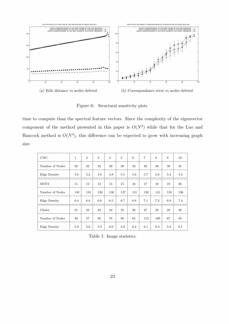
the sequences and their associated Delaunay are shown in Figure 2. In Table 1 we list the

numbers of nodes in the graphs and their edge densities. The table is divided into three

blocks. Each block is for a different image sequence. The top row in each block shows the

sequence number for the images.

5.1.1 Clustering

For the 30 graphs contained in the database, we have computed the complete set of 30 ×29 =870 distances between each of the distinct pairs of graphs. We compare our results

with those obtained when using the distances computed using two alternative methods.

The first of these is the negative log-likelihood function computed using the EM algorithm

reported by Luo and Hancock [22]. In this work the similarity of the graphs is gauged by the

quantity Tr[ATDQMQT ] where AD is the |VD|×|VD| data-graph adjacency matrix, AM is the

|VM | × |VM | model graph adjacency matrix and Q is a |VD| × |VD| matrix of correspondence

1All trademarks and logotypes remain the property of their respective owners. All trademarks and registered trademarks

are used strictly for educational and academic purposes and without intent to infringe on the mark owners.

18

10

20

30

40

50

60

70

80

90

100

5 10 15 20 25 30

5

10

15

20

25

30

(a)

0

50

100

150

200

250

5 10 15 20 25 30

5

10

15

20

25

30

(b)

0

50

100

150

200

250

5 10 15 20 25 30

5

10

15

20

25

30

(c)

Figure 3: Edit distance matrices.

probabilities between the nodes of the data-graph and the model-graph. Maximum likelihood

matches are found by performing singular value decomposition on the weighted correlation

matrix ATDQAM between the data-graph adjacency matrix and the model-graph adjacency

matrix. This similarity measure uses purely structural information. The method hence shares

with our edit distance framework the use of a statistical method to compare the eigenvector

structure of two adjacency matrices. However, unlike our method which uses only the leading

eigenvector of the adjacency matrix, this method uses the full pattern of singular vectors. In

addition, the method is an iterative one which alternates between computing singular vectors

in the M or maximisation step and re-computing the correspondence probability matrix Q in

the E or expectation step. The second of the distance measures is computed using a spectral

embedding of the graphs [23]. The method involves embedding the graphs in a pattern space

spanned by the leading eigenvalues of the adjacency matrix. According to this method, the

distance between graphs is simply the L2 norm between points in this pattern space [23].

This pairwise graph similarity measure again shares with our new method the feature of

using spectral properties of the adjacency matrix.

In Figure 3a we show the distance matrix computed using our algorithm. The similarity

matrix obtained using the method of Luo and Hancock [23] is shown in Figure 3b, while

the distance matrix computed from the spectral embedding is shown in Figure 3c. In each

distance-matrix the element with row column indices i, j corresponds to the pairwise similar-

ity between the graph indexed i and the graph indexed j in the database. In each matrix the

19

graphs are arranged so that the row and column index increase monotonically with viewing

angle. The blocks of views for the different objects follow one another. The darker the entry,

the smaller the distance. From the matrices in Figure 3, it is clear that the different objects

appear as distinct blocks. Within each block, there is substructure (sub-blocks) which cor-

respond to different characteristic views of the object. The main feature to note from the

three matrices is that there is less confusion between the third block (Chalet sequence) and

the first two blocks (CMU and MOVI sequences), when our edit-distance method is used.

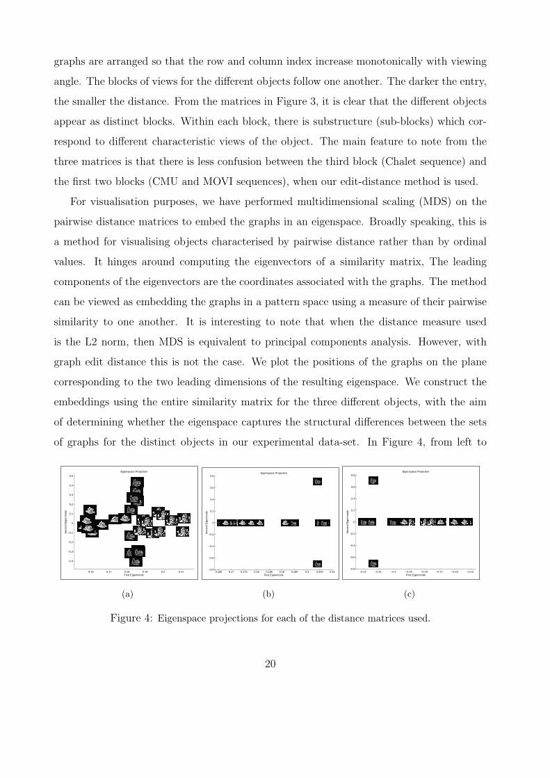
For visualisation purposes, we have performed multidimensional scaling (MDS) on the

pairwise distance matrices to embed the graphs in an eigenspace. Broadly speaking, this is

a method for visualising objects characterised by pairwise distance rather than by ordinal

values. It hinges around computing the eigenvectors of a similarity matrix, The leading

components of the eigenvectors are the coordinates associated with the graphs. The method

can be viewed as embedding the graphs in a pattern space using a measure of their pairwise

similarity to one another. It is interesting to note that when the distance measure used

is the L2 norm, then MDS is equivalent to principal components analysis. However, with

graph edit distance this is not the case. We plot the positions of the graphs on the plane

corresponding to the two leading dimensions of the resulting eigenspace. We construct the

embeddings using the entire similarity matrix for the three different objects, with the aim

of determining whether the eigenspace captures the structural differences between the sets

of graphs for the distinct objects in our experimental data-set. In Figure 4, from left to

0.16 0.17 0.18 0.19 0.2 0.21

−0.4

−0.3

−0.2

−0.1

0

0.1

0.2

0.3

0.4

0.5

First Eigenmode

Sec

ond

Eig

enm

ode

Eigenspace Projection

(a)

0.165 0.17 0.175 0.18 0.185 0.19 0.195 0.2 0.205 0.21−0.8

−0.6

−0.4

−0.2

0

0.2

0.4

0.6

0.8

First Eigenmode

Sec

ond

Eig

enm

ode

Eigenspace Projection

(b)

−0.22 −0.21 −0.2 −0.19 −0.18 −0.17 −0.16 −0.15−0.8

−0.6

−0.4

−0.2

0

0.2

0.4

0.6

0.8

First Eigenmode

Sec

ond

Eig

enm

ode

Eigenspace Projection

(c)

Figure 4: Eigenspace projections for each of the distance matrices used.

20

right, we show the embeddings corresponding to the distance matrices computed using our

algorithm, the negative log-likelihood computed using the algorithm of Luo and Hancock

[23] and the spectral feature-vectors extracted from the adjacency matrix [23]. Of the three

distance measures, the clusters resulting from the use of the edit distance described in this

paper produce the clearest cluster structure. Hence our new distance measure appears to be

effective at distinguishing between different classes of object.

Based on the visualisation provided by MDS, it appears that the distances furnished

by our edit-distance method may be suitable for the purposes of graph-clustering. We

have therefore applied a pairwise clustering algorithm to the similarity data for the graphs.

The process of pairwise clustering is somewhat different to the more familiar one of central

clustering. Whereas central clustering aims to characterise cluster-membership using the

cluster mean and variance, in pairwise clustering it is the relational similarity of pairs of

objects which are used to establish cluster membership. Although less well studied than

central clustering, there has recently been renewed interest in pairwise clustering aimed

at placing the method on a more principled footing using techniques such as mean-field

annealing [14]. In this paper we apply the pairwise clustering algorithm of Robles-Kelly

and Hancock [28] to the similarity data for the complete database of graphs. Our aim is

to determine which distance measure results in a cluster assignment which best corresponds

to the three image sequences. The pairwise clustering algorithm requires distances to be

represented by a matrix of pairwise affinity weights. Ideally, the smaller the distance, the

stronger the weight, and hence the mutual affinity to a cluster. The affinity weights are

required to be in the interval [0, 1]. For the pair of graphs indexed i1 and i2 the affinity

weight is taken to be

W(0)i1,i2 = exp

(−kd(i1, i2)

maxi1,iq(d(il, iq))

)(23)

where k is a constant and d(i1, i2) is the edit distance between the graph indexed i1 and the

graph indexed i2. The clustering algorithm is described in detail in [28] and is summarised

in the supplementary electronic material. It is an iterative process. The process maintains

two sets of variables. The first of these is a set of cluster membership indicators s(n)iω which

measures the affinity of the graph indexed i to the cluster indexed ω at iteration n of the

21

0

0.1

0.2

0.3

0.4

0.5

0.6

0.7

0.8

0.9

1

5 10 15 20 25 30

5

10

15

20

25

300

0.1

0.2

0.3

0.4

0.5

0.6

0.7

0.8

0.9

1

5 10 15 20 25 30

5

10

15

20

25

300

0.1

0.2

0.3

0.4

0.5

0.6

0.7

0.8

0.9

1

5 10 15 20 25 30

5

10

15

20

25

30

Figure 5: Final similarity matrices for the clustering process.

algorithm. The second, is an estimate of the affinity matrix based on the current cluster-

membership indicators W (n). These two sets of variables are estimated using interleaved

update steps, which are formulated to maximise a likelihood function for the pairwise cluster

configuration.

The final similarity matrices generated by the clustering process for each of the distance

measures studied are shown in Figure 5. From left-to-right, the panels show the similarity

matrices obtained using our edit distance, the Luo and Hancock structural graph matching

algorithm (SGM), and the spectral feature vectors. The lighter the entries, the more similar

the corresponding pairs of graphs. Ideally, the clusters should appear as square blocks centred

along the diagonal of the matrices. The misassignment of graphs to clusters is characterised

by strong response outside these blocks. In the case of our edit distance, the first and

seventh graphs in the third block (i.e. the Chalet sequence) are respectively misassigned to

the first block (the CMU sequence) and the second block (the MOVI sequence). In the case

of the spectral feature vectors, four of the Chalet sequence graphs are misassigned to the

MOVI sequence. In the case of Luo and Hancock method, only the seventh Chalet graph is

misassigned to the MOVI cluster. The errors are due to the fact that the graphs in question

are morphologically more similar to the graphs in the CMU and MOVI sequences than to

those in the Chalet sequence. Our method compares favourably when computational cost

is taken into account. This is because our method only requires the computation of the

leading eigenvector while the spectral feature vectors require the complete eigenstructure

to be computed. In consequence, the edit distance takes on average a factor of 2.6 less

22

0

50

100

150

200

0 20 40 60 80 100

EDIT DISTANCE AS A FUNCTION OF THE PERCENTAGE OF NODES DELETED

GRAPH CORRESPONDING TO THE FIRST FRAME OF THE CMU SEQUENCEGRAPH CORRESPONDING TO THE FIRST FRAME OF THE MOVI SEQUENCE

GRAPH CORRESPONDING TO THE FIRST FRAME OF THE CHALET SEQUENCE

(a) Edit distance vs nodes deleted

0

20

40

60

80

100

0 20 40 60 80 100

FRACTION OF INCORRECT CORRESPONDANCES VS PERCENTAGE OF NODES DELETED

GRAPH CORRESPONDING TO THE FIRST FRAME OF THE CMU SEQUENCEGRAPH CORRESPONDING TO THE FIRST FRAME OF THE MOVI SEQUENCE

GRAPH CORRESPONDING TO THE FIRST FRAME OF THE CHALET SEQUENCE

(b) Correspondance error vs nodes deleted

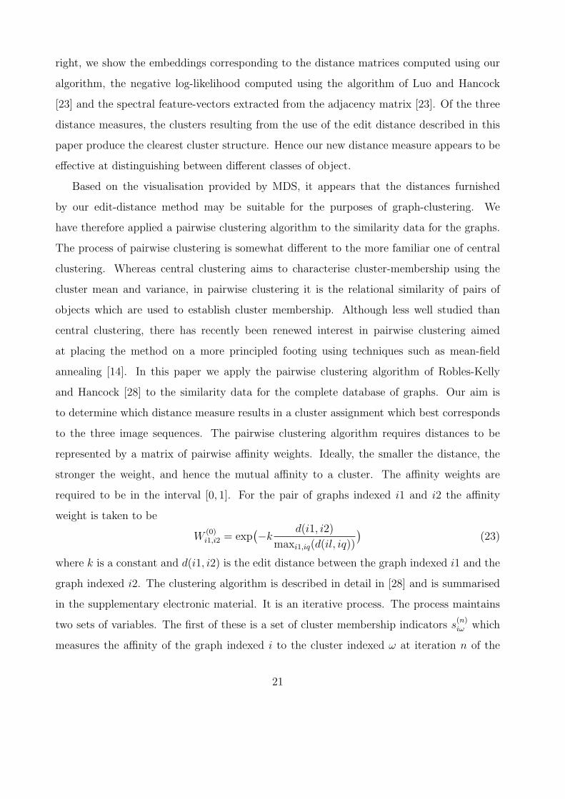
Figure 6: Structural sensitivity plots

time to compute than the spectral feature vectors. Since the complexity of the eigenvector

component of the method presented in this paper is O(N2) while that for the Luo and

Hancock method is O(N3), this difference can be expected to grow with increasing graph

size.

CMU 1 2 3 4 5 6 7 8 9 10

Number of Nodes 30 32 32 30 30 32 30 30 30 31

Edge Density 5.6 5.2 4.9 4.8 5.5 5.6 5.7 5.6 5.4 5.4

MOVI 11 12 13 14 15 16 17 18 19 20

Number of Nodes 140 134 130 136 137 131 139 141 133 136

Edge Density 6.4 6.8 6.6 6.5 6.7 6.8 7.1 7.2 6.9 7.4

Chalet 21 22 23 24 25 26 27 28 29 30

Number of Nodes 40 57 92 78 90 64 113 100 67 59

Edge Density 5.9 5.6 5.9 6.0 5.9 6.2 6.1 6.3 5.9 6.1

Table 1: Image statistics.

23

5.1.2 Structural Sensitivity to Node Deletion Error

We have conducted some experiments to measure the sensitivity of our matching method

to structural differences in the graphs and to provide comparison with alternatives. Here

we have taken the first graph from each of the three sequences described above. We have

simulated the effects of structural errors by randomly deleting nodes and re-triangulating

the remaining point-set. To demonstrate the effect of these structural errors, in Figure 6a

we show the edit distance as a function of the number of deleted nodes. We have averaged

the edit distance over 10 different sets of random node deletions. The different curves in the

plot are for the different seed graphs. In each case the edit distance varies almost linearly

with the number of deleted nodes. The deviations from the linear dependence occur when

large fractions of the graph are deleted.

To investigate the effect of node detection errors, in Figure 6b we show the fraction

of correspondence errors as a function of the fraction of nodes deleted from the graphs.

Here, we consider the model graph to be the initial graph, i.e. the deletion-free Delaunay

triangulation. The main features to note from this plot are as follows. First, the fraction

of correspondence errors is always lower than the fraction of deleted nodes. Second, there

appears to be no systematic effect of varying the graph size.

Finally, we investigated the effect of the node deletion errors on the results of MDS. In

Figure 7 we show the distance matrix (left-hand panel) and the MDS embedding (right-

hand panel) for the graphs. The graphs belonging to the different noise perturbed sets are

denoted by different characters, and form well defined clusters. Hence, structural (node

deletion errors) do not appear to affect adversely the clustering process.

5.2 Constant Shape Index Maximal Patches

Our second real world example is also concerned with view-based object recognition. Here we

have used the COIL database which consists of a series of 2D views of 3D objects collected at

72 equally spaced viewing directions on a great circle of the object view-sphere. To extract

graphs from the object-views, we have proceeded as follows. We first apply shape-from-

shading [45] to the object views to extract fields of surface normals. From the fields of surface

24

0

50

100

150

200

250

300

5 10 15 20 25 30

5

10

15

20

25

30 −0.23 −0.22 −0.21 −0.2 −0.19 −0.18 −0.17 −0.16 −0.15 −0.14−0.2

−0.15

−0.1

−0.05

0

0.05

0.1

0.15

0.2

0.25

0.3

First Eigenmode

Sec

ond

Eig

enm

ode

Eigenspace Projection

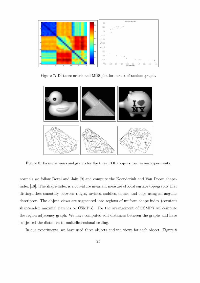
Figure 7: Distance matrix and MDS plot for our set of random graphs.

Figure 8: Example views and graphs for the three COIL objects used in our experiments.

normals we follow Dorai and Jain [9] and compute the Koenderink and Van Doorn shape-

index [18]. The shape-index is a curvature invariant measure of local surface topography that

distinguishes smoothly between ridges, ravines, saddles, domes and cups using an angular

descriptor. The object views are segmented into regions of uniform shape-index (constant

shape-index maximal patches or CSMP’s). For the arrangement of CSMP’s we compute

the region adjacency graph. We have computed edit distances between the graphs and have

subjected the distances to multidimensional scaling.

In our experiments, we have used three objects and ten views for each object. Figure 8

25

shows some example views and the corresponding graphs. In Figure 9, we show the result

of applying MDS to the graph edit distances. The left-most panel shows the three object

clusters, which are well separated. The remaining panels show magnified views of the clusters

for the individual objects. The different views of the three objects are well separated and

form distinct clusters. This feature of the data is supported in Figure 10 where from left-to-

right the panels show the raw edit distance matrix, the matrix of initial graph similarities,

and the matrix of final graph similarities. Despite the fact that there is overlap in the block

of the initial similarity matrix, in the final similarity matrix the cluster blocks are cleanly

separated and none of the object-views is misassigned.

5.3 Database of Logo’s

The third application involves using the clustering methods outlined in the previous sec-

tion for image database indexing and retrieval. As proof of concept, we have performed

experiments on a relatively small database containing 245 binary images of trademark-logos

used previously in the study of Huet and Hancock [16]. Here, the graphs are constructed

as follows. First, we apply the Canny edge detector [5] to the images to extract connected

edge-chains. A polygonalisation procedure [27] is applied to the edge-chains to locate straight

line segments. For each line-segment, we compute the centre-point. The graphs used in our

experiments are the Delaunay triangulations of the line-centres. In the top left-hand-panel

in Figure 11, we show an example of the images used in our experiments. The middle panel

shows the results of the line-segment extraction step. The corresponding Delaunay graph is

displayed in the right-hand-panel. For each pair of Delaunay graphs we compute the edit-

−0.25 −0.2 −0.15 −0.1 −0.05 0−0.2

−0.15

−0.1

−0.05

0

0.05

0.1

0.15

0.2

0.25

0.3

First Eigenmode

Sec

ond

Eig

enm

ode

Eigenspace Projection

0.3 0.305 0.31 0.315 0.32 0.325 0.33 0.335 0.34−0.4

−0.2

0

0.2

0.4

0.6

0.8

1

First Eigenmode

Sec

ond

Eig

enm

ode

MDS Projection

−0.35 −0.34 −0.33 −0.32 −0.31 −0.3 −0.29 −0.28−0.8

−0.6

−0.4

−0.2

0

0.2

0.4

0.6

First Eigenmode

Sec

ond

Eig

enm

ode

MDS Projection

−0.335 −0.33 −0.325 −0.32 −0.315 −0.31 −0.305 −0.3 −0.295−0.6

−0.5

−0.4

−0.3

−0.2

−0.1

0

0.1

0.2

0.3

0.4

First Eigenmode

Sec

ond

Eig

enm

ode

MDS Projection

Figure 9: MDS results for the COIL objects used in our experiments.

26

0

20

40

60

80

100

120

140

160

180

5 10 15 20 25 30

5

10

15

20

25

300

0.05

0.1

0.15

0.2

0.25

0.3

5 10 15 20 25 30

5

10

15

20

25

300

0.05

0.1

0.15

0.2

0.25

0.3

5 10 15 20 25 30

5

10

15

20

25

30

Figure 10: Distance matrix and initial and final affinity matrices for the objects in the COIL

database used in our experiments.

distance. We have again applied both multidimensional scaling and pairwise clustering to

the distance matrix.

Turning our attention first to the results of multidimensional scaling Figure 12 shows the

distribution of graphs in the space spanned by the leading two eigenvectors of the similarity

matrix. The graphs are distributed along an annulus. Analysis of the data shows that the

position along the length of the annulus corresponds to the size (i.e. number of nodes) of

the graphs, while the position away from it depends on the variation in structure for graphs

of the same size.

Next, we turn our attention to the results of applying pairwise clustering to the set of

edit distances for the logos. We obtained 34 clusters, with an average of 7 images per cluster.

Figure 11: Example image, polygonalisation results and Delaunay triangulation

27

Figure 12: Multidimensional scaling applied to the matrix of edit distances for the logos.

To display the results, we find the modal graph for each cluster. For the cluster indexed

ω the modal graph has the largest cluster-membership indicator s(∞)iω at convergence of the

clustering process. In other words it is the graph with index i∗ω = arg maxi s(∞)iω . We then

rank the remaining graphs in the order of their increasing distance from the modal graph

for the cluster ω. The significance of the cluster indexed ω is gauged by the total mass of

membership indicator mω =∑

i∈Ω s(∞)iω . In Figure 13, the different rows show the images

belonging to the eight most significant clusters. The left-most image in each row is the

image corresponding to the modal graph for the cluster. The subsequent images in each row

correspond to the most similar graphs in order of increasing edit distance. It is interesting

to note that similar logos appear in the same cluster. For instance, the two “Crush” logos

(one with a palm-tree and one with a fruit-segment) appear in the top row, the “Hotel

Days”, “Auberge Daystop” and “Les Suites Days” appear in the second row, and, the two

“Incognito” logos in the third row. However, the clusters do not seem to correspond to

obvious shape categories. Hence, it would appear that we need to exploit the distances in a

more sophisticated shape indexation procedure.

To this end, we note that once the database has been clustered, then we can use the

cluster structure in the search for the most similar object. The idea is to find the cluster

whose modal graph is most similar to the query. The graph within the cluster that is most

28

similar to the query is the one that is retrieved. The search process is as follows. Suppose

the query graph is denoted by Gq. First, we compute the set of graph edit distances between

the graph Gq and the modal graphs for each cluster. The distance between the graph Gq

and the modal graph for the cluster ω is denoted by d∗qω. The cluster with the most similar

modal graph is ωq = arg minω d∗qω. We search the graphs in this cluster to find the one

that is most similar to the query graph. The set of graphs belonging to the cluster ωq is

Cq = i|s(∞)iωq

= arg maxω s(∞)iω . The retrieved graph is the member of the set Cq which has

the minimum edit distance to the query graph Gq, i.e. the one for which iq = arg mini∈Cq dqi.

It must be stressed that this simple recall strategy is presented here just to illustrate that

the edit distances can be used to cluster images and organise the database. The information

retrieval literature contains more principled and more efficient alternatives which should be

used if the example given here is scaled to very large databases of thousands or tens of

thousands of images.

In Figure 14, we show the results of three query operations. The top image in each column

shows the query image and the subsequent images correspond to the retrieved images in order

of increasing graph edit distance. In the left-hand column we show the result of querying

with the “Auberge Daystop” logo. The two most similar images have the same shape, but

carry the legends “Hotel Days” and “Les Suites Days”. The middle row shows the result

of querying with the “Incognito-plus” logo, which returns the “Incognito-cotton” logo as

the most similar graph. In the right-hand column we show the result of querying with the

“Crush” logo. Here the most similar graph again contains the “Crush” legend, but the

orange segment is replaced by a palm-tree. It is worth noting that the database contains

only two logos of the “Days Inn” type and a single “Crush” and “Incognito” type image.

Hence, from our results, we can conclude that the algorithm is able to cope with structural

variations and differences in graph-size. Of course, this cluster-based retrieval method has

its potential drawbacks. First, if logos are assigned to the wrong cluster, then the retrieval

process will fail. This problem can be overcome if the search proceeds beyond the cluster

with the best-match modal graph, to the N best matched clusters. The second problem is

that of cluster merging or cluster fragmentation, which again mean that a more sophisticated

29

Figure 13: Left-hand column: Cluster-centers;

Right-hand columns: Members of the cluster ar-

ranged according to their rank.

Figure 14: Top row: input query images; Bottom

rows: search results.

search strategy is needed.

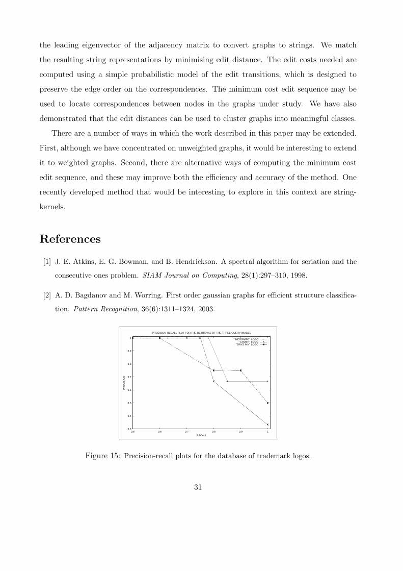
We have placed this study on a more quantitative basis by computing precision-recall

curves for the retrieval method. Figure 15 shows the precision-recall curves for the three

queries described above. It is the “Days-Inn” query that shows the fastest fall-off of precision

with recall. In the case of the remaining two queries, the fall-off does not take place until

the value of the recall is greater than 0.8.

6 Conclusions

The work reported in this paper provides a synthesis of ideas from spectral graph-theory

and structural pattern recognition. We use a graph spectral seriation method based on

30

the leading eigenvector of the adjacency matrix to convert graphs to strings. We match

the resulting string representations by minimising edit distance. The edit costs needed are

computed using a simple probabilistic model of the edit transitions, which is designed to

preserve the edge order on the correspondences. The minimum cost edit sequence may be

used to locate correspondences between nodes in the graphs under study. We have also

demonstrated that the edit distances can be used to cluster graphs into meaningful classes.

There are a number of ways in which the work described in this paper may be extended.

First, although we have concentrated on unweighted graphs, it would be interesting to extend

it to weighted graphs. Second, there are alternative ways of computing the minimum cost

edit sequence, and these may improve both the efficiency and accuracy of the method. One

recently developed method that would be interesting to explore in this context are string-

kernels.

References

[1] J. E. Atkins, E. G. Bowman, and B. Hendrickson. A spectral algorithm for seriation and the

consecutive ones problem. SIAM Journal on Computing, 28(1):297–310, 1998.

[2] A. D. Bagdanov and M. Worring. First order gaussian graphs for efficient structure classifica-

tion. Pattern Recognition, 36(6):1311–1324, 2003.

0.3

0.4

0.5

0.6

0.7

0.8

0.9

1

0.5 0.6 0.7 0.8 0.9 1

PR

EC

ISIO

N

RECALL

PRECISION-RECALL PLOT FOR THE RETRIEVAL OF THE THREE QUERY IMAGES

’’INCOGNITO’’ LOGO’’CRUSH’’ LOGO

’’DAYS INN’’ LOGO

Figure 15: Precision-recall plots for the database of trademark logos.

31

[3] H. Bunke. On a relation between graph edit distance and maximum common subgraph. Pattern

Recognition Letters, 18(8):689–694, 1997.

[4] H. Bunke, A. Munger, and X. Jiang. Combinatorial search vs. genetic algorithms: A case

study based on the generalized median graph problem. Pattern Recognition Letters, 20(11-

13):1271–1279, 1999.

[5] J. Canny. A computational approach to edge detection. IEEE Trans. on Pattern Analysis and

Machine Intelligence, 8(6):679–698, 1986.

[6] W. J. Christmas, J. Kittler, and M. Petrou. Structural matching in computer vision using

probabilistic relaxation. IEEE Transactions on Pattern Analysis and Machine Intelligence,

17(8):749–764, 1995.

[7] Fan R. K. Chung. Spectral Graph Theory. American Mathematical Society, 1997.

[8] E. W. Dijkstra. A note on two problems in connection with graphs. Numerische Math, 1:269–

271, 1959.

[9] C. Dorai and A.K. Jain. Shape spectrum-based view grouping and matching of 3d free-form

objects. EEE Trans. Pattern Analysis and Machine Intelligence, 19(10):1139–1145, 1997.

[10] M. A. Eshera and K. S. Fu. A graph distance measure for image analysis. IEEE Transactions

on Systems, Man and Cybernetics, 14:398–407, 1984.

[11] A. M. Finch, R. C. Wilson, and E. R. Hancock. An energy function and continuous edit

process for graph matching. Neural Computation, 10(7):1873–1894, 1998.

[12] S. Gold and A. Rangarajan. A graduated assignment algorithm for graph matching. PAMI,

18(4):377–388, April 1996.

[13] G. H. Golub and C. F. Van Loan. Matrix Computations. The Johns Hopkins Press, 1996.

[14] T. Hofmann and M. Buhmann. Pairwise data clustering by deterministic annealing. IEEE

Tansactions on Pattern Analysis and Machine Intelligence, 19(1):1–14, 1997.

[15] R. Horaud and H. Sossa. Polyhedral object recognition by indexing. Pattern Recognition,

28(12):1855–1870, 1995.

32

[16] B. Huet and E. R. Hancock. Relational object recognition from large structural libraries.

Pattern Recognition, 35(9):1895–1915, 2002.

[17] J. Keuchel, C. Schnorr, C. Schellewald, and D. Cremers. Binary partitioning, perceptual

grouping, and restoration with semidefinite programming. IEEE Trans. on Pattern Analysis

and Machine Intelligence, 25(11):1364–1379, 2003.

[18] J. J. Koenderink and A. J. van Doorn. Surface shape and curvature scales. Image and Vision

Computing, 10(8):557–565, 1992.

[19] V. I. Levenshtein. Binary codes capable of correcting deletions, insertions and reversals. Sov.

Phys. Dokl., 6:707–710, 1966.

[20] L. Lovasz. Random walks on graphs: a survey. Bolyai Society Mathematical Studies, 2(2):1–46,

1993.

[21] Bin Luo, A. D. J. Cross, and E. R. Hancock. Corner detection via topographic analysis of

vector-potential. Pattern Recognition Letters, 20(6):635 – 650, 1999.

[22] Bin Luo and E. R. Hancock. Structural graph matching using the EM algorithm and singular

value decomposition. IEEE Trans. on Pattern Analysis and Machine Intelligence, 23(10):1120–

1136, 2001.

[23] Bin Luo, R. C. Wilson, and E. R. Hancock. Spectral embedding of graphs. Pattern Recognition,

36:2213–2223, 2003.

[24] K. V. Mardia and P. E Jupp. Directional Statistics. John Wiley & Sons, 2000.

[25] B. Mohar. Some applications of laplace eigenvalues of graphs. In G. Hahn and G. Sabidussi,

editors, Graph Symmetry: Algebraic Methods and Applications, NATO ASI Series C, pages

227–275, 1997.

[26] R. Myers, R. C. Wilson, and E. R. Hancock. Bayesian graph edit distance. PAMI, 22(6):628–

635, June 2000.

[27] Yin Peng-Yeng. Algorithms for straight line fitting using k-means. Pattern Recognition Letters,

19:31–41, 1998.

33

[28] A. Robles-Kelly and E. R. Hancock. A probabilistic spectral framework for spectral clustering

and grouping. Pattern Recognition, 37(7):1387–1405, 2004.

[29] A. Robles-Kelly and E. R. Hancock. String edit distance, random walks and graph matching.

Int. Journal of Pattern Recognition and Artificial Intelligence, 18(3):315–327, 2004.

[30] A. Robles-Kelly, S. Sarkar, and E. R. Hancock. A fast leading eigenvector approximation

for segmentation and grouping. In International Conference on Pattern Recognition, pages

I:639–642, 2002.

[31] A. Sanfeliu and K. S. Fu. A distance measure between attributed relational graphs for pattern

recognition. IEEE Transactions on Systems, Man and Cybernetics, 13:353–362, 1983.

[32] G. Scott and H. Longuet-Higgins. An algorithm for associating the features of two images. In

Proceedings of the Royal Society of London, number 244 in B, pages 21–26, 1991.

[33] B. Selman, H. A. Kautz, and B. Cohen. Noise strategies for improving local search. In Proc.

of the Twelfth National Conference on Artificial Intelligence, pages 337–343, 1994.

[34] L. G. Shapiro and R. M. Haralick. Relational models for scene analysis. IEEE Transactions

on Pattern Analysis and Machine Intelligence, 4:595–602, 1982.

[35] L. S. Shapiro and J. M. Brady. A modal approach to feature-based correspondence. In British

Machine Vision Conference, pages 78–85, 1991.

[36] A. Shokoufandeh, S. J. Dickinson, K. Siddiqi, and S. W. Zucker. Indexing using a spectral

encoding of topological structure. In Proceedings of the Computer Vision and Pattern Recog-

nition, pages 491–497, 1998.

[37] O. Steinmann, A. Strohmaier, and T. Stutzle. Tabu search vs. random walk. In Advances in

Artificial Intelligence (KI-97), pages 337–348, 1997.

[38] G. W. Stewart and Ji-Guang Sun. Matrix Perturbation Theory. Academic Press, 1990.

[39] M. Tuceryan and T. Chorzempa. Relative sensitivity of a family of closest-point graphs in

computer vision applications. Pattern Recognition, 24(5):361–373, 1991.

[40] S. Umeyama. An eigen decomposition approach to weighted graph matching problems. PAMI,

10(5):695–703, September 1988.

34

[41] R. S. Varga. Matrix Iterative Analysis. Springer, second edition, 2000.

[42] R. A. Wagner and M. J. Fisher. The string-to-string correction problem. Journal of the ACM,

21(1):168–173, 1974.

[43] R. C. Wilson and E. R. Hancock. A bayesian compatibility model for graph matching. Pattern

Recognition Letters, 17:263–276, 1996.

[44] R.C. Wilson and E. R. Hancock. Structural matching by discrete relaxation. IEEE Transac-

tions on Pattern Analysis and Machine Intelligence, 19(6):634–648, June 1997.

[45] P. L. Worthington and E. R. Hancock. New constraints on data-closeness and needle map

consistency for shape-from-shading. IEEE Transactions on Pattern Analysis and Machine

Intelligence, 21(12):1250–1267, 1999.

35