graph grammars and operations on graphs
TRANSCRIPT
Graph Grammars and
Operations on Graphs
Jan Joris Vereijken
May 19, 1993
Department of Computer Science
Leiden University
The Netherlands

ii
Master’s Thesis, Leiden University, The Netherlands.
Title : Graph Grammars and Operations on Graphs
Author : Jan Joris Vereijken
Supervisor : Dr. Joost Engelfriet
Completion date : May 19, 1993
Copyright c©1993 • Jan Joris Vereijken • Leiden Typeset by AMS-LaTEX.

iii
Problems worthy
of attack
prove their worth
by hitting back.


Contents
1 Introduction 1
1.1 Graph grammars . . . . . . . . . . . . . . . . . . . . . . . . . . . . . . . . 1
1.2 The structure of this thesis . . . . . . . . . . . . . . . . . . . . . . . . . . . 2
1.3 Closing remarks . . . . . . . . . . . . . . . . . . . . . . . . . . . . . . . . . 4
2 Definitions 5
2.1 Terminology . . . . . . . . . . . . . . . . . . . . . . . . . . . . . . . . . . . 5
2.2 Typing . . . . . . . . . . . . . . . . . . . . . . . . . . . . . . . . . . . . . . 8
2.3 Typed alphabets . . . . . . . . . . . . . . . . . . . . . . . . . . . . . . . . 9
2.4 Typed languages . . . . . . . . . . . . . . . . . . . . . . . . . . . . . . . . 10
2.5 Typed grammars . . . . . . . . . . . . . . . . . . . . . . . . . . . . . . . . 11
2.6 Typed languages versus typed grammars . . . . . . . . . . . . . . . . . . . 12
3 I/O-hypergraphs 17
3.1 Definition . . . . . . . . . . . . . . . . . . . . . . . . . . . . . . . . . . . . 17
3.2 Terminology . . . . . . . . . . . . . . . . . . . . . . . . . . . . . . . . . . . 18
3.3 Depiction of hypergraphs . . . . . . . . . . . . . . . . . . . . . . . . . . . . 19
3.4 Ordinary graphs . . . . . . . . . . . . . . . . . . . . . . . . . . . . . . . . . 20
3.5 String graphs . . . . . . . . . . . . . . . . . . . . . . . . . . . . . . . . . . 20
3.6 External versus internal nodes . . . . . . . . . . . . . . . . . . . . . . . . . 22
3.7 Hypergraph languages . . . . . . . . . . . . . . . . . . . . . . . . . . . . . 22
3.8 Union of hypergraph languages . . . . . . . . . . . . . . . . . . . . . . . . 23
4 Composition 25
4.1 Sequential composition . . . . . . . . . . . . . . . . . . . . . . . . . . . . . 25
4.2 Sequential composition versus degree and loops . . . . . . . . . . . . . . . 27
4.3 Parallel composition . . . . . . . . . . . . . . . . . . . . . . . . . . . . . . 28
4.4 Sequential versus parallel composition . . . . . . . . . . . . . . . . . . . . . 29
v

vi Contents
4.5 Expressions used as a function . . . . . . . . . . . . . . . . . . . . . . . . . 31
5 Decomposition 33
5.1 Definition . . . . . . . . . . . . . . . . . . . . . . . . . . . . . . . . . . . . 33
5.2 HGR·
−→ LA . . . . . . . . . . . . . . . . . . . . . . . . . . . . . . . . . . 34
5.3 LA·
−→ LB . . . . . . . . . . . . . . . . . . . . . . . . . . . . . . . . . . . . 35
5.4 LB·
−→ LC2 ∪ LC3 . . . . . . . . . . . . . . . . . . . . . . . . . . . . . . . . 36
5.5 LC3
·,+−→ LC1 ∪ LC2 . . . . . . . . . . . . . . . . . . . . . . . . . . . . . . . 37
5.6 LC2
·,+−→ LC4 ∪ LC5 . . . . . . . . . . . . . . . . . . . . . . . . . . . . . . . 37
5.7 LC4
·,+−→ LC6 . . . . . . . . . . . . . . . . . . . . . . . . . . . . . . . . . . . 40
5.8 LC5
·,+−→ LC6 . . . . . . . . . . . . . . . . . . . . . . . . . . . . . . . . . . . 41
5.9 LB·,+−→ LC . . . . . . . . . . . . . . . . . . . . . . . . . . . . . . . . . . . 41
5.10 Conclusions . . . . . . . . . . . . . . . . . . . . . . . . . . . . . . . . . . . 41
6 Folds and flips 43
6.1 Definition . . . . . . . . . . . . . . . . . . . . . . . . . . . . . . . . . . . . 43
6.2 Basic properties . . . . . . . . . . . . . . . . . . . . . . . . . . . . . . . . . 44
6.3 Derived properties . . . . . . . . . . . . . . . . . . . . . . . . . . . . . . . 45
7 Interpretation 47
7.1 Definition of an interpreter . . . . . . . . . . . . . . . . . . . . . . . . . . . 47
7.2 Definition of Int . . . . . . . . . . . . . . . . . . . . . . . . . . . . . . . . . 48
7.3 Examples of interpretation . . . . . . . . . . . . . . . . . . . . . . . . . . . 49
7.4 Edge Normal Form . . . . . . . . . . . . . . . . . . . . . . . . . . . . . . . 51
7.5 Existence of isomorphic copies . . . . . . . . . . . . . . . . . . . . . . . . . 52
7.6 Bounded degree implies bounded cutwidth . . . . . . . . . . . . . . . . . . 53
8 Power of interpretation 57
8.1 Int(RLIN) = Int(LIN) . . . . . . . . . . . . . . . . . . . . . . . . . . . . . 57
8.2 Int(RLIN) = Int(DB) . . . . . . . . . . . . . . . . . . . . . . . . . . . . . . 64
8.3 Int(STR(Int(K))) = Int(K) . . . . . . . . . . . . . . . . . . . . . . . . . . . 72
8.4 About STR(Int(RLIN)) . . . . . . . . . . . . . . . . . . . . . . . . . . . . 78
8.5 The power of interpretation theorems . . . . . . . . . . . . . . . . . . . . . 79
8.6 Conclusions . . . . . . . . . . . . . . . . . . . . . . . . . . . . . . . . . . . 80
9 Closure properties of Int(K) 83
9.1 Closure under sequential composition . . . . . . . . . . . . . . . . . . . . . 83
9.2 Closure under union . . . . . . . . . . . . . . . . . . . . . . . . . . . . . . 84
Contents vii
9.3 Closure under Kleene closure . . . . . . . . . . . . . . . . . . . . . . . . . . 84
9.4 Closure under +Un and Un+ . . . . . . . . . . . . . . . . . . . . . . . 85
9.5 Closure under parallel composition . . . . . . . . . . . . . . . . . . . . . . 86
9.6 Closure under fold and backfold . . . . . . . . . . . . . . . . . . . . . . . . 86
9.7 Closure under flip . . . . . . . . . . . . . . . . . . . . . . . . . . . . . . . . 86
9.8 Closure under split . . . . . . . . . . . . . . . . . . . . . . . . . . . . . . . 88
9.9 Closure under edge relabeling . . . . . . . . . . . . . . . . . . . . . . . . . 88
9.10 Conclusions . . . . . . . . . . . . . . . . . . . . . . . . . . . . . . . . . . . 88
10 Another characterization 91
10.1 Using HGR . . . . . . . . . . . . . . . . . . . . . . . . . . . . . . . . . . . 91
10.2 Using the sequential pseudo base set . . . . . . . . . . . . . . . . . . . . . 92
10.3 Using the full base set . . . . . . . . . . . . . . . . . . . . . . . . . . . . . 93
10.4 Conclusions . . . . . . . . . . . . . . . . . . . . . . . . . . . . . . . . . . . 93
11 Other literature 95
11.1 Introduction . . . . . . . . . . . . . . . . . . . . . . . . . . . . . . . . . . . 95
11.2 Engelfriet and Heyker . . . . . . . . . . . . . . . . . . . . . . . . . . . . . . 96
11.3 Context-Free Hypergraph Grammars . . . . . . . . . . . . . . . . . . . . . 97
11.4 split(Γ(LIN-CFHG)) = Int(RLIN) . . . . . . . . . . . . . . . . . . . . . . . 98
11.5 Int(RLIN) Int(CF) . . . . . . . . . . . . . . . . . . . . . . . . . . . . . . 101
11.6 Int(CF) split(Γ(CFHG)) . . . . . . . . . . . . . . . . . . . . . . . . . . . 102
11.7 Bauderon and Courcelle . . . . . . . . . . . . . . . . . . . . . . . . . . . . 104
11.8 Habel and Kreowski . . . . . . . . . . . . . . . . . . . . . . . . . . . . . . 106
11.9 Further reading . . . . . . . . . . . . . . . . . . . . . . . . . . . . . . . . . 107
12 Summary 109
13 Acknowledgments 111
A Naming conventions 113
B Proofs 117
B.1 Proofs concerning Section 6.3 . . . . . . . . . . . . . . . . . . . . . . . . . 117
B.2 Proofs concerning Section 8.2 . . . . . . . . . . . . . . . . . . . . . . . . . 120
Bibliography 127
Index 129


For those who like this sort of thing,
this is the sort of thing they like.
— Abraham Lincoln 1Introduction
1.1 Graph grammars
Just like sets of strings (string languages) can be characterized by string grammars, sets of
graphs (graph languages) can be characterized by graph grammars. Over the past decade,
a lot of research has been done into this subject. The approach mainly taken was either
to rewrite edges, or to rewrite nodes.
However, a completely different approach to define graph languages is also imaginable:
one defines a number of operations on graphs (including constants), and considers a string
language of expressions over these operations. The graphs obtained by evaluating these
expressions then form a graph language.
In this thesis we describe and investigate a simple formalism of the latter kind. We
define only one nonconstant operation on graphs: sequential composition.
When we now take a string language over some alphabet, and a function from that
alphabet to a set of graphs, we can do the following. For each string in the language, take
the graphs one obtains by applying the function to all the symbols that form that string.
Now take the sequential composition of all those graphs, in the order as indicated by the
order of the symbols that form the string. This yields a graph. So, for every string in
the language, we obtain a graph. Together they form a graph language. We have called
this formalism interpretation: we take a string language and a function, and interpret
the strings in that language as graphs, in the way indicated by that function (called the
interpreter). Note that the symbols in the alphabet may be viewed as graph constants,
1
2 Introduction
that can be arbitrarily interpreted as graphs, by the interpreter. Strings may be viewed
as expressions over these constants and sequential composition. Thus, concatenation of
strings is interpreted as sequential composition of graphs.
This formalism to associate graph languages with string languages has the following
obvious advantage above a graph grammar formalism. From formal language theory, a lot
of different classes (for example, the Chomsky hierarchy) of string languages are known.
By means of interpretation, we can immediately derive classes of graph languages from
these classes of string languages. For example, from the class of all regular languages, we
instantly derive the class of all graph languages obtainable by interpretation of regular
languages. In this way, for every known class of string languages, we now also have a
corresponding class of graph languages.
In the chapters to follow, we will investigate the relations between several classes ob-
tained by interpretation in this way. We will look at their properties, and how our formalism
relates to other formalisms (mainly graph grammars) that were proposed to define graph
languages. That brings us to the title of this thesis: “Graph Grammars and Operations
on Graphs”. In our view, a string grammar/interpreter pair is just a “graph grammar in
disguise”. This will be justified by the results we will find; they are very much alike the
results obtained by using a “real” graph grammar.
1.2 The structure of this thesis
The structure of this thesis is the following. In Chapter 2, we lay out the mathematical
framework needed to express ourselves. In particular, we will introduce the concept of typ-
ing: every symbol, string, string language, graph, or whatever, has two integers associated
with it, its input type, and its output type.
As we will want to interpret concatenation as sequential composition, we will need a
special kind of graphs, namely i/o-hypergraphs (Chapter 3). These have distinguished input
nodes and output nodes, so we have an easy way to define how the sequential composition
acts on them: roughly speaking, sequential composition connects two graphs to one another
by “hooking” the first’s output nodes to the second’s input nodes, just like railroad cars
are hooked together to form a train. By the typing, we indicate the number of nodes that
need to be hooked. If we now make sure that the types of two neighboring symbols within
a string match, and that the interpretation function preserves the type of the symbols, we
can guarantee that in the process of interpreting we will only apply sequential composition
to graphs that “fit”. This is, in short, the reason we need all our objects to be typed:
to ensure that all our operations are applied in a way that makes sense, i.e., the objects
operated on must fit.

The structure of this thesis 3
Then, in Chapter 4, we formally define the sequential composition operation, and its less
important counterpart, parallel composition. Using these operations, we can take “small”
graphs, and use them to build larger ones. As noted, sequential composition is like hooking
railroad cars together, with graphs. Continuing this metaphor, parallel composition is like
stacking railroad cars on top of one another (for example, in order to build a double-deck
automobile carrier).
Just like the composition operations build larger graphs form small ones, we can also
do the opposite: take a large graph to pieces, namely small graphs. In Chapter 5, we
investigate this process, which is called decomposition. We will try to find the “smallest”
set of “small” graphs from which all other ones can be built. Or in other words, we search
for the “basic building blocks” of graphs (the answer, more or less, is: edges).
In Chapter 6 we introduce four auxiliary operations on graphs. These operations do not
operate on the internal structure of graphs, but only on the “superficial” structure of which
distinguished nodes are input nodes, and which ones are output nodes. Some properties of
these operations are investigated. They will “only” be needed to conveniently express the
technical details of some proofs, but nonetheless they have a beauty of their own.
After that, in Chapter 7, we are finally ready to introduce the formalism of interpreta-
tion, and will devote three chapters to the investigation of its power and properties. First
of all, we will prove some theorems about classes of graph languages obtained by interpre-
tation, one of them concerning a normal form for interpretation. Most importantly, these
theorems will gain us an insight in the structure of these kinds of classes.
Then, in Chapter 8, we look at the classes of regular, linear, and derivation-bounded
languages under interpretation. As it turns out, all three give rise to the same class, which
we propose as the “class of regular graph languages”. Furthermore, we indicate how large
a class can get so that under interpretation it is still the same as the class of all regular
graph languages. This culminates in the two “power of interpretation” theorems, which
give strong indications on the power of interpretation.
In Chapter 9 we look at some closure properties of a general class of graph languages
obtained by interpretation. The conditions for closure will be given in terms of closure
properties of the underlying class of string languages on which the interpretation acted.
Following that, there are two chapters where we make comparisons with other for-
malisms. In Chapter 10 we give a “smallest class closed under . . . ” characterization of the
class of all regular graph languages, and in Chapter 11 we look at the relations between
the formalism of interpretation and some other formalisms that have been proposed in the
literature. Luckily, our idea of “the class of regular graph languages” corresponds very well
with some classes proposed by other researchers.
There are two appendices. In Appendix A we account for the naming conventions (e.g.,
4 Introduction
n is always an integer, w is always a string of symbols) we have used throughout this thesis.
By strictly adhering to these conventions, we hope to have made our constructions easier
to read. Appendix B contains some proofs that we did not want in give in full in the main
text.
Finally, there is a Bibliography, which contains information about the literature we
refer to, and an extensive Index.
1.3 Closing remarks
This Master’s thesis was written in the final fulfillment of the requirements for a Master’s
degree in Theoretical Computer Science at the Rijksuniversiteit te Leiden, The Netherlands,
under the supervision of Dr. Joost Engelfriet.
For those curious, the motto on page iii appeared as a fortune cookie on my computer
terminal one winter night at 4:30 AM, when after a whole night of TEX’ing and fiddling
with the definition of interpretation, I found out that I had “fixed” the definition, but
broken all my proofs, seemingly beyond repair. Disillusioned I logged out of our vax/vms
system, only to end up with a screen that said, in large, friendly, VT100 letters:
Problems worthy of attack prove
their worth by hitting back.
It seemed very appropriate.

We will restrict ourselves to natural numbers
only, as there are quite enough of these.
— Edsger Wybe Dijkstra 2Definitions
In this chapter the definitions and notations are laid out of the mathematical framework
we will need. Some of them are very common, and in wide use, and some are quite novel.
In particular, we introduce typed variants of the concepts of a grammar and a language,
as noted in the introduction.
2.1 Terminology
We assume the reader to be familiar with elementary set theory (see, e.g., [Kam50], [BS87,
§5], or [Her75, §1.1]), and elementary formal language theory (see, e.g., [HU79] or [CL89]).
Some basic knowledge about graphs is also useful (see, e.g., [BS87, §11] or [Joh84, §3]).
Numbers: N denotes the set 0, 1, 2, . . . of all nonnegative natural numbers. The in-
terval 1, . . . , n is denoted by [n], and the interval m, . . . , n by [m, n]. For a finite set
V N, by max(V ) we denote the largest element of V , and by min(V ) the smallest
element.
Sets: Set inclusion is denoted by ⊆, proper set inclusion by , set union by ∪, set
intersection by ∩. Set difference is denoted by \ or −. The symbols ⊇ and ! denote the
inverses of ⊆ and . The empty set is denoted by ∅, set membership by ∈, or inversely,
3. For a set V , P(V ) denotes the power set of V ; P(V ) = W | W ⊆ V . The cardinality
5

6 Definitions
of a set V is denoted1 by |V |. The cartesian product of two sets V and W is denoted by
V × W , and the n times repeated cartesian product of a set V with itself by V n.
Sequences: A sequence over a set V is denoted (v1, . . . , vn), the empty sequence () by λ,
and V ∗ denotes the set of all sequences. The length of a sequence α ∈ V ∗ is denoted by |α|.
A sequence of length n will also be called an n-sequence.
Logic: By TRUE and FALSE we denote the boolean constants for true and false. Logical
or is denoted by ∨, and logical and by ∧. The symbol =⇒ denotes logical implication,
and ⇐⇒ logical equivalence (if and only if). We follow the convention to write “iff”
as a shorthand for “if and only if”. The symbol ∀ denotes universal quantification (“for
all”) and ∃ denotes existential quantification (“there exists”). These quantors are always
subscripted by the declarations of the variables that are local to the quantification, e.g.,
∀a,b,c,n∈N+ (n ≥ 3 =⇒ an + bn 6= cn). Name clash ambiguities between local and global
variables are not allowed.
Relations: The symbol ≡ always denotes an equivalence relation. For a set V and an
equivalence relation ≡ on V , the equivalence class of v ∈ V with respect to ≡ is denoted
by [v]≡, and the set of all equivalence classes by V/≡. An equivalence relation ≡ on some
set V may be thought of as a set, namely the set (v, v′) ∈ V × V | v ≡ v′ of all pairs
from V that are equivalent.
We extend the notation to sequences and functions in the following way. For a sequence
(v1, . . . , vn) over a set V , and ≡ an equivalence relation on V , by [(v1, . . . , vn)]≡ we denote
the sequence ([v1]≡, . . . , [vn]≡). For a function f : V1 → V2 and an equivalence relation ≡
on V , the function f≡ is defined as f≡(v) = [f(v)]≡, for all v ∈ V1. By the symbol ≈ we
denote the informal concept of “approximate” equality. Formally, ≈ means nothing at all !
Functions: For two functions f : V1 → V2 and g : V2 → V3 the composition is written as
g f , and for all v ∈ V1, (g f)(v) = g(f(v)). The restriction of a function f : V → W
to a subset V ′ of V is denoted f V ′. A function f : V → W whose domain V contains
exactly one element may be denoted a 7→ f(a), where a is that one element. For a bijective
function (also called bijection) f : V1 → V2, its inverse is denoted f−1 : V2 → V1.
Alphabets: An alphabet (also called ordinary alphabet) is a nonempty finite set of sym-
bols. A ranked alphabet is an alphabet that has a rank from N associated with every
1Warning : the symbol # is only used in identifier names, not to denote set cardinality.

Terminology 7
symbol. For an alphabet Σ and a symbol a ∈ Σ, this rank is denoted as rankΣ(a). To
express its rank, a symbol a with rank n may be denoted (a, n).
Strings: A string2 over an alphabet Σ is a sequence w ∈ Σ∗, a substring v ∈ Σ∗ of a
string w ∈ Σ∗ is a string such that there exists strings u, z ∈ Σ∗ such that uvz = w. If
u = λ the string v is called a prefix of w, and if furthermore v and z are both nonempty
it is called a proper prefix. Conversely, when z = λ, the string v is called a postfix, and a
proper postfix if also u and v are nonempty. By the symbol · we denote the concatenation
of strings. For a string w = a1 . . . an its reverse an . . . a1 is denoted by wR. This operation
is called reversal. A language over an alphabet Σ is a set L ⊆ Σ∗, in other words, a set
of strings over Σ. If we say that L is strictly over Σ, we mean that all symbols are really
used, i.e., for all a ∈ Σ there exists a string w ∈ L such that a is a substring of w.
Grammars: A context-free grammar is denoted G = (N, T, P, S), where N is the non-
terminal alphabet, T is the terminal alphabet (disjoint with N), P is the set of productions
(of the form A → α with A ∈ N , and α ∈ (N ∪ T )∗), and S ∈ N is the initial symbol. A
derivation of an α ∈ (N ∪ T )∗ by a nonterminal A ∈ N will be denoted A ⇒∗ α. When
we want to explicitly mention the length k of the derivation, we write A ⇒k α. We may
prefix any of these syntactic constructs by the name G of the grammar in order to stress
to which grammar it belongs. E.g.: G : A ⇒∗ α, meaning A derives α in G. The set of all
context-free grammars is denoted by G(CF). For a context-free grammar G the language
it defines is denoted L(G).
Classes of languages: The class of all context-free languages, L(G) | G ∈ G(CF) is
denoted by L(CF). The following well-known classes of context-free languages are used in
this thesis: L(RLIN), the class of all right-linear languages, L(LIN), the class of all linear
languages and L(DB), the class of all derivation-bounded languages. Where there can be
no confusion, we may omit the L’s.
A language L is said to be right-linear iff it can be generated by a context-free grammar
G that satisfies the restriction that for every p ∈ P , p is of the form A → wB, or A → w,
where A, B ∈ N and w ∈ T ∗. Such a grammar G is also called right-linear. The class of all
right-linear languages is also often called the class of all regular languages, and therefore,
sometimes denoted as REG.
A language L is linear iff it can be generated by a context-free grammar G that satisfies
the restriction that for every p ∈ P , p is of the form A → vBw, or A → v, where A, B ∈ N
and v, w ∈ T ∗. Such a grammar G is also called linear.
2Traditionally, strings are also often called words.
8 Definitions
A language L is derivation-bounded iff it can be generated by a context-free grammar G
such that for some m ∈ N, for every w ∈ L there is a derivation S ⇒ α1 ⇒ · · · ⇒ αn ⇒ w,
where αi ∈ (N ∪ T )∗, in G such that there is no αi that contains more than m occurrences
of symbols from N . This bound m is called the derivation bound. Such a grammar G is
also called derivation-bounded.
The relation between the above mentioned classes of languages is RLIN LIN DB
CF (note that all inclusions are proper).
Formally, if X is a property of a grammar, then G(X) is the class of all grammars
that have that property, and L(X) = L(G) | G ∈ G(X) is the class of all languages
generated by those grammars. So, strictly speaking, RLIN (for example) is a property of
grammars (namely, right-linearity), G(RLIN) is a class of grammars, and L(RLIN) is a
class of languages. As noted, we will informally often omit the L, and use X to denote
L(X).
2.2 Typing
As noted in the introduction, we want our objects to be “typed”. That is, with almost
every object, be it a symbol, an alphabet, a language, or whatever, we want to associate a
type, denoted (m → n) (where m, n ∈ N).
The general idea behind this is twofold. Firstly, for some our functions we will want
to require type preservingness, i.e., the function must always return an object of the same
type as the object it took as argument. Secondly, we will want to specify type conditions,
i.e., some binary operations will only be defined under certain conditions on the types of
the two arguments. In this way, we can always assure that the results of our computations
are defined and meaningful.
Compare this to what happens in strongly typed programming languages. Take for
example pascal. There all variables have to be declared, and must be used in accordance
with their declaration. So when, e.g., we declare var n:integer; x:real; the assignment
x := sqrt(n); makes sense, but n := sqrt(x); will result in a compile-time error. Or
compare it to what happens in physics, where we have the concept of unit. We are only
allowed to operate on quantities in a way that makes sense with respect to their respective
units. So, one kilogram plus two kilograms makes three, but two meters plus four seconds
is always nonsense. Just as obeying the declarations in pascal program, and the units in
a physical computation, is a sine qua non for the results to make sense, we will have to
obey certain rules of typing too.
The reason that we want to give each object an input type and an output type, is that
our graphs (to be defined later) will have two distinguished types of nodes: input nodes,

Typed alphabets 9
and output nodes. Intuitively, an object of type (m → n) stands as a placeholder for a
graph with m input nodes and n output nodes.
In the three sections to follow, we will define typed variants of the concepts of an
alphabet, a language and a grammar.
2.3 Typed alphabets
A typed alphabet is an alphabet that has two ranks from N associated with every symbol.
For an alphabet Σ and a symbol a ∈ Σ, these two ranks are denoted as #inΣ(a) (the input
type) and #outΣ(a) (the output type). We may drop the subscribed Σ where there can be
no confusion. A symbol a ∈ Σ with input type m and output type n may also be denoted
(a, m → n). It is said to be of type (m → n). If we want to stress the fact that a symbol
belongs to a typed alphabet, we may call it a typed symbol. Consequently, a symbol from
an ordinary alphabet may be called an ordinary symbol. Mutatis mutandis, we define a
typed set to be a set that has two ranks from N associated with every element, and refer
to a nontyped set as an ordinary set.
A typed alphabet Σ1 and an ordinary alphabet Σ2 such that both contain exactly the
same symbols are considered equal (denoted Σ1 = Σ2), albeit there are two functions
that are defined on the first that are undefined on the second (also see the “philosophical
sidenote” at the end of Section 2.4).
Let Σ be a typed alphabet. For two symbols a1, a2 ∈ Σ, the concatenation w = a1 ·a2 is
only defined when #out(a1) = #in(a2). The type of the resulting string w is (#in(a1) →
#out(a2)). Kleene closure on Σ is defined as follows:
Σ+ = a1 . . . an | n ≥ 1,#outΣ(ai) = #inΣ(ai+1) for 1 ≤ i < n, a1, . . . , an ∈ Σ ,
Σ∗ = (λ, n → n) | n ∈ N ∪ Σ+.
Here (λ, n → n) denotes the empty string of type (n → n) (note that there is no such
thing as a (λ, m → n) where m 6= n). For a nonempty string w ∈ Σ∗, α = a1 . . . an the
input type of w, denoted #inΣ(w), is #inΣ(a1). The output type, denoted #outΣ(w), is
#outΣ(an). A string w ∈ Σ∗ of type (m → n) can be denoted (w, m → n). Note that Σ∗
is a typed set.
A string w = a1 . . . an over a typed alphabet Σ is called correctly internally typed if
#outΣ(ai) = #inΣ(ai+1) for all 1 ≤ i < n. Note that, by the above definition of Kleene
closure on a typed set, Σ∗ consists of exactly all correctly internally typed strings over Σ.
Concatenation of two strings v, w ∈ Σ∗ is only defined when the output type of the first
10 Definitions
matches the input type of the second. So for (v, m → n) and w, n → k) we define:
(v, m → n) · (w, n → k) = (vw, m → k).
Note that for a string v ∈ Σ∗ all substrings of w are also in Σ∗. By definition of a substring,
the empty string (λ, n → n) is a substring of v iff there is a symbol a ∈ Σ in v such that
#inΣ(a) = n or #outΣ(a) = n.
As with symbols, we will use the terms ordinary string and typed string to discriminate
between the two.
2.4 Typed languages
A typed language L is a set of correctly internally typed strings over some typed alphabet
Σ, such that all strings have the same type:
∀w1,w2∈L (#in(w1) = #in(w2) and #out(w1) = #out(w2)) .
A typed language L in which all strings are of type (m → n) can be denoted (L, m → n)
when clarity demands it. We say that L is of type (m → n). If necessary, the input and
output type can be denoted as follows: #in(L) = m and #out(L) = n. In the case of the
empty language of type (m → n), we need to write (∅, m → n) to make its type explicit.
If m = n, L is called of uniform type. Note that a typed language that contains the empty
string λ must necessarily be of uniform type: a typed λ always has the same input and
output type, say (λ, k → k), for some k ∈ N, and all strings in L have the same type, so
L has type (k → k).
Concatenation, union, and Kleene closure are defined on typed languages over the same
alphabet Σ in the following way (let (L, m → n), (L1, m1 → n1) and (L2, m2 → n2) be
typed languages).
• L1 · L2 = w1 · w2 | w1 ∈ L1 and w2 ∈ L2 , in the case that n1 = m2, and undefined
otherwise. Note that L1 · L2 is of type (m1 → n2),
• L1 ∪ L2 = w | w ∈ L1 or w ∈ L2 , in the case that m1 = m2 and n1 = n2, and
undefined otherwise. Note that L1 ∪ L2 is of type (m1 → n1),
• L∗ =⋃∞
k=0 Lk, in the case that m = n, and undefined otherwise. Here Lk denotes L, k
times concatenated to itself. L0 denotes the appropriate unity element, (λ, m → m)
in this case. Note that L∗ is of type (m → m).
Typed grammars 11
Finally, when we want to stress the fact that a string language is not typed, we will refer
to it as an ordinary string language. For a typed string language L, the ordinary string
language L′ such that L and L′ contain exactly the same strings (albeit those in L are
typed, and those in L′ are not) is called the underlying language of L′.
For a class K of ordinary string languages, we denote by Lτ (K) the class of all typed
languages whose underlying languages are in L(K). Note that since we use X to denote
L(X), Lτ (X) denotes Lτ (L(X)).
As a “philosophical” sidenote: normally we would consider two languages equal iff they
contain exactly the same strings. In order to remain faithful to this intuitive concept, we
will allow a typed language L1 and a nontyped language L2 to be equal to each other, albeit
that nonetheless there is a difference: the strings in L1 have a type associated with them,
those in L2 do not. This (non)typing, however, is not considered to be all that important
for the essence of the language, it is merely something that is added on for convenience.
We will write: L1 = L2.
If all this sounds counter-intuitive, notice that something similar is being done in or-
dinary formal language theory, where two languages over different alphabets can be the
same, provided only a common subset of symbols from both alphabets is actually used in
the two languages.
In other words: not where the symbol came from (the one alphabet or the other)
matters, but what the symbol is.
Note that from this point of view L(CF) = Lτ (CF)! (Proof: assign type (0 → 0)
to all symbols.) So when we write L ∈ Lτ (CF) formally speaking we could just as well
have dropped the τ . However, in what follows we will implicitly assume that the τ in
L ∈ Lτ (CF) means that we have a fixed typing in mind for that L.
Unfortunately, this also prohibits us from writing L1 = L2, if, for two typed languages
L1, L2, we want to express that they are equal and also have the same typing defined on
them (or = would not be an equivalence relation anymore, something we certainly do not
want to happen). Therefore, we will write L1 =τ L2 instead, if we want to express that
L1 = L2 and L1, L2 ⊆ Σ∗ for some typed alphabet Σ, i.e., L1 and L2 are equal even with
the typing. Note that =τ indeed is an equivalence relation.
2.5 Typed grammars
A context-free grammar G = (N, T, P, S) where N and T are typed alphabets is called
typed, if for every production p : A → α, A ∈ N , α ∈ (N ∪ T )∗, A and α are of the
same type. Be aware that the Kleene closure is over a typed alphabet, so α is a correctly
internally typed string with respect to N ∪ T . Let G′ = (N ′, T ′, P ′, S ′) be the underlying

12 Definitions
grammar of G, i.e., N ′ = N , T ′ = T (albeit there is no typing defined on N ′ and T ′),
P ′ = P , and S ′ = S. We now define L(G), the typed language generated by the typed
grammar G:
L(G) =
L(G′), typed according to T if L(G′) 6= ∅,
(∅,#inN(S) → #outN(S)) if L(G′) = ∅
Warning : note that this definition only makes sense if L(G′) is a typed language with
respect to T . That this is indeed the case, will be proved in the next section, where we
will also prove that L(G) is always of the same type as S.
When we want to stress the fact that a grammar is not typed, we will refer to it as an
ordinary grammar.
We extend the notation G(X), all grammars with a certain property, (for example,
X = CF), to Gτ (X), all typed grammars whose underlying grammar is in G(X).
2.6 Typed languages versus typed grammars
Context-free typed languages and typed grammars are equivalent in the sense that every
typed grammar generates a context-free typed language, and that every context-free typed
language is generated by some context-free typed grammar. Formally:
∀G∈Gτ (CF) L(G) ∈ Lτ (CF),
and
∀L∈Lτ (CF) ∃G∈Gτ (CF) L =τ L(G).
(2.1)
Part 1:
Firstly, we will prove that for every typed context-free grammar G, we have L(G) ∈
Lτ (CF)3. Let G = (N, T, P, S) ∈ Gτ (CF), and G′ = (N ′, T ′, P ′, S ′) the underlying gram-
mar of G. Now for every production p : A → α, A ∈ N , α ∈ (N ∪ T )∗, we have, by
definition, #inN(A) = #in(N∪T )(α), and #outN(A) = #out(N∪T )(α). To start with, we
will prove that for every derivation:
G′ : S ′ ⇒∗ α,
where α ∈ (N ′ ∪ T ′)∗, we have that:
• α is correctly internally typed with respect to N ∪ T , and,
3Formally speaking, this is trivially true (by definition)! Recall however the above warning that we still
need to verify that the definition is correct. This verification is what the now following proof is about.
Typed languages versus typed grammars 13
• with respect to N ∪ T , α is of the same type as S ′.
We proceed by induction on the length of the derivation. Induction basis: length is 0.
There is only one derivation of length 0: S ′ ⇒0 S ′, for which both conditions trivially hold.
Induction step: length is k + 1. We assume that our claim holds for length k. Consider a
derivation of length k + 1, which has the form:
S ′ ⇒k αp⇒ β.
To prove: β is correctly internally typed, and has the same type as S ′. Let the production
applied in the last step be p : A′ → γ. Then α must have the form α′A′α′′, and consequently
β the form α′γα′′. As α is correctly typed internally, by the induction hypothesis, so are
α′ and α′′. And, as A′ has the same type as γ, and γ is correctly typed internally (both
by the definition of p), necessarily β is correctly typed internally also. Furthermore, as
obviously β has the same type as α, and, by the induction hypothesis, α has the same type
as S ′, it is clear that β has the same type as S ′. End of induction proof.
Now for any w ∈ T ′∗ in L(G′), i.e., S ′ ⇒∗ w, w has the same type as S ′ with respect to
N∪T , and is correctly internally typed with respect to N∪T . As an important consequence,
we now have verified that L(G′) is indeed a correctly typed language with respect to T ,
which ensures that the definition of the language generated by a typed languages (see the
previous section) is indeed meaningful.
Consequently, all the above statements also hold for L(G), and, hence, L(G) is a typed
language of type (#inN(S) → #outN(S)). Therefore, L(G) ∈ Lτ (CF), which completes
the first part of the proof.
Part 2:
Secondly, for a given context-free typed language L ∈ Lτ (CF) over some typed alphabet
Σ, we will construct a context-free typed grammar G ∈ Gτ (CF) such that L =τ L(G). We
distinguish three cases:
• L = (∅, m → n), for some m, n ∈ N, or,
• L = (λ, n → n), for some n ∈ N, or,
• none of the above.
The first two cases are almost trivial. If L = (∅, m → n), it is generated by the context-
free typed grammar ((S, m → n),∅,∅, S). If L = (λ, n → n), it is generated by
the context-free typed grammar ((S, n → n),∅, S → (λ, n → n), S). The last case

14 Definitions
(“none of the above”), is the difficult one. There, choose4 an ordinary, reduced, λ-free,
context-free grammar G = (N, T, P, S) (where T = Σ) such that L − λ = L(G) (albeit
that there is a typing associated with L, and not with L(G)). Now extend G to a typed
grammar by defining functions #in and #out on N and T . Take #inT (a) = #inΣ(a),
and #outT (a) = #outΣ(a), for every a ∈ T . For a nonterminal A ∈ N , define #inN and
#outN in the following way: if A ⇒∗ w in G (with w ∈ T+) then #inN(A) = #inΣ(w),
and #outN(A) = #outΣ(w). Such a w always exists, as G is reduced and λ-free.
That this definition is consistent, i.e., if A ⇒∗ v, and A ⇒∗ w, then v and w are of
the same type, is quite straightforward. Choose an arbitrary derivation S ⇒∗ uAz (where
u, z ∈ T ∗), the existence of which is guaranteed by the reachability of A. Because G is
context-free we now have S ⇒∗ uvz and S ⇒∗ uwz. As uvz, uwz ∈ L ⊆ Σ∗ we know that
#inΣ(v) = #outΣ(u) = #inΣ(w), and #outΣ(v) = #inΣ(z) = #outΣ(w)5. Together
with the usefulness of A this consistency guarantees that #inN(A), and #outN(A), are
always properly defined.
Left to show that the thus defined typing functions on N ∪ T indeed make G a typed
grammar, i.e., that G satisfies the restriction that for all productions p : A → α, α must
be a correctly internally typed string over N ∪ T , of the same type as A. Suppose α has
the following form:
α = w0A1w1 . . . wn−1An−1wn,
where w0, . . . , wn ∈ T ∗, and A1, . . . , An−1 ∈ N . By the reducedness of G, there now exist
derivations Ai ⇒∗ vi, where vi ∈ T ∗, for all 1 ≤ i < n. So:
A ⇒∗ w0v1w1 . . . wn−1vn−1vn = z.
By the reachability of A, there exists a u ∈ L, such that z is a substring of u. As u is
correctly internally typed, so is z. Furthermore, as for all Ai ⇒∗ vi, 1 ≤ i < n, Ai and
vi have the same type, α is also correctly internally typed, and α has the same type as z,
which is the type of A.
Because we did not modify G in any way (we only extended N and T to be typed) the
thus typed grammar obviously generates L−λ. We now distinguish two cases. First case:
λ /∈ L. This means L(G) =τ L, so we have arrived at the typed grammar G we are looking
for. Second case: λ ∈ L. By adding the production S → (λ,#inN(S) → #outN(S)) to P
4Such a grammar always exists. See for example [HU79, §4.4].5These expressions are trickier than one might perceive at first sight. Note that we require a u and z to
be there. This in effect means that when u or z should happen to be “empty” we will use the empty typed
string of the appropriate type to represent them. In this case that would amount to (λ,#in(L) → #in(L))
for u, and likewise, (λ,#out(L) → #out(L)) for z. The reader should be alert for this “trick” which
occurs several times in the chapters to follow (see also the index under “lambda trick”).
Typed languages versus typed grammars 15
we can extend the typed grammar G in such a way that L(G) =τ L. Note that necessarily
#inN(S) = #outN(S): as L is a typed language that contains a λ, it must be of uniform
type. This completes the proof that for every L ∈ Lτ (CF) there exists a G ∈ Gτ (CF) such
that L =τ L(G).
Finally, note that in proving (2.1) the only use we made of CF was that all languages
in L(CF) are context-free and all grammars in G(CF) are λ-free reducible. Consequently,
we can easily extend it to other classes than CF. Let X be a property of grammars such
that L(X) L(CF) and G(X) λ-free reducible, then:
∀G∈Gτ (X) L(G) ∈ Lτ (X),
and
∀L∈Lτ (X) ∃G∈Gτ (X) L =τ L(G).
(2.2)
In particular, the equivalence of typed languages with typed grammars holds for the prop-
erties RLIN, LIN, and DB (this is not trivial, but checking the conditions is beyond the
scope of this thesis).

Leibniz spoke of it first, calling it geometria situs. This
branch of geometry deals with relations dependent on
position alone, and investigates the properties of position.
— Leonhard Euler 3I/O-hypergraphs
In this chapter, we will define the kind of graphs we will be working with. Instead of
taking the standard definition of a directed graph, where edges stand for 2-sequences of
nodes, we will generalize to hypergraphs, where the hyperedges stand for n-sequences of
nodes. The reason for this is, that we want to compare our method to a well-known type
of context-free graph grammar that works with hypergraphs.
Furthermore, we will define a sequence of input nodes, and a sequence of output nodes.
Hence the name: i/o-hypergraphs. This we do because in that way we can easily define
operations (read: sequential composition) on our graphs; our main operation will take two
graphs, and then “hook” the output nodes of the first to the input nodes of the second,
thereby former a larger graph, just like railroad cars are hooked together to form a train.
3.1 Definition
Let ∆ be a ranked alphabet. An i/o-hypergraph H over ∆ is a 6-tuple (V, E,nod, lab,
in,out) where V is the finite set of nodes1, E is the finite set of (hyper)edges, nod : E → V ∗
is the incidence function, lab : E → ∆ is the labeling function, in ∈ V ∗ is the sequence of
input nodes and out ∈ V ∗ is the sequence of output nodes.
If necessary, we can denote these components by VH , EH , nodH , labH , inH and outH
respectively, in order to avoid possible confusion with other hypergraphs. It is required
1Traditionally, nodes are sometimes also called vertices.
17

18 I/O-hypergraphs
that for every e ∈ E, rank∆(lab(e)) = |nod(e)|. If nod(e) = (v1, . . . , vn), n ∈ N, then vi
is also denoted by nod(e, i), and we say that e and vi are incident. In the same fashion, if
in = (v1, . . . , vn), then vi is denoted in(i), and similarly for out. Furthermore, we define
#in(H) = |in| and #out(H) = |out|, the length of the input and output sequences.
Where convenient, we may choose to view in and out as being sets. In such a case, they
denote the sets in(i) | 1 ≤ i ≤ |in| and out(i) | 1 ≤ i ≤ |out| respectively.
Finally, we assume the reader to be experienced in the problem of concrete versus
abstract graphs (where an abstract graph is a class of isomorphic concrete graphs). As
usual in the theory of graph grammars we consider graph languages (to be defined for
hypergraphs in Section 3.7) to consist of abstract graphs; however, in all our constructions
we deal with concrete graphs (taking an isomorphic copy when necessary). The notion of
isomorphism is the obvious one, preserving the incidence structure, the edge labels, and
the sequences of input and output nodes.
3.2 Terminology
Let H be the hypergraph (V, E,nod, lab, in,out). For v ∈ V , by deg(v) we denote the
number of edges incident with v, its degree. We extend this notation to H by defining
deg(H) = max(deg(v) | v ∈ VH ).
An i/o-hypergraph with m input nodes and n output nodes is said to be of type (m → n).
Where convenient, it is called of input type m and of output type n. An i/o-hypergraph
of type (n → n) is called of uniform type n. An i/o-hypergraph of type (0 → 0) is called
simple. An i/o-hypergraph H such that no node v ∈ VH appears more than twice in inH ,
nor in outH , is called identification free.
For a ranked alphabet ∆ the set of all i/o-hypergraphs over ∆ is denoted by HGR(∆).
Note that HGR(∆) is a typed set, under the following2 typing functions: for all H ∈
HGR(∆), #inHGR(∆)(H) = #in(H) and #outHGR(∆)(H) = #out(H). The set of all
i/o-hypergraphs of type (m → n) over ∆ is denoted by HGRm,n(∆). Finally, by HGR,
we denote the set of all hypergraphs (not restricted to some fixed alphabet).
From now on, unless the context proves otherwise, the word “hypergraph” is used as a
synonym to “i/o-hypergraph”.
2Note that the left-hand side refers to #in, the input type of a typed set, and the right-hand side to
#in, the length of the input sequence of H
Depiction of hypergraphs 19
3.3 Depiction of hypergraphs
Sometimes, instead of just formally defining a hypergraph, we will also give a graphical
(hypergraphical?) representation of it. In depicting a hypergraph H we will follow the
following conventions (almost literally adopted from [EH91, page 331]). A node of H is
indicated by a fat dot, as usual, and an edge e of H is indicated by a box containing
lab(e), with a thin line between e and nod(e, i), labeled by a tiny i. These lines (or the
corresponding integers) are also called the tentacles of the hyperedge e. An edge e with
two tentacles (i.e., with |nod(e)| = 2) may also be drawn as a thick directed line from
nod(e, 1) to nod(e, 2), with label lab(e), as usual in ordinary graphs. The input nodes
inH(i) are indicated by a label i to the left of the nodes, the output nodes outH(i) by a
label i to the right of the nodes.
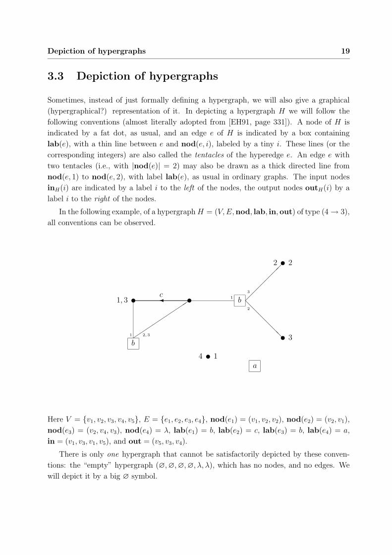
In the following example, of a hypergraph H = (V, E,nod, lab, in,out) of type (4 → 3),
all conventions can be observed.
b
a
bu1, 3 u
u4 1
u2 2
u 3
c
@@
@@
@@1 2, 3
1
3
2
Here V = v1, v2, v3, v4, v5, E = e1, e2, e3, e4, nod(e1) = (v1, v2, v2), nod(e2) = (v2, v1),
nod(e3) = (v2, v4, v3), nod(e4) = λ, lab(e1) = b, lab(e2) = c, lab(e3) = b, lab(e4) = a,
in = (v1, v3, v1, v5), and out = (v5, v3, v4).
There is only one hypergraph that cannot be satisfactorily depicted by these conven-
tions: the “empty” hypergraph (∅,∅,∅,∅, λ, λ), which has no nodes, and no edges. We
will depict it by a big ∅ symbol.
20 I/O-hypergraphs
3.4 Ordinary graphs
Ordinary (directed) graphs, that is hypergraphs where all edges are incident with exactly
two nodes, are special cases of hypergraphs. In other words: a hypergraph over a ranked
alphabet ∆ is an ordinary graph iff for all symbols a ∈ ∆, rank∆(a) = 2. For an ordinary
graph H, an edge e ∈ EH such that nodH(e, 1) = nodH(e, 2) (i.e., both tentacles of e are
incident with the same node) is called a loop.
On ordinary graphs we will define the notion of cutwidth. Let H be an ordinary graph,
and suppose that |VH | = n. Now a bijection f : VH → 1, . . . , n is called a linear layout
of H. A cut is one of the numbers i with 1 ≤ i < n. Intuitively, H is cut between node
f−1(i) and f−1(i + 1)), and by the width of cut i is meant the number of edges that cross
this cut, i.e., those edges e for which either f(nod(e, 1)) ≤ i and f(nod(e, 2)) > i, or
f(nod(e, 2)) ≤ i and f(nod(e, 1)) > i. The cutwidth of H under f , denoted cw(H, f),
is the maximum number of edges e, for all 1 ≤ i < n, for which either f(nod(e, 1)) ≤ i
and f(nod(e, 2)) > i, or f(nod(e, 2)) ≤ i and f(nod(e, 1)) > i. Thus, cw(H, f) is the
maximal width of all cuts. The cutwidth of H, denoted cw(H), is defined as follows:
cw(H) = min( cw(H, f) | f is a linear layout of H ). (3.1)
The following lemma on cutwidth gives as absolute upper bound on the cutwidth of any
given ordinary graph, as a function of the number of nodes it has. For a given ordinary
graph H, over some alphabet ∆, and a linear layout of f of H the cutwidth of H is bounded
by 12
· deg(H) · |VH |:
∀H∈HGR(∆)f :VH→[|VH |]
cw(H, f) ≤1
2· deg(H) · |VH | . (3.2)
The proof is trivial, as obviously cw(H, f) ≤ |EH |, and clearly, by elementary graph theory,
|EH | ≤ 12· deg(H) · |VH |. Therefore, no more than 1
2· deg(H) · |VH | edges can possibly be
cut in any linear layout. This observation immediately leads to the following, somewhat
weaker, lemma:
∀H∈HGR(∆) cw(H) ≤1
2· deg(H) · |VH | . (3.3)
Finally, a linear layout f : VH → 1, . . . , n may intuitively be thought of as the sequence
(f−1(1), . . . , f−1(n)) of all nodes in H.
3.5 String graphs
An ordinary graph where all edges “lie in line” is called a string graph. This is due to
the fact that every string can be uniquely represented as a string graph. For example, the

String graphs 21
string:
abacab
corresponds to the following string graph (i.e. ordinary graph, i.e. hypergraph):
-a -b -a -c -a -bu u u u uu1 u 1
Formally, for an ordinary string w = a1 . . . an over an alphabet Σ, the string graph corre-
sponding with it, denoted gr(w), is defined as follows:
gr(w) = (V, E,nod, lab, in,out),
where V = v0, . . . , vn, E = e1, . . . , en,
nod(ei) = (vi−1, vi) and lab(ei) = ai, for 1 ≤ i ≤ n,
in = (v0),out = (vn).
Note that by this definition, gr(λ) consists of just one node, and no edges (as one would
expect), and:
∀w1,w2∈Σ∗ gr(w1 · w2) = gr(w1) · gr(w2). (3.4)
The function gr : Σ∗ → HGR(Σ) is, as can be easily checked, injective. In other words:
no two different strings are ever mapped to the same string graph, so, as noted, a string
graph uniquely represents a certain string. The degree of a string graph is a direct function
of the length of the underlying string. For a string w:
deg(gr(w)) =
0 if |w| = 0,
1 if |w| = 1,
2 if |w| ≥ 2.
(3.5)
Therefore, a string graph H always has deg(H) ≤ 2. Finally, note that a string graph
never contains a loop, as can be directly seen in the definition.
Now for a class K of hypergraph languages, by STR(K) we denote the class of all
ordinary string languages L such that gr(L) ∈ K:
STR(K) = L |gr(L) ∈ K .
Note that STR(K) is a class of string languages, not hypergraph languages, and fur-
thermore that for every class K of hypergraph languages, and every class K of string
22 I/O-hypergraphs
languages:
STR(gr(K)) = K (3.6)
gr(STR(K)) ⊆ K. (3.7)
3.6 External versus internal nodes
Nodes that are either input nodes, output nodes, or both, are called external nodes. Two
hypergraphs H1 = (V1, E1,nod1, lab1, in1,out), H2 = (V2, E2,nod2, lab2, in2,out2) are
said to be equal modulo i/o, denoted H1 ≡io H2, when V1 = V2, E1 = E2, nod1 = nod2,
and lab1 = lab2. In other words, H1 ≡io H2 holds when H1 is equal to H2, except possibly
for their input or output sequences. Note that ≡io is an equivalence relation, and that in
terms of external nodes a simple hypergraph is just a hypergraph with no external nodes.
This notation is extended to sets of hypergraphs in the following way. For two sets
of hypergraphs L1 and L2 we have L1 ≡io L2 if for every H ∈ L1 there exists a H ′ ∈ L2
such that H ≡io H ′, and, vice versa, for every H ∈ L2 there exists a H ′ ∈ L1 such that
H ≡io H ′.
Nodes that are not external are called internal nodes.
3.7 Hypergraph languages
A hypergraph language over a ranked alphabet ∆ is a set of hypergraphs L ⊆ HGR(∆).
We require that all hypergraphs in L be of type (m → n). L is called of type (m → n).
Like hypergraphs, when L is of type (n → n), it is called of uniform type n. Where
convenient, we will write (L, m → n) instead of just L, to explicitly express the type. The
empty language must have a type too. The empty hypergraph language of type (m → n)
is almost always denoted (∅, m → n) because its type cannot simply be derived from the
hypergraphs within it, as is the case with a nonempty hypergraph language.
The notion of a type extends to classes of hypergraph languages. When a class K of
hypergraph languages only contains hypergraph languages of type (m → n) it is also called
of type (m → n). Otherwise, it is called of mixed type. Note that there is no such thing as
a hypergraph language of mixed type3.
When L contains exactly one hypergraph, it is called a singleton hypergraph lan-
guage. For a set of hypergraphs (not necessarily a hypergraph language) L, Sing(L)
3It is very well possible to put hypergraphs of different types in one set, but that is not a hypergraph
language as far as our definition is concerned.

Union of hypergraph languages 23
denotes the class of all singleton hypergraph languages in P(L): Sing(L) = L′ | L
′ ⊆
L and L′ is a singleton. This class Sing(L) is called the singleton class derived from L.
A hypergraph language L is said to be of bounded degree k if for all graphs H ∈ L, the
degree of H is ≤ k. A hypergraph language L that contains only ordinary graphs, is said
to be of bounded cutwidth k (where k ∈ N) if for all graphs H ∈ L the cutwidth of H is
≤ k.
3.8 Union of hypergraph languages
For two hypergraph languages L1 = (V1, m → n) and L2 = (V2, m → n) of the same type,
the union of both is defined as the hypergraph language L3 = L1 ∪L2 = (V1 ∪V2, m → n).
Note that the resulting hypergraph language is also of type (m → n). The empty language
of type (m → n), (∅, m → n), is the unity element of this union.
Actually we are defining countably infinite union operators: one for every type (m → n).
When convenient, we will write ∪m,n instead of just ∪ to make clear we are applying the
union operator to hypergraph languages of type (m → n).


Text processing has made it possible to
right-justify any idea, even one which
cannot be justified on any other grounds.
— J. Finnigan 4Composition
In this chapter we will define two binary operations on hypergraphs: sequential composition
(the main one), and parallel composition. Using these operations it is possible to take
several hypergraphs and use them to build a larger one.
4.1 Sequential composition
The sequential composition of two hypergraphs H1 and H2, denoted H1 ·H2, is only defined
when #out(H1) = #in(H2). One finds H1 · H2 by first taking the disjoint union of H1
and H2, and then identifying the ith node of outH1 with the ith node of inH2 , for every
1 ≤ i ≤ #out(H1). The resulting graph H1 · H2 has inH1 as input node sequence, and
outH2 as output node sequence. Formally, H1 · H2 is defined as:
((VH1 ∪ VH2)/≡, EH1 ∪ EH2 , (nodH1 ∪ nodH2)≡, labH1 ∪ labH2 , [inH1 ]≡, [outH2 ]≡),
where ≡ is the smallest equivalence relation on VH1 ∪VH2 that contains the following pairs:
(outH1(i), inH2(i)) | 1 ≤ i ≤ #out(H1) .
All this is supposing H1 and H2 are disjoint. If not, we take an isomorphic copy. The
result of the sequential composition of two hypergraphs is also called their product. Note
that the product of two hypergraphs is an ordinary graph iff both hypergraphs are also
ordinary.
25

26 Composition
Actually we are defining countably infinite sequential composition operators: one for
every (m, n, k) ∈ N3. When convenient, we will write ·m,n,k instead of just · to make clear
we are applying the · operator to a H1 of type (m → n) and a H2 of type (n → k), for all
Σ a typed alphabet:
·m,n,k : HGRm,n(Σ) × HGRn,k(Σ) → HGRm,k(Σ).
For every n ∈ N we define a hypergraph Un, called the unity hypergraph of type (n → n):
Un = (v1, . . . , vn,∅,∅,∅, (v1, . . . , vn), (v1, . . . , vn)).
So, for example, U4 is:
u
u
u
u
4 4
3 3
2 2
1 1
Note that Un indeed is of type (n → n), that for every hypergraph H of input type n we
have
Un · H = H, (4.1)
and for every hypergraph G of output type n similarly
G · Un = G. (4.2)
The unity hypergraph of type (0 → 0), U0, is also called the empty hypergraph, for obvious
reasons.
The sequential composition can also be applied to two hypergraph languages, provided
the output type of the first matches the input type of the second. Let L1 = (V1, m → n)
and L2 = (V2, n → k) be hypergraph languages. Now the hypergraph language L3 = L1·L2
is defined as follows:
L3 = (H1 · H2 | H1 ∈ V1, H2 ∈ V2, m → k) . (4.3)
The sequential composition operation is associative, although proving this is surprisingly
hard. Sketch of proof is as follows. Take disjoint hypergraphs H1, H2, and H3. Now by
Sequential composition versus degree and loops 27
completely writing out the expressions H1 · (H2 · H3) and (H1 · H2) · H3 by the definition,
in both cases we arrive at hypergraphs that are isomorphic to:
((VH1 ∪ VH2 ∪ VH3)/≡, EH1 ∪ EH2 ∪ EH3 , (nodH1 ∪ nodH2 ∪ nodH3)≡,
labH1 ∪ labH2 ∪ labH3 , [inH1 ]≡, [outH3 ]≡).
Where ≡ denotes the smallest equivalence relation on VH1 ∪ VH2 ∪ VH3 , that contains the
following pairs:
(outH1(i), inH2(i)) | 1 ≤ i ≤ #out(H1) ,
(outH2(i), inH3(i)) | 1 ≤ i ≤ #out(H2) .
It can be easily seen that in general H1 · H2 6= H2 · H1, so the sequential composition
operation is noncommutative. However, when both H1 and H2 are simple hypergraphs the
sequential composition operation is commutative, as in that case it reduces to just taking
the disjoint union of both hypergraphs.
The symbol∏
stands for a repeatedly applied sequential composition:
n∏
i=1
Hi = H1 . . . Hn, (4.4)
for all n ∈ N, n 6= 0.
Sequential composition is also often called concatenation, because of the analogy with
string concatenation1. We may write the shorthand version H1H2 for H1 · H2.
Because of the associativity of the concatenation we can define Kleene closure on uni-
form hypergraph languages. For a hypergraph language L of uniform type n:
L∗ =
∞⋃
k=0
Lk,
where Lk denotes L, k times concatenated to itself. L
0 denotes the appropriate unity
element, Un in this case. Note that L∗ is again of uniform type n.
4.2 Sequential composition versus degree and loops
Sequential composition can only increase the degree of the hypergraphs involved. Formally
expressed:
∀H1,H2∈HGR(∆)
deg(H1 · H2) ≥ deg(H1),
deg(H1 · H2) ≥ deg(H2).(4.5)
1To summarize: “sequential composition” and “concatenation” are synonyms, and can stand for both
the operation and for the result. The word “product” always denotes the result, and never the operation.
28 Composition
The proof is trivial, as in the process of sequential composition, a node always remains
incident with all the edges it was incident with before. Therefore, the degree of the product
must be at least the degree of the original two hypergraphs. The degree of the product
can be larger, however. This is the case when during identification two or more nodes that
have edges attached to them get merged in such a way that the total degree of the resulting
node is larger than the degree of the original hypergraphs. We can generalize (4.5) to the
product of n hypergraphs in the following way:
∀H1,...,Hn∈HGR(∆) deg
(n∏
i=1
Hi
)
≥ max (deg(Hi) | 1 ≤ i ≤ n ) . (4.6)
Regarding loops, note that by the definition of sequential composition, for hypergraphs
H, H1, H2, such that H = H1 · H2, if H1, or H2, or both, contain a loop, then H itself also
contains a loop.
As a special cases of these properties, for a string graph H, and hypergraphs H1, . . . , Hn,
such that H = H1 . . . Hn, for all Hi, 1 ≤ i ≤ n, deg(Hi) ≤ 2. Proof: as H is a string graph,
deg(H) ≤ 2 (see Section 3.5), and the result directly follows from (4.6). Furthermore, as
H (being a string graph) does not contain a loop, neither does Hi, for 1 ≤ i ≤ n.
4.3 Parallel composition
The parallel composition of two hypergraphs H1 and H2, denoted H1 + H2, is always
defined. One finds H1 + H2 by taking the disjoint union of H1 and H2, and putting
inH1+H2 = inH1 · inH2 and outH1+H2 = outH1 · outH2 . Formally, H1 + H2 is defined as:
(VH1 ∪ VH2 , EH1 ∪ EH2 ,nodH1 ∪ nodH2 , labH1 ∪ labH2 , inH1 · inH2 ,outH1 · outH2),
All this is supposing H1 and H2 are disjoint. If not, we take an isomorphic copy. The
result of the parallel composition of two hypergraphs is called their sum.
The unity element of the parallel composition is the empty hypergraph, U0. It can be
easily verified that for every hypergraph H we have U0 +H = H and likewise H +U0 = H.
The parallel composition acts on unity hypergraphs in the following way:
Un + Um = Un+m. (4.7)
The parallel composition operation is associative. The proof, which directly follows from
the associativity of ∪ and · (on sequences) is very easily accomplished by writing out in
full (H1 + H2) + H3 and H1 + (H2 + H3) where H1, H2, H3 ∈ HGR(Σ) for some Σ, and
H1, H2, H3 mutually disjoint. Both expressions yield the same hypergraph:
(V1∪V2∪V3, E1∪E2∪E3,nod1∪nod2∪nod3, lab1∪lab2∪lab3, in1·in2·in3,out1·out2·out3),

Sequential versus parallel composition 29
which proves the associativity of +.
The parallel composition H1 + H2 is commutative when one or both of H1 and H2 are
simple hypergraphs, but not in general.
The symbol∑
stands for a repeatedly applied parallel composition:
n∑
i=1
Hi = H1 + · · · + Hn, (4.8)
for all n ∈ N, n 6= 0. For the case n = 0 we define∑0
i=1 Hi = U0.
By the associativity of + on both natural numbers and hypergraphs we can now can
generalize (4.7) to:
m∑
k=1
Unk= U(
∑m
k=1nk). (4.9)
The parallel composition can also be applied to two hypergraph languages. Let L1 =
(V1, m1 → n1) and L2 = (V2, m1 → n2) be hypergraph languages. Now the hypergraph
language L3 = L1 + L2 is defined as follows:
L3 = (H1 + H2 | H1 ∈ V1, H2 ∈ V2, m1 + m2 → n1 + n2) .
Note that L3 is by definition of type (m1 + m2 → n1 + n2).
4.4 Sequential versus parallel composition
The basic relationship between the sequential and parallel composition is as follows:
(H1 + H2) · (H ′1 + H ′2) = H1H′1 + H2H
′2, (4.10)
where we require that #outH1 = #inH2 , and #outH1 = #inH2 . Sketch of proof is
as follows. By completely writing out the left-hand and right-hand expression by the
definitions, we arrive in both cases at:
((VH1 ∪ VH2 ∪ VH′
1∪ VH′
2)/≡, EH1 ∪ EH2 ∪ EH′
1∪ EH′
2,
(nodH1 ∪ nodH2 ∪ nodH′
1∪ nodH′
2)/≡, labH1 ∪ labH2 ∪ labH′
1∪ labH′
2,
(inH1 · inH2)/≡, (outH′
1· outH′
2)/≡).
Where ≡ denotes the smallest equivalence relation on VH1 ∪VH2 ∪VH′
1∪VH′
2, that contains
the following pairs:
(outH1(i), inH′
1(i)) | 1 ≤ i ≤ #out(H1)
,

30 Composition
(outH2(i), inH′
2(i)) | 1 ≤ i ≤ #out(H2)
.
All this is, or course, supposing that H1, H2, H ′1, and H ′2 are mutually disjoint. If not, we
take isomorphic copies.
By repeatedly applying (4.10) to itself we get, for all n ∈ N, n ≥ 1:
(H1 + · · · + Hn) · (H ′1 + · · · + H ′n) = H1H′1 + · · · + HnH
′n, (4.11)
under the condition that H1H′1, . . . , HnH
′n are all defined. Proof by induction on n. The
induction basis (n = 1) is trivially fulfilled: (H1) · (H ′1) = H1H′1. Induction step, assuming
the induction hypothesis holds for n = k:
(H1 + · · · + Hk+1) · (H ′1 + · · · + H ′k+1) =(adding parentheses)
((H1 + · · · + Hk) + Hk+1) · ((H ′1 + · · · + H ′k) + H ′k+1)(4.10)=
(H1 + · · · + Hk) · (H ′1 + . . . H ′k) + Hk+1H′k+1 =(induction hypothesis)
(H1H′1 + · · · + HkH
′k) + Hk+1H
′k+1 =(removing parentheses)
H1H′1 + · · · + Hk+1H
′k+1,
which proves (4.11). Note that we can rephrase this equation as:
(n∑
i=1
Hi
)
·
n∑
j=1
H ′j
=n∑
i=1
HiH′i. (4.12)
This relation too can be made more general by repeatedly applying it to itself, which
ultimately gives us the most general case:
m∏
i=1
n∑
j=1
Hij =n∑
j=1
m∏
i=1
Hij. (4.13)
for every m, n ∈ N, m, n ≥ 1. Proof by induction on m (only). Induction basis (m = 1):
1∏
i=1
n∑
j=1
Hij
(4.4)=
n∑
j=1
Hij
(4.4)=
n∑
j=1
1∏
i=1
Hij.
Induction step, assuming the induction hypothesis holds for m = k:
k+1∏
i=1
n∑
j=1
Hij
(4.4)=
k∏
i=1
n∑
j=1
Hij
·n∑
j=1
H(k+1)j =(induction hypothesis)
Expressions used as a function 31
n∑
j=1
k∏
i=1
Hij
·n∑
j=1
H(k+1)j(4.4)=
n∑
j=1
k∏
i=1
Hij
·
n∑
j=1
k+1∏
i=k+1
Hij
(4.12)=
n∑
j=1
(k∏
i=1
Hij
)
·
k+1∏
i=k+1
Hij
(4.4)=
n∑
j=1
k+1∏
i=1
Hij,
which proves (4.13). Note that (4.10) is just the case m = 2, n = 2 of (4.13), and (4.11) is
just the case m = 2.
Furthermore, for simple hypergraphs H1 and H2 we have:
H1 · H2 = H1 + H2.
Finally, the · operator has precedence over the + operator.
4.5 Expressions used as a function
Let H , G : V → HGR(∆) be functions, with a common input domain V , that yield
hypergraphs over some ranked alphabet ∆. We now define two new functions F1, F2 :
V → HGR(∆). For all v ∈ V :
F1(v) = H(v) · G(v),
F2(v) = H(v) + G(v).
In the case that V = HGR(∆) we also define F3, F4, F5, F6 : V → HGR(∆). For all
v ∈ V :
F3(v) = v · H(v),
F4(v) = H(v) · v,
F5(v) = v + H(v),
F6(v) = H(v) + v.
(These six new functions need not be complete.) These constructions deserve their own
notation: we may notate these ad hoc functions F1, . . . , F6 as H ·G, H +G, ·H , H·, +H ,
and H+ respectively. When we consider a hypergraph H ∈ HGR(∆) as a function that
32 Composition
returns H for every v ∈ V , we may now write expressions like “+Un”, the function that
adds the unity hypergraph of uniform order n to its input, or, by recursively applying this
new notation, “(+flip)·backfold”. (flip and backfold are total functions on hypergraphs,
that will be defined in Section 6.1). Finally, we may do the same thing for functions that
yield hypergraph languages.

”What’s one and one and one and one and one
and one and one and one and one and one?”
”I don’t know,” said Alice. ”I lost count.”
— Lewis Carroll 5Decomposition
Sequential and parallel composition are essentially about taking small hypergraphs and
using them to build larger ones. But we can also do the opposite: take a large hypergraph,
and try to break it down in smaller hypergraphs. This process is called decomposition.
In this chapter we will try to find a “small” set of “small” hypergraphs that can be used
to build all other hypergraphs. The result will be useful in defining the class of all “regular”
hypergraph languages (see Chapter 10) and in finding a normal form for interpreters (see
Chapter 7).
5.1 Definition
Let L, L′ ⊆ HGR be sets of hypergraphs. We now write L·
−→ L′, pronounced L decom-
poses sequentially into L′, if for every H ∈ L there exist H1, . . . , Hn ∈ L
′, n ≥ 1, such
that H =∏n
i=1 Hi. In words: every graph H in L can be built from graphs in L′ by just
using sequential composition.
If we also allow parallel composition to be used, we write L·,+−→ L
′, pronounced L fully
decomposes into L′. In words: for every H ∈ L there exist H1, . . . , Hn ∈ L
′ such that H
can be built using just H1, . . . , Hn, ·, and +. Formally: L is a subset of the smallest set of
hypergraphs that contains L′ and is closed under · and +.
It can easily be seen that both·
−→ and·,+−→ are reflexive, transitive relations, and that
sequential decomposition implies full decomposition. In the sections to follow we will
construct sets LA, LB, and LC such that HGR·
−→ LA·
−→ LB·,+−→ LC . The last step will
33

34 Decomposition
involve several substeps.
5.2 HGR ·−→ LA
We define LA as follows:
LA = H ∈ HGR | all nodes v ∈ VH are external .
Now to prove HGR·
−→ LA it suffices to prove that:
∀H∈HGR ∃H1,H2∈LAH = H1 · H2.
For a given H we can always construct such a H1 and H2 by making all nodes in H external,
resulting in H1, and constructing H2 (without edges) in such a way that only the nodes
that are supposed to be external are passed through. Formally, let
H = (V, E,nod, lab, in,out) : p → q.
Furthermore, let v1, . . . , vn be the set of internal nodes of H. We now define:
H1 = (V, E,nod, lab, in,out · (v1, . . . , vn)) : p → q + n,
H2 = (w1, . . . , wq+n,∅,∅,∅, (w1, . . . , wq+n), (w1, . . . , wq)) : q + n → q.
We now have H = H1 · H2.
Example:
Let H be the hypergraph of type (1 → 1), with 2 internal nodes (so p = q = 1 and n = 2),
depicted by:
H = u1
@@
@@
@@
@@
@@R
u
u@
@@
@@
@
@@
@@R
u 1

LA·
−→ LB 35
Then H1 and H2 are of type (1 → 3) and (3 → 1) respectively, and look as follows:
H1 = u1
@@
@@
@@
@@
@@R
u 3
u 2@
@@
@@
@
@@
@@R
u 1 H2 =
u3
u2
u1 1
Note that the edge labels have been left out, as they are irrelevant for the construction.
5.3 LA·−→ LB
We define LB as follows:
LB = H ∈ LA | |EH | ≤ 1 .
Now to prove LA·
−→ LB it suffices to prove that:
∀H∈LA,|EH |>1 ∃H1,H2∈LA(H = H1 · H2 and |EH1 | < |EH | and |EH2 | < |EH |) .
For a given H we can always construct such a H1 and H2 by picking an edge e and reroute
it outside H: H1 ≈ H − e, H2 ≈ e. Formally, let:
H = (V, E,nod, lab, in,out) : p → q,
and choose an edge e ∈ E. Suppose |nod(e)| = n. We now define:
H1 = (V, E − e,nod (E − e), lab (E − e), in,out · nod(e)) : p → q + n,
H2 = (w1, . . . , wq+n, e, e 7→ (wq+1, . . . , wq+n),
e 7→ lab(e), (w1, . . . , wq+n), (w1, . . . , wq)) : q + n → q.
We now have H = H1 · H2, |EH1 | = |EH | − 1 < |EH |, and |EH2 | = 1 < |EH |. This method
to remove an edge by sequential decomposition is called edge removal.
Example:
Let H be the hypergraph, of type (4 → 2) (so p = 4 and q = 2), depicted by:

36 Decomposition
H =
u3
u2, 4
u1
c2
1
b2
PPPPPPPP3
1
a
2
1
u 2
u 1
Then applying edge removal at the edge labeled b (so n = 3), yields the hypergraphs H1
and H2, of type (4 → 5) and (5 → 2) respectively, that look as follows:
H1 =
u3
u2, 4 4
u1
c2
1
a
2
1
u 2, 5
u 1, 3
H2 =
u5
u4
u3
u2 2
u1 1
b
3
2
PPPPPPPP
1
5.4 LB·−→ LC2 ∪ LC3
First we define sets LC1 , LC2 , and LC3 as follows:
LC1 = Ωa | a a ranked symbol ,
LC2 = H ∈ LB | |EH | = 0 ,
LC3 = H ∈ LB | ∃n∈N,a a ranked symbol H = Un + Ωa ,
where Ωa, for rank(a) = n, is defined as follows:
Ωa = (v1, . . . , vn, e, e 7→ (v1, . . . , vn), e 7→ a, (v1, . . . , vn), λ).
For example, when a has rank 5,
Ωa = (v1, v2, v3, v4, v5, e, e 7→ (v1, v2, v3, v4, v5), e 7→ a, (v1, v2, v3, v4, v5), λ) =

LC3
·,+−→ LC1 ∪ LC2 37
u5
u4
u3
u2
u1
aXXXXXXXXXXXX
HHHHHHHHHHHH
5
4
3
2
1
Now to prove LB·
−→ LC2 ∪ LC3 , take an H ∈ LB. If |EH | = 1, sequentially decompose it
into H1 and H2 using edge removal. We now have: H = H1H2, H1 ∈ LC2 and H2 ∈ LC3
(note that H2 = Uq + Ωlab(e), for the q and e as meant in the definition of edge removal).
If |EH | 6= 1, it must be 0, so H ∈ LC2 . This completes the proof.
5.5 LC3
·,+−→ LC1 ∪ LC2
Proof. For all H ∈ LC3 , H = Un + Ωa for some n ∈ N and a a ranked symbol. But
Un ∈ LC2 and Ωa ∈ LC1 , so LC3
·,+−→ LC1 ∪ LC2 . This completes the proof.
5.6 LC2
·,+−→ LC4 ∪ LC5
Define sets LC4 and LC5 as follows:
LC4 = 1m,n | m, n ∈ N, (m, n) 6= (0, 0) ,
LC5 = Ππ,π′,k | π, π′ permutations of (1, . . . , k), k ∈ N .
Here 1m,n is defined as follows:
1m,n = (v,∅,∅,∅, (v, . . . , v)︸ ︷︷ ︸
m times
, (v, . . . , v)︸ ︷︷ ︸
n times
).
For example,
13,2 = (v,∅,∅,∅, (v, v, v), (v, v)) =
u1, 2, 3 1, 2

38 Decomposition
Furthermore, Ππ,π′,k is defined as follows. Suppose π = (i1, . . . , ik) and π′ = (j1, . . . , jk).
Ππ,π′,k = (v1, . . . , vk,∅,∅,∅, (vi1 , . . . , vik), (vj1 , . . . , vjk))
For example,
Π(2,1,3),(3,1,2),3 = (v1, v2, v3,∅,∅,∅, (v2, v1, v3), (v3, v1, v2)) =
u3 1
u1 3
u2 2
This kind of hypergraph is called a permutation hypergraph. Note that it is overkill to
use two permutations, as both can always be combined into one. For technical reasons
however (the symmetry allows us to specify the inverse permutation by swapping π and
π′) we choose to use two.
Choose an H ∈ LC2 . Suppose |VH | = k, V = v1, . . . , vk, and H : m → n. Now H
can always be sequentially decomposed as follows1:
H = Hπ · Hσ · Hπ′ .
Here Hσ : m → n is defined as follows. Let pi indicate the number of occurrences of vi
in inH , and p′i the number of occurrences of vi in outH . Note that for all 1 ≤ i ≤ k,
(pi, pi′) 6= (0, 0) as H ∈ LB.
Hσ =k∑
i=1
1pi,p′
i
This Hσ we now have is almost equal to H, albeit that in and out have been “sorted”:
inHσ= sort(inH) and outHσ
= sort(outH). This is illustrated by the following example:
H = (v1, v2, v3, v4,∅,∅,∅, (v1, v4, v3), (v1, v3, v2, v2)) =
1In order to avoid confusion: the π, π′ and σ in Hπ, Hπ′ and Hσ are just used as a subscript, and have
no meaning of their own. So, the π in Hπ is not a permutation. It is only used to give a hint that Hπ will
be defined as a permutation graph.

LC2
·,+−→ LC4 ∪ LC5 39
u2
u3 2
u 3, 4
u1 1
Now:
Hσ = 11,1 + 10,2 + 11,1 + 11,0
= (v1, v2, v3, v4,∅,∅,∅, (v1, v3, v4), (v1, v2, v2, v3)) =
u3
u2 4
u 2, 3
u1 1
Note that (v1, v3, v4) = sort((v1, v4, v3)) and (v1, v2, v2, v3) = sort((v1, v3, v2, v2)) (where
vi ≤ vj ⇐⇒ i ≤ j). Now consider a permutation (a1, . . . , am) of (1, . . . , m) such that:
inH(a1) ≤ · · · ≤ inH(am),
so we have (inH(a1), . . . , inH(am)) = sort(inH). Similarly, consider a permutation (b1, . . . ,
bn) of (1, . . . , n) such that:
outH(b1) ≤ · · · ≤ outH(bn),
so we have (outH(b1), . . . ,outH(bn)) = sort(outH). Now define Hπ = Π(1,...,m),(a1,...,am),m
and Hπ′ = Π(b1,...,bn),(1,...,n),n. So, continuing the previous example we have: (a1, a2, a3) =
(1, 3, 2) and (b1, b2, b3, b4) = (1, 3, 4, 2)2, and so:
Hπ = (v1, v2, v3,∅,∅,∅, (v1, v2, v3), (v1, v3, v2)),
Hπ′ = (v1, v2, v3, v4,∅,∅,∅, (v1, v3, v4, v2), (v1, v2, v3, v4)).
2Note that these permutations need not be uniquely determined. For example, we could have chosen
(1, 4, 3, 2) instead of (1, 3, 4, 2) for (b1, b2, b3, b4)
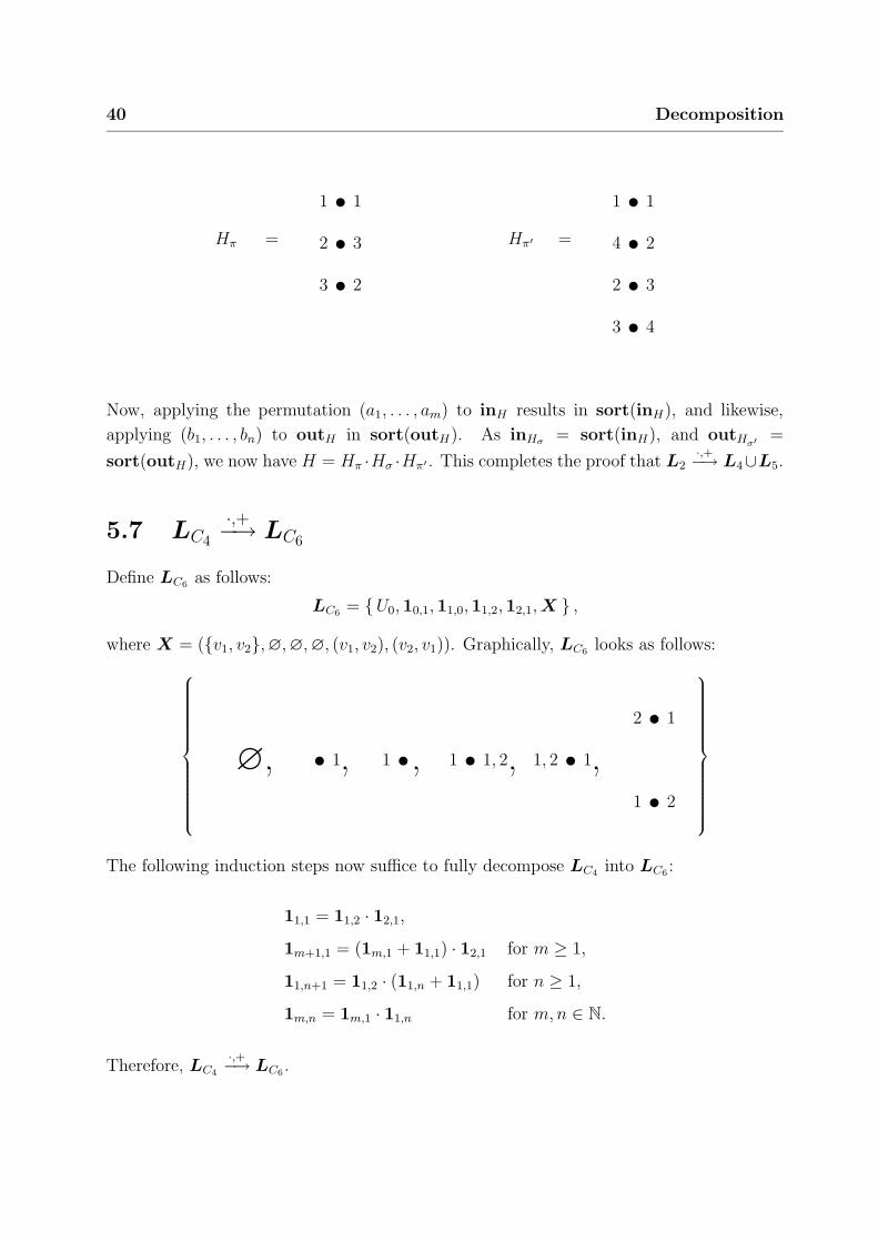
40 Decomposition
Hπ =
u3 2
u2 3
u1 1
Hπ′ =
u3 4
u2 3
u4 2
u1 1
Now, applying the permutation (a1, . . . , am) to inH results in sort(inH), and likewise,
applying (b1, . . . , bn) to outH in sort(outH). As inHσ= sort(inH), and outHσ′
=
sort(outH), we now have H = Hπ ·Hσ ·Hπ′ . This completes the proof that L2·,+−→ L4∪L5.
5.7 LC4
·,+−→ LC6
Define LC6 as follows:
LC6 = U0,10,1,11,0,11,2,12,1, X ,
where X = (v1, v2,∅,∅,∅, (v1, v2), (v2, v1)). Graphically, LC6 looks as follows:
∅, u 1, u1 , u1 1, 2, u1, 2 1,u1 2
u2 1
The following induction steps now suffice to fully decompose LC4 into LC6 :
11,1 = 11,2 · 12,1,
1m+1,1 = (1m,1 + 11,1) · 12,1 for m ≥ 1,
11,n+1 = 11,2 · (11,n + 11,1) for n ≥ 1,
1m,n = 1m,1 · 11,n for m, n ∈ N.
Therefore, LC4
·,+−→ LC6 .

LC5
·,+−→ LC6 41
5.8 LC5
·,+−→ LC6
Choose an H ∈ L5. Suppose |VH | = n. By definition, we now have that outH is a permu-
tation π of inH . From combinatorics/algebra it is well known3 that every permutation π be
can decomposed into permutations π1, . . . , πk where each of the permutations πi only swaps
two neighboring elements. Using these permutations πi we can sequentially decompose H:
H = Π(1,...,n),π,n =k∏
i=1
Π(1,...,n),πi,n.
These hypergraphs Π(1,...,n),πi,n are obviously of the form:
11,1 + · · · + 11,1 + X + 11,1 + · · · + 11,1,
so we have fully decomposed LC5 into LC6 . Therefore, LC5
·,+−→ LC6 . As a consequence of
this, and by the previous sections, LC2
·,+−→ LC6 .
5.9 LB·,+−→ LC
We define LC as follows: LC = LC1 ∪ LC6 . By the transitivity of·,+−→, and because
·−→
implies·,+−→, the results of the previous sections now justify the conclusion LB
·,+−→ LC .
5.10 Conclusions
In trying to decompose HGR a result (not the strongest) we got with sequential decom-
position was
HGR·
−→ LB.
This set LB is called the sequential pseudo base set, because all graphs in HGR can be
built from it, using just sequential composition. Note that it is not finite, and by no means
minimal, as LB can be further sequentially decomposed. (for example to LC2 ∪ LC3 , and
further). For these reason, it is only a pseudo base. There does not exist a “real” sequential
base set (finite, minimal), as HGR contains hypergraphs of type (m → n) for arbitrarily
large m, n ∈ N, and by sequential composition it is not possible to “pump up” the type of
hypergraph.
Using full decomposition we ultimately arrived at
HGR·,+−→ LC .
3See for example Knuth, [Knu73, §5.1], or Herstein, [Her75, §2.10].
42 Decomposition
This set LC is called the full base set because all graphs in HGR can be built from it, using
both sequential and parallel composition. Contrary to the sequential pseudo base set, at
least for a fixed edge label alphabet, the full base set is minimal: it cannot be further
decomposed (into a proper subset). Furthermore, for a fixed edge label alphabet, the full
base set is finite. Formally, by LC “for a fixed edge label alphabet ∆”, we mean LC ∩
HGR(∆). That this set is indeed minimal under this condition can be easily understood
from the following considerations:
• For a fixed label alphabet ∆, all hypergraphs Ωa, for a ∈ ∆, are really needed,
because without all of them, we would be unable to generate hypergraphs that contain
hyperedges labeled a for all a ∈ ∆,
• U0 is really needed, as it obviously cannot be built from any other hypergraph other
than itself,
• 10,1 and 11,0 are really needed, as without them we could not generate edge-less
hypergraphs with internal nodes. Sketch of proof: in all other edge-less hypergraphs
in LC , i.e, U0,11,2,12,1, X, all nodes are both input and output nodes. This prop-
erty clearly remains invariant under both sequential and parallel composition. End
of sketch. That 10,1 and 11,0 are both needed can be shown by similar arguments.
Intuitively, 10,1 and 11,0 are needed to be able to “get rid of external nodes”.
• 11,2 and 12,1 are really needed, as without them we could only generate identification-
free hypergraphs. Sketch of proof: all other hypergraphs in LC are identification-
free, and this property remains invariant under both parallel composition (trivial)
and sequential composition (almost trivial). End of sketch. Again, the fact that 11,2
and 12,1 are both needed can be show by similar arguments.
Intuitively, 11,2 and 12,1 are needed to be able to “split up external nodes”.
• X is really needed, as without it we could only generate hypergraphs H such that
for all 1 ≤ i < j ≤ #in(H), 1 ≤ i′ < j′ ≤ #in(H), such that inH(i) 6= inH(j) and
outH(i′) 6= outH(j′), not both inH(i) = outH(j′) and inH(j) = outH(i′). Sketch
of proof: this property holds for all other hypergraphs in LC , and remains invariant
under both parallel composition (trivial), and sequential composition (almost trivial).
End of sketch.
Intuitively, X is needed to be able to “permute external nodes”.
We do not know whether HGR(∆) can be fully decomposed into another minimal set that
has less elements, but that eventuality seems highly unlikely.
Fold: to bend over or double up so
that one part lies on another part.
— The American Heritage Dictionary 6Folds and flips
In this chapter we will define four natural functions on hypergraphs: fold, backfold, flip,
and split. They exhibit several nice properties that make them very suitable for building
the constructions needed to prove two classes of hypergraph languages equal.
6.1 Definition
Put H = (V, E,nod, lab, in,out) : m → n, and define the following unary operations flip,
fold, backfold, and split on H:
flip(H) = (V, E,nod, lab,out, in) : n → m,
fold(H) = (V, E,nod, lab, λ, in · out) : 0 → m + n,
backfold(H) = (V, E,nod, lab, in · out, λ) : m + n → 0.
Put H = (V, E,nod, lab, (v1, . . . , vm), (vm+1, . . . , vm+n)) : m → n, and define the unary
operation splitp,q on H for all p, q ∈ N, m + n = p + q:
splitp,q(H) = (V, E,nod, lab, (v1, . . . , vp), (vp+1, . . . , vp+q)) : p → q.
Recall that λ denotes the empty sequence, and · denotes the concatenation of sequences.
Note that these operations only manipulate the input and output sequences, the V , E,
nod, and lab components are not changed.
43

44 Folds and flips
We will use the flip, fold, backfold, and split as verbs where convenient, for example
as in “(6.33) is proved by flipping both sides of (6.32)”, i.e., by applying the operation flip
to both sides of the equation.
6.2 Basic properties
These definitions lead to, amongst others, the following properties. Let H be of type
(m → n), and p, q, p′, q′ ∈ N such that p + q = p′ + q′ = m + n.
splitm,n(H) = H, (6.1)
flip(flip(H) = H, (6.2)
flip(fold(H)) = backfold(H), (6.3)
flip(backfold(H)) = fold(H), (6.4)
fold(fold(H)) = fold(H), (6.5)
fold(backfold(H)) = fold(H), (6.6)
fold(splitp,q(H)) = fold(H), (6.7)
backfold(fold(H)) = backfold(H), (6.8)
backfold(backfold(H)) = backfold(H), (6.9)
backfold(splitp,q(H)) = backfold(H), (6.10)
splitp,q(fold(H)) = splitp,q(H), (6.11)
splitp,q(backfold(H)) = splitp,q(H), (6.12)
splitp,q(splitp′,q′(H)) = splitp,q(H). (6.13)
There are no simpler expressions in terms of flip, fold, backfold, and split for the ex-
pressions fold(flip(H)), backfold(flip(H)), splitp,q(flip(H)), and flip(splitp,q(H)). Fur-
thermore we have, directly from the definitions, the following properties:
#in(flip(H)) = #out(H), (6.14)
#out(flip(H)) = #in(H), (6.15)
#in(fold(H)) = 0, (6.16)
#out(fold(H)) = #in(H) + #out(H), (6.17)
#in(backfold(H)) = #in(H) + #out(H), (6.18)
#out(backfold(H)) = 0, (6.19)
#in(splitp,q(H)) = p, (6.20)
Derived properties 45
#out(splitp,q(H)) = q. (6.21)
As previously noted, the flip, fold, backfold, and split operations only manipulate the
input and output sequences (recall from Section 3.6 that ≡io is an equivalence relation):
H ≡io flip(H) ≡io fold(H) ≡io backfold(H) ≡io splitp,q(H). (6.22)
The flip operation is linked to sequential and parallel composition in the following way:
flip(G · H) = flip(H) · flip(G), (6.23)
flip(G + H) = flip(G) + flip(H), (6.24)
flip(Un) = Un. (6.25)
As it turns out, splitp,q can be expressed in terms of fold and backfold, and vice versa.
So, in a sense, either split, or fold and backfold are superfluous. In practice we need
both of them, as some concepts are more elegantly expressed in folds and backfolds, others
in splits. The relations between them are as follows:
fold(H) = split0,#in(H)+#out(H)(H), (6.26)
backfold(H) = split#in(H)+#out(H),0(H), (6.27)
splitp,q(H) = (Up + fold(Uq)) · (backfold(H) + Uq). (6.28)
We extend split to apply to classes of hypergraph languages. Let K be any class of
hypergraph languages.
split(K) = splitp,q(L) | L ∈ K and p, q ∈ N, p + q = #in(L) + #out(L)
(6.29)
Note that now, by (6.26) and (6.27), we have:
fold(K) ⊆ split(K) (6.30)
backfold(K) ⊆ split(K) (6.31)
The above properties are easily verified by expanding the respective definitions.
6.3 Derived properties
A few properties that can be derived from the basic properties are listed below. They
are illustrated in Appendix B, and will be used in Section 8.1 (page 57) and Section 8.2
(page 64) where they are needed in an induction proof.
fold(H2) · (flip(H1) + H3) = fold(H1H2H3), (6.32)

46 Folds and flips
(H1 + flip(H3)) · backfold(H2) = backfold(H1H2H3), (6.33)
both under the condition that H1H2H3 is defined.
(H1 + fold(H3)) · (backfold(H2) + H4) = H1H2H3H4, (6.34)
(fold(H2) + flip(H4)) · (flip(H1) + backfold(H3)) = flip(H1H2H3H4), (6.35)
under the condition that H1H2H3H4 is defined.
(fold(H2) + fold(H4)) · (flip(H1) + backfold(H3) + H5) = fold(H1H2H3H4H5), (6.36)
(H1 + fold(H3) + flip(H5)) · (backfold(H2) + backfold(H4)) = backfold(H1H2H3H4H5),
(6.37)
under the condition that H1H2H3H4H5 is defined.
Note that by flipping both sides of (6.32), (6.34), or (6.36), we get (6.33), (6.35), or
(6.37) respectively, and vice versa. The above six properties can be proved from the basic
properties, albeit in a highly nontrivial way. See also Section B.1.

Be aware of bugs in the above code; I have
only proved it correct, not tried it.
— Donald Ervin Knuth 7Interpretation
In this chapter we devise a method to interpret a string as a hypergraph. As this method
can be extended to interpret string languages as hypergraph languages, and classes of string
languages as classes of hypergraph languages, we can instantly define a lot of classes of
hypergraph languages. For example, from LIN, all linear languages, we instantly derive
Int(LIN), all linear languages under interpretation as hypergraph languages.
7.1 Definition of an interpreter
Let Σ be a typed alphabet, and ∆ a ranked alphabet. Let h be a function, h : Σ →
HGR(∆), that is type preserving, that is, it must satisfy the condition that for every
a ∈ Σ the hypergraph h(a) is of the same type as the symbol a. Let w be a string from
Σ∗, w = a1 . . . an. Now extend h to Σ∗ in the following way: h(w) = h(a1) . . . h(an).
Furthermore, if w = (λ, n → n), we define h((λ, n → n)) as Un. By the definition of h and
· we now have, for all v, w ∈ Σ∗:
h(vw) = h(v)h(w), (7.1)
provided vw is defined. By the associativity of · on both strings and hypergraphs this
generalizes to:
h
(n∏
k=1
wk
)
=n∏
k=1
h(wk), (7.2)
47
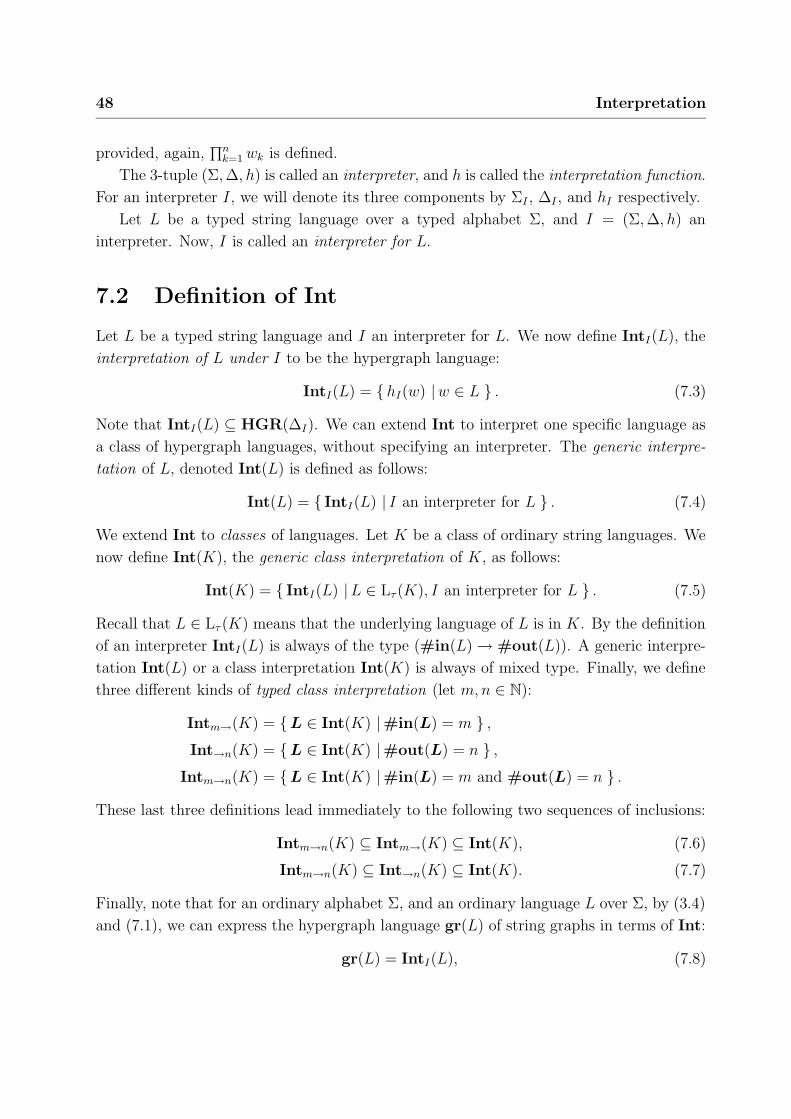
48 Interpretation
provided, again,∏n
k=1 wk is defined.
The 3-tuple (Σ, ∆, h) is called an interpreter, and h is called the interpretation function.
For an interpreter I, we will denote its three components by ΣI , ∆I , and hI respectively.
Let L be a typed string language over a typed alphabet Σ, and I = (Σ, ∆, h) an
interpreter. Now, I is called an interpreter for L.
7.2 Definition of Int
Let L be a typed string language and I an interpreter for L. We now define IntI(L), the
interpretation of L under I to be the hypergraph language:
IntI(L) = hI(w) | w ∈ L . (7.3)
Note that IntI(L) ⊆ HGR(∆I). We can extend Int to interpret one specific language as
a class of hypergraph languages, without specifying an interpreter. The generic interpre-
tation of L, denoted Int(L) is defined as follows:
Int(L) = IntI(L) | I an interpreter for L . (7.4)
We extend Int to classes of languages. Let K be a class of ordinary string languages. We
now define Int(K), the generic class interpretation of K, as follows:
Int(K) = IntI(L) | L ∈ Lτ (K), I an interpreter for L . (7.5)
Recall that L ∈ Lτ (K) means that the underlying language of L is in K. By the definition
of an interpreter IntI(L) is always of the type (#in(L) → #out(L)). A generic interpre-
tation Int(L) or a class interpretation Int(K) is always of mixed type. Finally, we define
three different kinds of typed class interpretation (let m, n ∈ N):
Intm→(K) = L ∈ Int(K) |#in(L) = m ,
Int→n(K) = L ∈ Int(K) |#out(L) = n ,
Intm→n(K) = L ∈ Int(K) |#in(L) = m and #out(L) = n .
These last three definitions lead immediately to the following two sequences of inclusions:
Intm→n(K) ⊆ Intm→(K) ⊆ Int(K), (7.6)
Intm→n(K) ⊆ Int→n(K) ⊆ Int(K). (7.7)
Finally, note that for an ordinary alphabet Σ, and an ordinary language L over Σ, by (3.4)
and (7.1), we can express the hypergraph language gr(L) of string graphs in terms of Int:
gr(L) = IntI(L), (7.8)

Examples of interpretation 49
where I = (Σ′, ∆, h), Σ′ = Σ such that all symbols a ∈ Σ′ have type (1 → 1). Note that
L is correctly typed with respect to Σ′. Furthermore, ∆ = Σ†, and h(a) = gr(a)‡ for all
a ∈ Σ. We can prove (7.8) as follows:
gr(L) =(set theory)
gr(w) | w ∈ L =(rewriting w as symbols)
gr(a1 . . . an) | a1 . . . an ∈ L (3.4)=
gr(a1) . . . gr(an) | a1 . . . an ∈ L =(definition of h)
h(a1) . . . h(an) | a1 . . . an ∈ L (7.2)=
h(a1 . . . an) | a1 . . . an ∈ L =(rewriting symbols as w)
h(w) | w ∈ L (7.3)=
IntI(L).
As a consequence of all this, for all classes K of ordinary string languages:
gr(K) ⊆ Int(K). (7.9)
7.3 Examples of interpretation
In order to understand more clearly what interpretation is all about, let us take a look at
three examples of it. For the sake of simplicity, both only involve ordinary graphs.
Example 1
We define the typed right-linear language L = abnc | n ∈ N , and the interpreter I =
(Σ, ∆, h) for L, where Σ = (a, 1 → 3), (b, 3 → 3), (c, 3 → 1), ∆ = (a, 2), (b, 2), (c, 2)
(note that by the fact that all ranks in ∆ are 2, I will generate ordinary graphs only), and
h defined as depicted hereafter.
h(a) = u 2, 3
u1 1
h(b) =
u3
u2
u1
u 3
u 2
u 1
-c
b
-a
h(c) = u3 1
u1, 2
†Albeit ranked instead of typed. All symbols a ∈ ∆ have rank∆(a) = 2.‡Even though we here seem to be expressing gr in terms of itself, there is really no circularity involved.
We are merely using a finite number of graph constants, namely gr(a) for all a ∈ Σ.
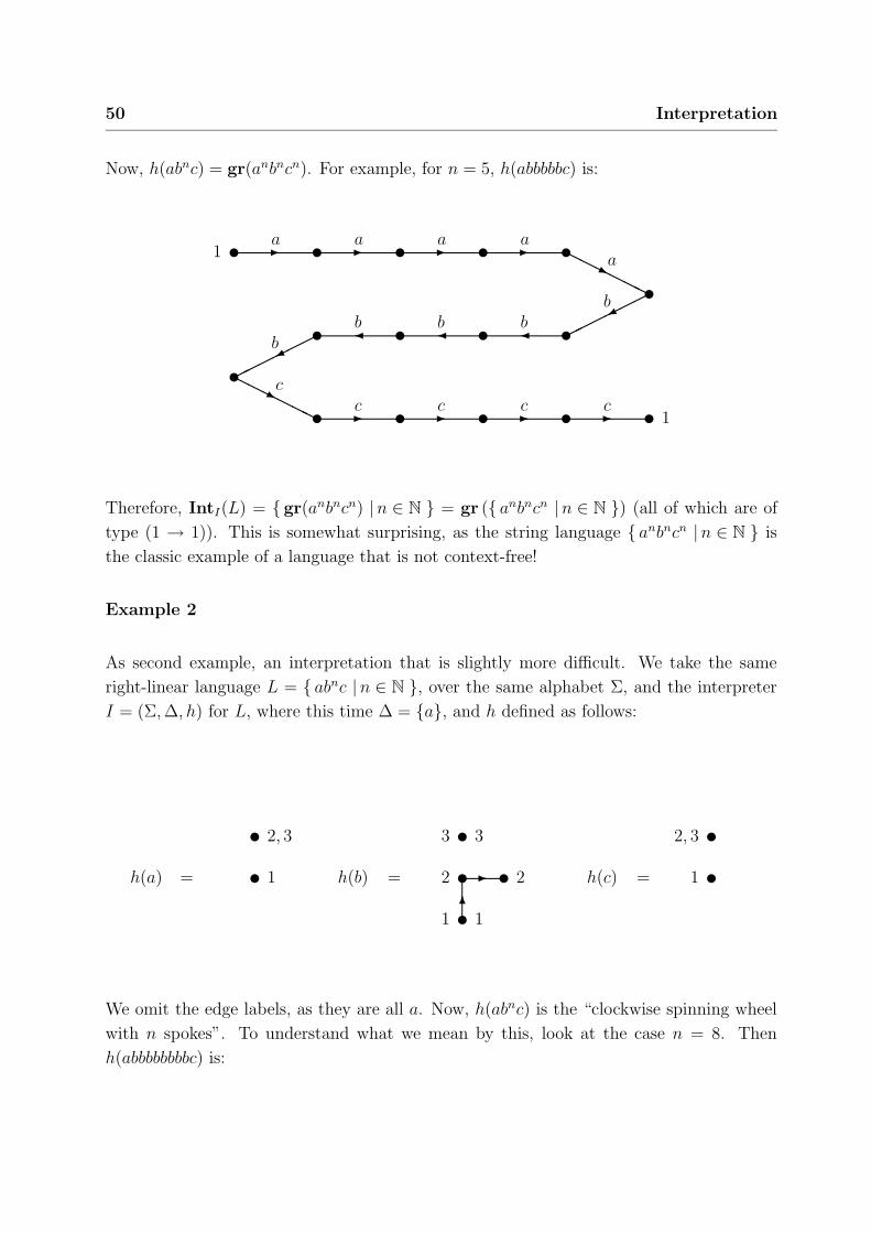
50 Interpretation
Now, h(abnc) = gr(anbncn). For example, for n = 5, h(abbbbbc) is:
u1 -a u -a u -a u -a uHHHHHHja
ububububu
buHHHHHHjc
u -c u -c u -c u -c u 1
Therefore, IntI(L) = gr(anbncn) | n ∈ N = gr ( anbncn | n ∈ N ) (all of which are of
type (1 → 1)). This is somewhat surprising, as the string language anbncn | n ∈ N is
the classic example of a language that is not context-free!
Example 2
As second example, an interpretation that is slightly more difficult. We take the same
right-linear language L = abnc | n ∈ N , over the same alphabet Σ, and the interpreter
I = (Σ, ∆, h) for L, where this time ∆ = a, and h defined as follows:
h(a) = u 1
u 2, 3
h(b) =
u1 1
u2
u3 3
u 2-
6
h(c) = u1
u2, 3
We omit the edge labels, as they are all a. Now, h(abnc) is the “clockwise spinning wheel
with n spokes”. To understand what we mean by this, look at the case n = 8. Then
h(abbbbbbbbc) is:
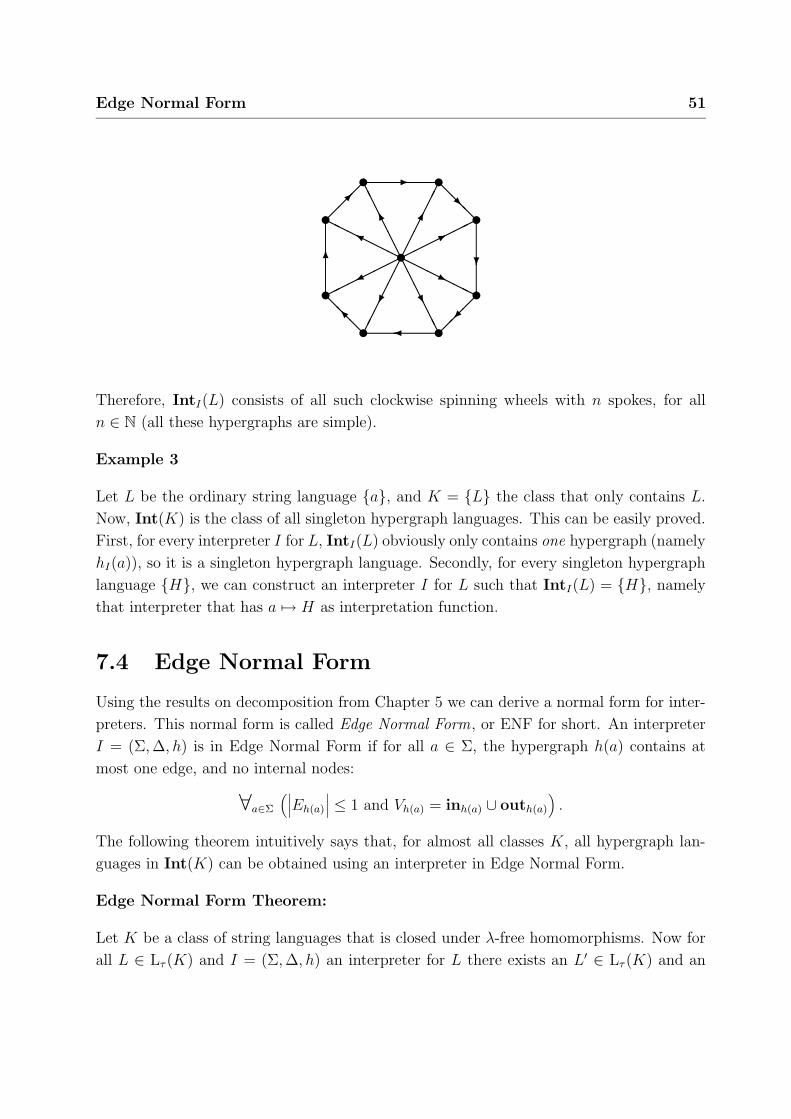
Edge Normal Form 51
uAA
AA
AA
K
*
HHHHHHj
AAAAAA
U
HHHHHHY
u - u@
@@
R u?
u
uu@@
@I
u6
u
Therefore, IntI(L) consists of all such clockwise spinning wheels with n spokes, for all
n ∈ N (all these hypergraphs are simple).
Example 3
Let L be the ordinary string language a, and K = L the class that only contains L.
Now, Int(K) is the class of all singleton hypergraph languages. This can be easily proved.
First, for every interpreter I for L, IntI(L) obviously only contains one hypergraph (namely
hI(a)), so it is a singleton hypergraph language. Secondly, for every singleton hypergraph
language H, we can construct an interpreter I for L such that IntI(L) = H, namely
that interpreter that has a 7→ H as interpretation function.
7.4 Edge Normal Form
Using the results on decomposition from Chapter 5 we can derive a normal form for inter-
preters. This normal form is called Edge Normal Form, or ENF for short. An interpreter
I = (Σ, ∆, h) is in Edge Normal Form if for all a ∈ Σ, the hypergraph h(a) contains at
most one edge, and no internal nodes:
∀a∈Σ
(∣∣∣Eh(a)
∣∣∣ ≤ 1 and Vh(a) = inh(a) ∪ outh(a)
)
.
The following theorem intuitively says that, for almost all classes K, all hypergraph lan-
guages in Int(K) can be obtained using an interpreter in Edge Normal Form.
Edge Normal Form Theorem:
Let K be a class of string languages that is closed under λ-free homomorphisms. Now for
all L ∈ Lτ (K) and I = (Σ, ∆, h) an interpreter for L there exists an L′ ∈ Lτ (K) and an
52 Interpretation
interpreter I ′ = (Σ′, ∆′, h′) for L′ such that I ′ is in ENF and IntI′(L′) = IntI(L).
Proof. As proved in sections 5.2 and 5.3, every hypergraph H can be sequentially decom-
posed in hypergraphs H1, . . . , Hn, where Hi contains at most one edge, and no internal
nodes, for 1 ≤ i ≤ n. For every hypergraph h(a), for a ∈ Σ, choose such a decomposition:
h(a) =na∏
i=1
Ha,i.
Here na denotes the length of the decomposition for h(a). Let 〈a, i〉 denote an element
from the typed alphabet Σ′, which is defined as follows:
Σ′ = 〈a, i〉 | a ∈ Σ and 1 ≤ i ≤ na .
Here the type of a symbol 〈a, i〉 is defined as (#in(Ha,i) → #out(Ha,i)). Now define
the typed language L′ = σ(L) over Σ′, where σ : Σ → Σ′ denotes the following λ-free
homomorphism: for all a ∈ Σ, σ(a) =∏na
i=1〈a, i〉. Define I ′ = (Σ′, ∆′, h′), where ∆′ = ∆,
and for all 〈a, i〉 ∈ Σ′, h′(〈a, i〉) = Ha,i. Note that by this definition (keep in mind the fixed
decompositions) for all a ∈ Σ, h′(σ(a)) = h(a). We now have: IntI′(L′) = IntI(L). Proof:
IntI′(L′)(7.3)=
h′(w) | w ∈ L′ =(definition of L′)
h′(w) | w ∈ σ(L) =(set theory)
h′(σ(v)) | v ∈ L =(definition of h′, σ, and h)
h(v) | v ∈ L (7.3)=
IntI(L).
This completes the proof of the Edge Normal Form theorem.
7.5 Existence of isomorphic copies
In a sense, every hypergraph language that can be obtained by interpretation, can be so
in an infinite number of ways. We will formally express this by the following theorem.
Isomorphic Copies Theorem:
For a class K that is closed under isomorphism, a typed language L ∈ K, and an interpreter
I for L, we can always find an L′ ∈ K, and an interpreter I ′ for L′, such that IntI(L) =
IntI′(L′), and L disjoint with L′.

Bounded degree implies bounded cutwidth 53
Proof. Given a hypergraph language L over a ranked alphabet ∆, a typed string language
L over a typed alphabet Σ, and an interpreter I = (Σ, ∆, h) for L, such that IntI(L) = L,
there exists a typed string language L′ over a typed alphabet Σ′ such that L′ = f(L) for
some isomorphism f , and an interpreter I ′ = (Σ′, ∆′, h′) for L′, such that Σ ∩ Σ′ = ∅ and
IntI′(L′) = L:
∀L∈HGR(∆)L⊆Σ∗
I=(Σ,∆,h)
(IntI(L) = L) =⇒ ∃f :Σ→Σ′ (bijective)L′⊆Σ′∗
I′=(Σ′,∆′,h′)
Σ ∩ Σ′ = ∅ ∧
f(L) = L′ ∧
IntI′(L′) = L
. (7.10)
This can be proved by taking the following Σ′, f , L′, ∆′, and h′:
Σ′ = (a′, m → n) | (a, m → n) ∈ Σ ,
f((a, m → n)) = (a′, m → n), for all (a, m → n) ∈ Σ,
L′ = a′1 . . . a′n | a1 . . . an ∈ L ,
∆′ = ∆,
h′(a′) = h(a).
Obviously L′ = f(L). Now for given L, I, and L such that IntI(L) = L we have:
IntI′(L′)(7.3)=
h′(w′) | w′ ∈ L′ =(rewriting w′ as symbols)
h′(a′1 . . . a′n) | a′1 . . . a′n ∈ L′ (7.2)=
h′(a′1) . . . h′(a′n) | a′1 . . . a′n ∈ L′ =(definition of h, h′, and L′)
h(a1) . . . h(an) | a1 . . . an ∈ L (7.2)=
h(a1 . . . an) | a1 . . . an ∈ L =(rewriting symbols as w)
h(w) | w ∈ L (7.3)=
IntI(L) =(by definition)
L.
This completes the proof of (7.10), from which the Isomorphic Copies Theorem follows as
a corollary.
7.6 Bounded degree implies bounded cutwidth
By the nature of interpretation, some kinds of hypergraph languages are inherently im-
possible to form. As an example of such a limitation, for all IntI(L) that only contain
54 Interpretation
ordinary graphs, we have that if IntI(L) is of bounded degree, necessarily IntI(L) is also
of bounded cutwidth (see Section 3.4):
Degree versus Cutwidth Theorem:
∀ IntI(L) thatonly contain
ordinary graphs
IntI(L) of bounded degree =⇒ IntI(L) of bounded cutwidth. (7.11)
Proof. Denote IntI(L) by L, with L strictly over some typed alphabet Σ, and I = (Σ, ∆, h)
an interpreter for L. Let d be the bound on deg(L), and note that by the definition of
interpretation, the definition of deg(L), and (4.6), now also deg(h(a)) ≤ d for all a ∈ Σ.
Define µ as the maximum number of nodes in any interpreted symbol:
µ = max( ∣
∣∣Vh(a)
∣∣∣
∣∣∣ a ∈ Σ
)
.
Now define the following property P of H ∈ HGR(∆):
P(H)
⇐⇒
There exists a linear layout w1, . . . , wp, wp+1, . . . , wp+q of H (formally: |VH | = p+q for some
p, q ∈ N, and there exists a linear layout f for H such that f(wi) = i for all 1 ≤ i ≤ p + q)
such that the following three conditions hold:
1. cw(H, f) ≤ dµ,
2. w1, . . . , wp = VH − outH ,
3. wp+1, . . . , wp+q = outH .
In words: P(H) means that H has a linear layout with cutwidth ≤ dµ, such that all out
nodes come at the end.
We are now going to prove that:
∀H∈L cw(H) ≤ dµ. (7.12)
Let H ∈ L. If H = Un for some n ∈ N, cw(H) = 0, and we are done (this case arises if
(λ, n → n) ∈ L, because then h((λ, n → n)) = Un). Otherwise, by (7.3) and (7.2), there
exists a string a1 . . . an ∈ L, for some n ≥ 1 such that:
H = h(a1 . . . an) = h(a1) . . . h(an).
Bounded degree implies bounded cutwidth 55
So in order to prove cw(H) ≤ dµ, it suffices to prove P(H), or, P(h(a1) . . . h(an)). We will
prove this by proving the following proposition Q(k), which is defined for 1 ≤ k ≤ n, for
k = n:
Q(k) ⇐⇒ P(h(a1) . . . h(ak)).
We will proceed by induction on k.
Induction basis, k = 1:
Q(1) ( ⇐⇒ P(h(a1))), is trivially fulfilled by (3.2), because deg(h(a1)) ≤ d, and∣∣∣Vh(a1)
∣∣∣ ≤
µ, and therefore cw(h(a1), f) ≤ 12dµ ≤ dµ for any layout f for h(a1). Hence, a layout
where the out nodes of h(a1) come last will satisfy all three conditions in P(h(a1)). Such
a layout obviously exists, which completes the induction basis.
Induction step, k = m + 1:
Assuming Q(m) ( ⇐⇒ P(h(a1) . . . h(am))), where 1 ≤ m < n, we are now going
to prove Q(m + 1) ( ⇐⇒ P(h(a1) . . . h(am+1))). This is done as follows. Note that
h(a1) . . . h(am+1) = (h(a1) . . . h(am)) · h(am+1). Look at the conditions in the definition
of P(h(a1) . . . h(am+1)). Take as linear layout for h(a1) . . . h(am+1) a layout that starts
with w1, . . . , wp as meant in P(h(a1) . . . h(am)). As none of these nodes were out nodes of
h(a1) . . . h(am), no identification has taken place on them during the concatenation with
h(am+1), and consequently no new edges have become incident with them. Therefore, this
first part of the layout still has cutwidth ≤ dµ.
The remainder of the layout can be chosen at wish, under the restriction that the out
nodes of h(am+1) come last. As this second part of the layout contains at most µ nodes (by
the definition of concatenation), and because deg(h(a1) . . . h(am+1)) ≤ d (by (4.6)), there
can be at most dµ edges running either within this second part, or between this second
part and the first part (formally: there can be at most dµ edges that are incident with a
node in the second part). Therefore, the cut between the first and the second part of the
layout, and the cuts within the second part, all have width ≤ dµ.
The layout thus constructed, as can be easily seen, satisfies the conditions in the def-
inition of P(h(a1) . . . h(am+1)). Therefore, P(h(a1) . . . h(am+1)) holds, and consequently
Q(m + 1) holds also. By induction we have now proven that Q(n) holds, and as an imme-
diate consequence cw(H) ≤ dµ. This completes the proof of (7.12), so cw(L) ≤ dµ.
This theorem puts a clear restriction on the kind of hypergraph languages L that can be
generated using interpretation: an L with bounded degree, but no bounded cutwidth is
fundamentally impossible. An example of such a language L is the language of all ordinary

56 Interpretation
graphs that form binary trees. As Lengauer proved in 1982 [Len82], a complete binary tree
of depth 2k has cutwidth k + 1 (for k ≥ 1). As L contains all complete binary trees, this
means that L is not of bounded cutwidth. Since L is of bounded degree, it cannot be
generated by means of interpretation.
As a final remark, let it be noted that something quite similar has been done for eNCE
graph grammars (a node rewriting based approach), by Engelfriet and Leih in 1989 (see
[EL89, §5]).

We will not give formal correctness proofs of
our constructions, because we feel that these
would only obscure the underlying intuitions.
— Joost Engelfriet and George Leih 8Power of interpretation
In this chapter we will examine RLIN, LIN, and DB under interpretation. As it turns
out: Int(RLIN) = Int(LIN) = Int(DB). However, Int(RLIN) Int(CF). We will also
examine Int(STR(Int(K))), and will find that under a few weak conditions on K, it is
equal to Int(K). From these results, we will be able to prove two theorems that nicely
indicate the power of interpretation.
8.1 Int(RLIN) = Int(LIN)
Firstly, to prove Int(RLIN) ⊆ Int(LIN) we only have to observe that RLIN ⊆ LIN. So for
any L ∈ Lτ (RLIN) and I an interpreter for L, there exists an L′ ∈ Lτ (LIN) and an I ′ an
interpreter for L′ such that IntI(L) = IntI′(L′) (namely: L′ = L and I ′ = I). This proves
that Int(RLIN) ⊆ Int(LIN). As a matter of fact this proof extends to any K1 ⊆ K2:
( K1 ⊆ K2 ) =⇒ ( Int(K1) ⊆ Int(K2) ) . (8.1)
Secondly, to prove Int(RLIN) ⊇ Int(LIN) we construct for every L ∈ Lτ (LIN) and I =
(Σ, ∆, h) an interpreter for L an L′ ∈ Lτ (RLIN) and an interpreter I ′ for L′ such that
IntI(L) = IntI′(L′).
Choose a typed linear grammar G = (N, T, P, S) (where T = Σ) such that L(G) = L.
Now construct the following typed right-linear grammar G′ = (N ′, T ′, P ′, S ′), and I ′ an
interpreter for L(G′). Note that from now on we will mostly write h and h′ instead of hI
and h′I respectively, as there can be no confusion.
57
58 Power of interpretation
• I ′ = (Σ′, ∆′, h′), where Σ′ = T ′, ∆′ = ∆, and h′ as defined below.
• N ′ = N ∪ D, D /∈ N ,
For A ∈ N ′, A 6= D, #inN ′(A) = #inN(A)+#outN(A)+#out(L), #outN ′(A) =
#out(L). Furthermore, #inN ′(D) = #in(L), and #outN ′(D) = #out(L),
• T ′ = ap | p ∈ P ∪ b,
• P ′ = p′ | p ∈ P ∪ q.
If p : A → vBw, where A, B ∈ N and v, w ∈ T ∗, then1:
p′ : A → apB,
where h′(ap) = h(v) + flip(h(w)) + U#out(L), #inT ′(ap) = #in(h′(ap)) = #in(v) +
#out(w) + #out(L), and #outT ′(ap) = #out(h′(ap)) = #out(v) + #in(w) +
#out(L).
If p : A → v then:
p′ : A → ap,
where h′(ap) = backfold(h(v)) + U#out(L), #inT ′(ap) = #in(h′(ap)) = #in(v) +
#out(v) + #out(L), and #outT ′(ap) = #out(h′(ap)) = #out(L).
And finally:
q : D → bS,
where h′(b) = U#in(L) + fold(U#out(L)), #inT ′(b) = #in(h′(b)) = #in(L), and
#outT ′(b) = #out(h′(b)) = #in(L) + 2#out(L),
• S ′ = D.
We now claim IntI′(L(G′)) = IntI(L), so L(G′) is the L′ we are looking for. Proof of the
claim by head recursion as follows.
Invariant:
For all H ∈ HGR(∆), A ∈ N , and i ∈ N:
∃v,w∈T ∗
(
G : S ⇒i vAw and H = h(v) + flip(h(w)) + U#out(L)
)
⇐⇒
∃v′∈T ′∗
(
G′ : S ⇒i v′A and H = h′(v′))
.
1Note the λ-case! (See also the footnote on page 14.)

Int(RLIN) = Int(LIN) 59
Proof:
By induction on the length of the derivations (= on i):
Induction basis, i = 0:
G : S ⇒0 S,
v = (λ,#in(L) → #in(L)),
w = (λ,#out(L) → #out(L)),
G′ : S ⇒0 S,
v′ = (λ,#in(L) + 2#out(L) → #in(L) + 2#out(L)).
To prove:
h(v) + flip(h(w)) + U#out(L) = h′(v′).
Proof:
h(v) + flip(h(w)) + U#out(L) =(definition of h)
U#in(L) + flip(U#out(L)) + U#out(L)(6.25)=
U#in(L) + U#out(L) + U#out(L)(4.9)=
U#in(L)+2#out(L) =(definition of h′)
h′(v′).
Induction step (assuming the hypothesis holds for i = n), from left to right, i = n + 1:
Consider a derivation of length n + 1 in G:
G : S ⇒n vAw ⇒1 vuBzw,
where A, B ∈ N , and u, v, w, z ∈ T ∗ with the production p : A → uBz applied in the last
step. By the induction hypothesis, there exists a derivation G′ : S ⇒n v′A, where v′ ∈ T ′∗,
such that:
h′(v′) = h(v) + flip(h(w)) + U#out(L). (8.2)
Let p′ : A → apB be the production of G′ corresponding to p : A → uBz, by the definition
of P ′. We now have:
G′ : S ⇒n v′A ⇒1 v′apB.
To prove:
h′(v′ap) = h(vu) + flip(h(zw)) + U#out(L).

60 Power of interpretation
Proof:
h′(v′ap)(7.1)=
h′(v′) · h′(ap)(8.2)=
(h(v) + flip(h(w)) + U#out(L)) · h′(ap) =(definition of h′(ap))
(h(v) + flip(h(w)) + U#out(L)) · (h(u) + flip(h(z)) + U#out(L))(4.11)=
h(v) · h(u) + flip(h(w)) · flip(h(z)) + U#out(L)(7.1)=
h(vu) + flip(h(w)) · flip(h(z)) + U#out(L)(6.23)=
h(vu) + flip(h(z)h(w)) + U#out(L)(7.1)=
h(vu) + flip(h(zw)) + U#out(L).
A similar proof applies for the direction from right to left. This completes the proof of the
invariant for i = n + 1, and overall proof of the invariant.
Now for any H ∈ IntI(L):
∃v,w,u∈T ∗ G : S ⇒∗ vAw ⇒1 vuw, such that h(vuw) = H,
where A ∈ N , and production p : A → u applied in the last step. Choose such a v, w, u ∈
T ∗. As implied by the invariant:
∃v′∈T ′∗ G′ : S ⇒∗ v′A and h(v) + flip(h(w)) + U#out(L) = h′(v′).
Choose such a v′ ∈ T ′∗. Let p′ : A → ap be the production in P ′ corresponding to p. Then,
G′ : S ⇒∗ v′A ⇒1 v′ap, and:
h′(v′ap)(7.1)=
h′(v′) · h′(ap) =(invariant)
(h(v) + flip(h(w)) + U#out(L)) · h′(ap) =(definition of h′(ap))
(h(v) + flip(h(w)) + U#out(L)) · (backfold(h(u)) + U#out(L))(6.33)=
backfold(h(v)h(u)h(w)) + U#out(L)(7.2)=
backfold(h(vuw)) + U#out(L) =(as h(vuw)=H)
backfold(H) + U#out(L).
And therefore also:
G′ : D ⇒1 bS ⇒∗ bv′A ⇒1 bv′ap,

Int(RLIN) = Int(LIN) 61
and:
h′(bv′ap)(7.1)=
h′(b) · h′(v′ap) =(as by definition h′(b)=U#in(L)+fold(U#out(L)))
(U#in(L) + fold(U#out(L))) · h′(v′ap) =(proven above)
(U#in(L) + fold(U#out(L))) · (backfold(H) + U#out(L))(6.34)=
U#in(L) · H · U#out(L) · U#out(L) =(unity)
H.
This proves that H ∈ IntI′(L′), so IntI(L) ⊆ IntI′(L′). The proof in the other direction,
IntI(L) ⊇ IntI′(L′), works in the same way. This completes the proof of our claim that
IntI(L) = IntI′(L′), and thus also completes the overall proof Int(RLIN) = Int(LIN).
In order to make the construction we used in this proof more clear, we will give an
example.
Example:
Let L be the typed language anbcn | n ∈ N , over the typed alphabet Σ = (a, 1 →
1), (b, 1 → 1), (c, 1 → 1). By elementary formal language theory, this is a linear language
that is not right-linear2. Let I = (Σ, ∆, h) be the interpreter for L defined by Σ as above,
∆ = ((a, 2), (b, 2), (c, 2)), and h = gr. So:
h(a)= u1 -a u 1 h(b)= u1 -b u 1 h(c)= u1 -c u 1
As can be easily seen, for all w ∈ L, h(w) = gr(w), so:
IntI(L) = gr(L) = gr(anbcn) | n ∈ N .
We will now apply the construction given at the beginning of this section to find a typed
right-linear grammar G′ and an interpreter I ′ for L(G′), such that IntI′(L(G′)) = IntI(L).
First, we need to choose a typed linear grammar G = (N, T, P, S) (where T = Σ) such
that L(G) = L. We take:
• N = (S, 1 → 1),
2Standard procedure to prove this: give a linear grammar that generates L, which proves that L is
indeed linear, and then use the pumping lemma to show that L is not regular, i.e., not right-linear.

62 Power of interpretation
• T = Σ = (a, 1 → 1), (b, 1 → 1), (c, 1 → 1),
• P = p1 : S → aSc, p2 : S → b,
• S = S.
The typed right-linear grammar G′ = (N ′, T ′, P ′, S ′) and the interpreter I ′ = (Σ′, ∆′, h′)
for L(G′) are now, following the construction, defined as:
• Σ′ = T ′ (defined below), ∆′ = ∆, and h′ also as defined below,
• N ′ = (S, 3 → 1), (D, 1 → 1),
• T ′ = ap1 , ap2 , b (types will be defined below),
• P ′ = p′1, p′2, q,
p′1 : S → ap1S, where ap1 has type (3 → 3), and h′(ap1) = h(a) + flip(h(c)) + U1:
h′(ap1) =
u1 -a u 1
u2 c u 2
u3 3
p′2 : S → ap2 , where ap2 has type (3 → 1), and h′(ap2) = backfold(h(b)) + U1:
h′(ap2) =
u1 ?bu2
u3 1
q : D → bS, where b has type (1 → 3), and h′(b) = U1 + fold(U1):
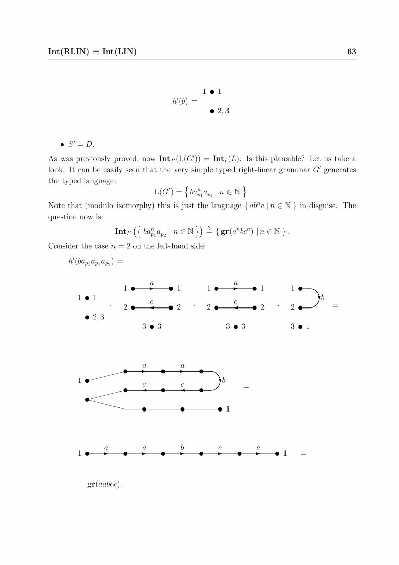
Int(RLIN) = Int(LIN) 63
h′(b) =
u1 1
u 2, 3
• S ′ = D.
As was previously proved, now IntI′(L(G′)) = IntI(L). Is this plausible? Let us take a
look. It can be easily seen that the very simple typed right-linear grammar G′ generates
the typed language:
L(G′) =
banp1
ap2| n ∈ N
.
Note that (modulo isomorphy) this is just the language abnc | n ∈ N in disguise. The
question now is:
IntI′
(
banp1
ap2
∣∣∣ n ∈ N
)?= gr(anbcn) | n ∈ N .
Consider the case n = 2 on the left-hand side:
h′(bap1ap1ap2) =
u1 1
u 2, 3
·
u1 -a u 1
u2 c u 2
u3 3
·
u1 -a u 1
u2 c u 2
u3 3
·
u1 ?bu2
u3 1
=
u1
u -a u -a u ?bucucuu u u u 1
XXXXXX
=
u1 u u u u u 1-a -a -b -c -c =
gr(aabcc).
64 Power of interpretation
N.B.: the thin lines in the above denote that the nodes they connect have been identified.
As we have just shown:
h′(ba2p1
ap2) = h(a2bc2).
Because instead of 2 we could have taken any n ∈ N, this more or less “proves” that
IntI′(L′) = IntI(L). So, yes, the claim is plausible. This concludes the example of the
construction used to prove Int(RLIN) = Int(LIN).
8.2 Int(RLIN) = Int(DB)
Firstly, it is trivial that Int(RLIN) ⊆ Int(DB) because RLIN ⊆ DB (8.1). Secondly,
to prove Int(RLIN) ⊇ Int(DB) we construct for every L ∈ Lτ (DB) and I = (Σ, ∆, h)
an interpreter for L an L′ ∈ Lτ (RLIN) and an interpreter I ′ for L′ such that IntI(L) =
IntI′(L′).
Choose a typed derivation-bounded grammar G = (N, T, P, S) (where T = Σ) such
that L(G) = L. Now construct the following right-linear grammar G′ = (N ′, T ′, P ′, S ′),
where k denotes the derivation bound of G, and I ′ an interpreter for L(G′).
• I ′ = (Σ′, ∆′, h′), where Σ′ = T ′, ∆′ = ∆, and h′ as defined above,
• N ′ =(⋃k
i=1 N ′i)
∪ D, where N ′i = [A1 . . . Ai] | A1, . . . , Ai ∈ N .
Intuitively: there exists a nonterminal in N ′ for every sequence of up to k nonter-
minals in N. Furthermore, there is a new nonterminal D.
The type of [A1 . . . An] ∈ N ′ is:
#inN ′([A1 . . . Am]) =
(m∑
k=1
(#inN(Ak) + #outN(Ak))
)
+ #out(L),
#outN ′([A1 . . . Am]) = #out(L).
Furthermore, #inN ′(D) = #in(L) and #outN ′(D) = #out(L).
• T ′ = ap | p ∈ P ′.
Intuitively: there exists a unique terminal for every production in P ′,
• P ′ =(⋃
p∈P Q(p))
∪ p0.
Intuitively: Q(p) comprises a set of productions that “accomplishes” the same in
G′ as p “accomplishes” in G. This will become clearer after Q(p) has been defined.
Furthermore, there is a production p0. For
p : A0 → v1A1v2A2 . . . vn−1An−1vn, v1, . . . , vn ∈ T ∗, A0, . . . , An−1 ∈ N, n ≥ 1,

Int(RLIN) = Int(DB) 65
Q(p) contains the production q(p, [B1 . . . Bm], i) for every [B1, . . . , Bm] ∈ N ′, and
every i, 1 ≤ i ≤ m, such that A0 = Bi, under the condition that m + n − 2 ≤ k.
The production p′ = q(p, [B1 . . . Bm], i) looks as follows:
[B1 . . . Bm] → ap′ [B1 . . . Bi−1A1 . . . An−1Bi+1 . . . Bm]
N.B.:
1. Should [B1 . . . Bi−1A1 . . . An−1Bi+1 . . . Bm] reduce to “[ ]” because m = 1, n = 1,
and i = 1, we will interpret this as the syntactically empty string (in other
words, we will pretend the [ ] is not there at all). When that happens p′ reduces
to the production [B1] → ap′ .
2. Because m+n−2 ≤ k it is guaranteed that [B1 . . . Bi−1A1 . . . An−1Bi+1 . . . Bm] ∈
N ′ (unless, or course, it reduces to [ ]).
3. This condition m + n − 2 ≤ k is not a restrictive one, as the derivation bound-
edness of G guarantees that there is “no need” for sentential forms that contain
more than k nonterminals.
4. Intuitively the above production rewrites the ith nonterminal according to p.
For this production h′(ap′) is defined as follows3:
h′(ap′) = H(B1)+· · ·+H(Bi−1)+H(v1)+· · ·+H(vn)+H(Bi+1)+· · ·+H(Bm)+U#out(L),
where:
H(Bj) = U#in(Bj)+#out(Bj) for 1 ≤ j ≤ i − 1 or i + 1 ≤ j ≤ m,
H(v1) = backfold(h(v1)) for n = 1,
H(v1) = h(v1) for n ≥ 2,
H(vj) = fold(h(vj)) for n ≥ 2 and 2 ≤ j ≤ n − 1,
H(vn) = flip(h(vn)) for n ≥ 2.
Furthermore, we need to define:
#inT ′(ap′) = #in(h′(ap′)) = (∑m
l=1 (#inN(Bl) + #outN(Bl))) + #out(L),
#outT ′(ap′) = #out(h′(ap′)) =(∑i−1
l=1 (#inN(Bl) + #outN(Bl)))
+(∑n−1
l=1 (#inN(Al) + #outN(Al)))
+(∑m
l=i+1 (#inN(Bl) + #outN(Bl)))
+ #out(L).
3Note the λ-case! (See also the footnote on page 14.)
66 Power of interpretation
And finally:
p0 : D → ap0 [S],
where h′(ap0) = U#in(L) + fold(U#out(L)), #inT ′(ap0) = #in(L), and #outT ′(ap0) =
#in(L) + 2#out(L),
• S ′ = D.
We now have IntI′(L(G′)) = IntI(L), so L(G′) is the L′ we are looking for. Proof by head
recursion as follows:
Invariant:
For all H ∈ HGR(∆), Ai ∈ N , n ≥ 2, and j ∈ N:
∃v1,...,vn∈T ∗
G : S ⇒j v1A1v2 . . . vn−1An−1vn
and
H = h(v1) + fold(h(v2)) + · · · + fold(h(vn−1)) + flip(h(vn)) + U#out(L)
⇐⇒
∃v′∈T ′∗
(
G′ : [S] ⇒j v′[A1 . . . An−1] and H = h′(v′))
.
Proof:
In proving this invariant, we reason along the same lines as we did in the proof in Sec-
tion 8.1. Consequently, we will notate somewhat more tersely now, as there is enough
verbatim correspondence between the two proofs as it is. Induction on the length of the
derivations (= on j):
Induction basis, j=0:
G : S ⇒0 S,
n = 2,
v1 = (λ,#in(L) → #in(L)),
v2 = (λ,#out(L) → #out(L)),
G′ : [S] ⇒0 [S],
v′ = (λ,#in(L) + 2#out(L) → #in(L) + 2#out(L)).
To prove:
h(v1) + flip(h(v2)) + U#out(L) = h′(v′).
Int(RLIN) = Int(DB) 67
Proof:
h(v1) + flip(h(v2)) + U#out(L) =(definition of h)
U#in(L) + flip(U#out(L)) + U#out(L)(6.25)=
U#in(L) + U#out(L) + U#out(L)(4.9)=
U#in(L)+2#out(L) =(definition of h′)
h′(v′).
Induction step, assuming the hypothesis holds for ⇒l, j = l + 1:
Consider a derivation of length l + 1 in G. Such a derivation necessarily consists of a
derivation of length l:
G : S ⇒l v1A1v2 . . . vn−1An−1vn,
followed by a last step in which we apply the production:
p : Ai → w1B1w2 . . . wm−1Bm−1wm.
Firstly, we examine the case where in the last derivation step we are applying a production
that does not have a terminal-only right-hand side (so m ≥ 2), and of that case the subcase
1 < i < n − 1, and n > 2. Then, by the induction hypothesis, there exists a derivation in
G′:
G′ : [S] ⇒l v′[A1 . . . An−1],
such that:
h′(v′) = h(v1) + fold(h(v2)) + · · · + fold(h(vn−1)) + flip(h(vn)) + U#out(L). (8.3)
Let p′ be the production q(p, [A1 . . . An−1], i) of G′ (which corresponds to applying p in the
current context):
p′ : [A1 . . . An−1] → ap′ [A1 . . . Ai−1B1 . . . Bm−1Ai+1 . . . An−1].
Combining these derivations of length l with these last steps, we now have:
G : S ⇒l v1A1v2 . . . vn−1An−1vn ⇒1 v1A1v2 . . . viw1B1w2 . . . wm−1Bm−1wmvi+1 . . . vn−1An−1vn,
G′ : [S] ⇒l v′[A1 . . . An−1] ⇒1 v′ap′ [A1 . . . Ai−1B1 . . . Bm−1Ai+1 . . . An−1].
Note that from the existence of these derivations we can derive, for 1 ≤ r < n:
#in(Ar) = #out(h(vr)),
#out(Ar) = #in(h(vr+1)),(8.4)
68 Power of interpretation
which will come in very handy in our proof.
To prove:
h′(v′ap′) = h(v1) + fold(h(v2)) + · · · + fold(h(vi−1)) +
fold(h(viw1)) + fold(w2) + · · · + fold(wm−1) + fold(h(wmvi+1)) +
fold(h(vi+2)) + · · · + fold(h(vn−1)) + flip(h(vn)) + U#out(L).
Although the expressions in what now follows look quite abhorrent, the steps in between
them are actually very simple. All what happens is some reshuffling of U ’s using (4.9), and
the rewriting of #in(Ai) and #out(Ai), as #out(h(vi)) and #in(h(vi+1)) respectively.
Only in the last step, where we apply (B.2)4, some “real” work is being done.
Proof:
h′(v′ap′)(7.1)=
h′(v′) · h′(ap′)(8.3)=
(h(v1) + fold(h(v2)) + · · · + fold(h(vn−1)) + flip(h(vn)) + U#out(L)) · h′(ap′) =(definition of h′(ap′ ))
(h(v1) + fold(h(v2)) + · · · + fold(h(vn−1)) + flip(h(vn)) + U#out(L)) ·
U#in(A1)+#out(A1) + · · · + U#in(Ai−1)+#out(Ai−1) +
h(w1) + fold(h(w2)) + · · · + fold(h(wm−1)) + flip(h(wm)) +
U#in(Ai+1)+#out(Ai+1) + · · · + U#in(An−1)+#out(An−1) + U#out(L)
(4.9)=
(h(v1) + fold(h(v2)) + · · · + fold(h(vn−1)) + flip(h(vn)) + U#out(L)) ·
U#in(A1)+#out(A1)+···+#in(Ai−1)+#out(Ai−1) +
h(w1) + fold(h(w2)) + · · · + fold(h(wm−1)) + flip(h(wm)) +
U#in(Ai+1)+#out(Ai+1)+···+#in(An−1)+#out(An−1) + U#out(L)
(8.4)=
4The “B” in “(B.2)” refers to Appendix B.
Int(RLIN) = Int(DB) 69
(h(v1) + fold(h(v2)) + · · · + fold(h(vn−1)) + flip(h(vn)) + U#out(L)) ·
U#out(h(v1))+#in(h(v2))+#out(h(v2))+···+#in(h(vi−1))+#out(h(vi−1))+#in(h(vi)) +
h(w1) + fold(h(w2)) + · · · + fold(h(wm−1)) + flip(h(wm)) +
U#out(h(ai+1))+#in(h(vi+2))+#out(h(vi+2))+···+#in(h(vn−1))+#out(h(vn−1))+#in(h(vn)) +
U#out(L)
(4.9)=
(h(v1) + fold(h(v2)) + · · · + fold(h(vn−1)) + flip(h(vn)) + U#out(L)) ·
U#out(h(v1)) + U#in(h(v2))+#out(h(v2)) + · · · + U#in(h(vi−1))+#out(h(vi−1)) +
U#in(h(vi)) + h(w1) + fold(h(w2)) + · · · + fold(h(wm−1)) + flip(h(wm)) + U#out(h(ai+1)) +
U#in(h(vi+2))+#out(h(vi+2)) + · · · + U#in(h(vn−1))+#out(h(vn−1)) + U#in(h(vn)) +
U#out(L)
(B.2)=
h(v1) + fold(h(v2)) + · · · + fold(h(vi−1)) +
fold(h(viw1)) + fold(w2) + · · · + fold(wm−1) + fold(h(wmvi+1)) +
fold(h(vi+2)) + · · · + fold(h(vn−1)) + flip(h(vn)) + U#out(L)
.
The equivalents for the subcases (i = 1 and n > 2), (i = n − 1 and n > 2), and (i = 1 and
n = 2) are not written out in full here, as they are very similar. Most importantly, they
differ in the fact that instead of applying (B.2) in the last step, one needs to apply (B.3),
(B.4), and (B.5) respectively. Note that it is more or less imaginable to combine all these
four cases using a kind meta notation just as in (B.1), but only at the cost of an even more
crippled clarity of the above derivation.
Secondly, we examine the case where in the last derivation step we are applying a produc-
tion that does have a terminal-only right-hand side (so m = 1). We start with the subcase
1 < i < n − 1 and n > 2. This time, we arrive at the following derivations of length l + 1:
G : S ⇒l v1A1v2 . . . vn−1An−1vn ⇒1 v1A1v2 . . . viw1vi+1 . . . vn−1An−1vn,
G′ : [S] ⇒l v′[A1 . . . An−1] ⇒1 v′ap′ [A1 . . . Ai−1Ai+1 . . . An−1].
Note that (8.3) and (8.4) also hold for these derivations.
To prove:
h′(v′ap′) = h(v1) + fold(h(v2)) + · · · + fold(h(vi−1)) + fold(h(viw1vi+1)) +
fold(h(vi+2)) + · · · + fold(h(vn−1)) + flip(h(vn)) + U#out(L).
70 Power of interpretation
Proof (derivation is almost the same as the previous one):
h′(v′ap′)(7.1)=
h′(v′) · h′(ap′)(8.3)=
(h(v1) + fold(h(v2)) + · · · + fold(h(vn−1)) + flip(h(vn)) + U#out(L)) · h′(ap′) =(definition of h′(ap′ ))
(h(v1) + fold(h(v2)) + · · · + fold(h(vn−1)) + flip(h(vn)) + U#out(L)) ·
U#in(A1)+#out(A1) + · · · + U#in(Ai−1)+#out(Ai−1) +
backfold(h(w1)) +
U#in(Ai+1)+#out(Ai+1) + · · · + U#in(An−1)+#out(An−1) + U#out(L)
(4.9)=
(h(v1) + fold(h(v2)) + · · · + fold(h(vn−1)) + flip(h(vn)) + U#out(L)) ·
U#in(A1)+#out(A1)+···+#in(Ai−1)+#out(Ai−1) +
backfold(h(w1)) +
U#in(Ai+1)+#out(Ai+1)+···+#in(An−1)+#out(An−1) + U#out(L)
(8.4)=
(h(v1) + fold(h(v2)) + · · · + fold(h(vn−1)) + flip(h(vn)) + U#out(L)) ·
U#out(h(v1))+#in(h(v2))+#out(h(v2))+···+#in(h(vi−1))+#out(h(vi−1))+#in(h(vi)) +
backfold(h(w1)) +
U#out(h(ai+1))+#in(h(vi+2))+#out(h(vi+2))+···+#in(h(vn−1))+#out(h(vn−1))+#in(h(vn)) +
U#out(L)
(4.9)=
(h(v1) + fold(h(v2)) + · · · + fold(h(vn−1)) + flip(h(vn)) + U#out(L)) ·
U#out(h(v1)) + U#in(h(v2))+#out(h(v2)) + · · · + U#in(h(vi−1))+#out(h(vi−1)) +
U#in(h(vi)) + backfold(h(w1)) + U#out(h(ai+1)) +
U#in(h(vi+2))+#out(h(vi+2)) + · · · + U#in(h(vn−1))+#out(h(vn−1)) + U#in(h(vn)) +
U#out(L)
(B.7)=
h(v1) + fold(h(v2)) + · · · + fold(h(vi−1)) +
fold(h(viw1vi+1)) +
fold(h(vi+2)) + · · · + fold(h(vn−1)) + flip(h(vn)) + U#out(L)

Int(RLIN) = Int(DB) 71
The equivalents for the subcases (i = 1 and n > 2), (i = n − 1 and n > 2), and (i = 1 and
n = 2) are not written out in full here, as they are very similar. Most importantly, they
differ in the fact that instead of applying (B.7) in the last step, one needs to apply (B.8),
(B.9), and (B.10) respectively.
The similar proof applies for the direction from right to left, where we use the same pairs
of derivations for each value of j. This completes the overall proof of the invariant.
Now for any H ∈ IntI(L):5
∃v,w,u∈T ∗ G : S ⇒∗ vAw ⇒1 vuw, such that h(vuw) = H,
where A ∈ N , and production p : A → u applied in the last step. Choose such a v, w, u ∈
T ∗. As implied by the invariant:
∃v′∈T ′∗ G′ : [S] ⇒∗ v′[A] and h(v) + flip(h(w)) + U#out(L) = h′(v′).
Choose such a v′ ∈ T ′∗. Define p′ to be q(p, [A], 1]), the production in P ′ corresponding to
the application of p in the context of [A]. Thus, p′ : [A] → ap′ . Then, G′ : [S] ⇒∗ v′[A] ⇒1
v′ap′ , and:
h′(v′ap′)(7.1)=
h′(v′) · h′(ap′) =(invariant)
(h(v) + flip(h(w)) + U#out(L)) · h′(ap′) =(definition of h′(ap′ ))
(h(v) + flip(h(w)) + U#out(L)) · (backfold(h(u)) + U#out(L))(6.33)=
backfold(h(v)h(u)h(w)) + U#out(L)(7.2)=
backfold(h(vuw)) + U#out(L) =(as by definition h(vuw)=H)
backfold(H) + U#out(L).
And therefore also:
G′ : D ⇒1 ap0 [S] ⇒∗ ap0v′[A] ⇒1 ap0v
′ap′ ,
and:
h′(ap0v′ap′)
(7.1)=
h′(ap0) · h′(v′ap′) =(as by definition h′(ap0 )=U#in(L)+fold(U#out(L)))
(U#in(L) + fold(U#out(L))) · h′(v′ap′) =(as proven above)
5N.B.: this part is almost identical to the last part of Section 8.1.

72 Power of interpretation
(U#in(L) + fold(U#out(L))) · (backfold(H) + U#out(L))(6.34)=
U#in(L) · H · U#out(L) · U#out(L) =(unity)
H.
Which proves that H ∈ IntI′(L′), so IntI(L) ⊆ IntI′(L′). The proof in the other direction,
IntI(L) ⊇ IntI′(L′), works in the same way. This completes the proof of our claim that
IntI(L) = IntI′(L′), and thus also completes the overall proof of Int(RLIN) = Int(DB).
8.3 Int(STR(Int(K))) = Int(K)
Given a class K of string languages, it turns out that under the remarkably weak conditions
that:
• K is closed under λ-free finite substitution, and,
• K is closed under intersection with a regular language,
we have that:
Int(STR(Int(K))) = Int(K). (8.5)
Both RLIN and CF, and most other classes not deliberately constructed to violate these
conditions, can be substituted for K. We will not give a complete formal proof, but only
the construction for a graph language L in the one side of (8.5), given L is contained in
the other side.
Proof. The direction Int(STR(Int(K))) ⊇ Int(K) is easy, as by (7.9) gr(K) ⊆
Int(K), so therefore also STR(gr(K)) ⊆ STR(Int(K)), and by (3.6) K ⊆ STR(Int(K)),
from which the result Int(K) ⊆ Int(STR(Int(K))) immediately follows.
The other direction, Int(STR(Int(K))) ⊆ Int(K), involves a lot of hard work. Given
a hypergraph language L ∈ Int(STR(Int(K))), we construct6 an L′ ∈ Lτ (K), and an
interpreter I ′ = (Σ′, ∆′, h′) for L′, such that IntI′(L′) = L.
Construction:
There exist alphabets Σ1, Σ2, languages L0 ⊆ Σ∗1, L1 ⊆ Σ∗2, with L0 ∈ K, and interpreters
I1 = (Σ1, ∆1, h1), and I2 = (Σ2, ∆2, h2) for L0 and L1 respectively, such that IntI1(L0) =
6Be warned: the construction we give is flooded with technical detail to such an extend, that it borders
on the totally incomprehensible. However, it should be possible to grasp the essence of its inner workings
by studying the explanation that follows the construction.
Int(STR(Int(K))) = Int(K) 73
gr(L1), and IntI2(L1) = L (note that necessarily Σ2 = ∆1, save the types and ranks).
Assume (without loss of generality, as K is closed under λ-free finite substitution) that I1
is in ENF. Define µ to be the maximum input or output type of a h2(a) for all a ∈ Σ2:
µ = max #in(h2(a)),#out(h2(a)) | a ∈ Σ2 .
L′ is formed by applying a λ-free finite substitution to L0, and then intersecting the result
with a regular language:
L′ = σ(L0) ∩ LT .
Here σ is a mapping from Σ1 to finite subsets of Σ′:
σ : Σ1 → P(Σ′),
and LT ⊆ Σ′∗ is a regular language. Σ′ is derived from Σ1:
Σ′ =⋃
a∈Σ1
Σa.
Here, for every symbol (a, m → n) ∈ Σ1, Σa is defined as follows:
Σa =
〈a, 〈i1, . . . , im〉, 〈o1, . . . , on〉〉
∣∣∣∣∣∣
i1, . . . , im, o1, . . . , on ∈ [µ] ∧
P(〈a, 〈i1, . . . , im〉, 〈o1, . . . , on〉〉)
,
where for a = 〈a, 〈i1, . . . , im〉, 〈o1, . . . , on〉〉, and h1(a) = (V, E,nod, lab, in,out), P(a)
denotes the following condition (note that because IntI1(L0) only contains ordinary graphs,
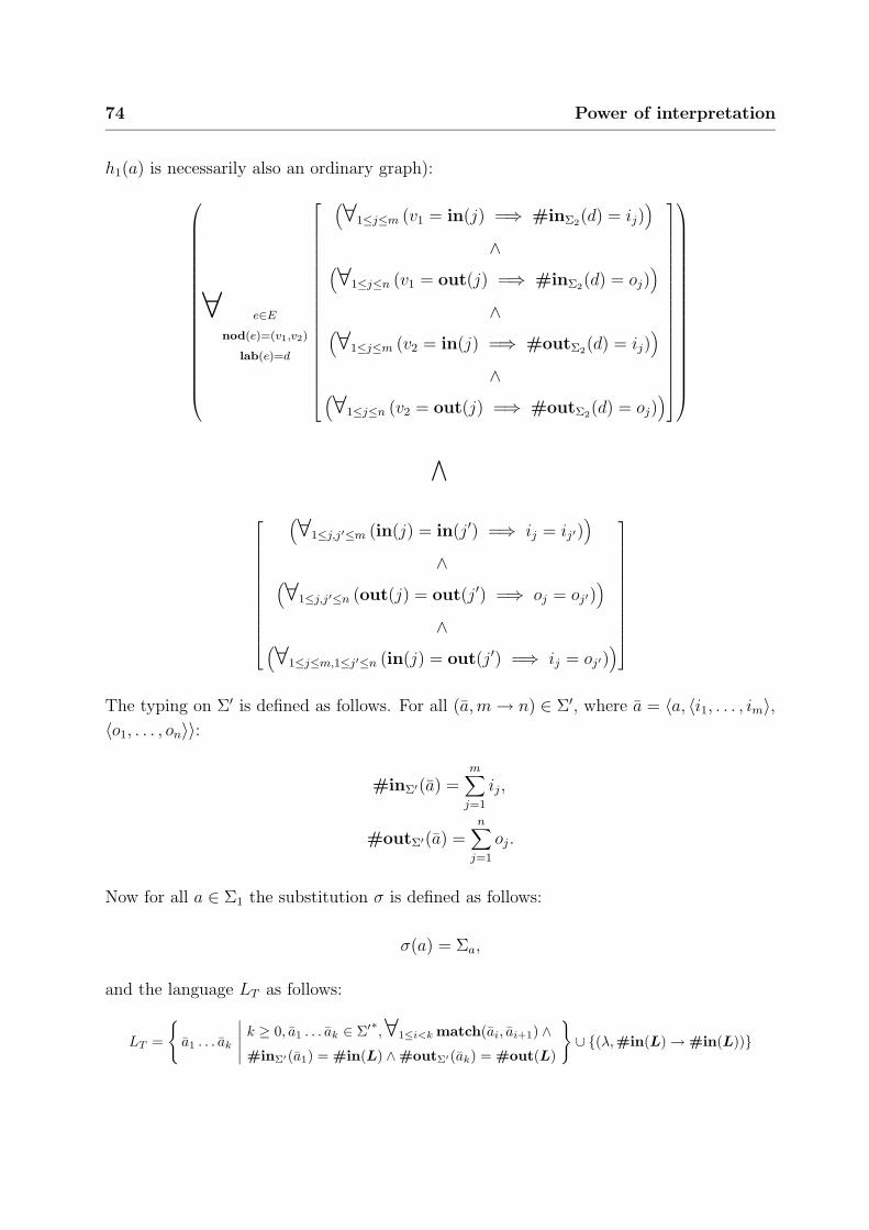
74 Power of interpretation
h1(a) is necessarily also an ordinary graph):
∀ e∈E
nod(e)=(v1,v2)
lab(e)=d
(
∀1≤j≤m (v1 = in(j) =⇒ #inΣ2(d) = ij))
∧(
∀1≤j≤n (v1 = out(j) =⇒ #inΣ2(d) = oj))
∧(
∀1≤j≤m (v2 = in(j) =⇒ #outΣ2(d) = ij))
∧(
∀1≤j≤n (v2 = out(j) =⇒ #outΣ2(d) = oj))
∧
(
∀1≤j,j′≤m (in(j) = in(j′) =⇒ ij = ij′))
∧(
∀1≤j,j′≤n (out(j) = out(j′) =⇒ oj = oj′))
∧(
∀1≤j≤m,1≤j′≤n (in(j) = out(j′) =⇒ ij = oj′))
The typing on Σ′ is defined as follows. For all (a, m → n) ∈ Σ′, where a = 〈a, 〈i1, . . . , im〉,
〈o1, . . . , on〉〉:
#inΣ′(a) =m∑
j=1
ij,
#outΣ′(a) =n∑
j=1
oj.
Now for all a ∈ Σ1 the substitution σ is defined as follows:
σ(a) = Σa,
and the language LT as follows:
LT =
a1 . . . ak
∣∣∣∣∣
k ≥ 0, a1 . . . ak ∈ Σ′∗,∀1≤i<k match(ai, ai+1) ∧
#inΣ′(a1) = #in(L) ∧ #outΣ′(ak) = #out(L)
∪ (λ,#in(L) → #in(L))
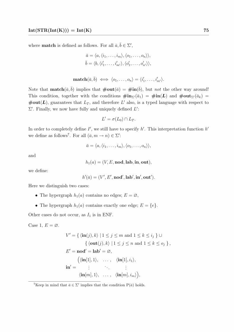
Int(STR(Int(K))) = Int(K) 75
where match is defined as follows. For all a, b ∈ Σ′,
a = 〈a, 〈i1, . . . , im〉, 〈o1, . . . , on〉〉,
b = 〈b, 〈i′1, . . . , i′m′〉, 〈o′1, . . . , o
′n′〉〉,
match(a, b) ⇐⇒ 〈o1, . . . , on〉 = 〈i′1, . . . , i′m′〉.
Note that match(a, b) implies that #out(a) = #in(b), but not the other way around!
This condition, together with the conditions #inΣ′(a1) = #in(L) and #outΣ′(ak) =
#out(L), guarantees that LT , and therefore L′ also, is a typed language with respect to
Σ′. Finally, we now have fully and uniquely defined L′:
L′ = σ(L0) ∩ LT .
In order to completely define I ′, we still have to specify h′. This interpretation function h′
we define as follows7. For all (a, m → n) ∈ Σ′:
a = 〈a, 〈i1, . . . , im〉, 〈o1, . . . , on〉〉,
and
h1(a) = (V, E,nod, lab, in,out),
we define:
h′(a) = (V ′, E ′,nod′, lab′, in′,out′).
Here we distinguish two cases:
• The hypergraph h1(a) contains no edges; E = ∅,
• The hypergraph h1(a) contains exactly one edge; E = e.
Other cases do not occur, as I1 is in ENF.
Case 1, E = ∅.
V ′ = 〈in(j), k〉 | 1 ≤ j ≤ m and 1 ≤ k ≤ ij ∪
〈out(j), k〉 | 1 ≤ j ≤ n and 1 ≤ k ≤ oj ,
E ′ = nod′ = lab′ = ∅,
in′ =
(
〈in[1], 1〉, . . . , 〈in[1], i1〉,...
. . ....
〈in[m], 1〉, . . . , 〈in[m], im〉)
,
7Keep in mind that a ∈ Σ′ implies that the condition P(a) holds.

76 Power of interpretation
out′ =
(
〈out[1], 1〉, . . . , 〈out[1], o1〉,...
. . ....
〈out[n], 1〉, . . . , 〈out[m], on〉)
.
Case 2, E = e,nod(e) = (v1, v2), lab(e) = d. Note that necessarily v1 6= v2, because
otherwise h1(a) would contain a loop, and therefore some H ∈ IntI1(L0) also. As this is a
language of string graphs, this cannot happen (see also Section 4.2).
V ′ = 〈in(j), k〉 | 1 ≤ j ≤ m and 1 ≤ k ≤ ij and in(j) /∈ v1, v2 ∪
〈out(j), k〉 | 1 ≤ j ≤ n and 1 ≤ k ≤ oj and out(j) /∈ v1, v2 ∪
Vh2(d),
E ′ = Eh2(d),
nod′ = nodh2(d),
lab′ = labh2(d),
in′ = in′1 . . . in′m, where:
in′k =
(〈in(k), 1〉, . . . , 〈in(k), ik〉) if in(k) /∈ v1, v2,
inh2(d) if in(k) = v1,
outh2(d) if in(k) = v2.
out′ = out′1 . . . out′n, where:
out′k =
(〈out(k), 1〉, . . . , 〈out(k), ok〉) if out(k) /∈ v1, v2,
inh2(d) if out(k) = v1,
outh2(d) if out(k) = v2.
This fully completes the construction of I ′.
We have now constructed an L′ and an interpreter I ′ for L′, for which we claim that
IntI′(L′) = L. However, we will not give a formal proof of this claim, but instead make it
plausible by explaining how the construction works.
The construction used in this proof is based on the intuition that (8.5):
Int(STR(Int(K))) = Int(K)
holds because we can always “move” an outermost interpretation I2 on the left-hand side
into its corresponding innermost one I1, so that we get an interpretation I ′ that performs
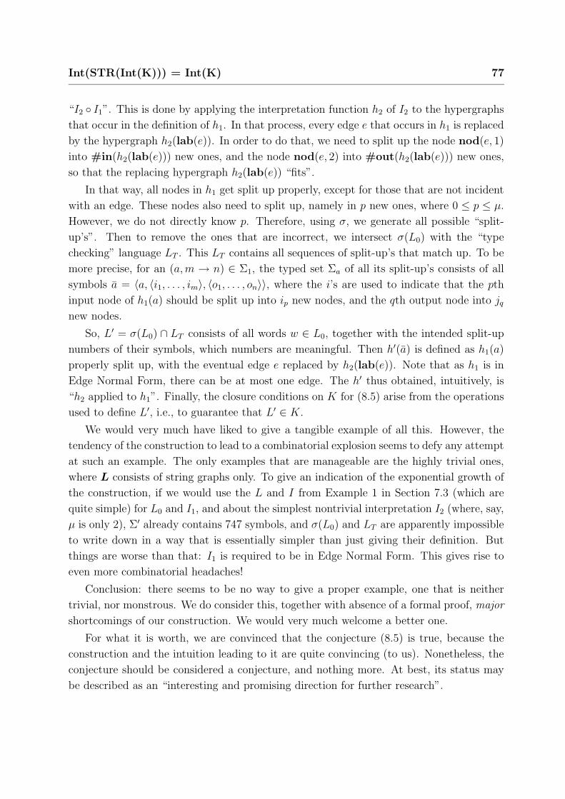
Int(STR(Int(K))) = Int(K) 77
“I2 I1”. This is done by applying the interpretation function h2 of I2 to the hypergraphs
that occur in the definition of h1. In that process, every edge e that occurs in h1 is replaced
by the hypergraph h2(lab(e)). In order to do that, we need to split up the node nod(e, 1)
into #in(h2(lab(e))) new ones, and the node nod(e, 2) into #out(h2(lab(e))) new ones,
so that the replacing hypergraph h2(lab(e)) “fits”.
In that way, all nodes in h1 get split up properly, except for those that are not incident
with an edge. These nodes also need to split up, namely in p new ones, where 0 ≤ p ≤ µ.
However, we do not directly know p. Therefore, using σ, we generate all possible “split-
up’s”. Then to remove the ones that are incorrect, we intersect σ(L0) with the “type
checking” language LT . This LT contains all sequences of split-up’s that match up. To be
more precise, for an (a, m → n) ∈ Σ1, the typed set Σa of all its split-up’s consists of all
symbols a = 〈a, 〈i1, . . . , im〉, 〈o1, . . . , on〉〉, where the i’s are used to indicate that the pth
input node of h1(a) should be split up into ip new nodes, and the qth output node into jq
new nodes.
So, L′ = σ(L0) ∩ LT consists of all words w ∈ L0, together with the intended split-up
numbers of their symbols, which numbers are meaningful. Then h′(a) is defined as h1(a)
properly split up, with the eventual edge e replaced by h2(lab(e)). Note that as h1 is in
Edge Normal Form, there can be at most one edge. The h′ thus obtained, intuitively, is
“h2 applied to h1”. Finally, the closure conditions on K for (8.5) arise from the operations
used to define L′, i.e., to guarantee that L′ ∈ K.
We would very much have liked to give a tangible example of all this. However, the
tendency of the construction to lead to a combinatorial explosion seems to defy any attempt
at such an example. The only examples that are manageable are the highly trivial ones,
where L consists of string graphs only. To give an indication of the exponential growth of
the construction, if we would use the L and I from Example 1 in Section 7.3 (which are
quite simple) for L0 and I1, and about the simplest nontrivial interpretation I2 (where, say,
µ is only 2), Σ′ already contains 747 symbols, and σ(L0) and LT are apparently impossible
to write down in a way that is essentially simpler than just giving their definition. But
things are worse than that: I1 is required to be in Edge Normal Form. This gives rise to
even more combinatorial headaches!
Conclusion: there seems to be no way to give a proper example, one that is neither
trivial, nor monstrous. We do consider this, together with absence of a formal proof, major
shortcomings of our construction. We would very much welcome a better one.
For what it is worth, we are convinced that the conjecture (8.5) is true, because the
construction and the intuition leading to it are quite convincing (to us). Nonetheless, the
conjecture should be considered a conjecture, and nothing more. At best, its status may
be described as an “interesting and promising direction for further research”.
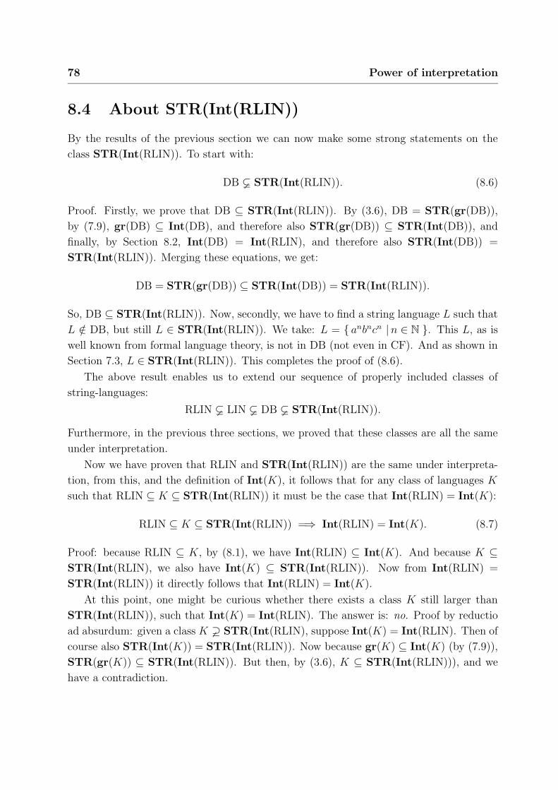
78 Power of interpretation
8.4 About STR(Int(RLIN))
By the results of the previous section we can now make some strong statements on the
class STR(Int(RLIN)). To start with:
DB STR(Int(RLIN)). (8.6)
Proof. Firstly, we prove that DB ⊆ STR(Int(RLIN)). By (3.6), DB = STR(gr(DB)),
by (7.9), gr(DB) ⊆ Int(DB), and therefore also STR(gr(DB)) ⊆ STR(Int(DB)), and
finally, by Section 8.2, Int(DB) = Int(RLIN), and therefore also STR(Int(DB)) =
STR(Int(RLIN)). Merging these equations, we get:
DB = STR(gr(DB)) ⊆ STR(Int(DB)) = STR(Int(RLIN)).
So, DB ⊆ STR(Int(RLIN)). Now, secondly, we have to find a string language L such that
L /∈ DB, but still L ∈ STR(Int(RLIN)). We take: L = anbncn | n ∈ N . This L, as is
well known from formal language theory, is not in DB (not even in CF). And as shown in
Section 7.3, L ∈ STR(Int(RLIN)). This completes the proof of (8.6).
The above result enables us to extend our sequence of properly included classes of
string-languages:
RLIN LIN DB STR(Int(RLIN)).
Furthermore, in the previous three sections, we proved that these classes are all the same
under interpretation.
Now we have proven that RLIN and STR(Int(RLIN)) are the same under interpreta-
tion, from this, and the definition of Int(K), it follows that for any class of languages K
such that RLIN ⊆ K ⊆ STR(Int(RLIN)) it must be the case that Int(RLIN) = Int(K):
RLIN ⊆ K ⊆ STR(Int(RLIN)) =⇒ Int(RLIN) = Int(K). (8.7)
Proof: because RLIN ⊆ K, by (8.1), we have Int(RLIN) ⊆ Int(K). And because K ⊆
STR(Int(RLIN), we also have Int(K) ⊆ STR(Int(RLIN)). Now from Int(RLIN) =
STR(Int(RLIN)) it directly follows that Int(RLIN) = Int(K).
At this point, one might be curious whether there exists a class K still larger than
STR(Int(RLIN)), such that Int(K) = Int(RLIN). The answer is: no. Proof by reductio
ad absurdum: given a class K ! STR(Int(RLIN), suppose Int(K) = Int(RLIN). Then of
course also STR(Int(K)) = STR(Int(RLIN)). Now because gr(K) ⊆ Int(K) (by (7.9)),
STR(gr(K)) ⊆ STR(Int(RLIN)). But then, by (3.6), K ⊆ STR(Int(RLIN))), and we
have a contradiction.
The power of interpretation theorems 79
Combining the above results, for any class K of string languages, we have:
Int(K) ⊆ Int(RLIN) ⇐⇒ K ⊆ STR(Int(RLIN)). (8.8)
The proof is just a recapitulation of earlier proofs in this section. Firstly, the direction =⇒
holds because, as proved in Section 8.3, Int(RLIN) = Int(STR(Int(RLIN))), and hence if
Int(K) ⊆ Int(RLIN), then also K = STR(gr(K)) ⊆ STR(Int(K)) ⊆ STR(Int(RLIN)).
Secondly, the direction ⇐= holds because, if K ⊆ STR(Int(RLIN), then also Int(K) ⊆
Int(STR(Int(RLIN))) = Int(RLIN).
Finally, the class STR(Int(RLIN)) was found to be equal to the class OUT(2DGSM)
by8 Engelfriet and Heyker in 1991.
About this class OUT(2DGSM), the class of all output languages of two-way determin-
istic generalized sequential machines, quite a lot is known; for example, it is a substitution
closed full AFL. For further properties, see [ERS80] and its references.
8.5 The power of interpretation theorems
From the results we have now obtained, we will derive two theorems on the power of
interpretation. Given two classes K and K ′, they give necessary and sufficient conditions
for:
• Int(K) ⊆ Int(K ′), and,
• Int(K) = Int(K ′).
These conditions will be in terms of ordinary string languages only.
Power of Interpretation Theorem I:
For all classes K ′ that are closed under λ-free finite substitution, and under intersection
with a regular language, we have that for any class K:
Int(K) ⊆ Int(K ′) ⇐⇒ K ⊆ STR(Int(K ′)). (8.9)
Proof. As in the proof of (8.8) we did not specifically use properties of RLIN, other
than that it is closed under λ-free finite substitution, and under intersection with a regular
language, we can extend it from RLIN to any class K ′ that satisfies these closure properties.
8See [EH91, page 356], where STR(Int(RLIN)) is called STR(LIN-CFHG). However, beware: their
definition of STR is not identical to ours. See also Section 11.4, where the relation between Int(RLIN)
and LIN-CFHG is discussed (“essentially equal”).

80 Power of interpretation
Power of Interpretation Theorem II:
For all classes K and K ′, such that both are closed under λ-free finite substitution, and
under intersection with a regular language, we have:
Int(K) = Int(K ′) ⇐⇒ STR(Int(K)) = STR(Int(K ′)). (8.10)
Proof. The direction =⇒ is trivial. The direction ⇐= is as follows: if STR(Int(K)) =
STR(Int(K ′)), then obviously also Int(STR(Int(K))) = Int(STR(Int(K ′))). By Sec-
tion 8.3, Int(STR(Int(K))) = Int(K), and Int(STR(Int(K ′))) = Int(K ′), from which
the result then immediately follows.
These two theorem are have clear implications. The second one, intuitively, says that for
two classes of string languages K and K ′, if we want to know whether Int(K) and Int(K ′)
are equal, we just have to check some simple closure properties, and prove the equality for
the string-graph languages in Int(K) and Int(K ′) only.
The first one gives, given a class K ′ that satisfies some closure properties, the largest
class K such that Int(K) is still contained in Int(K ′).
8.6 Conclusions
The results from this chapter give strong indications on the “power” of interpretation. The
fact that Int(RLIN) is equal to Int(DB), although there is quite a gap between RLIN and
DB, tells us that a lot of complexity can be moved out of the interpreted language, into the
interpreter. For example: we can choose a complex language L ∈ DB and any interpreter
I for L, and then construct a simple language L′ ∈ RLIN and an interpreter I ′ for L′ that
generates the same hypergraph language: IntI(L) = IntI′(L′). Somehow the complexity
has “fled” out of L, into I ′!
However, there are limits to the amount of complexity that can be moved in this way.
As we will prove in Section 11.5, Int(CF) is a proper superset of Int(DB). Confusingly
enough, there are languages that are not even context-free, and still under interpretation do
not yield stronger results than RLIN under interpretation (see section 8.4). As an example
of this, take L = anbncn | n ∈ N . As shown in Section 7.3, L ∈ STR(Int(RLIN)). And
by Section 8.3: Int(STR(Int(RLIN))) = Int(RLIN).
This is strange! On the one hand, the class STR(Int(RLIN)) contains a wealth of
complex languages, amongst which all of DB, and even non context-free languages. On the
other hand, all the complexity of Int(STR(Int(RLIN))) can be moved into an interpreter
Conclusions 81
acting on RLIN. Apparently, the complexity of STR(Int(RLIN)) is of a “specific kind”
which can be “handled” by interpretation on RLIN. However, as noted, the complexity of
CF is not of that specific kind, and it can not be handled by interpretation on RLIN. As
a side result of these considerations, by the way, one can easily see that STR(Int(RLIN))
and CF are incomparable, i.e. neither is a subset of the other.
For the case of interpretation on RLIN, we have proven that the kind of complexity inter-
pretation can “cope with”, is exactly the kind of complexity of the class STR(Int(RLIN)).
And in general, for a class K that is closed under λ-free finite substitution, and under inter-
section with a regular language, interpretation on K can exactly cope with the complexity
generated by STR(Int(K)), and nothing more (Power of Interpretation Theorem I).
Furthermore, the Power of Interpretation Theorem II is of great help to prove two
classes equal under interpretation. If for some classes K and K ′ we want to prove that
Int(K) = Int(K ′), essentially all we have to do is to prove it for the string graphs only.
Still a question remains: given a class K, what is the nature of the class STR(Int(K))?
What does it look like? What is its relation with other known classes? As for RLIN, we
know that is leads to OUT(2DGSM). For a similar problem (but beyond the reach of the
formalism of interpretation), Engelfriet and Heyker [EH91, page 355], arrived at the class
OUT(DTWT), all output languages of deterministic tree-walking transducers. Hence, it
seems reasonable to assume STR(Int(K)), for different K, will be equal to other known
classes, and possibly even interesting unknown classes.
Maybe future research will give a more profound insight into the exact nature of
STR(Int(K)), or in other words, into the nature of the complexity interpretation can
cope with. In that way, interpretation might serve as a vehicle to obtain further knowledge
in the field of traditional formal language theory; by taking a detour through the realm of
graph languages, we have found complexity measures on string languages.


A mathematician is a machine for
converting coffee into theorems.
— A. N. Onymous 9Closure properties of Int(K)
In this chapter we will examine the closure properties of Int(K) under several operations.
We will give sufficient conditions for closure in terms of closure properties of K. Sometimes
we can give several, mutually independent, sufficient conditions.
9.1 Closure under sequential composition
Sufficient condition: K closed under concatenation and isomorphism.
Proof. Given two hypergraph languages L1, L2 ∈ Int(K) choose two typed languages
L1, L2 ∈ Lτ (K) over disjoint alphabets (the existence of which is guaranteed by the defini-
tion of Int, the isomorphic copies theorem, and the closure of K under isomorphism), and
two interpreters I1, I2 for L1 and L2 such that IntI1(L1) = L1 and IntI2(L2) = L2.
As K is closed under concatenation we know that L3 = L1 · L2 is in K. Taking
I3 = I1 ∪ I2 (performing the union pairwise on all elements of the 3-tuple) as interpreter
for L3 we get IntI3(L3) = L1 · L2. This is proved as follows:
IntI3(L3)(7.3)=
h3(w) | w ∈ L3 =(definition of L3)
h3(w1 · w2) | w1 ∈ L1, w2 ∈ L2 (7.1)=
h3(w1) · h3(w2) | w1 ∈ L1, w2 ∈ L2 =(definition of h3)
83

84 Closure properties of Int(K)
h1(w1) · h2(w2) | w1 ∈ L1, w2 ∈ L2 (4.3)=
h1(w) | w ∈ L1 · h2(w) | w ∈ L2 (7.3)=
IntI1(L1) · IntI2(L2) =(definition of L1,L2)
L1 · L2.
Therefore, Int(K) is closed under sequential composition. Proving Int(K) closed under
union and Kleene closure works in a similar way. Be warned however: the following two
sections are boringly alike this one!
9.2 Closure under union
Sufficient condition: K closed under union and isomorphism.
Proof. Given two hypergraph languages L1, L2 ∈ Int(K) choose two typed languages
L1, L2 ∈ Lτ (K) over disjoint alphabets (the existence of which is guaranteed by the defini-
tion of Int, the isomorphic copies theorem, and the closure under isomorphism), and two
interpreters I1, I2 for L1 and L2 such that IntI1(L1) = L1 and IntI2(L2) = L2.
As K is closed under union we know that L3 = L1 ∪ L2 is in K. Taking I3 = I1 ∪ I2
(performing the union pairwise on all elements of the 3-tuple) as interpreter for L3 we get
IntI3(L3) = L1 ∪ L2. This is proved as follows:
IntI3(L3)(7.3)=
h3(w) | w ∈ L3 =(definition of L3)
h3(w) | w ∈ L1 ∪ L2 =(set theory)
h3(w) | w ∈ L1 ∪ h3(w) | w ∈ L2 =(definition of h3)
h1(w) | w ∈ L1 ∪ h2(w) | w ∈ L2 (7.3)=
IntI1(L1) ∪ IntI2(L2) =(definition of L1,L2)
L1 ∪ L2.
Therefore, Int(K) is closed under union.
9.3 Closure under Kleene closure
Sufficient condition: K closed under Kleene closure.
Proof. Given a hypergraph language L ∈ Int(K) choose a typed language L ∈ Lτ (K) and
an interpreter I for L, such that IntI(L) = L.

Closure under +Un and Un+ 85
As K is closed under Kleene closure we know that L′ = L∗ is in K. We now have
IntI(L′) = L
∗. This is proved as follows:
IntI(L′)
(7.3)=
h(w) | w ∈ L′ =(definition of L′)
h(w) | w ∈ L∗ (7.2)=
h(w) | w ∈ L ∗ =(definition of L)
L∗.
Therefore, Int(K) is closed under Kleene closure.
9.4 Closure under +Un and Un+
Sufficient condition: TRUE.
Proof. Given a hypergraph language L ∈ Int(K) and an n ∈ N, choose an L ∈ Lτ (K) and
an I = (Σ, ∆, h), an interpreter for L, such that IntI(L) = L. Define I ′ = (Σ′, ∆′, h′) =
(Σ, ∆, h + Un). We now have: IntI′(L) = L + Un. This can be proved as follows:
IntI′(L)(7.3)=
h′(w) | w ∈ L =(rewriting w as symbols)
h′(a1 . . . am) | a1 . . . am ∈ L (7.2)=
h′(a1) . . . h′(am) | a1 . . . am ∈ L =(definition of h′)
(h(a1) + Un) . . . (h(am) + Un) | a1 . . . am ∈ L (4.13)=
(h(a1) . . . h(am)) + (Un . . . Un) | a1 . . . am ∈ L =(unity)
(h(a1) . . . h(am)) + Un | a1 . . . am ∈ L (7.2)=
h(a1 . . . am) + Un | a1 . . . am ∈ L =(rewriting symbols as w)
h(w) + Un | w ∈ L =(definition of +Un)
h(w) | w ∈ L + Un(7.3)=
IntI(L) + Un =(definition of L)
L + Un.
Therefore, Int(K) is closed under +Un. Similarly, we can prove Int(K) to be closed
under Un+.
86 Closure properties of Int(K)
9.5 Closure under parallel composition
Sufficient condition: Int(K) closed under sequential composition. So in terms of a
sufficient condition on K: K closed under concatenation and isomorphism.
Proof. Let L1, L2 ∈ Int(K) be hypergraph languages. We can now derive:
(L1 + U#in(L2)) · (U#out(L1) + L2)(4.10)=
L1 · U#out(L1) + U#in(L2) · L2 =(unity)
L1 + L2.
Because Int(K) is closed under all operations involved (·, +Un, Un+, see sections 9.1
and 9.4) this proves that L1+L2 ∈ Int(K), so Int(K) is closed under parallel composition.
9.6 Closure under fold and backfold
Sufficient condition: fold(Un) ∈ Int(K) (backfold(Un) ∈ Int(K) for closure under
backfold) and Int(K) closed under · and +. So in terms of a sufficient condition on K:
a ∈ K for some symbol a, and K is closed under concatenation and isomorphism.
Proof. Let L ∈ Int(K) be a hypergraph language. We can now derive:
fold(U#in(L)) · (U#in(L) + L)(6.32)=
fold(flip(U#in(L)) · U#in(L) · L)(6.25)=
fold(U#in(L) · U#in(L) · L) =(unity)
fold(L).
Because Int(K) is closed under all operations involved (·, +), and because U#in(L),
fold(U#in(L)) ∈ Int(K) as we can obtain it by interpreting a ∈ K in the appropriate
way, this proves that fold(L) ∈ Int(K), so Int(K) is closed under folding. Proving Int(K)
closed under backfolding works in the same manner, using (6.33) instead of (6.32).
9.7 Closure under flip
Sufficient condition: Un ∈ Int(K) and Int(K) closed under ·, +, fold, and backfold.
So in terms of a sufficient condition on K: a ∈ K for some symbol a, and K is closed
under concatenation and isomorphism.
Closure under flip 87
Proof. Let L ∈ Int(K) be a hypergraph language. We can now derive:
(fold(L) + U#out(L)) · (U#in(L) + backfold(U#out(L)))(6.25)=
(fold(L) + flip(U#out(L))) · (flip(U#in(L)) + backfold(U#out(L)))(6.35)=
flip(U#in(L) · L · U#out(L) · U#out(L)) =(unity)
flip(L).
Because Int(K) is closed under all operations involved (·, +, fold, backfold), and because
U#out(L), U#in(L) ∈ Int(K) as we can obtain them by interpreting a ∈ K in the
appropriate way, this proves that flip(L) ∈ Int(K), so Int(K) is closed under flipping.
However, there is also another, very natural, sufficient condition for closure under flipping:
Sufficient condition: K is closed under reversal.
Proof. Given an L ∈ Int(K), choose an L ∈ Lτ (K) and an I = (Σ, ∆, h), an interpreter
for L, such that IntI(L) = L. As we know that K is closed under reversal, LR ∈ K. Define
I ′ = (Σ′, ∆′, h′) = (Σ, ∆,flip h). We now have: IntI′(LR) = flip(L). This can be proved
as follows:
IntI′(LR)(7.3)=
h′(w)∣∣∣w ∈ LR
=(definition of reversal)
h′(wR) | w ∈ L
=(rewriting w as symbols)
h′(an . . . a1) | a1 . . . an ∈ L (7.2)=
h′(an) . . . h′(a1) | a1 . . . an ∈ L =(definition of h′)
flip(h(an)) . . .flip(h(a1)) | a1 . . . an ∈ L (6.23)=
flip(h(a1) . . . h(an)) | a1 . . . an ∈ L (7.2)=
flip(h(a1 . . . an)) | a1 . . . an ∈ L =(rewriting symbols as w)
flip(h(w)) | w ∈ L =(set theory)
flip ( h(w) | w ∈ L )(7.3)=
flip (IntI(L)) =(definition of L)
flip(L).
Therefore, Int(K) is closed under flipping.

88 Closure properties of Int(K)
9.8 Closure under split
Sufficient condition: Un ∈ Int(K) and Int(K) closed under fold, backfold, · and +.
So in terms of a sufficient condition on K: a ∈ K for some symbol a, and K is closed
under concatenation and isomorphism.
Proof. Let L ∈ Int(K) be a hypergraph language, and p, q ∈ N arbitrary integers such
that p + q = #in(L) + #out(L). We can now derive:
splitp,q(L)(6.28)= (Up + fold(Uq) · (backfold(L) + Uq).
Because Int(K) is closed under all operations involved (fold, backfold, ·, +), and because
Up, Uq ∈ K as we can obtain them by interpreting a ∈ K in the appropriate way,
this proves that splitp,q(L) ∈ Int(K), so Int(K) is closed under splitp,q. As p and q were
arbitrarily chosen, and by (6.29), this means that Int(K) is also closed under split (in
general, without specified p and q).
9.9 Closure under edge relabeling
Sufficient condition: TRUE.
Proof. Let L ∈ Int(K) be a hypergraph language over a ranked alphabet ∆, ∆′ a ranked
alphabet, and f : ∆ → ∆′ a rank preserving function (∀a∈∆ rank(f(a)) = rank(a)).
Extend f in the obvious way to operate on hypergraphs, such that it returns the same
hypergraph, only with the edges relabeled. Now choose a language L ∈ Lτ (K) and I =
(Σ, ∆, h) an interpreter for L such that IntI(L) = L. If we now choose I ′ = (Σ, ∆′, f
h), then clearly IntI′(L) is the hypergraph language that results from applying the edge
relabeling f to (the edge labels in) L. Therefore, Int(K) is closed under the relabeling of
edges.
9.10 Conclusions
Summarizing the results from this chapter, we can draw the following table to express
the sufficient conditions for closure of Int(K). Each row indicates for a certain operation
which closure conditions on K are sufficient to guarantee closure on Int(K) under that
operation. Needed conditions are marked by a bullet (•), “edge relab.” stands for edge
relabeling, and “isomorph” for isomorphism.

Conclusions 89
· ∪ ∗ isomorph a ∈ K reversal
· • •
+ • •
∪ • •∗ •
+Un
Un+
fold • • •
backfold • • •
splitp,q • • •
flip • • •
flip •
edge relab.
Finally, note that RLIN and CF satisfy all mentioned closure conditions. Therefore, both
Int(RLIN) and Int(CF) are closed under all mentioned operations.


If you cannot convince them, confuse them.
— Harry S. Truman 10Another characterization
It turns out that there is another beautiful way to characterize the class of hypergraph
languages Int(RLIN), without the concept of “interpreting” at all! This characterization
is as follows:
Int(RLIN) is the smallest class of hypergraph languages that is closed
under concatenation, parallel composition, union, and Kleene closure, and
that contains the singleton class derived from the full base set.
Before we will be able to prove this characterization, we will first prove that some other
characterizations that look like it also define the class Int(RLIN).
10.1 Using HGR
To begin with, we characterize Int(RLIN) as the smallest class of hypergraph languages
that is closed under concatenation, union, and Kleene closure, and that contains all single-
ton hypergraph languages. To prove that this characterization indeed defines the class
Int(RLIN), we need to prove three things. Firstly, by Section 9.10, it is clear that
Int(RLIN) is indeed closed under concatenation, union, and Kleene closure. Secondly,
it is trivial that Int(RLIN) contains all singleton hypergraph languages, as Int(a)
consists of exactly all singleton hypergraph languages (see Example 3 of Section 7.3), and
clearly a ∈ RLIN. Therefore by (8.1), Int(a) ⊆ Int(RLIN). The third (and last)
part is the hardest: Int(RLIN) is the smallest class that is closed under concatenation,
91
92 Another characterization
Kleene closure, and union, and that contains all singleton hypergraph languages. In order
to prove this, we have to show that every hypergraph language L ∈ Int(RLIN) over some
alphabet ∆ can be denoted by a finite expression over Sing(HGR(∆)), ·, ∗, and ∪ (also
called a regular expression).
Proof. Choose such an L ∈ Int(RLIN). Let L be a typed right-linear language over
some alphabet Σ, and I = (Σ, ∆, h) an interpreter for L, such that IntI(L) = L. From
formal language theory, it is a well known fact1 that L can be expressed by a regular
expression over ·, ∗, ∪, and Σ. So, let r be a regular (string) expression that denotes L.
Now let r′ be the regular (graph) expression derived from r by replacing every occurrence
of a by h(a), for all a ∈ Σ. As we know that for all string languages L′ and L′′:
• if L′ · L′′ is typed, then so are L′ and L′′,
• if L′∗ is typed, then so is L′,
• if L′ ∪ L′′ is typed, then so are L′ and L′′,
• h(L′ · L′′) = h(L′) · h(L′′),
• h(L′∗) = h(L′)∗,
• h(L′ ∪ L′′) = h(L′) ∪ h(L′′),
this proves that r′ = h(r) (by induction on the length of r). Because h(r) = IntI(L) = L,
the regular expression r′ thus obtained denotes the language L. This completes the proof
that every language L ∈ Int(RLIN) can be denoted by a regular expression. Together with
the first two parts, this third part concludes the overall proof that the new characterization
indeed exactly characterizes the class Int(RLIN) we already know.
10.2 Using the sequential pseudo base set
Having obtained the result of the previous section, we can easily make it stronger by using
the results from Chapter 5. In this way, we can characterize Int(RLIN) as the smallest class
of hypergraph languages that is closed under concatenation, union, and Kleene closure, and
that contains the singleton class derived from the sequential pseudo base set. In addition
to what we already proved in the previous section, it now suffices to only prove that every
singleton language in HGR can be represented by an expression over the sequential pseudo
base set and sequential composition. Or, formally expressed, HGR·
−→ LB. But this we
have already proved in Section 5.10, so we are done.
1See for example Hopcroft and Ullman [HU79, §2.5], or Carroll and Long [CL89, §6.2].
Using the full base set 93
Recall that the sequential pseudo base set contains exactly all hypergraphs that have
at most one edge. So, intuitively, this characterization says that Int(RLIN) is the smallest
class of hypergraph languages that is closed under concatenation, union, and Kleene clo-
sure, and that contains all singleton hypergraph languages H where H has zero or one
edges.
10.3 Using the full base set
The same as in the previous section can be done for the full base set. Now, we characterize
Int(RLIN) as the smallest class of hypergraph languages that is closed under concatenation,
parallel composition, union, and Kleene closure, and that contains the singleton class
derived from the full base set (this is the same characterization as given at the beginning of
this chapter). The additionally needed proof follows directly from the fact that Int(RLIN)
is closed under parallel composition (Section 9.5), and HGR·,+−→ LC .
Recall that the full set consists of all “edges” and six “auxiliary hypergraphs”. So,
intuitively, this characterization says that Int(RLIN) is the smallest class of hypergraph
languages that is closed under concatenation, parallel composition, union, and Kleene
closure, and that contains all “edges” (and a few auxiliary hypergraphs).
10.4 Conclusions
There is strong resemblance between the characterization given at the beginning of this
chapter, and the characterization (from formal language theory) of RLIN as the smallest
class that is closed under concatenation, union, and Kleene closure, and that contains all
“symbols” (i.e., languages of the form a, where a is a symbol). Just as that characteriza-
tion intuitively says “the class of regular string languages can be build by regular expres-
sions over the basic building blocks, namely symbols”, ours says “the class Int(RLIN) can
be build by regular expressions over the basic building blocks, namely edges”. We think
that because of this resemblance, Int(RLIN) deserves to be called “the class of regular
graph languages”.


There’s too many men, too many people,
making too many problems. Can’t you
see this is a land of confusion?
— Phil Collins 11Other literature
More than 20 years ago, the concept of a graph grammar was introduced by A. Rosenfeld
as a formulation of some problems in pattern recognition and image processing, as well as
by H. J. Schneider in Germany as a method for data type specification. In this chapter
we will make a comparison between our Int(K) classes of hypergraph languages, and
some classes of hypergraph languages generated by graph grammars on which results have
been published in the scientific literature. In particular we will find that Int(RLIN) ≈
LIN-CFHG1, where LIN-CFHG is the class of (languages generated by) linear context-free
hypergraph grammars, as defined by Engelfriet and Heyker.
11.1 Introduction
Be aware that there is no universally, or even widely, agreed on concept of the “right” way
to define a graph grammar. Instead, there are many fundamentally different approaches.
For example: what should nonterminals stand for, nodes, edges, or perhaps even something
else? As a consequence of this controversy, seemingly simple questions like “what is context
freeness with regard to a graph grammar?” have no conclusive answer (yet).
Although our means of defining hypergraph languages by interpretation has strictly
spoken little or nothing to do with a graph grammar, a string grammar/interpreter pair
1We write ≈ instead of = because their hypergraphs have only one sequence of external nodes, while
ours have two. Except for that small matter, both classes are completely identical. We will turn this into
a precise formal statement, and prove it, in Section 11.4.
95
96 Other literature
is, in our view, a “graph grammar in disguise”. Not surprisingly, some of our results (for
example, our claim that the class Int(RLIN) deserves to be called “the class of regular
graph languages”, and the decomposition of HGR(∆) in a base set) are strikingly similar
to some results derived using a hyper-edge replacement graph grammar approach. Hence
the title of this thesis: “Graphs Grammars and Operations on Graphs”.
In what follows, we will make comparisons to work of Engelfriet and Heyker ([EH91],
[EH92]), Bauderon and Courcelle ([BC87]), and Habel and Kreowski ([Hab92]), all of which
are hyper-edge replacement oriented approaches.
No comparison whatsoever is made with node-replacement oriented approaches. It
may be interesting to observe that node replacement is in general more powerful than edge
replacement. For example, the set of all complete graphs can easily be generated by a node-
replacement graph grammar, but not by means of the above mentioned edge-replacement
graph grammars.
For an overview of developments in the field, recent proceedings of the “International
Workshop on Graph Grammars and Their Application to Computer Science” ([ENRR87],
[EKR91]) are a good place to start.
11.2 Engelfriet and Heyker
The class Int(RLIN) we defined is very similar to the class LIN-CFHG defined by Engelfriet
and Heyker in 1991 [EH91]. Before we can make precise statements, however, we need a
way to “translate” their notion of “hypergraphs” into our idea of hypergraphs as defined
in Chapter 2.
For clarity’s sake, we will call the “hypergraphs” as defined by Engelfriet and Heyker
BC-hypergraphs2, and correspondingly their equivalent of our set of all hypergraphs over a
ranked alphabet ∆, HGR(∆), we will call BC-HGR(∆). The reader is referred to [EH91,
pages 330–331] for the exact definitions of BC-hypergraphs, and the notation involved. Let
it suffice here to summarize that BC-hypergraphs are very much like our hypergraphs albeit
that they do not distinguish between input nodes and output nodes. Instead, they have
only one kind of external node, called external node(!)3. The sequence of all external nodes
is called ext. A BC-hypergraph H is denoted as: H = (V, E,nod, lab, ext), where V , E,
nod, and lab are defined in the same manner as we do, and ext ∈ V ∗. The “type” of a
BC-hypergraph is called rank, and is defined as the length of ext: rank(H) = |ext|. This
2After Bauderon and Courcelle, who first proposed this kind of hypergraph.3Note the difference between an external node of a BC-hypergraph, as defined here, and an external
node of a hypergraph in our definition, as defined on page 22. Luckily, although defined on different kinds
of hypergraphs, both concepts of external node stand for exactly the same thing.

Context-Free Hypergraph Grammars 97
brings us to our translation functions Γ and Γ←. Let ∆ be a ranked alphabet.
Γ : BC-HGR(∆) → HGR(∆), for a BC-hypergraph H = (V, E,nod, lab, ext) :
Γ(H)def= (V, E,nod, lab, ext, λ),
Γ← : HGR(∆) → BC-HGR(∆), for a hypergraph H = (V, E,nod, lab, in,out) :
Γ←(H)def= (V, E,nod, lab, in · out).
Note that for Γ(H) we simply use the sequence of external nodes of H as input nodes,
and leave the sequence of output nodes empty. For Γ←(H) we concatenate in and out
and use this product as sequence of external nodes. Be aware that although Γ and Γ←
are each other’s inverse in some sense, they are not so mathematically speaking. The
connection between the two of them is as follows (let H ∈ HGR(∆) of type (m → n), and
H ∈ BC-HGR(∆) for some ranked alphabet ∆):
Γ←(Γ(H)) = H, (11.1)
Γ(Γ←(H)) = backfold(H), (11.2)
splitm,n(Γ(Γ←(H))) = H. (11.3)
The proofs follow immediately from the definitions involved. Note that from (11.2), (11.3),
and (6.12) it follows that for any class K of hypergraph languages that is closed under
split, we have:
split(Γ(Γ←(K))) = K. (11.4)
11.3 Context-Free Hypergraph Grammars
Using BC-hypergraphs, Engelfriet and Heyker follow a hyperedge replacement graph gram-
mar approach to define classes of graph languages. Their grammars have the form (Σ, ∆,
P, S), where Σ is the (ranked) alphabet of edge labels, ∆ ⊆ Σ is the alphabet of terminal
edge labels, P is the (finite) set of productions, and S ∈ Σ − ∆ is the initial nonterminal.
Every production π in P is of the form π = (X, H), where X ∈ Σ − ∆ is a nonterminal
symbol, and H ∈ BC-HGR(Σ) is a hypergraph, such that rankΣ(X) = rank(H).
In short, a derivation in such a grammar proceeds as follows. Let n = rankΣ(S). To
begin, one takes a hypergraph which consists only of one edge, labeled S, and n nodes, all
of which external:
(v1, . . . , vn, e,nod(e) 7→ (v1, . . . , vn), lab(e) 7→ S, (v1, . . . , vn)).

98 Other literature
Then in each step, one chooses an edge labeled by a nonterminal symbol X ∈ Σ − ∆, and
a production π = (X, H). The hypergraph under consideration then gets his chosen edge
replaced with the hypergraph H, where the former attachment nodes of the tentacles of
the edge get identified with the corresponding external nodes of H. This edge replacement
process continues until we reach the moment where all edge labels are terminal. At that
point, our derivation has completed. Note that all “sentential forms”, including the finally
derived hypergraph, are of rank n.
For a given grammar G = (Σ, ∆, P, S), the hypergraph language L(G) consists of all
hypergraphs over ∆ that have a derivation in G. The class of all hypergraph languages ob-
tainable in this way, is denoted CFHG, standing for “Context-Free Hypergraph Grammar”.
If we put the restriction on the grammars that the right hand side of a production may
at most contain one nonterminal edge, we get the class LIN-CFHG (for Linear Context-
Free Hypergraph Grammar). Loosely speaking, we will also use LIN-CFHG and CFHG to
denote the sets of their grammars.
11.4 split(Γ(LIN-CFHG)) = Int(RLIN)
Firstly, we prove split(Γ(LIN-CFHG)) ⊆ Int(RLIN). Given a linear grammar G = (Σ, ∆,
P, S) conform [EH91], and two integers m, n ∈ N such that rank(S) = m+n, we construct4
a right-linear typed grammar G′ = (N ′, T ′, P ′, S ′), that generates the typed language L(G′)
of type (m → n), and an interpreter I ′ = (Σ′, ∆′, h′) (where Σ′ = T ′ and ∆′ = ∆) for L(G),
such that IntI(L(G′)) = splitm,n(Γ(L(G))):
• N ′ = (Σ − ∆) ∪ D, D /∈ (Σ − ∆),
where for A ∈ N ′, A 6= D, its type is defined by #inN ′(A) = rankΣ(A) + n, and
#outN ′(A) = 0. For D, #inN ′(D) = m, and #outN ′(D) = n,
• T ′ = aπ | π ∈ P ∪ b,
where for π = (X, H), the type of aπ is defined by #inT ′(aπ) = rank(H) + n =
rankΣ(X) + n, and #outT ′(aπ) = rankΣ(labH(nont(H))) + n if H contains one
nonterminal, and 0 otherwise. For b, #inT ′(b) = m, and #outT ′(b) = m + 2n,
• P ′ = pπ | π ∈ P ∪ q.
4The construction is based on splitm,n(Γ(H)) = (Um + fold(Un)) · (Γ(H) + Un), by (6.28).
split(Γ(LIN-CFHG)) = Int(RLIN) 99
If π = (X, H) and H contains exactly one nonterminal edge (namely nont(H)), then
the production pπ looks as follows5:
pπ : X → aπlabH(nont(H)),
h′(aπ) = (VH, EH − nont(H),nodH, labH, extH,nodH(nont(H))) + Un.
If π = (X, H) and H does not contain a nonterminal edge (the only other alternative;
as G is linear H cannot contain more than one nonterminal edge) then the production
pπ looks as follows:
pπ : X → aπ,
h′(aπ) = Γ(H) + Un.
The production q is defined as follows:
q : D → bS,
and h′(b) = Um + fold(Un),
• S ′ = D,
• Σ′ = Σ, ∆′ = ∆, and h′ as defined above.
We now claim that splitm,n(Γ(L(G))) = IntI(L(G′)). Instead of giving a full formal proof,
we will give the invariant that describes the relation between the derivations in G and G′.
Invariant:
For all H ∈ BC-HGR(Σ), and j ∈ N:
G : S ⇒j H
⇐⇒
∃w∈T ′∗,A∈N ′
(
G′ : S ⇒j wA and h′(w) · (H(A) + Un) = Γ(H) + Un
)
,
where, for k = rankΣ(A):
H(A) = (v1, . . . , vk, e,nod(e) 7→ (v1, . . . , vk), lab(e) 7→ A, (v1, . . . , vk), λ).
The proof of the correctness of this invariant, and of the fact that our claim follows from
it, then proceeds along similar lines as in the comparable proof in Section 8.1. The validity
5Note the λ-case! (See also the footnote on page 14.)

100 Other literature
of this claim completes the proof of split(Γ(LIN-CFHG)) ⊆ Int(RLIN).
Conversely, we prove split(Γ(LIN-CFHG)) ⊇ Int(RLIN). Given a right-linear typed
grammar G = (N, T, P, S) that generates the typed language L(G) of type (m → n),
and an interpreter I = (Σ, ∆, h) (where Σ = T ) for L(G), we construct a LIN-CFHG
grammar G′ = (Σ′, ∆′, P ′, S ′) such that L(G′) = Γ←(IntI(L(G))), and hence, by (11.3),
splitm,n(Γ(L(G′))) = IntI(L(G)):
• Σ′ = N ∪ ∆,
where for a ∈ Σ′, rankΣ′(a) =
#inN(a) + #outN(a) if a ∈ N,
rank∆(a) if a ∈ ∆,
• ∆′ = ∆ (the ranks of its symbols have already been determined above),
• P ′ = πp | p ∈ P .
If p has the form p : A → wB, and m′ = #outT (w) = #inN(B), then the production
πp looks as follows6:
πp = (A,Γ←(h(w) · H(B))),
where:
H(B) = (v1, . . . , vm′+n, e,nod(e) 7→ (v1, . . . , vm′+n),
lab(e) 7→ B, (v1, . . . , vm′), (vm′+1, . . . , vm′+n)).
Note that this H is type preserving.
If p : A → w, then the production πp looks as follows:
πp = (A,Γ←(h(w))),
• S ′ = S.
We now claim that splitm,n(Γ(L(G′))) = IntI(L(G)). Again, instead of giving a full formal
proof, we will give the invariant that describes the relation between the derivations in G
and G′.
6Note the λ-case! (See also the footnote on page 14.)
Int(RLIN) Int(CF) 101
Invariant:
For all H ∈ BC-HGR(Σ′), and j ∈ N:
∃w∈T ∗,A∈N
(
G : S ⇒j wA and H = Γ←(h(w) · H(A)))
⇐⇒
G′ : S ′ ⇒j H.
The validity of this claim completes the proof of split(Γ(LIN-CFHG)) ⊇ Int(RLIN).
Together with the previous result split(Γ(LIN-CFHG)) ⊆ Int(RLIN), this completes the
overall proof of split(Γ(LIN-CFHG)) = Int(RLIN).
What does this mean, i.e., what does splitΓ do? Well, Γ just translates the sequence
ext of a BC-hypergraph in the sequences in = ext, and out = λ, of an i/o-hypergraph.
Then, split just redistributes all input nodes over in and out, in all possible ways such
that the order stays the same (i.e., in · out stays invariant). So, split Γ does not change
the structure of its argument at all! The only thing it does is translate and redistribute
external nodes. Therefore, intuitively speaking, LIN-CFHG contains exactly the same
hypergraph languages as Int(RLIN), albeit that the former contains BC-hypergraphs, and
the latter i/o-hypergraphs.
11.5 Int(RLIN) Int(CF)
The proof of Int(RLIN) Int(CF) is quite involved. We will derive it from a result by
Engelfriet and Heyker [EH91], who in turn rely on a result by Greibach [Gre78].
Firstly, by (8.1), it is obvious that Int(RLIN) ⊆ Int(CF). Secondly, on page 357
of [EH91] it is shown that there exists a string language L ∈ L(CF), such that L /∈
STR(LIN-CFHG), so7 we also have L /∈ STR(Int(RLIN)). From this, by the Power of
Interpretation theorem I (or more specifically, by (8.8) for K = L), it follows that:
∃L∈Int(L) L /∈ Int(STR(Int(RLIN))),
so by the results from Section 8.3:
∃L∈Int(L) L /∈ Int(RLIN).
Choose such a hypergraph language L. Now, as L ∈ L(CF), by (7.5), we have Int(L) ⊆
Int(CF). Therefore, L /∈ Int(RLIN), and at the same time, L ∈ Int(CF). This completes
the proof of Int(RLIN) Int(CF).
7Note that, in [EH91], STR is defined slightly different than here. In this section, however, we will only
use STR(LIN-CFHG), which is equal to STR(Int(RLIN)), as can be seen from the respective definitions
of STR, and the results from Section 11.4.
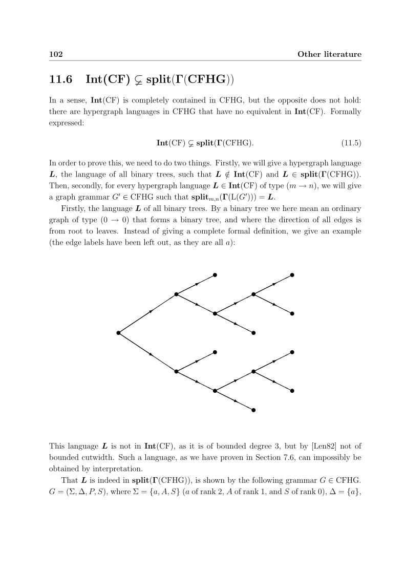
102 Other literature
11.6 Int(CF) split(Γ(CFHG))
In a sense, Int(CF) is completely contained in CFHG, but the opposite does not hold:
there are hypergraph languages in CFHG that have no equivalent in Int(CF). Formally
expressed:
Int(CF) split(Γ(CFHG). (11.5)
In order to prove this, we need to do two things. Firstly, we will give a hypergraph language
L, the language of all binary trees, such that L /∈ Int(CF) and L ∈ split(Γ(CFHG)).
Then, secondly, for every hypergraph language L ∈ Int(CF) of type (m → n), we will give
a graph grammar G′ ∈ CFHG such that splitm,n(Γ(L(G′))) = L.
Firstly, the language L of all binary trees. By a binary tree we here mean an ordinary
graph of type (0 → 0) that forms a binary tree, and where the direction of all edges is
from root to leaves. Instead of giving a complete formal definition, we give an example
(the edge labels have been left out, as they are all a):
u
3
QQQ
QQs
u
*
HHHHHH
HHHHj
u
*
HHHHHH
HHHHj
u
*
HHHHHH
HHHHj
u
u
*
HHHHHH
HHHHj
u
u
u
*
HHHHHH
HHHHj
u
u
*
HHHHHH
HHHHj
u
u
u
u
This language L is not in Int(CF), as it is of bounded degree 3, but by [Len82] not of
bounded cutwidth. Such a language, as we have proven in Section 7.6, can impossibly be
obtained by interpretation.
That L is indeed in split(Γ(CFHG)), is shown by the following grammar G ∈ CFHG.
G = (Σ, ∆, P, S), where Σ = a, A, S (a of rank 2, A of rank 1, and S of rank 0), ∆ = a,

Int(CF) split(Γ(CFHG)) 103
P = π1, π2, π3. The three productions in P look as follows (we mimic the notation of
[EH91]):
S ::= u A1 A ::= u1
*a
HHHHHH
HHHHja
u
u
A1
A1
A ::= u1
Clearly, this G generates all binary trees, or formally, split0,0(Γ(L(G))) = L. Therefore,
L ∈ split(Γ(CFHG)).
Secondly, for a given hypergraph language L ∈ Int(CF) of type (m → n), we will
construct a graph grammar G′ ∈ CFHG such that L(G′) = Γ←(L), so splitm,n(Γ(L(G′))) =
L. This grammar G′ can be constructed as follows8. Let G = (N, T, P, S) be a typed
grammar, and I = (Σ, ∆, h) (where Σ = T ) an interpreter for L(G), such that IntI(L(G)) =
L. Now choose G′ = (Σ′, ∆′, P ′, S ′) as follows:
• Σ′ = N ∪ ∆,
where for a ∈ Σ′, rankΣ′(a) =
#inN(a) + #outN(a) if a ∈ N,
rank∆(a) if a ∈ ∆,
• ∆′ = ∆ (the ranks of its symbols have already been determined above),
• P ′ = πp | p ∈ P .
If p has the form9:
A0 → w1A1w2 . . . wk−1Ak−1wk,
for some k ≥ 1, and for all 1 ≤ i < k, mi = #inN(Ai) and ni = #outN(Ai), then
the production πp looks as follows:
πp = (A0,Γ←(h(w1) · H(A1) · h(w2) · . . . · h(wk−1) · H(Ak−1) · h(wk))),
where:
H(Ai) = (v1, . . . , vmi+ni, e,nod(e) 7→ (v1, . . . , vmi+ni
), lab(e) = Ai,
(v1, . . . , vmi), (vmi+1, . . . , vmi+ni
)) : mi → ni.
Note that this H is type preserving.
8The construction is a more-or-less straightforward extension of the second construction in Section 11.4.9Note the λ-case! (See also the footnote on page 14.)
104 Other literature
• S ′ = S.
We now claim that splitm,n(Γ(L(G′))) = L. Instead of giving a full formal proof, we will
give the invariant that describes the relation between the derivations in G and G′.
Invariant:
For all H ∈ BC-HGR(Σ′), k = |nont(H)| + 1, and j ∈ N:
∃ w1,...,wk∈T ∗
A1,...,Ak−1∈N
G : S ⇒j w1A1w2 . . . wk−1Ak−1wk
and
H = Γ←(h(w1) · H(A1) · h(w2) · . . . · h(wk−1) · H(Ak−1) · h(wk))
⇐⇒
G′ : S ′ ⇒j H.
By the validity of our claim, and because L(G′) ∈ CFHG (by definition), we now have
L ∈ split(Γ(CFHG)). This proves that Int(CF) ⊆ split(Γ(CFHG)). Together with the
first part, this completes the overall proof of Int(CF) split(Γ(CFHG)).
11.7 Bauderon and Courcelle
The hypergraphs defined by Bauderon and Courcelle ([BC87]), are the same BC-hyper-
graphs we mentioned earlier in Section 11.2, except for minor notational differences. The
(single) sequence of external nodes is called the sequence of sources, denoted src, and the
incidence function is called vert (for vertices, i.e., nodes). To translate back and forth
between our hypergraphs and these hypergraphs we will use the same functions Γ and Γ←
we used in Section 11.2.
Bauderon and Courcelle define three kinds of operations on BC-hypergraphs:
• Sum, a binary operation, denoted by H ⊕ H′,
• Redefinition of Sources, a unary operation, denoted by σα(H),
• Source Fusion, a unary operation, denoted by θδ(H).
Loosely speaking, these operations perform the following actions. Let H and H′ be arbi-
trary BC-hypergraphs of rank n and rank n′ respectively. The operation H ⊕ H′ does the
same thing as our parallel composition, but note the fact that it operates on hypergraphs
that have only one sequence of external nodes. The sum H ⊕ H′ has rank n + n′. The
Bauderon and Courcelle 105
operation σα(H), where α is a mapping from [m] to [n] redefines the sequence of n source
nodes of H in a new sequence of m source nodes, in such a way that, for 1 ≤ i ≤ m, the new
source node i is the old source node α(i). So, σα(H) is of rank m. The operation θδ(H),
where δ is an equivalence relation on [n] (intuitively: on the external nodes), identifies
those external nodes srcH(i), srcH(j), 1 ≤ i, j ≤ n, such that (i, j) ∈ δ. So intuitively,
θδ(H) identifies those external nodes of H that are in the relation (as implied by) δ. The
result is again a BC-hypergraph of rank n.
These operations can be expressed in terms of our sequential and parallel composition,
and sequential and parallel composition can be expressed in terms of ⊕, σα, and θδ. in
the following way. Let H and H′ be arbitrary BC-hypergraphs of rank n and rank n′
respectively.
Sum:
The sum H ⊕ H′ can be expressed in terms of + as follows:
Γ(H ⊕ H′) = Γ(H) + Γ(H′).
Redefinition of Sources:
For a mapping α from [m] to [n], σα(H) can be expressed in terms of · as follows:
Γ(σα(H)) = Hα · Γ(H),
where Hα = (v1, . . . , vn,∅,∅,∅, (vα(1), . . . , vα(m)), (v1, . . . , vn)) : m → n.
Source Fusion:
For an equivalence relation δ on [n], θδ(H) can be expressed in terms of · as follows:
Γ(θδ(H)) = Hδ · Γ(H),
where Hδ = ([n]/δ,∅,∅,∅, ([1]δ, . . . , [n]δ), ([1]δ, . . . , [n]δ)) : n → n.
Parallel Composition:
The parallel composition of two hypergraphs H : m → n and H ′ : m′ → n′ can be expressed
in terms of ⊕ and σα as follows:
Γ←(H + H ′) = σα(Γ←(H) ⊕ Γ←(H ′)).

106 Other literature
Here α denotes a mapping from [m + m′ + n + n′] to [m + n + m′ + n′], defined by:
α(i) =
i for 1 ≤ i ≤ m,
i + n for m + 1 ≤ i ≤ m + m′,
i − m′ for m + m′ + 1 ≤ i ≤ m + m′ + n,
i for m + m′ + n + 1 ≤ i ≤ m + m′ + n + n′.
Sequential Composition:
The sequential composition of two hypergraphs H : m → n and H ′ : n → k can be
expressed in terms of σα and θδ as follows:
Γ←(H · H ′) = σα(θδ(Γ←(H) ⊕ Γ←(H ′))).
Here δ denotes the smallest equivalence relation on [m+2n+k] that contains the following
pairs:
(i, j) | m + 1 ≤ i ≤ m + n and j = i + n ,
and α is the mapping from [m + k] to [m + 2n + k] defined by:
α(i) =
i for 1 ≤ i ≤ m,
i + 2n for m + 1 ≤ i ≤ m + k.
Concluding, we have now proved that the operations ⊕, σα, and θδ can be expressed
in terms of · and +, and vice versa. Intuitively, this means that the graph grammars
(or rather expression grammars, where the expressions define graphs) that are defined
by Bauderon and Courcelle in [BC87], could also have been defined using sequential and
parallel composition, in such a way that their power stays exactly the same (it cannot
increase, as the emulation of the operations goes both ways). Neither the formal expression
of this intuition, nor its proof, are trivial. As both are beyond the scope of this thesis, we
will make no attempt at formulating them.
11.8 Habel and Kreowski
In their paper “May we introduce to you: hyperedge replacement” [ENRR87, page 15–26]
Habel and Kreowski make a strong case for taking a hypergraph edge rewriting approach
to graph grammars. The hypergraphs they define look very much like our hypergraphs,
having a sequence of “input” nodes (called begin) and a sequence of “output” nodes (called
end). However, they differ in the fact that the hyperedge-label alphabet is ranked instead
Further reading 107
of typed. Consequently, their hyperedges have two kind a tentacles: source tentacles, and
target tentacles. This makes the hyperedge replacement scheme they propose conceptually
very easy: one “lifts” a hyperedge out of a hypergraph, and then inserts an edge replacing
hypergraph, thereby connecting the begin and end sequences to the former source and
target nodes of the removed edge.
In this respect, their approach looks very much like the approach taken by Bauderon and
Courcelle (and, later, by Engelfriet and Heyker), albeit that Habel and Kreowski choose
to have two sequences of external nodes per hypergraph, and two sequences of tentacles
per hyperedge. As Bauderon and Courcelle correctly point out [BC87, page 113], this does
not increase the power of formalism: both kinds of graph grammars can be emulated by
the other. Therefore, it may be considered a matter of taste whether one wants one or two
sequences of external nodes. In the above mentioned paper Habel and Kreowski argue, by
giving quite a few real-life examples, that having two sequences is preferable.
However, in order to avoid some complications that arise with identification, Habel and
Kreowski do not allow nodes to appear more than once in the begin and end sequences of
a graph. This puts a real restriction on the class of graph languages that can be generated,
albeit not a severe one. Informally speaking, the same languages that could by generated
without this restriction can still be generated, minus the non identification-free graphs they
contained. This was proved by Engelfriet and Heyker in 1992, see [EH92, page 171].
11.9 Further reading
As noted, for an overview of recent developments in the field of graph grammars, [ENRR87]
and [EKR91] are a good place to start, especially because they contain comprehensive
tutorials. Furthermore, the Ph.D. thesis of Habel [Hab92] contains lots of interesting
results. As a matter of fact, at the time of this writing it is the only existing book on
the (modern) theory of context-free graph grammars, and one of the few books at all, and
probably the most up-to-date one, on graph grammars.
Finally, the reader should be well aware of the fact that there is a large area of the
field that has been barely touched upon in this master’s thesis: node replacement graph
grammars. For an introduction to this kind of approach, read the tutorials by Engelfriet
and Rozenberg, [ENRR87, page 55–66] and [EKR91, page 12–23].


There was things which he stretched
but mainly he told the truth.
— Mark Twain 12Summary
This thesis is about the formalism of interpretation. This concept is closely linked to that
of a graph grammar. In Chapter 2 we extended the well-known concepts of grammars and
languages to typed variants of them. We had to do this to be able to exercise strong control
on the types of our objects, in order to ensure they are properly defined. Then we defined
a special kind of graph, the i/o-hypergraph (Chapter 3). On this type of graph, we defined
two main operations: sequential composition and parallel composition (Chapter 4), which
can be used to compose larger graphs from smaller ones. The relation between the two, and
some of their properties were investigated. Then in Chapter 5 we looked at the opposite:
decomposing large graphs into smaller ones. We found a small set of small graphs, called
the full base set, that serve as building blocks to build all other graphs with sequential and
parallel composition.
In Chapter 6, we defined several more operations (of minor importance than composi-
tion) on graphs, and gave some properties. These were mainly needed in proofs of theorems
that do not contain these operations, but still intuitively are based on them. These oper-
ations seem quite natural to us, and their properties have a beauty of their own.
Having defined all the above concepts, we were finally able to introduce the pivot of this
thesis: interpretation (Chapter 7). Interpretation is a mechanism by which we can obtain
a graph language, on the basis of a given string language. As we argued, the formalism
of interpretation may be considered a special kind of an edge-rewriting graph grammar
formalism, albeit in disguise. We gave a few examples of how interpretation works, and
developed a normal form for it. Furthermore, we proved that if a graph language obtained
109

110 Summary
by interpretation has bounded degree, it must also have bounded cutwidth.
Now having completely defined interpretation, in Chapter 8 we turned to the power of
our formalism. We looked at right-linear, linear, and derivation-bounded languages, and
found that all three yield the same class of hypergraph languages under interpretation.
However, the class of all context-free languages under interpretation does give a larger class
of hypergraph languages. We also proved (Section 8.3) that “repeated” interpretation (in
some sense), usually does not increase its power. Finally, we gave two theorems on the
power of interpretation.
The first one gives, given a class K ′ that satisfies some closure properties, the largest
class K such that Int(K) is still contained in Int(K ′). The second one, intuitively, says
that for two classes of string languages K and K ′, if we want to know whether Int(K)
and Int(K ′) are equal, we just have to check some simple closure properties, and prove
the equality for the string graphs in Int(K) and Int(K ′) only.
In Chapter 9, we examined the closure properties of Int(K) in terms of sufficient closure
properties on K, in particular for closure under sequential and parallel composition, union,
Kleene closure, fold, backfold, split, flip, and edge relabeling.
Then, in Chapter 10 we showed that the class of all regular languages under interpre-
tation is identical to the smallest class of hypergraph languages that is closed under both
sequential and parallel composition, union, and Kleene closure, and that contains the full
base set. As a similar characterization is used in traditional formal language theory to
define the class of all regular languages, it can be argued that Int(RLIN) deserves to be
called “the class of all regular hypergraph languages”.
To conclude, in Chapter 11 we looked at a few other formalisms for graph grammars
that have been described in the literature. We made a comparison between some of the
classes of hypergraph languages we defined, and some of those that have been described by
others. In particular we found that Int(RLIN) ≈ LIN-CFHG, which may also be used to
argue that this class deserves to be called “the class of all regular hypergraph languages”.

So long, and thanks for all the fish.
— Douglas Adams 13Acknowledgments
First and foremost, I would like to thank dr. Joost Engelfriet. For the honesty of rejecting
preliminary versions of this thesis time after time, and for the extensive weekly guidance.
For teaching me how to transform my vague intuitions into solid mathematical writing
(did I make progress, or did you give up?), and for more than a year of pleasant Tuesday
afternoon conversations. You have been as good a thesis supervisor as one could wish for,
and I am in your debt for the numerous suggestions and ideas that have finally led to this
thesis.
Then, I would like to thank drs. Gerard Borsboom for teaching me TEX and putting
up with the silly questions. Also thanks to Hans van Dongen for laboriously proofreading
the complete final draft, for laughing himself to tears over a quite erroneous version of
Section 5.6, and for all the beer. Thanks to Huibert Kreb for pointing out the difference
between inherently true propositions, which need no proof, and true theorems, which are
merely true by virtue of their proof, and will loose their validity real soon after that proof
gets lost (see [Kre92]).
Furthermore thanks to ir. Erik Olofsen, ir. Tycho Lamerigts, Carin Tiggeloven, and
Maarten van Dantzich, for their various useful comments, and to dr. Hendrik-Jan Hooge-
boom for showing me how real books number empty pages (they don’t). Thanks to ir. Erik
Kruyt too, for generously providing computer facilities, and to the various people who were
involved in creating the TEX, METAFONT, emTEX, LaTEX, and AMS-LaTEX suites of type-
setting software, all of which were extensively used in creating this document.
This thesis would not have been possible without the help of drs. Frits Vereijken and
111
112 Acknowledgments
Berth Vereijken-Baeten, whom I thank for their continuous moral and financial support
throughout my study.
Last but not least, I am greatly indebted to Tieleke Stibbe, for being my main source of
inspiration, and for trying to understand the difference between hypergraphs, hypergraph
languages, and classes of the latter. It is to you, with love, I dedicate this thesis.
Jan Joris Vereijken,
Leiden, May 19, 1993.
The nice thing about standards is that
there are so many to choose from.
— Andrew S. Tanenbaum ANaming conventions
The names of variables, functions, etc. are called identifiers. In assigning those names we
have strictly adhered to the following conventions.
• Uppercase roman letters:
– For propositions we use a P, or a Q.
• Uppercase italic letters:
– For sets in general we use letters late in the alphabet: V , W .
– For a set that is a string language we use an L. For one that is a class of
languages a K. For a set of terminal symbols: T . For a set of nonterminal
symbols: N . For a set of productions: P or Q. For a set of vertices: V . For a
set of edges: E.
– For the starting symbol in a nonterminal alphabet an S.
– For grammars: G. For a property of grammars: X.
– For hypergraphs we use letters near “H”: H, G, F .
– For interpreters we use an I.
– For nonterminal symbols we use letters early in the alphabet: A, B, C, D.
113
114 Naming conventions
• Lowercase italic letters:
– For integers we use letters near the middle of the alphabet: n, m, k, l, i, j, r,
p, q.
– For terminal symbols we use letters early in the alphabet: a, b, c, d. The a is
also used for a symbol in general.
– For functions in general we use letters near “f”: f , g, h.
– For productions we use letters near “p”: p, q.
– For strings over terminal symbols we use letters near the end of the alphabet:
w, v, u, z.
– For vertices: v, w, u, z. For edges: e.
– For (regular) expressions: r.
• Greek upper case letters:
– For alphabets: Σ, ∆.
• Greek lower case letters:
– For strings over terminal symbols, nonterminal symbols, or both, we use letters
early in the alphabet: α, β, γ, δ.
– For morphisms on string languages: σ.
– For numbers that denote a maximum or minimum in some sense: µ.
• Other cases:
– For ad hoc functions that yield hypergraphs we use bold uppercase italic letters
near “H”: H , G, F .
– For hypergraph languages, and occasionally for sets of hypergraphs, we use a
bold uppercase italic “L”: L. For classes for hypergraph languages: K.
– For EH-hypergraphs and BC-hypergraphs (see Chapter 11) we will use “calli-
graphic” uppercase letters near “H”: H, G, F .
– General functions on hypergraphs are: #in, #out, flip, fold, backfold, split.
– In specific cases we are allowed to abandon the general naming rules, and in-
troduce identifiers of our own choosing. These must however keep their fixed
meaning throughout the whole thesis. The following is a complete list of them:
N, TRUE, FALSE. L, Lτ , G, Gτ , P , Un, λ, RLIN, LIN, DB, CF, rank, nod,
115
lab, in, out, deg, HGR, BC-HGR, Sing, Int, Γ, Γ←, Ωa, 1m,n, Ππ,π′,k, gr,
STR, match.
– When we refer to results from other sources, we may choose to adapt their
notation. See for example Section 11.4, where we use notation from [EH91].
In general our symbols may be subscripted (e.g., A1, ap, αi) at wish if we need more of
them than are available otherwise. The same holds for priming them (e.g., a′, H ′′), or
barring them (e.g., a). We also may build new symbols by grouping old symbols together
in a list (e.g., 〈a, i〉, [A1A2A3]). Although some symbols have more than one use (V , u, v,
w, z, p, q and G), this is not a problem in practice.

Seek simplicity, and distrust it.
— Alfred North Whitehead BProofs
As a rule, proofs are given right after the theorem they prove. However, some theorems are
small, beautiful, and “obviously” true, but have nonetheless long, tedious, and bothersome
proofs. It is this category of proofs that are not given in the main text, but in this appendix.
B.1 Proofs concerning Section 6.3
The six properties from Section 6.3 can be proven by introducing unity hypergraphs U to
the left and the right of all H’s involved, and then “massaging” the H’s out by applying
(4.10) and the basic properties from Section 6.2. As a result, we get the same proper-
ties back again, but now applied to the unity hypergraphs U only. The thus simplified
properties can then be proven directly by expanding the definitions involved.
We will not write out these proof in full however, as they are very long, and worse, they
do not attribute at all to a better understanding of the properties. Instead, we will give
a graphical representation of the structure of the properties. In the following pictures, a
thick line indicates a hypergraph, and a dot indicates external nodes. An arrow in the line
points form in to out to avoid confusion. Folding is indicated folding the line, and flipping
by flipping it (hence the names!). Finally, a thin-lined bounding box is drawn around the
hypergraph that is formed by evaluating the parallel compositions in the properties. First
we give the equation of the property, and then a picture of the structure.
117

118 Proofs
Property (6.32):
fold(H2) · (flip(H1) + H3) = fold(H1H2H3)
Structure:
uu
?H2 ·
u uH1
u u-H3= u
u?H2
u uH1
u u-H3
Property (6.33):
(H1 + flip(H3)) · backfold(H2) = backfold(H1H2H3)
Structure:
u u-H1
u uH3· u
u ?H2 =
u u-H1
u uH3 uu
?H2
Property (6.34):
(H1 + fold(H3)) · (backfold(H2) + H4) = H1H2H3H4
Structure:
u u-H1
uu
?H3
· uu
?H2
u u-H4
=
u u-H1
uu
?H2
uu
?H3 u u-H4
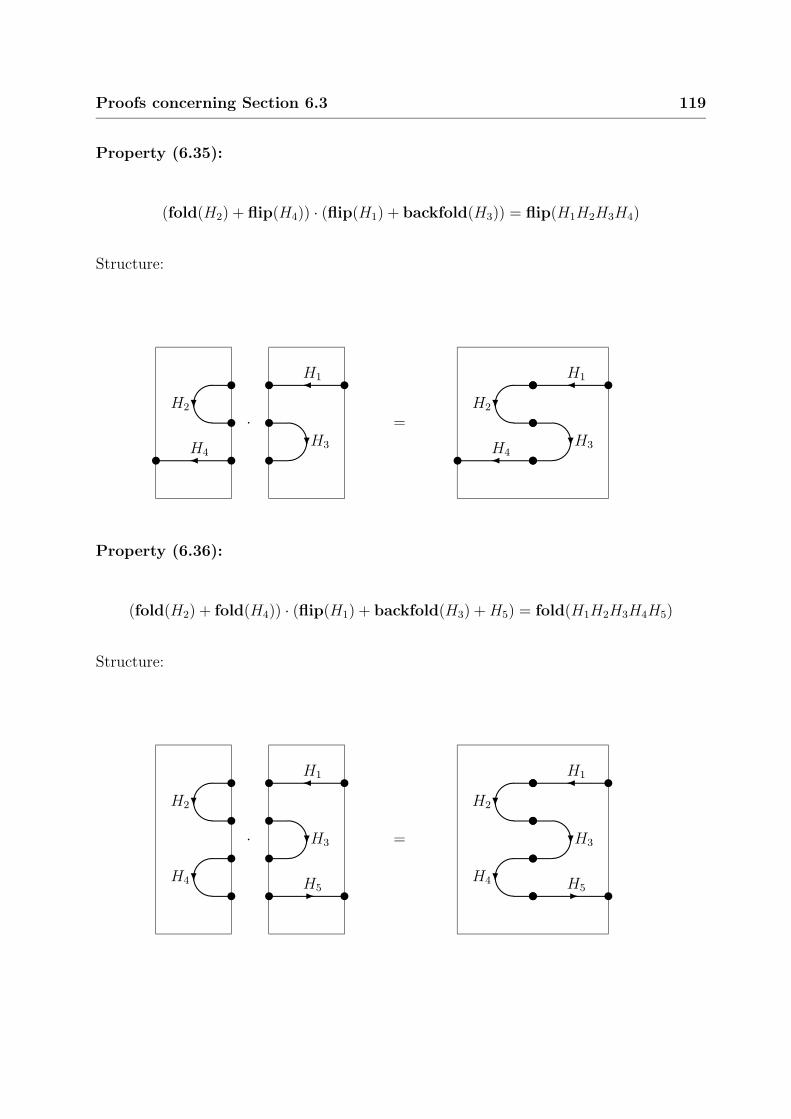
Proofs concerning Section 6.3 119
Property (6.35):
(fold(H2) + flip(H4)) · (flip(H1) + backfold(H3)) = flip(H1H2H3H4)
Structure:
uu
?H2
u uH4
·
u uH1
uu
?H3
=
u uH1
uu
?H2
uu
?H3u uH4
Property (6.36):
(fold(H2) + fold(H4)) · (flip(H1) + backfold(H3) + H5) = fold(H1H2H3H4H5)
Structure:
uu
?H2
uu
?H4
·
u uH1
uu
?H3
u u-H5
=
u uH1
uu
?H2
uu
?H3
uu
?H4 u u-H5
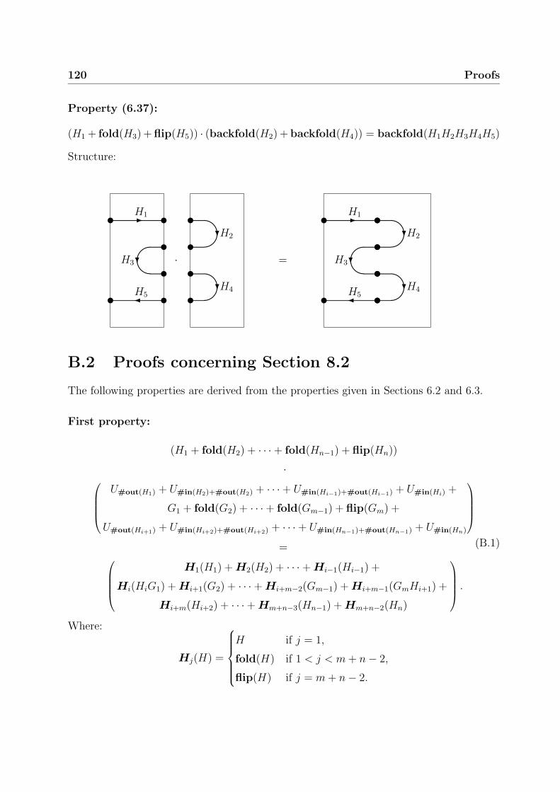
120 Proofs
Property (6.37):
(H1 + fold(H3) + flip(H5)) · (backfold(H2) + backfold(H4)) = backfold(H1H2H3H4H5)
Structure:
u u-H1
uu
?H3
u uH5
·
uu
?H2
uu
?H4
=
u u-H1
uu
?H2
uu
?H3
uu
?H4u uH5
B.2 Proofs concerning Section 8.2
The following properties are derived from the properties given in Sections 6.2 and 6.3.
First property:
(H1 + fold(H2) + · · · + fold(Hn−1) + flip(Hn))
·
U#out(H1) + U#in(H2)+#out(H2) + · · · + U#in(Hi−1)+#out(Hi−1) + U#in(Hi) +
G1 + fold(G2) + · · · + fold(Gm−1) + flip(Gm) +
U#out(Hi+1) + U#in(Hi+2)+#out(Hi+2) + · · · + U#in(Hn−1)+#out(Hn−1) + U#in(Hn)
=
H1(H1) + H2(H2) + · · · + Hi−1(Hi−1) +
Hi(HiG1) + Hi+1(G2) + · · · + Hi+m−2(Gm−1) + Hi+m−1(GmHi+1) +
Hi+m(Hi+2) + · · · + Hm+n−3(Hn−1) + Hm+n−2(Hn)
.
(B.1)
Where:
Hj(H) =
H if j = 1,
fold(H) if 1 < j < m + n − 2,
flip(H) if j = m + n − 2.
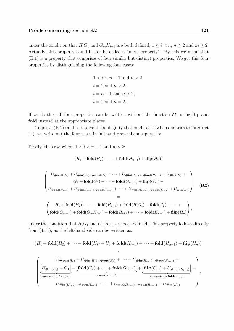
Proofs concerning Section 8.2 121
under the condition that HiG1 and GmHi+1 are both defined, 1 ≤ i < n, n ≥ 2 and m ≥ 2.
Actually, this property could better be called a “meta property”. By this we mean that
(B.1) is a property that comprises of four similar but distinct properties. We get this four
properties by distinguishing the following four cases:
1 < i < n − 1 and n > 2,
i = 1 and n > 2,
i = n − 1 and n > 2,
i = 1 and n = 2.
If we do this, all four properties can be written without the function H , using flip and
fold instead at the appropriate places.
To prove (B.1) (and to resolve the ambiguity that might arise when one tries to interpret
it!), we write out the four cases in full, and prove them separately.
Firstly, the case where 1 < i < n − 1 and n > 2:
(H1 + fold(H2) + · · · + fold(Hn−1) + flip(Hn))
·
U#out(H1) + U#in(H2)+#out(H2) + · · · + U#in(Hi−1)+#out(Hi−1) + U#in(Hi) +
G1 + fold(G2) + · · · + fold(Gm−1) + flip(Gm) +
U#out(Hi+1) + U#in(Hi+2)+#out(Hi+2) + · · · + U#in(Hn−1)+#out(Hn−1) + U#in(Hn)
=
H1 + fold(H2) + · · · + fold(Hi−1) + fold(HiG1) + fold(G2) + · · · +
fold(Gm−1) + fold(GmHi+1) + fold(Hi+2) + · · · + fold(Hn−1) + flip(Hn)
,
(B.2)
under the condition that HiG1 and GmHi+1 are both defined. This property follows directly
from (4.11), as the left-hand side can be written as:
(H1 + fold(H2) + · · · + fold(Hi) + U0 + fold(Hi+1) + · · · + fold(Hn−1) + flip(Hn))
·
U#out(H1) + U#in(H2)+#out(H2) + · · · + U#in(Hi−1)+#out(Hi−1) +[
U#in(Hi) + G1
]
︸ ︷︷ ︸
connects to fold(Hi)
+ [fold(G2) + · · · + fold(Gm−1)]︸ ︷︷ ︸
connects to U0
+[
flip(Gm) + U#out(Hi+1)
]
︸ ︷︷ ︸
connects to fold(Hi+1)
+
U#in(Hi+2)+#out(Hi+2) + · · · + U#in(Hn−1)+#out(Hn−1) + U#in(Hn)
.

122 Proofs
Applying (4.11) now yields the following expression:
H1U#out(H1) + fold(H2)U#in(H2)+#out(H2) + · · ·+ fold(Hi−1)U#in(Hi−1)+#out(Hi−1) +
fold(Hi)[U#in(Hi)+ G1] + U0[fold(G2) + · · ·+ fold(Gm−1)] + fold(Hi+1)[flip(Gm) + U#out(Hi+1)] +
fold(Hi+1)U#in(Hi+1)+#out(Hi+1) + · · ·+ fold(Hn−1)U#in(Hn−1)+#out(Hn−1) + flip(Hn)U#in(Hn)
which easily reduces to
H1 + fold(H2) + · · · + fold(Hi−1) + fold(HiG1) + fold(G2) + · · · +
fold(Gm−1) + fold(GmHi+1) + fold(Hi+2) + · · · + fold(Hn−1) + flip(Hn)
by applying (4.2) and (6.32). This completes the proof of (B.2).
Secondly, the property (B.1) for the case i = 1 and n > 2 looks like this:
(H1 + fold(H2) + · · · + fold(Hn−1) + flip(Hn))
·
G1 + fold(G2) + · · · + fold(Gm−1) + flip(Gm) +
U#out(H2) + U#in(H3)+#out(H3) + · · · + U#in(Hn−1)+#out(Hn−1) + U#in(Hn)
=
H1G1 + fold(G2) + · · · + fold(Gm−1) + fold(GmH2) +
fold(H3) + · · · + fold(Hn−1) + flip(Hn)
,
(B.3)
under the condition that H1G1 and GmH2 are both defined. It is proved in a similar way
as (B.2), using, amongst others, (6.32).
Thirdly, the case i = n − 1 and n > 2 is as follows:
(H1 + fold(H2) + · · · + fold(Hn−1) + flip(Hn))
·
U#out(H1) + U#in(H2)+#out(H2) + · · · + U#in(Hn−2)+#out(Hn−2) + U#in(Hn−1) +
G1 + fold(G2) + · · · + fold(Gm−1) + flip(Gm)
=
H1 + fold(H2) + · · · + fold(Hn−2) +
fold(Hn−1G1) + fold(G2) + · · · + fold(Gm−1) + flip(GmHn)
,
(B.4)
under the condition that Hn−1G1 and GmHn are both defined. This case too is proved in
a way similar as (B.2), using, amongst others, (6.32) and (6.23).
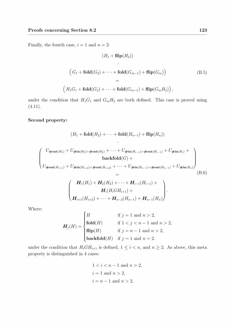
Proofs concerning Section 8.2 123
Finally, the fourth case, i = 1 and n = 2:
(H1 + flip(H2))
·(
G1 + fold(G2) + · · · + fold(Gm−1) + flip(Gm))
=(
H1G1 + fold(G2) + · · · + fold(Gm−1) + flip(GmH2))
,
(B.5)
under the condition that H1G1 and GmH2 are both defined. This case is proved using
(4.11).
Second property:
(H1 + fold(H2) + · · · + fold(Hn−1) + flip(Hn))
·
U#out(H1) + U#in(H2)+#out(H2) + · · · + U#in(Hi−1)+#out(Hi−1) + U#in(Hi) +
backfold(G) +
U#out(Hi+1) + U#in(Hi+2)+#out(Hi+2) + · · · + U#in(Hn−1)+#out(Hn−1) + U#in(Hn)
=
H1(H1) + H2(H2) + · · · + Hi−1(Hi−1) +
Hi(HiGHi+1) +
Hi+1(Hi+2) + · · · + Hn−2(Hn−1) + Hn−1(Hn)
.
(B.6)
Where:
Hj(H) =
H if j = 1 and n > 2,
fold(H) if 1 < j < n − 1 and n > 2,
flip(H) if j = n − 1 and n > 2,
backfold(H) if j = 1 and n = 2.
under the condition that HiGHi+1 is defined, 1 ≤ i < n, and n ≥ 2. As above, this meta
property is distinguished in 4 cases:
1 < i < n − 1 and n > 2,
i = 1 and n > 2,
i = n − 1 and n > 2,
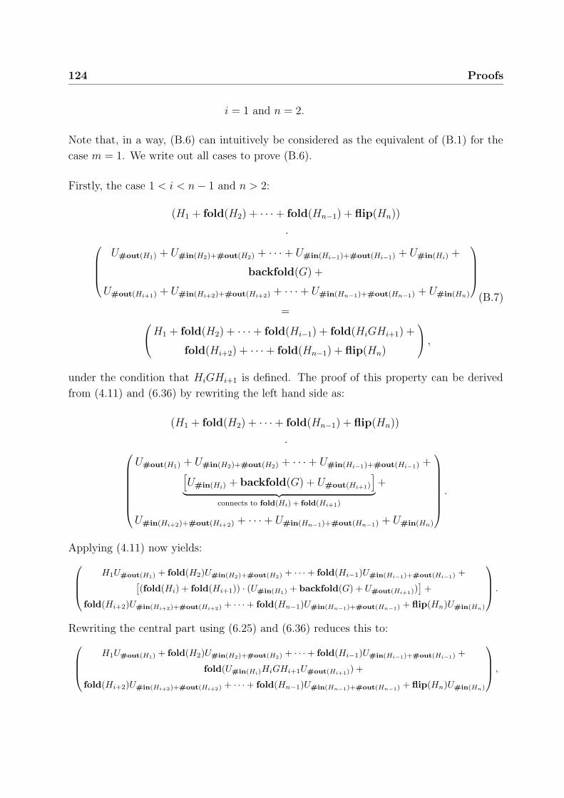
124 Proofs
i = 1 and n = 2.
Note that, in a way, (B.6) can intuitively be considered as the equivalent of (B.1) for the
case m = 1. We write out all cases to prove (B.6).
Firstly, the case 1 < i < n − 1 and n > 2:
(H1 + fold(H2) + · · · + fold(Hn−1) + flip(Hn))
·
U#out(H1) + U#in(H2)+#out(H2) + · · · + U#in(Hi−1)+#out(Hi−1) + U#in(Hi) +
backfold(G) +
U#out(Hi+1) + U#in(Hi+2)+#out(Hi+2) + · · · + U#in(Hn−1)+#out(Hn−1) + U#in(Hn)
=
H1 + fold(H2) + · · · + fold(Hi−1) + fold(HiGHi+1) +
fold(Hi+2) + · · · + fold(Hn−1) + flip(Hn)
,
(B.7)
under the condition that HiGHi+1 is defined. The proof of this property can be derived
from (4.11) and (6.36) by rewriting the left hand side as:
(H1 + fold(H2) + · · · + fold(Hn−1) + flip(Hn))
·
U#out(H1) + U#in(H2)+#out(H2) + · · · + U#in(Hi−1)+#out(Hi−1) +[
U#in(Hi) + backfold(G) + U#out(Hi+1)
]
︸ ︷︷ ︸
connects to fold(Hi) + fold(Hi+1)
+
U#in(Hi+2)+#out(Hi+2) + · · · + U#in(Hn−1)+#out(Hn−1) + U#in(Hn)
.
Applying (4.11) now yields:
H1U#out(H1) + fold(H2)U#in(H2)+#out(H2) + · · · + fold(Hi−1)U#in(Hi−1)+#out(Hi−1) +[(fold(Hi) + fold(Hi+1)) · (U#in(H1) + backfold(G) + U#out(Hi+1))
]+
fold(Hi+2)U#in(Hi+2)+#out(Hi+2) + · · · + fold(Hn−1)U#in(Hn−1)+#out(Hn−1) + flip(Hn)U#in(Hn)
.
Rewriting the central part using (6.25) and (6.36) reduces this to:
H1U#out(H1) + fold(H2)U#in(H2)+#out(H2) + · · · + fold(Hi−1)U#in(Hi−1)+#out(Hi−1) +
fold(U#in(Hi)HiGHi+1U#out(Hi+1)) +
fold(Hi+2)U#in(Hi+2)+#out(Hi+2) + · · · + fold(Hn−1)U#in(Hn−1)+#out(Hn−1) + flip(Hn)U#in(Hn)
,
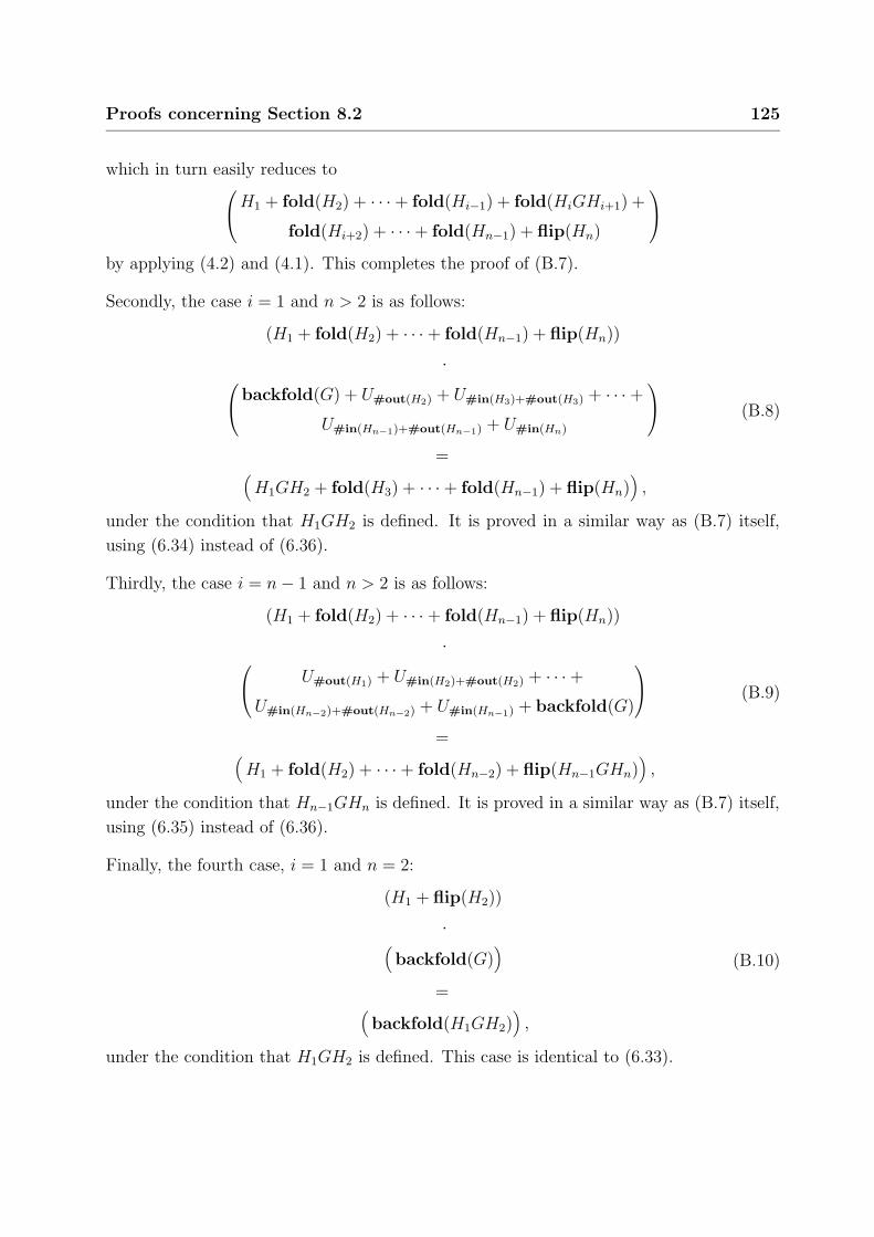
Proofs concerning Section 8.2 125
which in turn easily reduces to
H1 + fold(H2) + · · · + fold(Hi−1) + fold(HiGHi+1) +
fold(Hi+2) + · · · + fold(Hn−1) + flip(Hn)
by applying (4.2) and (4.1). This completes the proof of (B.7).
Secondly, the case i = 1 and n > 2 is as follows:
(H1 + fold(H2) + · · · + fold(Hn−1) + flip(Hn))
·
backfold(G) + U#out(H2) + U#in(H3)+#out(H3) + · · · +
U#in(Hn−1)+#out(Hn−1) + U#in(Hn)
=(
H1GH2 + fold(H3) + · · · + fold(Hn−1) + flip(Hn))
,
(B.8)
under the condition that H1GH2 is defined. It is proved in a similar way as (B.7) itself,
using (6.34) instead of (6.36).
Thirdly, the case i = n − 1 and n > 2 is as follows:
(H1 + fold(H2) + · · · + fold(Hn−1) + flip(Hn))
·
U#out(H1) + U#in(H2)+#out(H2) + · · · +
U#in(Hn−2)+#out(Hn−2) + U#in(Hn−1) + backfold(G)
=(
H1 + fold(H2) + · · · + fold(Hn−2) + flip(Hn−1GHn))
,
(B.9)
under the condition that Hn−1GHn is defined. It is proved in a similar way as (B.7) itself,
using (6.35) instead of (6.36).
Finally, the fourth case, i = 1 and n = 2:
(H1 + flip(H2))
·(
backfold(G))
=(
backfold(H1GH2))
,
(B.10)
under the condition that H1GH2 is defined. This case is identical to (6.33).

Bibliography
[BC87] Michel Bauderon and Bruno Courcelle, Graph expressions and graph rewritings,
Mathematical Systems Theory 20 (1987), no. 2 & 3, 83–127.
[BS87] Mario Benedicty and Frank R. Sledge, Discrete mathematical structures, Har-
court Brace Jovanovich, Orlando, FL, 1987, ISBN 0-15-517683-8.
[CL89] John Carroll and Darrell Long, Theory of finite automata, Prentice-Hall, En-
glewood Cliffs, NJ, 1989, ISBN 0-13-913708-4.
[EH91] Joost Engelfriet and Linda Heyker, The string generating power of context-free
hypergraph grammars, Journal of Computer and System Sciences 43 (1991),
no. 2, 328–360.
[EH92] Joost Engelfriet and Linda Heyker, Context-free hypergraph grammars have
the same term-generating power as attribute grammars, Acta Informatica 29
(1992), 161–210.
[EKR91] H. Ehrig, H.-J. Kreowski, and G. Rozenberg (eds.), Graph grammars and their
application to computer science, Lecture Notes in Computer Science, vol. 532,
Springer-Verlag, Berlin, 1991, 4th International Workshop, Bremen, Germany,
March 1990, ISBN 3-540-54478-X.
[EL89] Joost Engelfriet and George Leih, Linear graph grammars: Power and com-
plexity, Information and Computation 81 (1989), no. 1, 88–121.
[ENRR87] H. Ehrig, M. Nagl, G. Rozenberg, and A. Rosenfeld (eds.), Graph grammars
and their application to computer science, Lecture Notes in Computer Science,
vol. 291, Springer-Verlag, Berlin, 1987, 3rd International Workshop, Warrenton,
Virginia, USA, December 1986, ISBN 3-540-18771-5.
127
128 Bibliography
[ERS80] J. Engelfriet, G. Rozenberg, and G. Slutzki, Tree transducers, L systems, and
two-way machines, Journal of Computer and System Sciences 20 (1980), 150–
202.
[Gre78] S. Greibach, One-way visit automata, Theoretical Computer Science 6 (1978),
175–221.
[Hab92] Annegret Habel, Hyperedge replacement: grammars and languages, Lecture
Notes in Computer Science, vol. 643, Springer-Verlag, Berlin, 1992, ISBN 3-
540-56005-X (originally appeared as Ph.D. thesis, Bremen).
[Her75] I. N. Herstein, Topics in algebra, second ed., John Wiley & Sons, New York,
NY, 1975, ISBN 0-471-02371-X.
[HU79] John E. Hopcroft and Jeffrey D. Ullman, Introduction to automata theory, lan-
guages and computation, Addison-Wesley, Reading, MA, 1979, ISBN 0-201-
02988-X.
[Joh84] Richard Johnsonbaugh, Discrete mathematics, Macmillan Publishing Company,
New York, NY, 1984, ISBN 0-02-360900-1.
[Kam50] E. Kamke, Theory of sets, Dover Publications, New York, NY, 1950, ISBN 0-
486-60141-2 (this is a translation from the German second edition called Menge-
lehre.
[Knu73] Donald Ervin Knuth, Sorting and searching, The Art of Computer Program-
ming, vol. 3, Addison-Wesley, Reading, MA, 1973, ISBN 0-201-03803-X.
[Kre92] Huibert L. Kreb, Proving the klets lemma, Stand-up lecture at Leiden Univer-
sity, unpublished, 1992.
[Len82] T. Lengauer, Upper and lower bounds on the complexity of the min-cut linear
arrangement problem on trees, SIAM Journal of Algebraic Discrete Methods 3
(1982), 99–113.

Index
This index contains references to all definitions and notations used in this thesis. It is not
uncommon for something to be defined more than once. For example, “type” is defined on
page 9 (for a symbol) and on page 18 (for a hypergraph). Furthermore, important concepts
and names of persons have been indexed at the relevant places. Definitions are indicated
by a bold-face number, e.g. 42, and references to naming conventions by a slanted number
e.g. 42.
(∅, m → n), 22
(a, n), 7
(m → n), 9, 10
(v1, . . . , vn), 6
−, 5
=τ , 11
A, 113
B, 113
C, 113
D, 113
E, 113
EH , 17
F , 113
G, 113, 115
G :, 7
H, 113
I, 113
K, 113
L, 113
N , 113
P , 113
Q, 113
S, 113
T , 113
Un, 26, 114
V , 113, 115
V/≡, 6
V ∗, 6
V n, 6
VH , 17
W , 113
X, 113
[(v1, . . . , vn)]≡, 6
[. . . ], 115
[m, n], 5
[n], 5
129

130 Index
[v]≡, 6
#, 6
BC-HGR, 115
BC-HGR(∆), 96
∆, 114
G, 7, 114
Gτ , 12, 114
HGR, 18, 115
HGRm,n(∆), 18
Int, 115
Int(K), 48
Int(L), 48
IntI(L), 48
Int→n(K), 48
Intm→n(K), 48
Intm→(K), 48
L, 7, 114
Lτ , 114
Lτ , 11
N, 5, 114
Ωa, 36, 115
P, 113
Ππ,π′,k, 38, 115
Q, 113
STR, 115
STR(K), 21
Σ, 114
Σ∗, 9
Σ+, 9
Sing, 115
Sing(L), 22
α, 114
≈, 6
Γ, 97, 104, 115
Γ←, 97, 104, 115
1m,n, 37, 115
X, 40
backfold, 43, 114
β, 114
F , 114
G, 114
H , 114
K, 114
L, 114
•, 88
F , 114
G, 114
H, 114
∩, 5
|V |, 6
|α|, 6
·, 7, 25
·m,n,k, 26
, 6
∪, 5
∪m,n, 23·,+−→, 33·
−→, 33
deg, 18, 115
δ, 114
⇒k, 7
⇒∗, 7
∅, 5, 19
≡, 6
≡io, 22
∃, 6
FALSE, 6, 114
flip, 43, 114
fold, 43, 114
∀, 6
γ, 114
gr, 115
gr(w), 21
#in, 18, 114

Index 131
#inΣ, 9
#out, 18, 114
#outΣ, 9
⇐⇒ , 6
=⇒ , 6
∈, 5
lab, 115
labH , 17
λ, 6, 114
∧, 6
〈. . . 〉, 115
∨, 6
7→, 6
match, 115
max, 5
min, 5
µ, 114
3, 5
nod, 114
nodH , 17
in, 115
inH , 17
out, 115
outH , 17
⊕, 104
P , 114
P(V ), 5∏
i, 27
rank, 114
rank(H), 96
rankΣ, 7
L∗, 27
Lk, 27
, 6
\, 5
σ, 114
σα, 104
split, 114
split(K), 45
splitp,q, 43
src, 104
, 5
⊆, 5∑
i, 29
!, 5
⊇, 5
θδ, 104
×, 6
TRUE, 6, 114
vert, 104
a, 114
b, 114
c, 114
d, 114
e, 114
f , 114
f−1, 6
f≡, 6
g, 114
h, 114
i, 114
j, 114
k, 114
l, 114
m, 114
n, 114
p, 114, 115
q, 114, 115
r, 114
u, 114, 115
v, 114, 115
w, 114, 115
wR, 7
z, 114, 115

132 Index
abstract graph, 18
algebra, 41
alphabet, 6
ordinary, 6
ranked, 6
typed, 9
AMS-LaTEX, ii, 111
attack
problems worthy of, iii, 4
backfold
in terms of split, 45
backfolding, 44
closure under, 86
Baeten, Berth, 112
base set
full, 42
sequential, 41
Bauderon, Michel, 96, 104, 106, 107
BC-hypergraph, 96
graph grammar using, 97
binary tree, 56, 102
Borsboom, Gerard, 111
bounded cutwidth, 23, 102
theorem on, 54
bounded degree, 23, 102
theorem on, 54
cardinality, 5
CF, 7, 114
CFHG, 97, 98, 102
Chomsky hierarchy, 2
closure
summary table, 89
under +Un, Un+, 85
under backfolding, 86
under concatenation, 83
under edge relabeling, 88
under flipping, 86
under folding, 86
under Kleene closure, 84
under parallel composition, 86
under sequential composition, 83
under splitting, 88
under union, 84
combinatorics, 41
composition
parallel, 3, 28
relation between sequential and paral-
lel, 29
sequential, 1, 25
concatenation, 10, 27
closure under, 83
concrete graph, 18
context-free grammar, 7
context-free hypergraph grammar, 97
context-free language, 7
correctly internally typed, 9
Courcelle, Bruno, 96, 104, 106, 107
cut, 20
cutwidth, 20
bounded, 23, 102
lemma on, 20
van Dantzich, Maarten, 111
DB, 7, 114
decomposition, 3, 33
full, 33
sequential, 33
definitions
regarding alphabets, 6
regarding classes of languages, 7
regarding functions, 6
regarding grammars, 7
regarding logic, 6
regarding numbers, 5
Index 133
regarding relations, 6
regarding sequences, 6
regarding sets, 5
regarding strings, 7
degree, 18
bounded, 23, 102
vs sequential composition, 27
degree of string graph, 21
Degree versus Cutwidth Theorem, 54
derivation bound, 8
derivation-bounded grammar, 8
derivation-bounded language, 8
disguise
graph grammar in, 2
van Dongen, Hans, 111
edge, see hyperedge
“laying in line”, 20
Edge Normal Form, 51
theorem, 51
edge relabeling
closure under, 88
edge removal, 35
empty hypergraph, 26
empty hypergraph language, 22
emTEX, 111
eNCE graph grammar, 56
ENF, see Edge Normal Form
Engelfriet, Joost, ii, 4, 56, 79, 81, 95, 96,
107, 111
equal modulo i/o, 22
existence of isomorphic copies, 52
external node, 22, 96
flipping, 44
closure under, 86
fold
in terms of split, 45
folding, 44
closure under, 86
full base set, 42
full decomposition, 33
generic class interpretation, 48
generic interpretation, 48
grammar, 7
context-free, 7
derivation-bounded, 8
linear, 7
ordinary, 12
right-linear, 7
typed, 11
underlying, 12
graph
abstract, 18
concrete, 18
ordinary, 20
string, 20
graph grammar, 1
context-free hypergraph . . . , 97
eNCE, 56
in disguise, 2, 96
using BC-hypergraphs, 97
graphical representation, 19
Greibach, S. A., 101
Habel, Annegret, 96, 106, 107
Herstein, I. N., 41
Heyker, Linda, 79, 81, 95, 96, 107
homomorphism
λ-free, 51
Hoogeboom, Hendrik-Jan, 111
hyperedge, 17
hypergraph, 2
abstract, see graph
BC, 96

134 Index
concrete, see graph
degree of, 18
empty, 26
graphical representation of, 19
identification-free, 18
isomorphic, 18
permutation, 38
product, 25
simple, 18
sum, 28
tentacle of, 19
unity, 26
hypergraph language, 22
empty, 22
singleton, 22
union on, 23
i/o
equal modulo, 22
i/o-hypergraph, 17
identification, 25
identification-free, 18
identifier, 6, 113
iff, 6
incidence function, 17, 104
incident, 18
input node, 2, 17
input type, 2, 9, 18
internal node, 22
internally typed, see correctly . . .
interpretation, 48
example of, 49
generic, 48
generic class, 48
limitations of, 53
power of, 80
string graph in terms of, 48
interpretation function, 48
interpreter, 1, 48
Edge Normal Form, 51
for L, 48
isomorphic copies
existence of, 52
Isomorphic Copies Theorem, 52
isomorphic hypergraph, 18
isomorphism, 18, 52
Kleene closure, 10, 27
closure under, 84
Knuth, Donald Ervin, 41
Kreb, Huibert, 111
Kreowski, Hans-Jorg, 96, 106
Kruyt, Erik, 111
labeling function, 17
lambda trick, 14, 58, 65, 99, 100, 103
Lamerigts, Tycho, 111
language
context-free, 7
derivation-bounded, 8
hypergraph, 22
linear, 7
ordinary, 11
right-linear, 7
typed, 10
underlying, 11
language over, 7
late night fortune cookie, 4
LaTEX, 111
layout
linear, 20
Leih, George, 56
lemma on cutwidth, 20
Lengauer, T., 56
LIN, 7, 114
LIN-CFHG, 98
Index 135
linear grammar, 7
linear language, 7
linear layout, 20
loop, 20
in a string graph, 21
vs sequential composition, 27
METAFONT, 111
mixed type, 22
n-sequence, see sequence
naming, 113
node, 17
external, 22, 96
input, 17
internal, 22
output, 17
normal form, see Edge Normal Form
Olofsen, Erik, 111
operator precedence, 31
ordinary alphabet, 6
ordinary grammar, 12
ordinary graph, 20
loop, 20
sequential composition on, 25
ordinary language, 11
ordinary set, 9
ordinary string, 10
ordinary symbol, 9
OUT(2DGSM), 79
OUT(DTWT), 81
output node, 2, 17
output type, 2, 9, 18
parallel composition, 3, 28
associativity of, 28
closure under, 86
commutativity of, 29
relation with sequential composition,
29
stacking railroad cars metaphor, 3
unity element of, 28
pascal, 8
permutation hypergraph, 38
philosophical sidenote, 11
postfix, 7
proper, 7
Power of Interpretation Theorem I, 79
Power of Interpretation Theorem II, 80
power set, 5
precedence of operators, 31
prefix, 7
proper, 7
problems
worthy of attack, iii, 4
product, 25
of ordinary graphs, 25
pseudo base set, see sequential . . .
quotation from
A. N. Onymous, 83
Abraham Lincoln, 1
Alfred North Whitehead, 117
Andrew S. Tanenbaum, 113
Donald Ervin Knuth, 47
Douglas Adams, 111
Edsger Wybe Dijkstra, 5
Harry S. Truman, 91
J. Finnigan, 25
Joost Engelfriet and George Leih, 57
Leonhard Euler, 17
Lewis Carroll, 33
Mark Twain, 109
Phil Collins, 95
The American Heritage Dictionary, 43

136 Index
railroad cars metaphor, 2
rank, 6
ranked alphabet, 6
REG, 7
regular, 7
regular expression, 92
reversal, 7, 87
right-linear grammar, 7
right-linear language, 7
Rijksuniversiteit te Leiden, 4
RLIN, 7, 114
Rosenfeld, A., 95
Rozenberg, Grzegorz, 107
Schneider, H. J., 95
n-sequence, see sequence
sequential composition, 1, 25
associativity of, 26
closure under, 83
commutativity of, 27
hooking railroad cars metaphor, 3
of ordinary graphs, 25
relation with parallel composition, 29
unity element of, 26
vs degree, 27
vs loops, 27
sequential decomposition, 33
sequential pseudo base set, 41
set
cardinality of, 5
ordinary, 9
sequence over a, 6
typed, 9
silly index entry, 136
simple hypergraph, 18
singleton class, 23
singleton hypergraph language, 22
source, 104
split
in terms of (back)fold, 45
split-up, 77
splitting, 44
closure under, 88
Stibbe, Tieleke, 112
STR(Int(RLIN)), 78
strictly over, 7
string, 7
ordinary, 10
typed, 10
string graph, 20
contains no loops, 21
degree of, 21
in term of interpretation, 48
substring, 7
sum, 28
symbol
ordinary, 9
typed, 9
tentacle, 19, 98, 107
TEX, 111
theorem
on bounded cutwidth, 54
on bounded degree, 54
on degree versus cutwidth, 54
on Edge Normal Form, 51
on isomorphic copies, 52
on the power of interpretation, 79
Tiggeloven, Carin, 111
tree
binary, 56, 102
λ-trick, see lambda trick
type, 9, 10, 18
input, 2, 9, 18
mixed, 22
output, 2, 9, 18

Index 137
uniform, 10, 18
type conditions, 8
type preservingness, 8
typed
correctly internally, 9
typed class interpretation, 48
typed grammar, 11
typed language, 10
concatenation, 10
Kleene closure, 10
union, 10
typed set, 9
typed string, 10
typed symbol, 9
typing, 2
example from pascal, 8
example from physics, 8
+Un, Un+
closure under, 85
underlying grammar, 12
underlying language, 11
uniform type, 10, 18
union, 10
closure under, 84
on hypergraph languages, 23
unity element
of parallel composition, 28
of sequential composition, 26
unity hypergraph, 26
variable name clash, 6
Vereijken, Frits, 111
Vereijken, Jan Joris, ii, 112
vertex, see node
wheel, 50
word, see string