graph olap: a multi-dimensional framework for graph data ...xyan/papers/kais09_golap.pdf · graph...

Knowl Inf SystDOI 10.1007/s10115-009-0228-9

REGULAR PAPER

Graph OLAP: a multi-dimensional framework for graphdata analysis

Chen Chen · Xifeng Yan · Feida Zhu · Jiawei Han ·Philip S. Yu

Received: 29 December 2008 / Revised: 5 April 2009 / Accepted: 9 May 2009© The Author(s) 2009. This article is published with open access at Springerlink.com

Abstract Databases and data warehouse systems have been evolving from handlingnormalized spreadsheets stored in relational databases, to managing and analyzing diverseapplication-oriented data with complex interconnecting structures. Responding to this emerg-ing trend, graphs have been growing rapidly and showing their critical importance in manyapplications, such as the analysis of XML, social networks, Web, biological data, multimediadata and spatiotemporal data. Can we extend useful functions of databases and data ware-house systems to handle graph structured data? In particular, OLAP (On-Line AnalyticalProcessing) has been a popular tool for fast and user-friendly multi-dimensional analysis ofdata warehouses. Can we OLAP graphs? Unfortunately, to our best knowledge, there areno OLAP tools available that can interactively view and analyze graph data from differ-ent perspectives and with multiple granularities. In this paper, we argue that it is criticallyimportant to OLAP graph structured data and propose a novel Graph OLAP framework.According to this framework, given a graph dataset with its nodes and edges associatedwith respective attributes, a multi-dimensional model can be built to enable efficient on-line analytical processing so that any portions of the graphs can be generalized/specializeddynamically, offering multiple, versatile views of the data. The contributions of this workare three-fold. First, starting from basic definitions, i.e., what are dimensions and measuresin the Graph OLAP scenario, we develop a conceptual framework for data cubes on graphs.We also look into different semantics of OLAP operations, and classify the framework intotwo major subcases: informational OLAP and topological OLAP. Second, we show how agraph cube can be materialized by calculating a special kind of measure called aggregatedgraph and how to implement it efficiently. This includes both full materialization and partial

C. Chen (B) · F. Zhu · J. HanDepartment of Computer Science, University of Illinois at Urbana-Champaign, Urbana, IL 61801, USAe-mail: [email protected]

X. YanDepartment of Computer Science, University of California at Santa Barbara, Santa Barbara, CA, USA

P. S. YuDepartment of Computer Science, University of Illinois at Chicago, Chicago, IL, USA

123

C. Chen et al.

materialization where constraints are enforced to obtain an iceberg cube. As we can see, due tothe increased structural complexity of data, aggregated graphs that depend on the underlying“network” properties of the graph dataset are much harder to compute than their traditionalOLAP counterparts. Third, to provide more flexible, interesting and informative OLAP ofgraphs, we further propose a discovery-driven multi-dimensional analysis model to ensurethat OLAP is performed in an intelligent manner, guided by expert rules and knowledgediscovery processes. We outline such a framework and discuss some challenging researchissues for discovery-driven Graph OLAP.

Keywords Multi-dimensional model · Graph OLAP · Efficient computation · Discovery-driven analysis

1 Introduction

OLAP (On-Line Analytical Processing) [2,7,11,12,31] is an important notion in data anal-ysis. Given the underlying data, a cube can be constructed to provide a multi-dimensionaland multi-level view, which allows for effective analysis of the data from different per-spectives and with multiple granularities. The key operations in an OLAP framework areslice/dice and roll-up/drill-down, with slice/dice focusing on a particular aspect of the data,roll-up performing generalization if users only want to see a concise overview, and drill-downperforming specialization if more details are needed.

In a traditional data cube, a data record is associated with a set of dimensional values,whereas different records are viewed as mutually independent. Multiple records can be sum-marized by the definition of corresponding aggregate measures such as COUNT, SUM,and AVERAGE. Moreover, if a concept hierarchy is associated with each attribute, multi-level summaries can also be achieved. Users can navigate through different dimensions andmultiple hierarchies via roll-up, drill-down and slice/dice operations. However, in recentyears, more and more data sources beyond conventional spreadsheets have come into being,such as chemical compounds or protein networks (chem/bio-informatics), 2D/3D objects(pattern recognition), circuits (computer-aided design), XML (data with loose schemas) andWeb (human/computer networks), where not only individual entities but also the interactingrelationships among them are important and interesting. This demands a new generation oftools that can manage and analyze such data.

Given their great expressive power, graphs have been widely used for modeling a lotof datasets that contain structure information. With the tremendous amount of graph dataaccumulated in all above applications, the same need to deploy analysis from different per-spectives and with multiple granularities exists. To this extent, our main task in this paper isto develop a Graph OLAP framework, which presents a multi-dimensional and multi-levelview over graphs.

In order to illustrate what we mean by “Graph OLAP” and how the OLAP glossary isinterpreted with regard to this new scenario, let us start from a few examples.

Example 1 (Collaboration patterns) There are a set of authors working in a given field: Forany two persons, if they coauthor w papers in a conference, e.g., SIGMOD 2004, then alink is added between them, which has a collaboration frequency attribute that is weightedas w. For every conference in every year, we may have a coauthor network describing thecollaboration patterns among researchers, each of them can be viewed as a snapshot of theoverall coauthor network in a bigger context.

123

Graph OLAP: a multi-dimensional framework for graph data analysis

It is interesting to analyze the aforementioned graph dataset in an OLAP manner. First,one may want to check the collaboration patterns for a group of conferences, say, all DBconferences in 2004 (including SIGMOD, VLDB, ICDE, etc.) or all SIGMOD conferencessince the year it was introduced. In the language of data cube, with a venue dimension and atime dimension, one may choose to obtain the (db-conf, 2004) cell and the (sigmod, all-years)cell, where the venue and time dimensions have been generalized to db-conf and all-years,respectively. Second, for the subset of snapshots within each cell, one can summarize themby computing a measure as we did in traditional OLAP. In the graph context, this gives riseto an aggregated graph. For example, a summary network displaying total collaboration fre-quencies can be achieved by overlaying all snapshots together and summing up the respectiveedge weights, so that each link now indicates two persons’ collaboration activities in the DBconferences of 2004 or during the whole history of SIGMOD.

The above example is simple because the measure is calculated by a simple sum overindividual pieces of information. A more complex case is presented next.

Example 2 (Maximum flow) Consider a set of cities connected by transportation networks.In general, there are many ways to go from one city A to another city B, e.g., by bus, bytrain, by air, by water., etc., and each is operated by multiple companies. For example, wecan assume that the capacity of company x’s air service from A to B is cx

AB , i.e., companyx can transport at most cx

AB units of cargo from A to B using the planes it owns. Finally, weget a snapshot of capacity network for every transportation means of every company.

Now, consider the transporting capability from a source city S to a destination city T , it isinteresting to see how this value can be achieved by sending flows of cargo through differentpaths if (1) we only want to go by air, or (2) we only want to choose services operated bycompany x . In the OLAP language, with a transportation-type dimension and a companydimension, the above situations correspond to the (air, all-companies) cell and the (all-types,company x) cell, while the measure computed for a cell c is a graph displaying how themaximum flow can be configured, which has considered all transportation means and oper-ating companies associated with c. Unlike Example 1, computing the aggregated graph ofmaximum flow is now a much harder task; also, the semantics associated with un-aggregatednetwork snapshots and aggregated graphs are different: The former shows capacities on itsedges, whereas the latter shows transmitted flows, which by definition must be smaller.

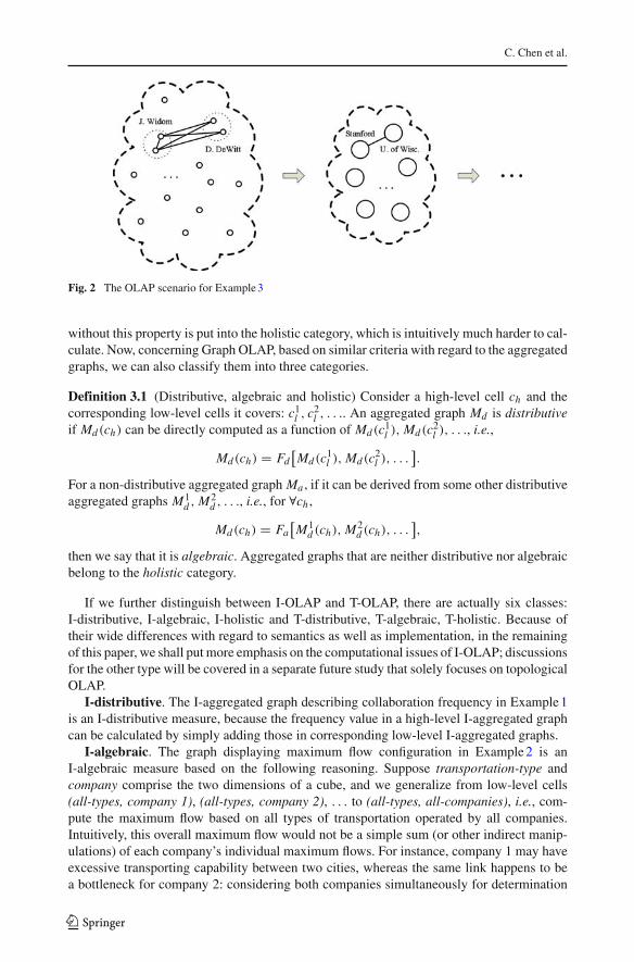
Example 3 (Collaboration patterns, revisited) Usually, the whole coauthor network could betoo big for the users to comprehend, and thus it is desirable to look at a more compressedview. For example, one may like to see the collaboration activities organized by the authors’associated affiliations, which requires the network to be generalized one step up, i.e., merg-ing all persons in the same institution as one node and constructing a new summary graph atthe institution level. In this “generalized network”, for example, an edge between Stanfordand University of Wisconsin will aggregate all collaboration frequencies incurred betweenStanford authors and Wisconsin authors. Similar to Examples 1 and 2, an aggregated graph(i.e., the generalized network defined above) is taken as the OLAP measure. However, thedifference here is that a roll-up from the individual level to the institution level is achievedby consolidating multiple nodes into one, which shrinks the original network. Comparedto this, the graph in Examples 1 and 2 is not collapsed because we are always examiningthe relationships among the same set of objects—it poses minimum changes with regard tonetwork topology upon generalization.

The above examples demonstrate that OLAP provides a powerful primitive to analyzegraph datasets. In this paper, we will give a systematic study on Graph OLAP, which is

123

C. Chen et al.

more general than the traditional OLAP: in addition to individual entities, the mutual inter-actions among them are also considered in the analytical process. Our major contributionsare summarized in below.

1. On conceptual modeling, a Graph OLAP framework is developed, which defines dimen-sions and measures in the graph context, as well as the concept of multi-dimensional andmulti-level analysis over graph structured data. We distinguish different semantics ofOLAP operations and categorize them into two major subcases: informational OLAP (asshown in Examples 1 and 2) and topological OLAP (as shown in Example 3). It is nec-essary since these two kinds of OLAP demonstrate substantial differences with regardto the construction of a graph cube.

2. On efficient implementation, the computation of aggregated graphs as Graph OLAPmeasures is examined. Due to the increased structural complexity of data, calculating cer-tain measures that are closely tied with the graph properties of a network, e.g., maximumflow, centrality, etc., poses greater challenges than their traditional OLAP counterparts,such as COUNT, SUM and AVERAGE. We investigate this issue, categorize measuresbased on the difficulty to compute them in the OLAP context and suggest a few measureproperties that might help further optimize processings. Both full materialization andpartial materialization (where constraints are enforced to obtain an iceberg cube) arediscussed.

3. On utilizing the framework for knowledge discovery, we propose discovery-drivenGraph OLAP, so that interesting patterns and knowledge can be effectively discovered.After presenting the general ideas, we outline a list of guiding principles and discusssome associated research problems. Being part of an ongoing project, it opens a prom-ising path that could lead to more flexible and insightful OLAP of graph data, which weshall explore further in future works.

The remaining of this paper is organized as follows. In Sect. 2, we formally introducethe Graph OLAP framework. Section 3 discusses the general hardness to compute aggre-gated graphs as Graph OLAP measures, which categorizes them into three classes. Section 4looks into some properties of the measures and proposes a few computational optimiza-tions. Constraints and partial materialization are studied in Sect. 5. Discovery-driven GraphOLAP is covered in Sect. 6. We report experiment results and related work in Sects. 7 and8, respectively. Section 9 concludes this study.

2 A Graph OLAP framework

In this section, we present the general framework of Graph OLAP.

Definition 2.1 (Graph model) We model the data examined by Graph OLAP as a collectionof network snapshots G = {G1, G2, . . . , GN }, where each snapshot Gi = (I1,i , I2,i , . . . , Ik,i ;Gi ) in which I1,i , I2,i , . . . , Ik,i are k informational attributes describing the snapshot as awhole and Gi = (Vi , Ei ) is a graph. There are also node attributes attached with any v ∈ Vi

and edge attributes attached with any e ∈ Ei . Note that, since G1, G2, . . . , GN only representdifferent observations, V1, V2, . . . , VN actually correspond to the same set of objects in realapplications.

For instance, with regard to the coauthor network described in the introduction, venueand time are two informational attributes that mark the status of individual snapshots, e.g.,

123


SIGMOD 2004 and ICDE 2005, authorID is a node attribute indicating the identification ofeach node, and collaboration frequency is an edge attribute reflecting the connection strengthof each edge.

Dimension and measure are two concepts that lay the foundation of OLAP and cubes. Astheir names imply, first, dimensions are used to construct a cuboid lattice and partition thedata into different cells, which act as the basis for multi-dimensional and multi-level analysis;second, measures are calculated to aggregate the data covered, which deliver a summarizedview of it. In below, we are going to formally re-define these two concepts concerning theGraph OLAP scenario.

Let us examine dimensions at first. Actually, there are two types of dimensions in GraphOLAP. The first one, as exemplified by Example 1, utilizes informational attributes attachedat the whole snapshot level. Suppose the following concept hierarchies are associated withvenue and time:

• venue: conference → area → all,• time: year → decade → all;

the role of these two dimensions is to organize snapshots into groups based on differentperspectives, e.g., (db-conf, 2004) and (sigmod, all-years), where each of these groups cor-responds to a “cell” in the OLAP terminology. They control what snapshots are to be lookedat, without touching the inside of any single snapshot.

Definition 2.2 (Informational dimensions) With regard to the graph model presented inDefinition 2.1, the set of informational attributes {I1, I2, . . . , Ik} are called the informationaldimensions of Graph OLAP, or Info-Dims in short.

The second type of dimensions are provided to operate on nodes and edges within indi-vidual networks. Take Example 3 for instance, suppose the following concept hierarchy

• authorID: individual → institution → all

is associated with the node attribute authorID, then it can be used to group authors from thesame institution into a “generalized” node, and a new graph thus formed will depict inter-actions among these groups as a whole, which summarizes the original network and hidesspecific details.

Definition 2.3 (Topological dimensions) The set of dimensions coming from the attributesof topological elements (i.e., nodes and edges of Gi ), {T1, T2, . . . , Tl}, are called the topo-logical dimensions of Graph OLAP, or Topo-Dims in short.

The OLAP semantics accomplished through Info-Dims and Topo-Dims are rather differ-ent, and in the following we shall refer to them as informational OLAP (abbr. I-OLAP) andtopological OLAP (abbr. T-OLAP), respectively.

For roll-up in I-OLAP, the characterizing feature is that, snapshots are just differentobservations of the same underlying network, and thus when they are all grouped into onecell in the cube, it is like overlaying multiple pieces of information, without changing theobjects whose interactions are being looked at.

For roll-up in T-OLAP, we are no longer grouping snapshots, and the reorganizationswitches to happen inside individual networks. Here, merging is performed internally which“zooms out” the user’s focus to a “generalized” set of objects, and a new graph formed bysuch shrinking might greatly alter the original network’s topological structure.

Now we move on to measures. Remember that, in traditional OLAP, a measure is calcu-lated by aggregating all the data tuples whose dimensions are of the same values (based on

123

C. Chen et al.

concept hierarchies, such values could range from the finest un-generalized ones to “all/*”,which form a multi-level cuboid lattice); casting this to our scenario here:

First, in Graph OLAP, the aggregation of graphs should also take the form of a graph, i.e.,an aggregated graph. In this sense, graph can be viewed as a special existence, which playsa dual role: as a data source and as an aggregated measure. Of course, other measures thatare not graphs, such as node count, average degree, diameter, etc., can also be calculated;however, we do not explicitly include such non-graph measures in our model, but insteadtreat them as derived from corresponding graph measures.

Second, due to the different semantics of I-OLAP and T-OLAP, aggregating data withidentical Info-Dim values groups information among the snapshots, whereas aggregatingdata with identical Topo-Dim values groups topological elements inside individual networks.As a result, we will give a separate measure definition for each case in below.

Definition 2.4 (I-aggregated graph) With regard to Info-Dims {I1, I2, . . . , Ik}, theI-aggregated graph M I is an attributed graph that can be computed based on a set ofnetwork snapshots G′ = {Gi1 , Gi2 , . . . , GiN ′ } whose Info-Dims are of identical values; itsatisfies: (1) the nodes of M I are as same as any snapshot in G′, and (2) the node/edgeattributes attached to M I are calculated as aggregate functions of the node/edge attributesattached to Gi1 , Gi2 , . . . , GiN ′ .

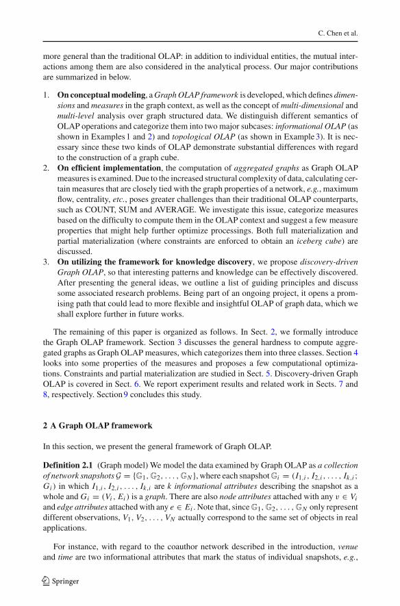
The graph in Fig. 1 that describes collaboration frequencies among individual authorsfor a particular group of conferences during a particular period of time is an instance ofI-aggregated graph, and the interpretation of classic OLAP operations with regard to graphI-OLAP is summarized as follows:

• Roll-up: Overlay multiple snapshots to form a higher-level summary via I-aggregatedgraph.

• Drill-down: Return to the set of lower-level snapshots from the higher-level overlaid(aggregated) graph.

• Slice/dice: Select a subset of qualifying snapshots based on Info-Dims.

Definition 2.5 (T-aggregated graph) With regard to Topo-Dims {T1, T2 . . . , Tl}, theT-aggregated graph MT is an attributed graph that can be computed based on an individualnetwork Gi ; it satisfies: (1) the nodes in Gi that have identical values on their Topo-Dimsare grouped, whereas each group corresponds to a node of MT , (2) the attributes attached toMT are calculated as aggregate functions of the attributes attached to Gi .

The graph in Fig. 2 that describes collaboration frequencies among institutions is aninstance of T-aggregated graph, and the interpretation of classic OLAP operations with regardto graph T-OLAP is summarized as follows.

• Roll-up: Shrink the network topology and obtain a T-aggregated graph that displays com-pressed views. Topological elements (i.e., nodes and/or edges) are merged and replacedby corresponding higher-level ones during the process.

• Drill-down: A reverse operation of roll-up.• Slice/dice: Select a subgraph of the network based on Topo-Dims.

3 Measure classification

Now, with a clear concept of dimension, measure and possible OLAP operations, we areready to discuss implementation issues, i.e., how to compute the aggregated graph in a multi-dimensional and multi-level way.

123


Fig. 1 The OLAP scenario for Example 1

Recall that in traditional OLAP, measures can be classified into distributive, algebraic andholistic, depending on whether the measures of high-level cells can be easily computed fromtheir low-level counterparts, without accessing base tuples residing at the finest level. Forinstance, in the classic sale(time, location) example, the total sale of [2008, California] canbe calculated by adding up the total sales of [January 2008, California], [February 2008,California], . . ., [December 2008, California], without looking at base data points such as[04/12/2008, Los Angeles], which means that SUM is a distributive measure. Compared tothis, AVG has been used to illustrate algebraic measures, which is actually a semi-distributivecategory in that AVG can be derived from two distributive measures: SUM and COUNT, i.e.,algebraic measures are functions of distributive measures.

(Semi-)distributiveness is a nice property for top-down cube computation, where thecuboid lattice can be gradually filled up by making level-by-level aggregations. Measures

123

C. Chen et al.

Fig. 2 The OLAP scenario for Example 3

without this property is put into the holistic category, which is intuitively much harder to cal-culate. Now, concerning Graph OLAP, based on similar criteria with regard to the aggregatedgraphs, we can also classify them into three categories.

Definition 3.1 (Distributive, algebraic and holistic) Consider a high-level cell ch and thecorresponding low-level cells it covers: c1

l , c2l , . . .. An aggregated graph Md is distributive

if Md(ch) can be directly computed as a function of Md(c1l ), Md(c2

l ), . . ., i.e.,

Md(ch) = Fd[Md(c1

l ), Md(c2l ), . . .

].

For a non-distributive aggregated graph Ma , if it can be derived from some other distributiveaggregated graphs M1

d , M2d , . . ., i.e., for ∀ch ,

Md(ch) = Fa[M1

d (ch), M2d (ch), . . .

],

then we say that it is algebraic. Aggregated graphs that are neither distributive nor algebraicbelong to the holistic category.

If we further distinguish between I-OLAP and T-OLAP, there are actually six classes:I-distributive, I-algebraic, I-holistic and T-distributive, T-algebraic, T-holistic. Because oftheir wide differences with regard to semantics as well as implementation, in the remainingof this paper, we shall put more emphasis on the computational issues of I-OLAP; discussionsfor the other type will be covered in a separate future study that solely focuses on topologicalOLAP.

I-distributive. The I-aggregated graph describing collaboration frequency in Example 1is an I-distributive measure, because the frequency value in a high-level I-aggregated graphcan be calculated by simply adding those in corresponding low-level I-aggregated graphs.

I-algebraic. The graph displaying maximum flow configuration in Example 2 is anI-algebraic measure based on the following reasoning. Suppose transportation-type andcompany comprise the two dimensions of a cube, and we generalize from low-level cells(all-types, company 1), (all-types, company 2), . . . to (all-types, all-companies), i.e., com-pute the maximum flow based on all types of transportation operated by all companies.Intuitively, this overall maximum flow would not be a simple sum (or other indirect manip-ulations) of each company’s individual maximum flows. For instance, company 1 may haveexcessive transporting capability between two cities, whereas the same link happens to bea bottleneck for company 2: considering both companies simultaneously for determination

123


of the maximum flow can enable capacity sharing and thus create a double-win situation. Inthis sense, maximum flow is not distributive by definition. However, as an obvious fact,maximum flow f is decided by the network c that shows link capacities on its edges,and this capacity graph is distributive because it can be directly added upon generaliza-tion: When link sharing is enabled, two separated links from A to B, which are operatedby different companies and have capacities c1

AB and c2AB , respectively, are no different

from a single link with capacity c1AB + c2

AB , considering their contributions to the flowvalue. Finally, being a function of distributive aggregated graphs, maximum flow is alge-braic.

I-holistic. The I-holistic case involves a more complex aggregate graph, where base-leveldetails are required to compute it. In the coauthor network of Example 1, the median ofresearchers’ collaboration frequency for all DB conferences from 1990 to 1999 is holistic,similar to what we saw in a traditional data cube.

4 Optimizations

Being (semi-)distributive or holistic tells us whether the aggregated graph computation needsto start from completely un-aggregated data or some intermediate results can be leveraged.However, even if the aggregated graph is distributive or algebraic, and thus we can calculatehigh-level measures based on some intermediate-level ones, it is far from enough, becausethe complexity to compute the two functions Fd and Fa in Definition 3.1 is another ques-tion. Think about the maximum flow example we just mentioned, Fa takes the distributivecapacity graph as input to compute the flow configuration, which is by no means an easytransformation.

Based on our analysis, there are mainly two reasons for such potential difficulties. First,due to the interconnecting nature of graphs, the computation of many graph properties is“global” as it requires us to take the whole network into consideration. In order to make thisconcept of globalness clear, let us first look at a “local” situation: For I-OLAP, aggregatedgraphs are built for the same set of objects as the underlying network snapshots; now, in theaggregated graph of Example 1, “R. Agrawal” and “R. Srikant”’s collaboration frequency forcell (db-conf, 2004) is locally determined by “R. Agrawal” and “R. Srikant”’s collaborationfrequency for each of the DB conferences held in 2004; it does not need any informationfrom the other authors to fulfill the computation. This is an ideal scenario, because the calcu-lations can be localized and thus greatly simplified. Unfortunately, not all measures providesuch local properties. For instance, in order to calculate a maximum flow from S to T forthe cell (air, all-companies) in Example 2, only knowing the transporting capability of eachcompany’s direct flights between S and T is not enough, because we can always take anindirect route via some other cities to reach the destination.

Second, the purpose for us to compute high-level aggregated graphs based on low-levelones is to reuse the intermediate calculations that are already performed. However, whencomputing the aggregated graph of a low-level cell ci

l , we only had a partial view about theci

l -portion of network snapshots; now, as multiple pieces of information are overlaid into thehigh-level cell ch , some full-scale consolidation needs to be performed, which is very muchlike the merge sort procedure, where partial ranked lists are reused but somehow adjustedto form a full ranked list. Still, because of the structural complexity, it is not an easy taskto develop such reuse schemes for graphs, and even it is possible, reasonably complicatedoperations might be involved.

123

C. Chen et al.

Admitting the difficulties in above, let us now investigate the possibility to alleviate them.As we have seen, for some aggregated graphs, the first aspect can be helped by their locali-zation properties with regard to network topology. Concerning the second aspect, the key ishow to effectively reuse partial results computed for intermediate cells so that the workloadto obtain a full-scale measure is attenuated as much as possible. In the following, we aregoing to examine these two directions in sequel.

4.1 Localization

Definition 4.1 (Localization) For an I-aggregated graph Ml that summarizes a group of net-work snapshots G′ = {Gi1 , Gi2 , . . . , GiN ′ }, if 1) we only need to check a neighborhood of v

in Gi1 , Gi2 , . . . , GiN ′ to calculate v’s node attributes in Ml , and 2) we only need to check aneighborhood of u, v in Gi1 , Gi2 , . . . , GiN ′ to calculate (u, v)’s edge attributes in Ml , thenthe computation of Ml is said to be localizable.

Example 4 (Common friends) With regard to the coauthor network depicted in Example 1,we can also compute the following aggregated graph: given two authors a1 and a2, the edgebetween them records the number of their common “friends”, whereas in order to build such“friendship”, the total collaboration frequency between two researchers must surpass a δc

threshold for the specified conferences and time.

The above example provides another instance that leverages localization to promote effi-cient processing. Consider a cell, e.g., (db-conf, 2004), the determination of the aggregatedgraph’s a1-a2 edge can be restricted to a 1-neighborhood of these two authors in the un-aggregated snapshots of 2004’s DB conferences, i.e., we only need to check edges that aredirectly adjacent to either a1 or a2, and in this way a third person a3 can be found, if he/shepublishes with both a1 and a2, while the total collaboration frequency summed from theweights of these adjacent edges is at least δc. Also, note that, the above aggregated graph def-inition is based on the number of length-2 paths like a1-a3-a2 where each edge of it representsa “friendship” relation; now, if we further allow the path length to be at most k, computationscan still be localized in a � k

2�-neighborhood of both authors, i.e., any relevant author on suchpaths of “friendship” must be reachable from either a1 or a2 within � k

2� steps. This can beseen as a situation that sits in the middle of Example 1’s “absolute locality” (0-neighborhood)and maximum flow’s “absolute globality” (∞-neighborhood).

There is an interesting note we want to put for the absolutely local distributive aggregatedgraph of Example 1. Actually, such a 0-neighborhood localization property degenerates thescenario to a very special case, where it is no longer necessary to assume the underlyingdata as a graph: for each pair of coauthors, we can construct a traditional cube showing theircollaboration frequency “OLAPed” with regard to venue and time, whose computation doesnot depend on anything else in the coauthor network. In this sense, we can treat the coauthornetwork as a union of pairwise collaboration activities, whereas Example 1 can indeed bethought as a traditional OLAP scenario disguised under its graph appearances, because thegraph cube we defined is nothing different from a collection of pair-wise traditional cubes.As a desirable side effect, this enables us to leverage specialized technologies that are devel-oped for traditional OLAP, which in general could be more efficient. Nevertheless, the case isspecial, anyway: Absolute localization would not hold for most information network, whichis also the reason why traditional OLAP proves to be extremely restricted when handlingnetworked data.

123


4.2 Attenuation

In below, we are going to explain the idea of attenuation through examples, and the case wepick is maximum flow. In a word, the more partial results from intermediate calculations areutilized, the more we can decrease the cost of obtaining a full-scale aggregated graph.

To begin with, let us first review some basic concepts, cf. [8]. Given a directed graphG = (V, E), c : (V

2

) → R≥0 indicates a capacity for all pairs of vertices and E is pre-cisely the set of vertex pairs for which c > 0. For a source node s and a destination nodet , a flow in G is a function f : (V

2

) → R assigning values to graph edges such that, (i)f (u, v) = − f (v, u): skew symmetry, (ii) f (u, v) ≤ c(u, v): capacity constraint, and (iii)for each v = s/t,

∑u∈V f (u, v) = 0: flow conservation. Since most maximum flow algo-

rithms work incrementally, there is an important lemma as follows.

Lemma 4.1 Let f be a flow in G and let G f be its residual graph, where residual meansthat the capacity function of G f is c f = c − f ; now, f ′ is a maximum flow in G f if andonly if f + f ′ is a maximum flow in G.

Note that, the +/− notation here means edge-by-edge addition/subtraction; and in sum-mary, this lemma’s core idea is to look for a flow f ′ in G f and use f ′ to augment the currentflow f in G.

For the Graph OLAP context we consider, in order to compute the algebraic aggregatedgraph displaying maximum flow, the function Fa takes a distributive capacity graph c as itsinput; now, since capacity can be written as the sum of a flow and a residual graph: c = f +c f ,does this decomposition provide us some hints to pull out the useful part f , instead of blindlytaking c and starting from scratch?

Suppose that the capacity graph of cell (all-types, company 1) is c1, where f1 is themaximum flow and c1

f1= c1 − f1 denotes the corresponding residual graph. Likewise, we

have c2, f2 and c2f2

for cell (all-types, company 2). Without loss of generality, assume thereare only these two companies whose transportation networks are overlaid into (all-types,all-companies), which has a capacity of c = c1 + c2.

Claim 4.1 f1 + f2 + f ′ is a maximum flow for c if and only if f ′ is a maximum flow forc1

f1+ c2

f2.

Proof Since f1 and f2 are restricted to the transportation networks of company 1 and com-pany 2, respectively, the overall capacity c = c1 + c2 must accommodate f1 + f2, even iflink sharing is not enabled. As a result of subtracting f1 + f2, the residual graph becomes:

c f1+ f2 = (c1 + c2) − ( f 1 + f 2)

= (c1 − f 1) + (c2 − f 2) = c1f1

+ c2f2.

A direct application of Lemma 1 finishes our proof.

As it is generally hard to localize maximum flow computations with regard to networktopology, the above property is important because it takes another route, which reuses partialresults f1, f2 and attenuates the overall workload from c1 + c2 to c1

f1+ c2

f2. By doing this,

we are much closer to the overall maximum flow f1 + f2 + f ′ because a big portion of it,f1 + f2, has already been decided even before we start an augmenting algorithm.

However, we should admit that attenuation schemes usually take widely different forms,which might need to be developed with regard to specific aggregate measure graphs; fur-thermore, as we shall see next, there do exist cases where such properties are hard, if notimpossible, to think of.

123

C. Chen et al.

Example 5 (Centrality) Centrality is an important concept in social network analysis, whichreflects how “central” a particular node’s position is in a given network. One definition calledbetweenness centrality CB uses shortest path to model this: Let n jk denote the number ofshortest paths (as there could be equally short ones) between two nodes j and k; for any node

i ,n jk (i)

n jkis the fraction of shortest paths between j, k that go through i , with CB(i) summing

it up over all possible pairs: CB(i) = ∑j,k =i

n jk (i)n jk

. Intuitively, for a “star”-shaped network,all shortest paths must pass the network center, which makes CB achieve its maximum value(|V | − 1)(|V | − 2)/2.

Only considering shortest paths is inevitably restrictive in many situations; and thus, infor-mation centrality CI goes one step further by taking all paths into account. It models anypath from j to k as a signal transmission, which has a channel noise proportional to its pathlength. For more details, we refer the readers to Ref. [25], which has derived the followingformula based on information theoretic analysis: Let A be a matrix, whose ai j entry desig-nates the interaction strength between node i and node j ; define B = D − A + J , where Dis a diagonal matrix with Dii = ∑|V |

j=1 ai j and J is a matrix having all unit elements; now

perform an inverse operation to get the centrality matrix C = B−1, write its diagonal sumas T = ∑|V |

j=1 c j j and its row sum as Ri = ∑|V |j=1 ci j , the information centrality of node i is

then equivalent to

CI (i) = 1

cii + (T − 2Ri )/|V | .

Now, with regard to the coauthor network described in Example 1, if we define the interac-tion strength between two authors as their total collaboration frequency for a set of networksnapshots, then an aggregated graph Mcen can be defined, whose node i is associated with anode attribute CI (i) equivalent to its information centrality.

Claim 4.2 The computation of Mcen is hard to be attenuated in a level-by-level aggregationscheme.

Proof As we can see, the core component of information centrality computation is a matrixinverse. Now, given two portions of network snapshots that are overlaid, the overall centralitymatrix is: [

(D1 + D2) − (A1 + A2) + J]−1 = (B1 + B2 − J )−1.

From calculations performed on lower levels, we know the centrality matrices C1 = B−11

and C2 = B−12 ; however, it seems that they do not help much to decrease the computation

cost of inverting B1 + B2 − J .

When things like this happen, an alternative is to abandon the exactness requirement anduse intermediate results that are readily available to bound the answer within some rangeinstead; as we shall elaborate in the following section, this will become very useful if thecube construction is subject to a set of constraints.

5 Constraints and partial materialization

In above, we have focused on the computation of a full cube, i.e., each cell in each cuboid iscalculated and stored. In many cases, this is too costly in terms of both space and time, whichmight even be unnecessary if the users are not interested in obtaining all the information.

123


Usually, users may stick with an interestingness function I , indicating that only those cellsabove a particular threshold δ make sense to them. Considering this, all cells c with I (c) ≥ δ

comprise an iceberg cube, which represents a partial materialization of the cube’s interest-ing part. Taking Example 2 for instance, it is possible that people may only care about thosesub-networks that can transmit at least δ| f | units of cargo, while the other cells are discardedfrom consideration, due to their limited usefulness for the overall transportation business.

Optimizations exist as to how such an iceberg cube can be calculated, i.e., how to efficientlyprocess constraints like I (c) ≥ δ during materialization, without generating a full cube atfirst. In below, we will first classify different constraints into categories (Sect. 5.1), and thencombine with some examples to see how each category should be dealt with (Sect. 5.2).

5.1 Constraint classification

Two most important categories of constraints are anti-monotone and monotone. They relatecells on different levels of the graph cube together, and are defined as follows.

Definition 5.1 A constraint C is anti-monotone, if for any high-level cell ch and a low-levelcell cl covered by ch , the following must hold: ch violates C ⇒ cl violates C .

Definition 5.2 A constraint C is monotone, if for any high-level cell ch and a low-level cellcl covered by ch , the following must hold: ch satisfies C ⇒ cl satisfies C .

Note that, in Definition 5.1, “ch violates C ⇒ cl violates C” is equal to “cl satisfies C ⇒ch satisfies C”, and in Definition 5.2, “ch satisfies C ⇒ cl satisfies C” is equal to “cl violatesC ⇒ ch violates C”; so, depending on whether ch or cl is computed (and thus verified againstC) first, there are different ways to make use of these constraints, which we will demonstratein below.

5.2 Constraint pushing

The anti-monotone and monotone constraints can be “pushed” deep into the computationprocess using the a priori principle [30]. In general, there are two approaches to compute agraph cube, bottom-up and top-down. In bottom-up computation, which can be contrastedwith BUC [2] in traditional OLAP, high-level cells are calculated first, before drilling-down tolow-level cells they cover. In top-down computation, which can be contrasted with Multi-Way[31] in traditional OLAP, we calculate low-level cells first, and then aggregate to high-levelcells. Finally, which approach to adopt will depend on various parameters, including the sizeof the network, data sparsity, the measures to be computed, and the available constraints.

Now consider the bottom-up approach, on one hand, if a high-level cell ch does not satisfyan anti-monotone constraint, then we know that no low-level cell cl covered by ch wouldsatisfy it, and thus the calculations can be immediately terminated, pruning cl and its descen-dent from the cuboid lattice; on the other hand, if a high-level cell ch already satisfies amonotone constraint, then we no longer need to perform checkings for any low-level cellscovered by ch because they would always satisfy it. As for top-down computations, the rolesof anti-monotonicity and monotonicity are reversed accordingly.

It is easy to see that anti-monotone and monotone properties depend on specific analysisof measures and interestingness functions. Here, since we are working with networked data,some graph theoretic studies need to be made. Let us examine a few examples.

Claim 5.1 Suppose maximum flow is the I-OLAP measure to be calculated, regarding itsflow’s value | f | = ∑

v∈V f (s, v) = ∑v∈V f (v, t), i.e., the highest amount of transportation

a network can carry from s to t , constraint | f | ≥ δ| f | is anti-monotone.

123

C. Chen et al.

Proof Intuitively, the transporting capability of one company must be smaller than that ofall companies together, since there are now more available links for the flow to pass. In fact,as we showed in Sect. 4, the flow value of ch is no smaller than the flow sum of all cl ’s thatare covered by ch , which is a condition stronger than the normal anti-monotonicity definedbetween a high-level cell and a single low-level cell it covers.

Claim 5.2 The diameter of a graph G is designated as the maximum shortest path length forall pairs of nodes in G. Now, denote diameter as d and let it be the I-OLAP measure we wantto calculate, constraint d ≥ δd is monotone.

Proof With more edges among individual vertices, the distance between any two nodescannot go up, because the original shortest path still exists, which is not affected.

Because of space limit, we are not going to list more examples here. Certainly, having theconditions on interestingness classified into anti-monotone and monotone will greatly help usin constructing an iceberg cube. Here, combined with the top-down/bottom-up computationframework, a priori is a simple and effective principle to align search space pruning with par-ticular computation orders. But unfortunately, we cannot use it to push every constraint intothe mining process, as there do exist situations that are neither anti-monotone nor monotone.To this extent, we shall further investigate how the other types of more complex constraintscan be successfully handled in the future.

6 Discovery-driven Graph OLAP

Apart from the type of data being dealt with, another important distinction of Graph OLAPfrom the traditional one is the need for flexibility in manipulating information networks. So,in addition to the uniform drilling of traditional OLAP, where all nodes at a given level ofabstraction are simultaneously rolled-up/drilled-down, e.g., from month to quarter, and thento year, Graph OLAP may require selective drilling for a given node or neighborhood. Forinstance, in the coauthor network example, a user could be interested in the collaborativerelationship between Yahoo! Labs and related individual researchers. Such an analysis mayshow strong collaborations between AnHai Doan at Wisconsin and people at Yahoo! Labs.On the other hand, if all Wisconsin researchers are merged into a single institution in the sameway as Yahoo! Labs, it would be hard to discover such a relationship since, collectively, therewould be even stronger collaborations between Wisconsin and Berkeley (instead of Yahoo!Labs), which may overshadow AnHai’s link to Yahoo! Labs.

Selective drilling, though promising, may generate an exponential number of combina-tions, which is too costly to compute and explore. To ensure that one can pinpoint to the “realgold” during exploration, discovery-driven Graph OLAP should be adopted, i.e., rather thansearching the complete cube space, one has to be sure that the planned drilling should helpthe discovery of interesting knowledge.

6.1 Discovery-driven: guiding principles

In the following, we first outline a few guiding principles for discovery-driven Graph OLAP.

1. Discovery driven by rule-based heuristics. When performing Graph OLAP, we usuallyhave some general intuitions about where and when the selective drilling should befocused and at what levels/nodes one is most likely to discover something interesting.

123


Fig. 3 Discovery-driven Graph OLAP

For instance, when studying research collaborations, it may not be wise to quickly mergeprominent researchers into groups, before exploring some interesting patterns for themat first. As an example, if Raghu Ramakrishnan were merged into an even “bigger” entitylike Yahoo! Labs, it may blur the individual relationships that can be discovered; rather,we could keep his own identity in the network, on which clearer patterns with finergranularity can be observed. Alternatively, for ordinary graduate students, it seems to bemore interesting to group them together or have them absorbed by nearby “hub” nodes,because for such individuals, it is not likely that something significant can stand out fromthe rest. In this sense, a rule like “delay the merge of ‘big’ or ‘distinct’ nodes” could bequite simple to work out and follow, as the system only needs to consult attributes ofan entity itself (e.g., how many papers a researcher has published) or explore some verylocal information (e.g., how many persons he/she has collaborated with) for decisionmaking.

2. Discovery driven by statistical analysis. In many cases, it is beneficial to conduct someglobal (rather than local) preliminary analysis before selecting any drilling operation.Consider a top-down exploratory scenario where the granularity is currently set at theinstitution level, e.g., both Yahoo! Labs and University of Wisconsin are treated as awhole; now, if an automatic background computation shows that the collaboration activ-ities between Yahoo! Labs and Anhai Doan are significantly higher than normal, thenit is rewarding to drill-down, because the status of Anhai is like an outlier in Wiscon-sin; otherwise, such drilling may not disclose anything truly interesting. This is similarto discovery-driven OLAP proposed by Sarawagi et al. [23], but in the environment ofgraphs. As a simple implementation of this idea, we may take the collaboration frequen-cies between Yahoo! Labs and every person from Wisconsin, calculate the variance: ifthe variance is high, one may set up an indicator which may suggest people to click on“U. of Wisc.” and expand it to get a refined view, which is just the situation describedin Fig. 3. Compared to the first guiding principle, there are no longer simple rules thatstipulate whether a drill-down or roll-up should be performed, everything depends on aglobal statistical analysis about the entities in the network, which aims to find out thoseinteresting (or outlying) phenomena that are worthwhile to explore.

123

C. Chen et al.

3. Discovery driven by pattern mining. Another way for discovery-driven OLAP is fueledby the potential to discover interesting patterns and knowledge on graphs using data min-ing techniques: if splitting or merging of certain sets of nodes may lead to the discoveryof interesting clusters, frequent patterns, classification schemes, and evolution regulari-ties/outliers, then the drilling should be performed as selected, with the results/patternsdemonstrated to users. Otherwise, the drilling will not be performed. Notice that, althoughsuch pattern discovery can be executed on the fly at the time of user interaction, the dis-covery process could be too time-consuming with regard to the user’s mouse clicking.Therefore, we suggest the pre-computation of some promising drilling paths as interme-diate results to speed-up interactive knowledge discovery. It is an interesting researchissue to determine the things to be computed in order to facilitate such on-line analysis.

6.2 Network discovery for effective OLAP

As we discussed in above, for effective discovery-driven OLAP, it is important to performsome essential data mining on the underlying graphs to reveal interesting network patternsthat may help us discover the hidden knowledge. Here, we discuss some interesting networkdiscovery procedures by taking the collaboration scenario of researchers as an example.

For studying coauthor networks, it is important to distinguish different roles the authorsmay play in the network. For example, based on the coauthor relationships over time, it ispossible to dig out advisor–advisee relationships. Usually, advisee is a mediocre node inthe network without many publications, who then starts to coauthor substantially with hisprominent advisor; after graduation, he/she joins industry or moves on to another institution,and the publishing behaviors are changed again. Advisors can also be identified, based onhis/her long-term publication history as well as a center role of working with many juniorcoauthors. It is interesting to organize researchers under such a phylogeny tree and examinethe interactions between different clusters of academic “families”.

Besides some not-so-sophisticated knowledge discovery procedures, a mining processmay involve induction on the entire information networks, as well. For example, in order topartition an interconnected, heterogeneous information network into a set of clusters and rankthe nodes in each cluster, one could develop a RankClus framework [26], which integratesclustering and ranking together to effectively cluster information networks into multiplegroups and rank nodes in each group based on certain nice properties (such as authority).By examining authors, research papers, and conferences, one can group conferences in thesame fields together to form conference clusters, group authors based on their publicationrecords into author clusters and in the meantime rank authors and conferences based on theircorresponding authorities. Such clustering results enhanced by ranking information wouldbe an ideal feed into Graph OLAP. Interestingly, such clustering-ranking can be performedbased on the links only, without checking the citation information nor the keywords or textinformation contained in the conferences and/or publication titles. The details of such tech-niques is beyond the discussions of this paper, but it sheds light on automated processesto effectively identify concept hierarchies and important nodes for discovery-driven GraphOLAP.

7 Experiments

In this section, we present empirical studies evaluating the effectiveness and efficiency of theproposed Graph OLAP framework. It includes two kinds of datasets, one real dataset and

123


one synthetic dataset. All experiments are done on a Microsoft Windows XP machine witha 3GHz Pentium IV CPU and 1GB main memory. Programs are compiled by Visual C++.

7.1 Real dataset

The first dataset we use is the DBLP Bibliography (http://www.informatik.uni-trier.de/~ley/db/) downloaded in April 2008. Upon parsing the author field of papers, a coauthor networkwith multiple snapshots can be constructed, where an edge of weight w is added betweentwo persons if they publish w papers together. We pick a few representative conferences forthe following three research areas:

• Database (DB): PODS/SIGMOD/VLDB/ICDE/EDBT,• Data Mining (DM): ICDM/SDM/KDD/PKDD,• Information Retrieval (IR): SIGIR/WWW/CIKM;

and also distribute the publications into five-year bins: (2002, 2007],(1997, 2002],(1992, 1997],…. In this way, we obtain two informational dimensions: venue and time, onwhich I-OLAP operations can be performed.

Figure 4 shows a classic OLAP scenario. Based on the definition in Sect. 4, we compute theinformation centrality of each node in the coauthor network and rank them from high to low.in general, people who not only publish a lot but also publish frequently with a big group ofcollaborators will be ranked high. Along the venue dimension, we can see how the “central”authors change across different research areas, while along the time dimension, we can seehow the “central” authors evolve over time. In fact, what Fig. 4 gives is a multi-dimensionalview of the graph cube’s base cuboid; without any difficulty, we can also aggregate DB, DMand IR into a broad Database field, or generalize the time dimension to all-years, and thencompute respective cells. The results are omitted here.

7.2 Synthetic dataset

The second experiment we perform is used to demonstrate the effectiveness of the opti-mizations that are proposed to efficiently calculate a graph data cube. The test we pick isthe computation of maximum flow as a Graph OLAP measure, which has been used as anexemplifying application in above.

Generator mechanism. Since it is generally hard to get real flow data, we develop asynthetic generator by ourselves. The data is generated as follows: The graph has a sourcenode s and a destination node t , and in between of them, there are L intermediate layers, witheach layer containing H nodes. There is a link with infinite capacity from s to every node inlayer 1, and likewise from every node in layer L to t . Other links are added from layer i tolayer i + 1 on a random basis: For the total number of H · H choices between two layers,we pick αH2 pair of nodes and add a link with capacity 1 between them.

For the graph cube we construct, there are d dimensions, each dimension has card differ-ent values (i.e., cardinality), which can be generalized to “all/*”. For a base cell where all ofits dimensions are set on the finest un-generalized level, we generate a snapshot of capacitynetwork L5H1Kα0.01, i.e., there are 5 layers of intermediate nodes, and 0.01·(1K )2 = 10Klinks are randomly added between neighboring layers.

The algorithm we use to compute the maximum flow works in an incremental manner.It randomly picks an augmenting path from s to t until no such paths exist. To accommo-date top-down computation, where high-level cells are computed after low-level cells so thatintermediate results can be utilized, we integrate our attenuation scheme with the classicMulti-Way aggregation method for cube computation [31].

123

http://www.informatik.uni-trier.de/~ley/db/

http://www.informatik.uni-trier.de/~ley/db/

C. Chen et al.

Fig. 4 A multi-dimensional view of top-10 “Central” Authors

The results are depicted in Figs. 5 and 6, with Fig. 5 fixing the cardinality as 2 and varyingd from 2, 3, . . . up to 6, and Fig. 6 fixing the number of dimensions as 2 and varying card from2, 4 . . ., up to 8. It can be seen that, the optimization achieved through attenuation is obvious,because in effect we do not need to compute a full-scale aggregated graph from scratch,and part of the burden has been transferred to previous rounds of calculations. Especially,when the dimensionality goes high in Fig. 5, so that more levels of cube cells are present,the superiority of attenuation-based methods becomes more significant, and one may reaporders of magnitude savings.

8 Related work

OLAP (On-Line Analytical Processing) is an important notion in data mining, which hasdrawn a lot of attention from the research communities. Representative studies include Ref.[7,11], and a set of papers on materialized views and data warehouse implementations arecollected in [12]. There have been a lot of works that deal with the efficient computation of a

123


1

10

100

1000

1 2 3 4 5 6 7

Tot

al C

ompu

tatio

n T

ime

(s)

Number of Dimensions

directattenuated

Fig. 5 The effect of optimization w.r.t. number of dimensions

1

10

100

1 2 3 4 5 6 7 8 9

Tot

al C

ompu

tatio

n T

ime

(s)

Cardinality of Each Dimension

directattenuated

Fig. 6 The effect of optimization w.r.t. dimension cardinality

data cube, such as [2,31], whereas the wealth of literature cannot be enumerated. However,all these researches target conventional spreadsheet data, i.e., OLAP analysis is performed onindependent data tuples that mathematically form a set. In contrast, as far as we know, oursis the first that puts graphs in a rigid multi-dimensional and multi-level framework, wheredue to the nature of the underlying data, an OLAP measure in general takes the form of anaggregated graph.

The classification of OLAP measures into distributive, algebraic and holistic was intro-duced in the traditional OLAP arena, where we can also find related works for iceberg cubing[9], partial materialization [17] and constraint pushing [21]. It is important to see how thesebasic aspects are dealt with in the Graph OLAP scenario; and as we have seen from the dis-cussions, things become much more complicated due to the increased structural complexity.

In Graph OLAP, the aggregated graph can be thought as delivering a summarized viewof the underlying networks based on some particular perspective and granularity, whichhelps users get informative insights into the data [6]. In this sense, concerning the gener-ation of summaries for graphs, there have been quite a few researches that are associatedwith terminologies like compression, summarization, simplification, etc. For example, Boldiand Vigna and Raghavan and Garcia-Molina [3,22] study the problem of compressing largegraphs, especially Web graphs; however, they only focus on how the Web link informationcan be efficiently stored and easily manipulated to facilitate computations such as Page-Rank and authority vectors, which do not provide any pointers into the graph structures.

123

C. Chen et al.

Similarly, Chakrabarti and Faloutsos [4] develops statistical summaries that analyze simplegraph characteristics like degree distributions and hop-plots; Leskovec et al. [16] goes onestep further by looking into the evolutionary behavior of these statistics, and proposes a gen-erative model that helps explain the latent mechanism. These compressed views are usefulbut hard to be navigated with regard to the underlying networks; also, the multi-dimensionalfunctionality that can conduct analysis from different angles is missing. Another group ofpapers [1,15,19,29] are often referred as graph simplification, e.g., Archambault et al. [1]aims to condense a large network by preserving its skeleton in terms of topological features,and Kossinets et al. [15] tries to extract the “backbone” of a social network, i.e., the subgraphthat consists of edges on which information has the potential to flow the quickest. In this case,attributes on nodes and edges are not important, and the network is indeed an unlabeled onein its abstract form. Works on graph clustering (to partition similar nodes together), densesubgraph detection (for community discovery, link spam identification, etc.), graph visuali-zation and evolutionary pattern extraction/contrast include Ref. [20], Ref. [10], Ref. [13,28],and Ref. [5], respectively. They all provide some kind of summaries, but the objective andresult achieved are substantially different from those of this paper.

With regard to summarizing attributed networks that incorporates OLAP-style function-alities, Tian et al. [27] is the closet to ours in spirit. It introduces an operation called SNAP(Summarization by grouping Nodes on Attributes and Pairwise relationships), which mergesnodes with identical labels (actually, it might not be necessary to require exactly the samelabel for real applications, e.g., Lu et al. [18] introduces a way to find similar group ofentities in a network, and this can be taken as the basis to guide node merges), combinescorresponding edges, and aggregates a summary graph that displays relationships for such“generalized” node groups. Users can choose different resolutions by a k-SNAP operationjust like rolling-up and drilling-down in an OLAP environment. Essentially, the above settingshowcases an instance of topological Graph OLAP that is defined here. Though we did notemphasize T-OLAP in this paper, based on our analysis of the aggregated graph describingcollaboration frequency, it seems that SNAP can also be categorized as locally distributive,even if the context is switched from I-OLAP to T-OLAP.

Sarawagi et al. [23] introduces the discovery-driven concept for traditional OLAP, whichaims at pointing out a set of direct handles or indirect paths that might lead to the interest-ing/outlying cells of a data cube. Their method is statistics oriented. As we proposed in thispaper, Graph OLAP can also adopt the discovery-driven concept, but in the context of graphsand information networks, which suggests new classes of discovery-driven methods usingtopological measures and graph patterns. Different from traditional OLAP, where dimen-sions are often globally drilled-down and rolled-up, Graph OLAP takes selective drillinginto consideration, which leverages graph mining (e.g., [14]), link analysis (e.g., [24]), etc.,and might only involve some local portion of a big network.

9 Conclusions

We examine the possibility to apply multi-dimensional analysis on networked data, anddevelop a Graph OLAP framework, which is classified into two major subcases: informa-tional OLAP and topological OLAP, based on the different OLAP semantics. Due to the natureof the underlying data, an OLAP measure now takes the form of an aggregated graph. Withregard to efficient implementation, we focus more on I-OLAP in this paper. We categorizeaggregated graphs based on the difficulty to compute them in an OLAP context, and suggesttwo properties: localization and attenuation, which may help speedup the processing. Both

123


full materialization and constrained partial materialization are discussed. Towards more intel-ligent Graph OLAP, we further propose a discovery-driven multi-dimensional analysis modeland discuss many challenging research issues associated with it. Experiments show insightfulresults on real datasets and demonstrate the efficiency of our proposed optimizations.

As for future works, there are a lot of directions we want to pursue on this topic, forexample, extending the current framework to heterogenous-typed graphs, hyper-graphs, etc.,and our immediate target would be providing a thorough study on topological Graph OLAP.

Acknowledgments We thank Dr. Raghu Ramakrishnan for useful comments and discussions on this arti-cle and related researches. The work was supported in part by the U.S. National Science Foundation grantsIIS-08-42769 and BDI-05-15813, Office of Naval Research (ONR) grant N00014-08-1-0565, and NASA grantNNX08AC35A.

Open Access This article is distributed under the terms of the Creative Commons Attribution Noncommer-cial License which permits any noncommercial use, distribution, and reproduction in any medium, providedthe original author(s) and source are credited.

References

1. Archambault D, Munzner T, Auber D (2007) Topolayout: Multilevel graph layout by topological features.IEEE Trans Vis Comput Graph 13(2):305–317

2. Beyer KS, Ramakrishnan R (1999) Bottom-up computation of sparse and iceberg cubes. In: SIGMODConference, pp 359–370

3. Boldi P, Vigna S (2004) The WebGraph framework I: Compression techniques. In: WWW, pp 595–6024. Chakrabarti D, Faloutsos C (2006) Graph mining: Laws, generators, and algorithms. ACM Comput Surv

38(1)5. Chan J, Bailey J, Leckie C (2008) Discovering correlated spatio-temporal changes in evolving graphs.

Knowl Inf Syst 16(1):53–966. Chandola V, Kumar V (2007) Summarization—compressing data into an informative representation.

Knowl Inf Syst 12(3):355–3787. Chaudhuri S, Dayal U (1997) An overview of data warehousing and olap technology. SIGMOD Record

26(1):65–748. Cormen TH, Leiserson CE, Rivest RL, Stein C (2001) Introduction to algorithms. MIT Press, Cambridge9. Fang M, Shivakumar N, Garcia-Molina H, Motwani R, Ullman JD (1998) Computing iceberg queries

efficiently. In: VLDB, pp 299–31010. Gibson D, Kumar R, Tomkins A (2005) Discovering large dense subgraphs in massive graphs. In: VLDB,

pp 721–73211. Gray J, Chaudhuri S, Bosworth A, Layman A, Reichart D, Venkatrao M, Pellow F, Pirahesh H (1997) Data

cube: a relational aggregation operator generalizing group-by, cross-tab, and sub totals. Data Min KnowlDiscov 1(1):29–53

12. Gupta A, Mumick IS (1999) Materialized Views: Techniques, Implementations, and Applications. MITPress

13. Herman I, Melançon G, Marshall MS (2000) Graph visualization and navigation in information visuali-zation: a survey. IEEE Trans Vis Comput Graph 6(1):24–43

14. Jeh G, Widom J (2004) Mining the space of graph properties. In: KDD, pp 187–19615. Kossinets G, Kleinberg JM, Watts DJ (2008) The structure of information pathways in a social commu-

nication network. In: KDD, pp 435–44316. Leskovec J, Kleinberg JM, Faloutsos C (2005) Graphs over time: densification laws, shrinking diameters

and possible explanations. In: KDD, pp 177–18717. Li X, Han J, Gonzalez H (2004) High-dimensional olap: a minimal cubing approach. In: VLDB,

pp 528–53918. Lu W, Janssen JCM, Milios EE, Japkowicz N, Zhang Y (2007) Node similarity in the citation graph.

Knowl Inf Syst 11(1):105–12919. Navlakha S, Rastogi R, Shrivastava N (2008) Graph summarization with bounded error. In: SIGMOD

conference, pp 419–43220. Ng AY, Jordan MI, Weiss Y (2001) On spectral clustering: analysis and an algorithm. In: NIPS,

pp 849–856

123

C. Chen et al.

21. Ng RT, Lakshmanan LVS, Han J, Pang A (1998) Exploratory mining and pruning optimizations of con-strained association rules. In: SIGMOD Conference, pp 13–24

22. Raghavan S, Garcia-Molina H (2003) Representing web graphs. In: ICDE, pp 405–41623. Sarawagi S, Agrawal R, Megiddo N (1998) Discovery-driven exploration of olap data cubes. In: EDBT,

pp 168–18224. Sen P, Namata GM, Bilgic M, Getoor L, Gallagher B, Eliassi-Rad T (2008) Collective classification in

network data. CS-TR-4905, University of Maryland, College Park25. Stephenson K, Zelen M (1989) Rethinking centrality: Methods and examples. Soc Netw 11(1):1–3726. Sun Y, Han J, Zhao P, Yin Z, Cheng H, Wu T (2009) Rankclus: Integrating clustering with ranking for

heterogeneous information network analysis. In: EDBT, pp 565–57627. Tian Y, Hankins RA, Patel JM (2008) Efficient aggregation for graph summarization. In: SIGMOD

conference, pp 567–58028. Wang N, Parthasarathy S, Tan K-L, Tung AKH (2008) Csv: visualizing and mining cohesive subgraphs.

In: SIGMOD conference, pp 445–45829. Wu AY, Garland M, Han J (2004) Mining scale-free networks using geodesic clustering. In: KDD,

pp 719–72430. Wu X, Kumar V, Quinlan JR, Ghosh J, Yang Q, Motoda H, McLachlan GJ, Ng AFM, Liu B, Yu PS,

Zhou Z-H, Steinbach M, Hand DJ, Steinberg D (2008) Top 10 algorithms in data mining. Knowl Inf Syst14(1):1–37

31. Zhao Y, Deshpande P, Naughton JF (1997) An array-based algorithm for simultaneous multidimensionalaggregates. In: SIGMOD conference, pp 159–170

Author Biographies

Chen Chen is a Ph.D. student in the Department of Computer Sci-ence, University of Illinois at Urbana-Champaign. He received B.E. inComputer Science and Technology from University of Science andTechnology of China in 2003, and M.S. in Computer Science from Uni-versity of Illinois at Urbana-Champaign in 2006, respectively. Chen hasbeen working in the area of data mining in general, and his currentresearch is focused on modeling, managing and analyzing large-scalegraph and information network data, with applications from chem/bio-informatics, social networks, the Web and computer systems.

Xifeng Yan is an assistant professor at the University of Californiaat Santa Barbara. He received a Ph.D. degree in Computer Sciencefrom the University of Illinois at Urbana-Champaign in 2006. He wasa research staff member at the IBM T. J. Watson Research Centerbetween 2006 and 2008. Dr. Yan’s research interests include data min-ing, databases, and bioinformatics. He investigates models and algo-rithms for managing and mining complex graphs and networks in thebiological, information, and social worlds. He has filed 6 patents andpublished more than 40 papers in refereed journals and conferences,including TODS, Bioinformatics, TSE, SIGMOD, SIGKDD, VLDB,FSE, and ISMB. He gave tutorials in major data mining and data-base conferences, including ICDM’05, ICDE’06, SIGKDD’06, andSIGKDD’08. Dr. Yan received the 2007 ACM SIGMOD DoctoralDissertation Runner-Up Award for his work in graph mining and graphdata management. He also received the Best Student Paper Award inICDE’07 and PAKDD’07.

123


Feida Zhu got his B.S. in Computer Science from Fudan Univer-sity. He is currently working towards his Ph.D. in Computer Science atUniversity of Illinois at Urbana-Champaign. His research interests aredata mining and algorithm analysis in general. In particular, he hasbeen working on graph mining, graph search and information networkanalysis.

Jiawei Han is a Professor in the Department of Computer Scienceat the University of Illinois. He has been working on research intodata mining, data warehousing, stream data mining, spatiotemporal andmultimedia data mining, biological data mining, social network anal-ysis, text and Web mining, and software bug mining, with over 350conference and journal publications. He has chaired or served in over100 program committees of international conferences and workshopsand also served or is serving on the editorial boards for Data Min-ing and Knowledge Discovery, IEEE Transactions on Knowledge andData Engineering, Journal of Computer Science and Technology, andJournal of Intelligent Information Systems. He is currently the found-ing Editor-in-Chief of ACM Transactions on Knowledge Discoveryfrom Data (TKDD). Jiawei has received three IBM Faculty Awards, theOutstanding Contribution Award at the 2002 International Conferenceon Data Mining, ACM Service Award (1999) and ACM SIGKDD Inno-vation Award (2004), and IEEE Computer Society Technical Achieve-

ment Award (2005). He is an ACM and IEEE Fellow. His book “Data Mining: Concepts and Techniques”(Morgan Kaufmann) has been used popularly as a textbook.

Philip S. Yu received the M.S. and Ph.D. degrees in E.E. fromStanford University, and the M.B.A. degree from New York University.He is a Professor in the Department of Computer Science at the Univer-sity of Illinois at Chicago and also holds the Wexler Chair in Informa-tion and Technology. Previously he was manager of the Software Toolsand Techniques group at the IBM Thomas J. Watson Research Cen-ter. His research interests include data mining, Internet applications andtechnologies, database systems, multimedia systems, parallel and dis-tributed processing, and performance modeling. Dr. Yu has publishedmore than 530 papers in refereed journals and conferences. He holdsor has applied for more than 350 US patents. Dr. Yu is a Fellow of theACM and the IEEE. He is associate editors of ACM Transactions onthe Internet Technology and ACM Transactions on Knowledge Discov-ery from Data.

123

graph olap: a multi-dimensional framework for graph data ...xyan/papers/kais09_golap.pdf · graph...

Documents