graphical visualization and analysis tool of data entities
TRANSCRIPT

Graphical visualization and analysis
tool of data entities in embedded
systems engineering
Master thesis, D-level
Panon Supiratana
Master of Computer Science
Department of Computer Science and Electronics
Marladalen University
Västerås, Sweden

ii
Abstract
Several decades ago, computer control systems known as Electric Control Units (ECUs) were
introduced to the automotive industry. Mechanical hardware units have since then increasingly been
replaced by computer controlled systems to manage complex tasks such as airbag, ABS, cruise
control and so forth. This has lead to a massive increase of software functions and data which all
needs to be managed. There are several tools and techniques for this, however, current tools and
techniques for developing real-time embedded system are mostly focusing on software functions, not
data. Those tools do not fully support developers to manage run-time data at design time.
Furthermore, current tools do not focus on visualization of relationship among data items in the
system. This thesis is a part of previous work named the Data Entity approach which prioritizes data
management at the top level of development life cycle. Our main contribution is a tool that introduces
a new way to intuitively explore run-time data items, which are produced and consumed by software
components, utilized in the entire system. As a consequence, developers will achieve a better
understanding of utilization of data items in the software system. This approach enables developers
and system architects to avoid redundant data as well as finding and removing stale data from the
system. The tool also allows us to analyze conflicts regarding run-time data items that might occur
between software components at design time.
iii
Table of Contents Chapter 1 Introduction ............................................................................................................................ 8
1.1 Introduction .................................................................................................................................. 8
1.2 Background .................................................................................................................................. 9
1.3 Problem definition ...................................................................................................................... 11
1.4 Contribution ................................................................................................................................ 11
1.5 Thesis outline ............................................................................................................................. 12
Chapter 2 Automotive industry and software development ................................................................. 13
2.1 Electronic control unit ................................................................................................................ 13
2.2 Communication between ECUs ................................................................................................. 14
2.3 Embedded Software role in automotive industry ....................................................................... 15
2.4 Existing data management tools in embedded system development .......................................... 16
2.4.1 UniPhi .................................................................................................................................. 16
2.4.2 Tools from Visu-IT Company ............................................................................................. 19
2.4.3 Comparison between existing tools ..................................................................................... 19
Chapter 3 Component technology for real-time embedded system...................................................... 21
3.1 Component technology overview ............................................................................................... 21
3.1.1 Component technology in non real-time system ................................................................. 21
3.1.2 Component technology in real-time system ........................................................................ 21
3.2 ProCom ....................................................................................................................................... 22
3.2.1 ProSave ................................................................................................................................ 22
3.2.2 ProSys .................................................................................................................................. 23
3.3 AUTOSAR ................................................................................................................................. 25
Chapter 4 Run-time data management for component based software engineering ............................ 27
4.1 Data entity approach ................................................................................................................... 27
4.1.1 Data entity concept .............................................................................................................. 27
4.1.2 Data entity in practice .......................................................................................................... 28
4.2 Data Analysis ............................................................................................................................. 32
Chapter 5 Visualization of Data Entity approach ................................................................................. 33
iv
5.1 Concept of visualization ............................................................................................................. 33
5.2 Activities under exploration of data items .................................................................................. 34
Chapter 6 Implementation .................................................................................................................... 36
6.1 Relational Database .................................................................................................................... 36
6.2 Object/Relational Mapping ........................................................................................................ 37
6.2.1 Hibernate ............................................................................................................................. 40
6.3 Inversion of control by Spring framework ................................................................................. 43
6.4 Unit testing ................................................................................................................................. 46
6.5 Visualization by JGraph ............................................................................................................. 48
Chapter 7 Visualization of data items .................................................................................................. 49
7.1 Example system .......................................................................................................................... 49
7.2 General functionalities................................................................................................................ 51
7.2.1 Data Entity perspective ........................................................................................................ 51
7.2.2 Data Variant perspective ..................................................................................................... 54
7.2.3 Component perspective ....................................................................................................... 58
7.3 Intuitive exploration among data items ...................................................................................... 60
7.4 Analysis tool ............................................................................................................................... 61
Chapter 8 Conclusion ........................................................................................................................... 64
v
List of Figures
Figure 1: Component model and real-time data item ........................................................................... 10
Figure 2: Electronic control system ...................................................................................................... 13
Figure 3: CAN bus .............................................................................................................................. 14
Figure 4: Software role in 2010 ............................................................................................................ 15
Figure 5: An overview of the UniPhi tool suite.................................................................................... 17
Figure 6: Data dictionary available in UniPhi ...................................................................................... 18
Figure 7: Trace of signal utilized in UniPhi ......................................................................................... 18
Figure 8 : ADD and DDS from Visu-IT ............................................................................................... 19
Figure: 9 ProSave component .............................................................................................................. 23
Figure 10: ProSave composition component ........................................................................................ 23
Figure 11: ProSys component .............................................................................................................. 24
Figure 12: ProSave message channel ................................................................................................... 24
Figure 13: AUTOSAR System Architecture ........................................................................................ 25
Figure 14: Data Entity concept ............................................................................................................. 27
Figure 15: Traditional component model and data entity approach ..................................................... 28
Figure 16: Data Variant and Component model ................................................................................... 29
Figure 17: Data variant belongs to message channel ........................................................................... 30
Figure 18: Data Variant‟s compartments ............................................................................................. 31
Figure 19: Starting point of exploring data items ................................................................................. 33
Figure 20: Object Relational Mapping ................................................................................................. 38
Figure 21: Example of ORM entity ...................................................................................................... 39
Figure 22: Hibernate mapping file. ...................................................................................................... 40
Figure 23: Data Access Object Manager .............................................................................................. 42
Figure 24: Spring ORM ........................................................................................................................ 44
Figure 25: Application Context ............................................................................................................ 45
Figure 26: JUnit test case ..................................................................................................................... 47
Figure 27: Component model of an example truck system .................................................................. 50
Figure 28: Application‟s UI.................................................................................................................. 51
Figure 29: Additional commands for Data Entity ................................................................................ 52
Figure 30: Data Variants in Data Entity ............................................................................................... 53
Figure 31: Creating new data variant ................................................................................................... 54

vi
Figure 32: Data Variant perspective ..................................................................................................... 55
Figure 33: Data Variant and its information ......................................................................................... 56
Figure 34: Outline of data variant‟s compartments .............................................................................. 57
Figure 35: System and Component ...................................................................................................... 58
Figure 36: An overview of the example system ................................................................................... 59
Figure 37: Component and its relationships ......................................................................................... 59
Figure 38 : Exploration among data items ........................................................................................... 60
Figure 39: Data flow ............................................................................................................................. 61
Figure 40: Coloring technique .............................................................................................................. 62
Figure 41: Analysis tools ...................................................................................................................... 62

vii
List of Tables
Table 1: Features of UniPhi and Visu-It ............................................................................................... 20
Table 2: List of tables used in our tool ................................................................................................. 36
8
Chapter 1
Introduction
This chapter presents an overall introduction to this thesis, short background of software roles and
problems in automotive industry as well as our main purpose and problem definition.
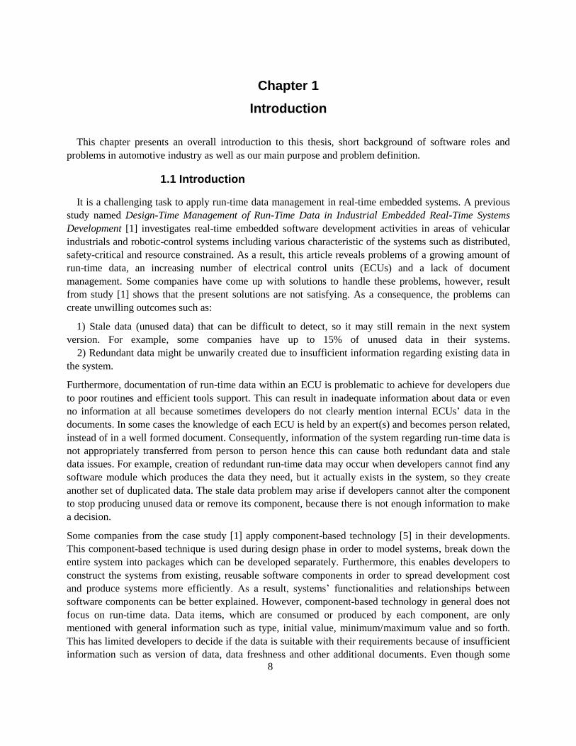
1.1 Introduction
It is a challenging task to apply run-time data management in real-time embedded systems. A previous
study named Design-Time Management of Run-Time Data in Industrial Embedded Real-Time Systems
Development [1] investigates real-time embedded software development activities in areas of vehicular
industrials and robotic-control systems including various characteristic of the systems such as distributed,
safety-critical and resource constrained. As a result, this article reveals problems of a growing amount of
run-time data, an increasing number of electrical control units (ECUs) and a lack of document
management. Some companies have come up with solutions to handle these problems, however, result
from study [1] shows that the present solutions are not satisfying. As a consequence, the problems can
create unwilling outcomes such as:
1) Stale data (unused data) that can be difficult to detect, so it may still remain in the next system
version. For example, some companies have up to 15% of unused data in their systems.
2) Redundant data might be unwarily created due to insufficient information regarding existing data in
the system.
Furthermore, documentation of run-time data within an ECU is problematic to achieve for developers due
to poor routines and efficient tools support. This can result in inadequate information about data or even
no information at all because sometimes developers do not clearly mention internal ECUs‟ data in the
documents. In some cases the knowledge of each ECU is held by an expert(s) and becomes person related,
instead of in a well formed document. Consequently, information of the system regarding run-time data is
not appropriately transferred from person to person hence this can cause both redundant data and stale
data issues. For example, creation of redundant run-time data may occur when developers cannot find any
software module which produces the data they need, but it actually exists in the system, so they create
another set of duplicated data. The stale data problem may arise if developers cannot alter the component
to stop producing unused data or remove its component, because there is not enough information to make
a decision.
Some companies from the case study [1] apply component-based technology [5] in their developments.
This component-based technique is used during design phase in order to model systems, break down the
entire system into packages which can be developed separately. Furthermore, this enables developers to
construct the systems from existing, reusable software components in order to spread development cost
and produce systems more efficiently. As a result, systems‟ functionalities and relationships between
software components can be better explained. However, component-based technology in general does not
focus on run-time data. Data items, which are consumed or produced by each component, are only
mentioned with general information such as type, initial value, minimum/maximum value and so forth.
This has limited developers to decide if the data is suitable with their requirements because of insufficient
information such as version of data, data freshness and other additional documents. Even though some
9
companies have strived to manage their data by using text-based spreadsheet applications, data
dictionaries or other data management tools, they are not capable to manage knowledge regarding run-
time data nor illustrate dependency among data elements. As a result from article [1], the companies have
not successfully applied those tools to solve the data management problems that are occurring in
development life cycle. Consequently, it is difficult to manipulate the run-time data during design time
e.g. addition, removal and searching of existing data. In addition, current data management tools in the
market do not provide graphical visualization which can reveal relationship among data items so
developers cannot simply comprehend roles of each data item or anticipate side effect if a particular data
is altered.
From discussion above, a proper data management is strongly recommended in software development. A
possible solution to deal with the problems is proposed in A Data-Entity Approach for Component-Based
Real-Time Embedded Systems Development [2] suggests that we should focus on run-time data
management during design-time. This approach concerns uniform ways to 1) Document ECU‟s run-time
data. 2) Capture relationships among data items. 3) Automate analysis of data. As a result, developers can
better comprehend the system and avoid inappropriate activities and mistakes during design time.
We have developed a tool based on this Data-Entity approach in order to support developers to be able to
manipulate run-time data items. Run-time data items are graphically visualized and analyzed at design
time with respect to usage, staleness, type checking, data propagation and end-to-end point of view. As a
result, the tool can provide a better understanding of run-time data in the system, manage documentation,
detect stale data and prevent creation of redundancy as well as it can perform data analysis.
1.2 Background
Component Based Software Engineering (CBSE) is a concept used to develop intensive software
system. The concept is about breaking down the entire system into several modules called components.
Each component has a set of related functions and communication interfaces to exchange data with others.
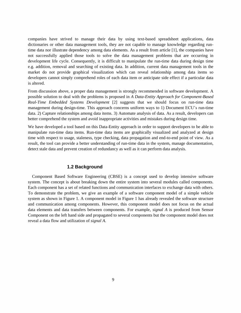
To demonstrate the problem, we give an example of a software component model of a simple vehicle
system as shown in Figure 1. A component model in Figure 1 has already revealed the software structure
and communication among components. However, this component model does not focus on the actual
data elements and data transfers between components. For example, signal A is produced from Sensor
Component on the left hand side and propagated to several components but the component model does not
reveal a data flow and utilization of signal A.

10
Signal A
ModeChange
Component
Follow
ComponentData flow
Actuator
Component
Figure 1: Component model and real-time data item
Data usage of each component, both consumption and production, is not considered as a main objective
in component model. Usually, those data are described by its name and few attributes such as type, initial
value or worst case execution time. Whenever we want to reuse signal A we might have to spend more
time in the component model to find which component produces signal A. In addition, if a component
which produces Signal A was not found but it actually exists then the creation of new component causes
redundancy. Furthermore, it is not easy to follow a data flow of Signal A, emphasized as a blue line in
Figure 1. The component model does not provide detailed information about the data flow nor in depth
information and properties about specific data items. We can obviously see the Signal A is consumed by
ModeChange component but the rest of its consumption are not intuitively presented.
Data management tools for embedded systems such as UniPhi[12] and Visu-IT [13] can almost support
developers to be able to focus on run-time data items during design time and these tools are compatible
with component-based technique. Visu-IT has an ability to trace data flows so developers can see
relationships of data items in the system. However, this feature presents the relationships by non-graphical
technique; hence, graphical visualization should be taken into account to assist developers to better draw
inferences about relationships between data items. In general, graphical visualization is a technique to
present raw data in various types such as diagram, picture, map, graph, animation and so forth. This
technique enhances human‟s perception to get understand communication in a better way. An obvious
11
example of graphical visualization used in computer systems can be seen in spreadsheet applications
which can summarize and visualize data of cells in forms of pie chart, bar chart or graph. Consequently,
we can now see an overview of data better than the data written as a table.
1.3 Problem definition
From a scenario above we define our problems as follows:
1. A non-graphical presentation of the relationship between run-time data that is produced and
consumed throughout a system (data flow), is hard for developers to comprehend the system.
2. With current non-graphical presentation of run-time data and its relationship, it is difficult to
navigate and find information such as data dependencies. This could result in unused data (stale
data) which is difficult to detect and remove from the system.
3. Insufficient run-time data documentation can result in unwarily produced and redundant data.
4. Component based technology does not support analysis of run-time data. This can lead to
difficulty to detect erroneous data utilization at design time.
1.4 Contribution
The concept of run-time data management in real-time embedded system at design time named Data
Entity approach was introduced in previous study [2] which prioritizes a role of data management at top
level during design time. Therefore, the main purpose of this thesis is to enhance the data entity approach
by creating a tool with an intuitive graphical user interface to enable developers to create, update, remove
run-time data items and also to explore data items‟ properties, usage and interrelationship with graphical
visualization feature as well as to perform data analysis at design time.
We have applied the graphical visualization technique to present run-time data in a form of graph. A set of
nodes represents software components also their run-time data‟s attributes. Relationships among software
components regarding run-time data aspect are illustrated as a set of edges with directions that can state
whether they are being consumed or being produced.
We can now see an overview of data flows so developers may comprehend the system in a shorter time.
Developers can explore relationships of data items in the system so they can avoid any side effect which
might occur by modifying the data item. Embedded documents are attached with every run-time data item,
as a result, they can make a decision to remove stale data and avoid creation of redundancy. Furthermore,
our tool can also perform run-time data analysis hence mistakes from improper data utilization can be
detected at design time.

12
1.5 Thesis outline
This thesis firstly start in Chapter 1 with a discussion about problems occurring from the lack of data
management in embedded software development during design time and these problems may lead to
unwanted circumstances. As a result, proper data management tools and techniques are needed to support
developers at design time. Chapter 2 presents background knowledge about software roles in embedded
system focusing on automotive industry as well as current tools and techniques with respect to data
management. Chapter 3 describes a software design technique known as component technology and we
focus on real-time embedded component model named ProCom which influences our tool. Chapter 4
describes a possible solution for run-time data management named Data-Entity approach designed to
support real-time embedded component-based software engineering. Chapter 5 discusses about our tool‟s
features that we take graphical visualization into account to enhance the Data-Entity approach with
additional architectural views based on ProCom component model. Chapter 6 presents how we have
implemented our tool. This explains our tool‟s design from database tables, software structures to
development techniques. Chapter 7 presents our tool‟s capabilities with intuitive methods to explore the
system based on run-time data items and help developers to avoid inappropriate activities and mistakes
during design time. Lastly, Chapter 8 concludes what we have done so far.
13
Chapter 2
Automotive industry and software development
This chapter presents some background knowledge and the role of software within the automotive
industry.
2.1 Electronic control unit
Computer controlled system has been used within to automotive industry for many years in order to
reduce cost in product line and increase functionality. The cost of wiring is reduced by replacing
traditional wiring with a communication network which is described in the next section. The complexity
of modern functionality such as airbag, navigation system and anti-lock braking system (ABS) are
impossible to perform by pure mechanics but can be done by a computer system [9]. The revolution of
applying electronic control units (ECUs) in vehicles began when emissions laws were enacted to reduce
the pollution from exhausts. In the early stages, an ECU was only performing tasks such as adjusting the
quantity of air/fuel injected into each cylinder or the spark timing in an engine. Nowadays, a modern ECU
is not only used to calculate amount of air/fuel injection but also ignition timing, variable valve timing
(VVT), the level of boost maintained by the turbocharger (in turbocharged cars), and other peripherals e.g.
ABS, air bag system, navigation system, adaptive cruise control system. A modern ECU might contain 32-
bit, 40 megahertz microprocessor which apparently seems to be powerless but it is enough for running
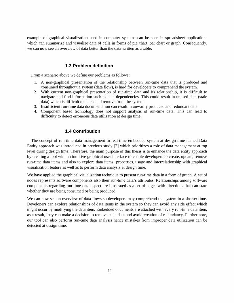
optimized software within its functionalities. An ECU usually appears in a shape as shown in Figure 2. It
has an interface with a number of pins provided a communication with other elements for gathering
information of sensors and providing control to actuators.
Figure 2: Electronic control system [www.r31skylineclub.com]

14
An ECU typically uses closed loop control which is a process that consists of compartments that needs
to be controlled and of controlling elements such as actuators, sensors, regulators or controllers. As
mentioned above that there are many different types of ECU available in a vehicle. They often work
together for a single objective thus it is unavoidable to exchange information and communicate among
them.
2.2 Communication between ECUs
In the past, an ECU had to be directly connected to another ECU by an individual wire. This means
adding new ECU is also increasing numbers of wires. As a consequence, fuel is increasingly consumed by
excessive weight. Furthermore, new innovative features in vehicle do not function alone, instead they
cooperate with other ECUs also known as distributed system therefore the communication among them
are obligatory. Today, a vehicle may consist of a hundred ECUs so this might lead to a big problem such
as complexity of communication or excessive weight from individual wires that link every ECU together.
Fortunately, there are solutions to control a communication used in an embedded system [3], such as
Control area network (CAN) and, Time-Triggered Protocol (TTP), which centralize all communications
into a single network so bunches of wires can be removed. In some cases, one car can have more than one
network such as high speed network and low speed network shown in Figure 3. The network technology
does not only reduce excessive weight and cost problems but also help us to achieve non-functional
requirement such as safety, reliability and availability. Therefore, the system can be developed in much
more efficient way. Analysis of data traffic between these ECUs in the vehicle on the communication
network is one additional sophisticated feature which enables us to improve system performance.
Figure 3: CAN bus [http://www.renesas.eu]

15
2.3 Embedded Software role in automotive industry
Nowadays, Software in automotive industry has become a key factor for the innovative functionality
[9]. According to a study by Mercer Management Consulting and Hypovereinsbank [10], in the year 2010,
software cost will be 13% of the production costs of a vehicle. The cost of developing software has
dramatically increased from the year 2000 as illustrated in Figure 4. The benefits of using software logic
over the dedicated hardware enable vehicle industry to reduce cost, weight and gain higher quality. For
instance, in order to develop an ignition control unit for several vehicle models, we can alter the software
code depending on each model instead of manufacturing numbers of different hardware for every vehicle-
model. Also in this case we can achieve higher quality by better software designing and software testing
approaches. For a new functionality, by software we may integrate the existing modules into a new multi-
functional system. For example, a GPS navigation system can calculate approximated time to the
destination with cooperation from other existing ECUs in the vehicle to gather data such as current vehicle
direction and speed.
Figure 4: Software role in 2010
Few years ago automotive manufacturers considered an ECU in a vehicle as a single unit. They
specified and ordered ECU‟s as black boxes from various suppliers. After the delivery of samples, they
also tested them as black boxes. For the automotive manufacturer, this procedure has a disadvantage that
the software has to be developed again for each new project, if the supplier is changed [11]. This will
result in both wastage of time and cost. Hence we should follow requirements for the development of
reusable software as follows [16]:
“
Reusable application software components must be hardware independent.
Interfaces of the software components must be able to exchange data both locally on an ECU
and/or via a data bus.
16
Developing reusable software, future requirements to the function have to be considered.
Code size and execution time of the software components must be minimized during the
development of reusable software. Both resources are expensive due to mass production of
parts in the automotive industry.
”
System developers need not only to consider those issues, but also requirements engineering [8]
becomes another aspect which should be taken into account. In order to produce a completely new
innovative functionality for a car, we have to find clear details of a new software part which includes both
functional (e.g. input/output, timing constraints) and non-functional (e.g. reliability, safety) requirements.
2.4 Existing data management tools in embedded system
development
There are many commercial data management tools available in the market. However, we are interested
in the functionality of the tools with respect to real-time embedded software development and run-time
data management at design time.
2.4.1 UniPhi
UniPhi [12] is an add-on application for an embedded development environment named Simulink. This
add-on focuses on run-time data by providing data dictionary for data items in the system and allows its
users to choose a signal (data) from the database shown in Figure 5 or, if the signal does not exist, the
users can add it. Hence, this will prevent common bugs in an early phase. This tool also facilitates a
developer to manage system variable and calibration. UniPhi offers simulation and testing activity prior to
code generation and eliminates signal lines between individual blocks to exchange data. In Figure 5,
signals are stored in database and used by both Application and Plant layers. The Signals associate with
system models so if signals are modified then the models will be automatically changed as well. Even
though a problem of lacking documentation for run-time data can be partially solved but it still cannot
solve problems includes obsolete documents, unused data (stale data), duplicated data (redundancy) and
type mismatch.

17
Figure 5: An overview of the UniPhi tool suite
According to our purpose based on data items, UniPhi provides a Data Dictionary which contains
signals‟ attributes and information. The tool presents data in customizable data dictionary thus data can be
grouped by signal or category as shown in Figure 6. UniPhi also enables user to trace usage of each data
item from components as illustrated in Figure 7 below. It can tell developers which components are using
this signal.

18
Figure 6: Data dictionary available in UniPhi
Figure 7: Trace of signal utilized in UniPhi
19
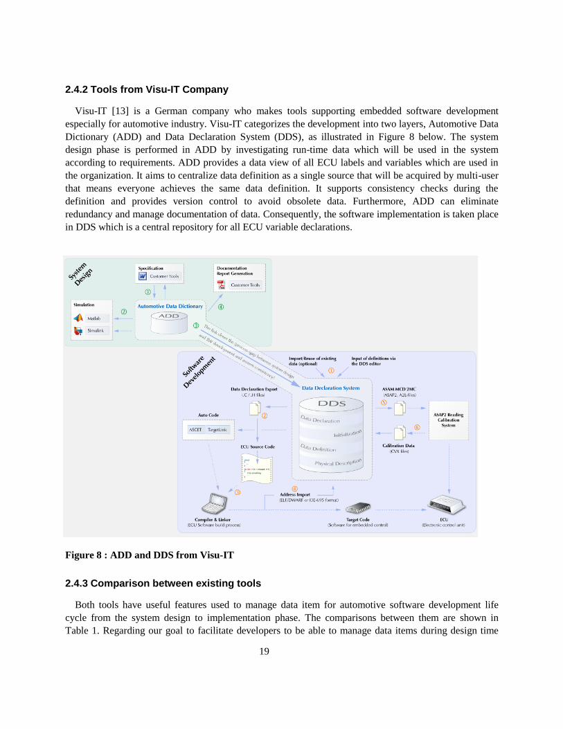
2.4.2 Tools from Visu-IT Company
Visu-IT [13] is a German company who makes tools supporting embedded software development
especially for automotive industry. Visu-IT categorizes the development into two layers, Automotive Data
Dictionary (ADD) and Data Declaration System (DDS), as illustrated in Figure 8 below. The system
design phase is performed in ADD by investigating run-time data which will be used in the system
according to requirements. ADD provides a data view of all ECU labels and variables which are used in
the organization. It aims to centralize data definition as a single source that will be acquired by multi-user
that means everyone achieves the same data definition. It supports consistency checks during the
definition and provides version control to avoid obsolete data. Furthermore, ADD can eliminate
redundancy and manage documentation of data. Consequently, the software implementation is taken place
in DDS which is a central repository for all ECU variable declarations.
Figure 8 : ADD and DDS from Visu-IT
2.4.3 Comparison between existing tools
Both tools have useful features used to manage data item for automotive software development life
cycle from the system design to implementation phase. The comparisons between them are shown in
Table 1. Regarding our goal to facilitate developers to be able to manage data items during design time

20
with respect to CBSE, we are going to develop our tool based on the ideas of data management from these
tools and also add more features which are not in both of them.
Table 1: Features of UniPhi and Visu-It
Tool Version control of
data
Redundancy
check
Documentation of
data
Trace data flow
UniPhi No No Yes Partially
Visu-It Yes Yes Yes Yes

21
Chapter 3
Component technology for real-time embedded system
This chapter describes component based software engineering (CBSE) both in general and in real-time
embedded systems which is used in automotive industry. We focus on ProCom [4] which have been
developed in Mälardalen University.
3.1 Component technology overview
Component based software engineering (CBSE) was proposed to satisfy needs in the industry of having
reusable software modules so this can reduce cost and time in software development life cycle. There is no
globally accepted definition of a component. Definitions differ due to the approach of the component,
some being more theoretical and others more practical. In theory, Szyperski [5] defines a component as “a
unit of composition and it must be specified so that its composition with other components and its
integration to a system is possible and done in a predictable way. [5]” A component must provide and
require a set of interfaces to describe its interaction to other components. The component must also have a
set of executable code which will assist the coupling of interfaces with other components. In practice, a
component is considered as a set of correlated software modules that internally share data and work
together. We can design software system through a component model which provides sets of component
types, interfaces and specifications of patterns for interaction between the components.
3.1.1 Component technology in non real-time system
We can see component software technology in everyday life in various applications from PC
applications, web applications to mobile applications. The most obvious usage of software components is
a graphical user interface (GUI) in Microsoft Windows. Application might be built by predefined GUI
component framework provided by Microsoft such as Textbox, Button, Scrollbar, Menu bar and so forth.
These components have their own set of functions and communication interfaces so in the development,
developers just select and integrate components to build GUI. Not only GUI components that we usually
see but also the component technology has been applied to enterprise application and there are many well
known component frameworks in the market such as COM [33], EJB [34] and CORBA [35]. However,
we do not focus on these technologies because they are not suitable for real-time behaviors which are
mostly applied in automotive software development.
3.1.2 Component technology in real-time system
The correctness of the real-time system does not only depend on the logical result of computation but as
its name “real-time” implies that the timing constraint is considered as an important goal as well. Real-
time system has to be predictable because it must respond to environment upon time so the system is built
as a concurrent program in order to perform many “tasks” in parallel. Tasks can be categorized into
periodic and aperiodic (non-periodic); this means the task that is running in every predefined period and
the task which is activated occasionally as a trigger, respectively. Those tasks have to be well scheduled in
order to meet their deadline and be able to share CPU usage with others.

22
Most real-time applications are deployed in embedded systems which usually have limited resources and
they might have to run for a long time without maintenance. Besides, the applications must perform within
tight timing behaviors e.g. response time and deadline. As a consequence, to design a reusable real-time
component is much more difficult than a non-real-time application. Both running under limited resources
and predictability requirement made it impossible for real-time systems to be developed from existing
component technologies such as COM, JavaBean and CORBA. Moreover, these technologies consume
excessive processing and memory also they do not provide predictable timing schedules for multiple tasks.
There are some component models which are especially created for real-time embedded system, for
example Koala [6], SaveCCM [15] and MARTE [18] which is an extension of UML. However, our thesis
is based on the component model named ProCom [4] which is developed in Marladalen University and we
implement our tool to support this component model.
3.2 ProCom
There are several existing component technologies for real-time embedded system, however, we focus
on ProCom [4] component model which has a potential to enhance an embedded software component
development. ProCom comes with four major objectives as follows : “(i) the ability of handling different
needs which exist at different granularity levels; (ii) coverage of the whole development process; (iii)
support to facilitate analysis, verification, validation and testing; and (iv) support the deployment of
components and the generation of an optimized and schedulable image of the systems. [4]” ProCom
component model is extracted into two abstract layers in order to cover the entire development process of
the system. An above layer called ProSys is used for modeling independent distributed components and a
lower level layer named ProSave is used for modeling and describing control functionality of the
component.
3.2.1 ProSave
In ProSave, abstraction of tasks and control loops are modeled as interaction with the system
environment by either actuator or sensor elements. The ProSave component encapsulates internal data and
functionality with well-defined interface. Therefore, we can reuse a ProSave unit with respect to its
interfaces. The ProSave component is based on pipe-and-filter architectural style thus data is considerably
separated with control flow.
ProSave component is a port-based style so it contains both sets of input and output ports. A port is
categorized into two types which are:
1. Data port which is used to store information. Data input port acquires information from other
components and then, after the computation, the component produces results which are retained at
data output port so as to be consumed as an input by other components. Data port is represented
by rectangle shape shown in Figure 8.
2. Trigger port, controls the activation of components. Trigger port is represented by triangular
shape illustrated in Figure: 9. It can be either input trigger on the left that receives activation
signal or output trigger on the right that sends signal to active other components.
23
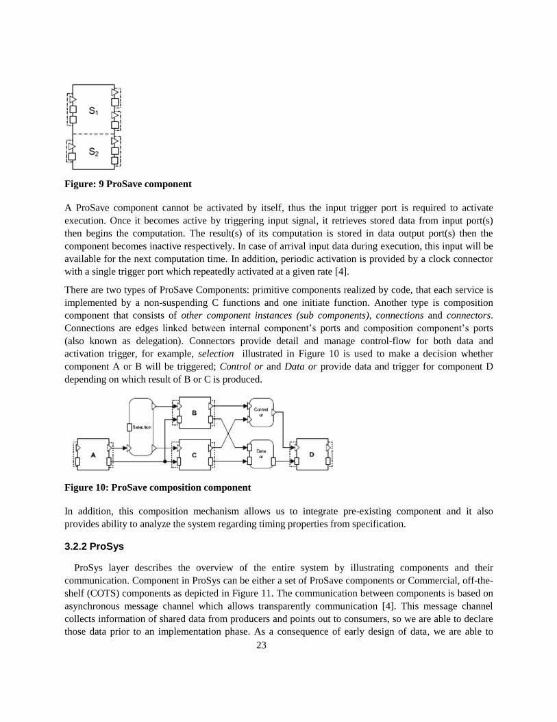
Figure: 9 ProSave component
A ProSave component cannot be activated by itself, thus the input trigger port is required to activate
execution. Once it becomes active by triggering input signal, it retrieves stored data from input port(s)
then begins the computation. The result(s) of its computation is stored in data output port(s) then the
component becomes inactive respectively. In case of arrival input data during execution, this input will be
available for the next computation time. In addition, periodic activation is provided by a clock connector
with a single trigger port which repeatedly activated at a given rate [4].
There are two types of ProSave Components: primitive components realized by code, that each service is
implemented by a non-suspending C functions and one initiate function. Another type is composition
component that consists of other component instances (sub components), connections and connectors.
Connections are edges linked between internal component‟s ports and composition component‟s ports
(also known as delegation). Connectors provide detail and manage control-flow for both data and
activation trigger, for example, selection illustrated in Figure 10 is used to make a decision whether
component A or B will be triggered; Control or and Data or provide data and trigger for component D
depending on which result of B or C is produced.
Figure 10: ProSave composition component
In addition, this composition mechanism allows us to integrate pre-existing component and it also
provides ability to analyze the system regarding timing properties from specification.
3.2.2 ProSys
ProSys layer describes the overview of the entire system by illustrating components and their
communication. Component in ProSys can be either a set of ProSave components or Commercial, off-the-
shelf (COTS) components as depicted in Figure 11. The communication between components is based on
asynchronous message channel which allows transparently communication [4]. This message channel
collects information of shared data from producers and points out to consumers, so we are able to declare
those data prior to an implementation phase. As a consequence of early design of data, we are able to

24
validate type checking of data items being utilized between producers and consumers, to replace a
producer/consumer if its specification meets the requirement given in a message channel, and to reuse
existing component if we already have a component that fits with the specification of the message
channel.
Figure 11: ProSys component
Since ProCom is a component model, we disregard physical communication layer thus a message
channel is just an abstract so it does not exist in real system. In Figure 12, a message channel is a
representation of a single signal (run-time data) from only one producer but, on the other side, it can be
obtained by several consumers. This message channel mechanism is a key to achieve run-time data
management which will be explained in the next chapter.
Figure 12: ProSave message channel

25
3.3 AUTOSAR
Although we have decided to rely on ProCom but there is a standard software framework widely used in
automotive software system which is named AUTOSAR (Automotive Open System Architecture). It was
jointly founded by automobile manufacturers, suppliers and tool developers in 2002 [27]. AUTOSAR
system architecture can be determined as Component based application layer and Basic Software layer
illustrated in Figure 13.
Figure 13: AUTOSAR System Architecture
An AUTOSAR Runtime Environment (RTE) behaves like an operating system for application layer.
RTE provides infrastructure services such as component instantiation, communication among
components, hardware access, memory management and so forth. Hence, software developers may only
focus on application layer in order to create new software. A component in AUTOSAR is a unit of
execution which is also a port based alike. Ports of AUTOSAR software components are defined as type-
require (R-port) or type-provide (P-port) [28] and these ports are connected through interfaces and they
exchange information by Virtual Function Bus (VFB) at application level. An AUTOSAR software
component can be a small piece of functionalities or a larger composite component but the AUTOSAR
software component has to be atomic which means it cannot be distributed over several AUTOSAR ECUs
[29].

26
During software component design phase, run-time data items, which are utilized between software
components, are well described by AUTOSAR‟s standardized exchange format. As a consequence, this
can reduce numbers of different data formats among reusable components from various suppliers; hence
developers can now achieve a clear view of the system regarding run-time data aspect. However, a study
named How the concepts of the Automotive standard „AUTOSAR‟ are realized in new seamless tool-
chains [36] states that “the standard itself does not give support in the modeling process and just partial
support on data consistency”. Since in reality, AUTOSAR model is very complex so this means
additional data management tools are still needed to support developers to focus on run-time data during
design time.
27
Chapter 4
Run-time data management for component based software
engineering
We have introduced commercial data management tools and CBSE [5] concept in previous chapters,
however, as we can see that at design time the component model itself does not fully concern about run-
time data which are both produced and consumed by components. This chapter presents a solution to
manage run-time data at design-time called Data entity approach [2]. The approach in this paper
associates with ProCom [4] component model in particular.
4.1 Data entity approach
Since CBSE does not support developers to clearly understand how run-time data behaves in the system
at design time, the approach named Data Entity [2] suggests a solution to prioritize role of data
management at design time. The Data Entity approach enables design-time modeling, documentation and
run-time data management that are reflected as additional architectural view [17] known as data
architectural view.
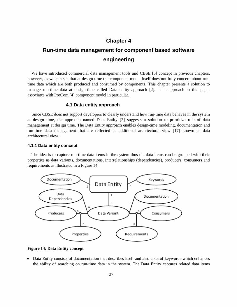
4.1.1 Data entity concept
The idea is to capture run-time data items in the system thus the data items can be grouped with their
properties as data variants, documentations, interrelationships (dependencies), producers, consumers and
requirements as illustrated in a Figure 14.
Figure 14: Data Entity concept
Data Entity consists of documentation that describes itself and also a set of keywords which enhances
the ability of searching on run-time data in the system. The Data Entity captures related data items

28
which are Data Variants. This is an entry for developers to gather information of run-time data in the
system. For instance, whenever developers want to acquire a vehicle speed, they can firstly take a look
at this data entity by giving the keyword “speed”, as a result, they will archive more information of
run-time data as Data Variants related to “speed”.
Data Variant is the actual data item which developers will use. It contains six elements as follows: (i)
Documentation for each particular data item, for example, vehicle‟s speed variables in Km/h and MPH
have their own documentation. (ii) Data Dependencies which contain a set of data entities that the Data
Variant belongs to. (iii) Producers and (iv) Consumers are the representation of components that
existes in ProCom component model described earlier. A Component can act as both producer and
consumer in this approach. In some cases, either producer or consumer might not exist yet. This means
developers can now realize what component they need to develop. (v) Requirements provide
specification for a particular Data Variant with respect to a consumer. The requirement consists of
timing consistency parameter, accuracy and frequency. From any scenario which developers found out
that they have to develop a missing consumer component, this requirement can tell them what they
need to rely on. (vi) Properties are similar to requirements but provide specification of a producer.
Examples of Properties are name, type, size, initial value, minimal value, maximal value and
frequency. In the case of missing a producer developers can use Properties as a requirement to create a
new functionality. In addition, Requirements and Properties are used to match a producer and a
consumer that is the specification of both components must be consistent.
4.1.2 Data entity in practice
Traditionally, software is broken down into components while run-time data is not considerably
concerned as the first priority and then a number of problems mentioned at the beginning might be arisen.
Fortunately, we can solve the problems by establishing the data architectural view that merges ProCom
component model and Data Entity approach together as shown in Figure 15.
Figure 15: Traditional component model and data entity approach
29
Component based software development and data entity approach are associated by central database
that enables both data and component architecture developments exchange information. In the data
development perspective, data entities capture run-time data and these can be manipulated by data
modeling tool.
The run-time data synchronizes with component development under ProCom message channel. This
activity enables a component designer to integrate the components with consistency and design missing
component based on run-time data specification from data entities as a requirement.
The software development is usually performed in parallel from both component development and data
development. For example, once component designers have introduced a skeleton model with some
functions but without complete input/output specification, data developers can now manipulate data
entities based on the current component model, of course with the crude specification of component
model. In the later step, when the data developers achieve clear detailed specification they can provide a
data variant (run-time data item) to fulfill the incomplete specification and then the process is passed back
to a component development. Component designers can now use data items‟ specification to update their
incomplete functions. In the case of developing a new functionality, a component designer can start
looking at the data items produced by existing components. Therefore he/she may reuse them as well. On
the other hand, if the component designer does not find any existing data item that meets his/her
specification then the specification in his/her hand will be the requirement for a new data variant of the
component which has to be implemented afterward.
ComponentProducer
ComponentConsumerB
Data Variant
Property
name,type,size,...
Requirement
wc,bc,frequency,...
ComponentProducerBackup
ComponentConsumerA
MessageChannel
Data entity
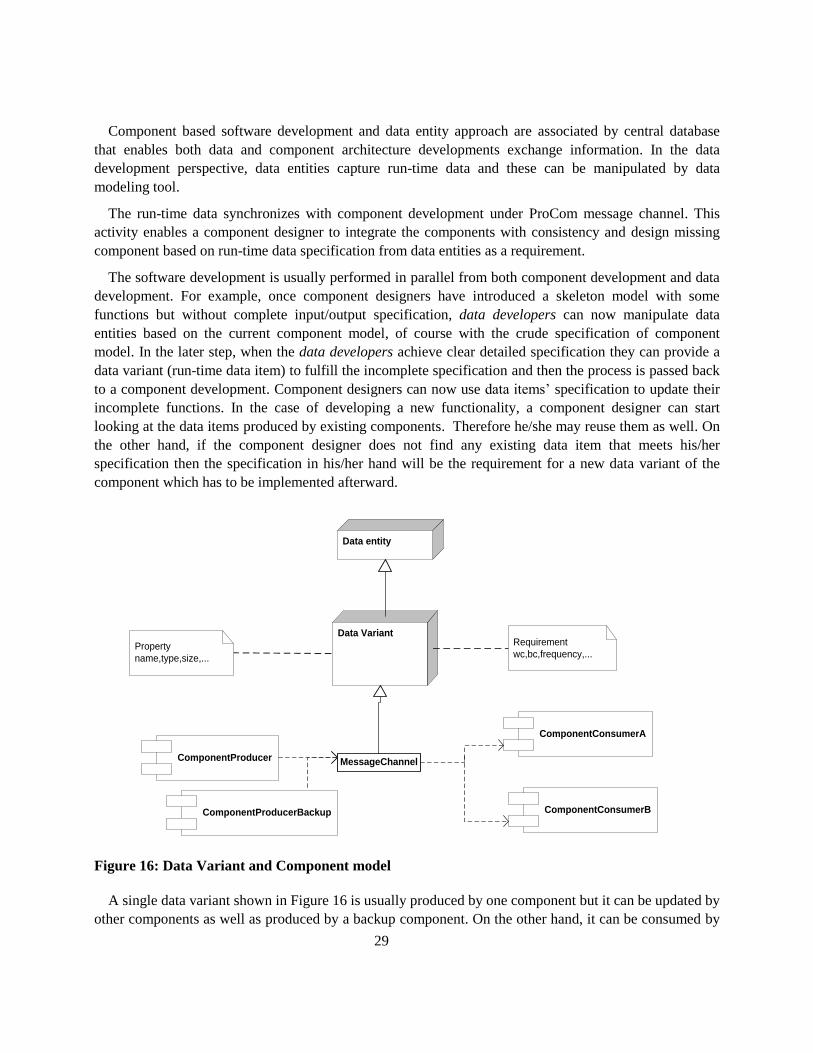
Figure 16: Data Variant and Component model
A single data variant shown in Figure 16 is usually produced by one component but it can be updated by
other components as well as produced by a backup component. On the other hand, it can be consumed by

30
several components. The specification of the data variant is firstly extracted into Property which provides
concrete information of data variant such as name, type (integer, float, character, etc.), size and so forth.
Secondly, it is extracted into Requirement which reveals data variant‟s behaviors such as period, worst
case execution time, best case execution time, frequency and so forth. However, the data variant does not
directly associate with component but it is a representation of run-time data that exists in ProCom‟s
message channel as shown in Figure 17. Both OutPort and InPort are parts of a producer and a consumer,
respectively. Again, one data variant that connects with a message channel can associate to one OutPort (a
backup component is an exception) and it can be consumed by several InPort(s).
OutPort
MessageChannel
InPort
Data Variant
Figure 17: Data variant belongs to message channel
Regarding previous work, a data item and its attributes are stored in database; however, we have applied
object relation mapping (ORM) [20] in order to achieve advantages of object-oriented programming thus
data item‟s compartments and relationships were transformed into UML class diagram as illustrated in
Figure 18 below. Class DeList (Data Entity) contains a set of class DeVariant (Data variant). Both DeList
and DeVariant have each other‟s reference. This means they can refer to the other during run time. Data
variant associates with Requirement, Property and Documentation. These elements also came from the
concept of Data Entity approach.
On the software component side, Class Component is a representation of software component and it
belongs to SystemView determined as a category of a set of components or we can concern as the entire
system. The connectivity between data items and ProCom is held by class Channel which contains
references from both data item and component. A Channel takes place in the middle between DeVariant
and Port and, of course, Port has an association with Component. All of these compartments are
connected; hence we gain a benefit to traverse into all elements which is very useful in implementation
phase.

31
Figure 18: Data Variant’s compartments

32
4.2 Data Analysis
Stale data is one of our problems therefore we must be able to expose any data item which is not in use
any more. A Developer may perceive if any item is no longer used or no one will use it in the future by
checking an item‟s document which is attached with data variant. In addition, data items can be unfulfilled
as they are a consumer but there is no producer connected and vice versa.
Our tool should provide graphical visualization of all data dependencies, both with respect to data
producers and consumers with an analyzing feature to expose unused data or unfulfilled data. Also it
should be able to capture a conflict between consumer and producer. For example, when producer
provides an Integer type but consumer requires Boolean.
Regarding to real-time behaviors, the timing constraint is considered as a data temporal consistency (or
temporal consistency) of data which has two key factors that are an age and a dispersion (of ages).
The age of data is several versions of data. According to continuous data which has been
repeatedly changed, the data is associated with an age. If the age of the data is more than a
predefined threshold then that data becomes outdated thus it needs to be updated. The age of
data, on the other hand, provides the information of the current value regarding the
environment [2]. For instance, A version x of a data item d is a value of the external object
that produces d. Every time the external object changes its value, a new version of d is
generated. Each version x is thus associated with a time interval that specifies when the
version is valid [9].
The dispersion is the difference between ages. The age dispersions of a set of objects
determine whether the objects represent a valid and timely snapshot of the real world
described by them [2].
We can now conclude that the data objects are temporarily consistent if their ages and dispersions are
sufficiently small to meet the requirements of the application. For example, the car‟s speed which is
possibly used in GPS component must not be older than 10 seconds from the present time. Consequently,
these age and dispersion of the data are taken into account when we are approaching to use any real-time
data item. Data variant contains information of real-time behaviors such as period, best case execution
time, worst case execution time, absolute validity and relative validity. We should be able to validate our
data items if they are fulfilled with the requirement. However, at this time ProCom component model does
not fully provide information regarding to absolute and relative validity thus we cannot solve this issue at
the moment but it is possible to deal with in the future.

33
Chapter 5
Visualization of Data Entity approach
We have introduced the Data Entity approach that merges run-time data and software component
technology together; therefore, large quantity of raw-data will have to be taken into account. This chapter
presents our idea to visualize data items‟ properties and their relationship. We will describe our tool‟s
functionalities used to manipulate run-time data items.
5.1 Concept of visualization
Graphical visualization is proposed to enhance capability of the human brain to detect patterns and draw
inferences [25]. Therefore, our tool aims to enable developers to intuitively explore run-time data, their
properties, usage and interrelationship. Our visualization is based on graph theory which consists of nodes
and edges. A set of nodes are data entity, data variant, property and requirement of data variant,
documentation, message channel (derived from ProCom), port and producer/consumer component. An
edge is determined as a connection between two nodes which can be containment, association, providing
and consumption of data.
We should focus on visualizing the data items rather than other elements in the system e.g. ports,
components or channels. The tool has to be able to present or focus on the data items at the beginning.
However, we can also start exploring the system from a data entity or a component.
Start
Data Entity
Perspective
Data Variant
Perspective
Component
perspective
Search item View attributesManipulate
attributes
Figure 19: Starting point of exploring data items

34
Figure 19 above shows the main idea to explore data items which provides several ways to view or
manipulate data items. There are three perspectives focused on data entity, data variant and component.
According to their names, the data entity perspective focuses on any activity correlated with data entity;
data variant perspective focuses on the real-time data items and component perspective provides
information of system components.
Each of these perspectives has the same procedures which are searching, viewing and manipulating
item‟s attributes. In the following description we will call any data entity, data variant, or component as an
“item” and item‟s attributes are the information respected with the item; for instance, a data variant has
attributes as its documentation, property and requirement so a component item has attributes as ports. In
order to explore each item, we can choose an item from the entire list but if there are too many items in the
system then it would be too difficult to see all of them and choose one. Therefore, we have to be able
search the item by giving some keywords which are probably in either item‟s name or description. The
item‟s attributes depend on their type that we have introduced in Chapter 4. For example, when we choose
a data variant, we will see its documentation, property, requirement and the channel that the variant
associates with.
5.2 Activities under exploration of data items
It is not a good idea to only take a look at the item‟s attributes or just to see the relationship among
these items. Therefore, we should be able to manipulate our items such as add, remove and edit.
The activities under Data Entity perspective are:
View all data entities in our system.
View specific data entity
Change name and description.
Add or remove data variant in data entity.
Create or remove data entity. For removal, all data variants will be removed automatically.
Search data entity.
The activities under Data variant perspective:
View all data variants in our system.
View variant‟s interrelationship.
Change name and description.
Add, remove or manipulate its attributes which are Requirement, Property and Documentation.
Connect to Channel or remove from Channel.
Add or remove data variant.
Search data variant.

35
The activities under Component perspective:
View all systems and component.
Search system and component.
View relationship among variants and components.
The tool should be able to visualize the overview of relationship among data items and their
producer/consumer of the entire system. Furthermore, analysis feature should be included in intuitive
method which we have done and will be shown in Chapter 7.

36
Chapter 6
Implementation
This chapter presents how we developed our tool based on concept and idea from previous chapters. We
begin with database which stores information of run-time data items converted from ProCom component
model. Then we present our tool‟s software architecture and finally we show results what the tool can do.
6.1 Relational Database
Database and data used in our tool are influenced from previous work Data Entity Approach [2] and
based on MimerSql [21]. We have nine tables in accordance with Data Entity concept as follows;
Table Delist is known as a container of real-time data variants, which are stored in Table DeVariant. We
can categorize data variants into groups based on their similarity such as values of vehicle‟s speed in km/h
or mph belong to the same category of Delist. Table Requirement, Property and Documentation contain
information of a data variant in detail. Table System and Component are collections of ProSys and
1) Table Delist (Name char(30) , DeListID integer primary key, Description char(50));
2) Table DeVariant (Name char(30), DeVariantID integer, ChannelId integer,RequirementId integer,
Description char(150), DeListID integer, primary key(DeVariantID));
3) Table Documentation (Name char(30), DocumentationID integer,DeVariantID integer, Doc
char(255), primary key(DocumentationID));
4) Table Requirement (RequirementID integer, Desc char(255), Frequency integer, Accuracy integer,
Period integer, Bc integer, Wc integer, Avi integer, Rvi integer, primary key(RequirementID));
5) Table Property (Name char(30), PropertyID integer,DeVariantID integer, Type char(20), Size
integer, Scope char(20), Scale char(20), InitValue integer, MinValue integer, MaxValue integer, primary
key(PropertyID));
6) Table Channel (ChannelId integer,RequirementId integer, Description char(255), Name
char(30),primary key (ChannelId));
7) Table System (Name char(30), SystemID integer, Description char(50), primary key(SystemID));
8) Table Component (Name char(30),ComponentID integer ,OwnerSystemId integer, ModelFileName
char(30), ModelType char(10), RealisationFileName char(30), RealisationEntry char(30), Description
char(30), primary key(ComponentID));
9) Table Port (PortID integer,Name Char(30), ComponentId integer, channelId integer, Mode char(30),
Type char(20), SetPort char(20),InPort boolean, Description char(30), primary key(PortID));
Table 2: List of tables used in our tool

37
ProSave respectively. Table Port obviously stores information of a component‟s ports and it provides a
link between itself and Table Channel, which conforms to a message channel in ProCom.
These tables have their integrities, Entity integrity, as a primary key so it guarantees that we will not
face with duplicated data objects. They also have a Referential integrity as foreign key which is used to
refer between data objects and held the deletion rule; for instance, when we delete any DeList, its variants
will be deleted as well. Noted, the actual data used in our application is prepared by converting ProCom‟s
components information to database and this is made by another tool proposed in Data-Entity Approach
for Component-Based Real-Time Embedded Systems Development [2].
6.2 Object/Relational Mapping
On one hand, a relational database is very powerful and it is widely use as the main persistence storage.
However, a newer trend of software development is based on Object-Oriented approach. This means a
relational database can only store scalar value but it cannot store non-scalar value. For instance, when we
want to store information of DeVariant, which has reference data type attributes, we must convert all
attributes into scalar values such as string or integer.
To convert DeVariant‟s attributes, like Requirement or Property, we have to either manually write a
bunch of SQL lines or make a function in order to parse information from the objects to scalar value.
Object-relational mapping [22] (ORM) was introduced to handle connectivity between application and
database as a middle wear which provides and accepts data in term of object rather than record or table
form (also known as result-set).
It is unnecessary to apply ORM with a small application but when we are considering about session
management, transaction, security or authority, these issues might bring excessive work load to deal with.
Another benefit of using ORM is portability. At the very beginning of implementation phase we used
another database named HSSQL, which is light weight and easy to use, just to use for testing if our
software design works correctly. Since we have been using ORM, we do not need to reconfigure our
application code but just change some configuration files that takes less than 10 minutes and then we are
ready to work on MimerSQL [21] or other DBMS.

38
DeList
Mimer SQL
Data Access Object
manager
(Hibernate)
DeVariance
......
SubSystem
Java code
Figure 20: Object Relational Mapping
Figure 20 illustrates an idea of using ORM. The elements under cloud shape are known in ORM jargon
as Entity which contains data members and its accessors/mutators (getter/setter). Data Access Object
Manager provides a set of helper classes used to manipulate data without referring to a single line of SQL.
For instance, DeVariant has name, description and references to other objects e.g. DeList, Channel,
Property, Requirement and Documentation. It has getters and setters for all members. If we want to
retrieve DeList which is a parent of DeVariant, instead of executing SQL command like “select DeList
where DeListId = DeVariant.DeListId from DeList”, we can just call “deVariant.getDeList()”. Figure 21
below shows an example of Entity class. In addition, we can traverse in a chain of relationship among
items. For example, if we want to know which sub component consumes this data variant, we can
investigate through message channel connected to the variant then get port(s) from channel; as a
consequence, we can now reach component which has port(s) associates with this channel. This example
of exploration will be explained clearly in Chapter 6.

39
public class DeVariant implements Serializable {
private Channel channel;
private DeList deList;
private String description;
private String name;
public void setDeList(DeList deList) {
this.deList = deList;
}
public DeList getDeList() {
return deList;
}
public Channel getChannel() {
return channel;
}
public void setChannel(Channel channel) {
this.channel = channel;
}
public String getDescription() {
return description;
}
public String getName() {
if(name!=null){
return name.trim();
}
else{
return "";
}
}
public void setName(String name) {
this.name = name;
}
public void setDescription(String description) {
this.description = description;
}
}
Figure 21: Example of ORM entity
40
<hibernate-mapping package="model">
<class name="DeVariant" table="DeVariant">
<id name="DeVariantId">
<generator class="increment" />
</id>
<property column="Description" generated="never" lazy="false"
name="description" />
<property column="Name" generated="never" lazy="false"
name="name" />
<one-to-one name="documentation" class="Documentation"
lazy="false" cascade="all" property-ref="deVariant" />
<one-to-one name="property" class="Property" lazy="false"
cascade="all" property-ref="deVariant" />
<many-to-one name="channel" class="Channel" column="ChannelId"
lazy="false" cascade="none" unique="true" not-null="false"
/>
<many-to-one name="requirement" class="Requirement"
column="RequirementId" lazy="false" cascade="save-update"
unique="true"
not-null="false" />
<many-to-one name="deList" column="deListID"
not-null="true" cascade="save-update" lazy="false" />
</class>
</hibernate-mapping>
6.2.1 Hibernate
Nowadays, there are many ORM frameworks with Java support e.g. EclipseLink [30], Java Data
Objects [31], iBATIS [32] and so forth. However, we chose Hibernate because it is free under LGPL open
source license, popular and easy to find documentation. Hibernate generates SQL commands for us,
eliminates JDBC result set handling and object conversion, and keeps our application portable to all SQL
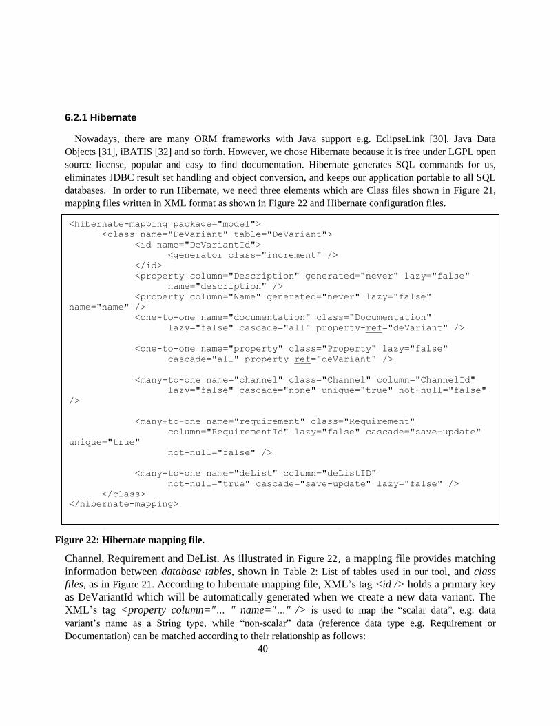
databases. In order to run Hibernate, we need three elements which are Class files shown in Figure 21,
mapping files written in XML format as shown in Figure 22 and Hibernate configuration files.
Class file named “DeVariant” in Figure 21 does not show all attributes and methods because it
has too many lines of code. However, DeVariant actually consists of Documentation, Property,
Channel, Requirement and DeList. As illustrated in Figure 22, a mapping file provides matching
information between database tables, shown in Table 2: List of tables used in our tool, and class
files, as in Figure 21. According to hibernate mapping file, XML‟s tag <id /> holds a primary key
as DeVariantId which will be automatically generated when we create a new data variant. The
XML‟s tag <property column="… " name="…" /> is used to map the “scalar data”, e.g. data
variant‟s name as a String type, while “non-scalar” data (reference data type e.g. Requirement or
Documentation) can be matched according to their relationship as follows:
Figure 22: Hibernate mapping file.

41
One-to-one is the simplest relationship between two objects.
<one-to-one name="documentation" class="Documentation" lazy="false" cascade="all"
property-ref="deVariant" />
from the one-to-one tag above, our class DeVariant has Documentation as a data member which
is referred by the variable named "deVariant". And of course, the mapping file of class
Documentation has to point back to DeVariant as well.
Many-to-one describes a relationship of more than two objects. This term is quite confusing
because it is also used to map one-to-one relationship due to technical issues of Hibernate. For
more information of Hibernate mapping relationship such as One-to-many and Many-to-many
can be found in Agile Java development with Spring, Hibernate and Eclipse [22]. By the way,
data variant associates with data entity by a variable named "deList" which refers to data entity
by "deListID". On the other way around, a class file and a mapping file of DeList hold a set of
DeVariant as well.
Some additional commands in the mapping file, such as lazy="false", cascade="save-update",
unique="true" and so forth, can be used to gain a better control of our data manipulation for instance, the
lazy command tells Hibernate whether to perform lazy fetching or not and the cascade command is used
to control referential actions of database.
Once we have done all mapping files and class files we still need façade classes which provide convenient
access to our class files. These façade classes are also known as Data Access Object Manager depicted in
Figure 23. DAO manager of DeVariant provides functions as follows:
getDeVariants(): retrieves all data variants at once.
getById(int id): retrieves single data variant by a unique key.
getByExample(DeVariant variant): retrieves a list of data variants. For instance, if an
input refers to any data entity then the result will be all data variants associated with the giving
data entity.
save(final DeVariant variant): updates an existing data variant or creates new one, if
the id of a given input does not exist.
delete(DeVariant variant)and deleteById(final int id): deletes a data variant
from database.
search(final String keyword): searches a given keyword in both description and name.

42
public class DeVariantDao extends HibernateDaoSupport {
public List<DeVariant> getDeVariants(){
return getHibernateTemplate().find("from DeVariant");
}
public DeVariant getById(int id){
return (DeVariant)getHibernateTemplate().get(DeVariant.class, id);
}
public List<DeVariant> getByExample(DeVariant variant){
return getHibernateTemplate().findByExample(variant);
}
public void save(final DeVariant variant){
if(variant.getDocumentation()!=null)
variant.getDocumentation().setDeVariant(variant);
if(variant.getProperty()!=null)
variant.getProperty().setDeVariant(variant);
if(variant.getChannel()!=null)
variant.getChannel().setRequirement(variant.getRequirement());
getHibernateTemplate().saveOrUpdate(variant);
getHibernateTemplate().flush();
}
public void delete(DeVariant variant){
getHibernateTemplate().delete(variant);
}
public void deleteById(final int id) {
DeVariant c = (DeVariant)
getHibernateTemplate().get(DeVariant.class, id);
delete(c);
}
public List<DeVariant> search(final String keyword) {
return getHibernateTemplate().executeFind(new HibernateCallback() {
@Override
public Object doInHibernate(Session session)
throws HibernateException, SQLException {
Criteria criteria =
session.createCriteria(DeVariant.class);
criteria.add(Restrictions.or(
Restrictions.like("description",
keyword, MatchMode.ANYWHERE).ignoreCase(),
Restrictions.like("name", keyword,
MatchMode.ANYWHERE).ignoreCase()));
return criteria.list();
}
});
}
} Figure 23: Data Access Object Manager

43
6.3 Inversion of control by Spring framework
We already have nine database tables thus we also have nine Entity classes (shown in Figure 21:
Example of ORM entity) plus nine DAO Manager classes (shown in Figure 23: Data Access Object
Manager) and also nine hibernate mapping files. Therefore, to manually hook up or connect these
components and configuration files may acquire excessive work; of course, we will lose both dependency
among components and resource handling. Besides, instantiation of all database service classes will be out
of control. According to Inversion of control (IoC) approach proposed by Martin Fowler [20], we do not
need to create or instantiate our objects but we only describe how those objects should be created, as a
consequence, we do not need to strictly connect components in our code files. For instance, if we want to
use some services from Hibernate in DeVariantDao in order to manipulate a DeVariant, we will not use a
keyword new as follows;
Assuming that a reference named service provides some data services from Hibernate and this example is
a conventional style to instantiate the service. In order to avoid this, we have to separate an application's
configuration and dependency specification from the actual application code. So we are going to let
Spring Framework [23] binding our components and services; this methodology is known as dependency
injection [20]. According to the example above, a reference service will not be instantiated inside of this
class but it will be instantiated and injected from outside.
Spring Framework is an open source framework created to eliminate the complexity of enterprise
software development. Spring comprises with many useful features but in our case, we are going to use
two features which are Spring ORM and Spring DAO. These features provide integration with Hibernate
by enabling resource management and transaction strategy. As we mentioned above about Hibernate
mapping files, Entity classes and DAO manager classes, we can now integrate them as depicted in Figure
24: Spring ORM. There is one more additional configuration file named application context (illustrated in
Figure 24 and Figure 25) and it is created to connect everything together. This application context contains
information of database connection, Hibernate session factory and dependency injection for DAO
managers as shown in Figure 25.
public class DeVariantDao extends HibernateDaoSupport {
public List<DeVariant> getDeVariants(){
HibernateDataBaseService service = new
HibernateDataBaseService();
return service.getData();
}
}

44
Spring ORM
Database
DAO manager
(e.g. DeVarianceDAO)
Entity
(e.g. DeVariance)
Hibernate mapping filesApplication context
UI
Figure 24: Spring ORM

45
<?xml version="1.0" encoding="UTF-8"?>
<!DOCTYPE beans PUBLIC "-//SPRING//DTD BEAN//EN" "spring-beans.dtd">
<beans>
<bean id="dataSource"
class="org.springframework.jdbc.datasource.DriverManagerDataSource">
<property name="driverClassName" value="com.mimer.jdbc.Driver" />
<property name="url" value="jdbc:mimer:tcp://localhost:1360/RTDB"
/>
<property name="username" value="DEMETA" />
<property name="password" value="DEMETA" />
</bean>
<bean id="sessionFactory"
class="org.springframework.orm.hibernate3.LocalSessionFactoryBean">
<property name="dataSource" ref="dataSource"></property>
<property name="useTransactionAwareDataSource" value="true"
/>
<property name="mappingResources">
<list>
<value>Channel.hbm.xml</value>
<value>Port.hbm.xml</value>
<value>DeVariant.hbm.xml</value>
<value>DeList.hbm.xml</value>
<value>Documentation.hbm.xml</value>
<value>Property.hbm.xml</value>
<value>Requirement.hbm.xml</value>
<value>Component.hbm.xml</value>
<value>SystemView.hbm.xml</value>
</list>
</property>
<property name="hibernateProperties">
<props>
<prop key="connection.pool_size">1</prop>
<prop key="hibernate.dialect">
org.hibernate.dialect.MimerSQLDialect
</prop>
</property>
</bean>
<bean id="deVariantDao" class="dao.DeVariantDao">
<property name="sessionFactory" ref="sessionFactory" />
</bean>
<bean id="deListDao" class="dao.DeListDao">
<property name="sessionFactory" ref="sessionFactory" />
</bean>
</beans>
1: Database connection
2: Hibernate mapping files
3: Dependency injection
Figure 25: Application Context

46
According to Figure 25, the first part of application context file explains where and how to connect to
the database. The second part contains information of a feature ORM support by Spring framework. We
actually tell Spring that we are going to establish sessionFactory (it is just a reference name) which
provides data services from both Hibernate and Spring. These services will be used to manipulate and
handle our Hibernate‟s transactions later in our DAO managers. In the third section, Spring is going to
insert sessionFactory into DAO managers; indeed, this action is called dependency injection. We already
have a setter method for session factory in our DAO manager classes so this means the service is
externally injected into DAO managers.
As a result, the service (in our case is sessionFactory) is instantiated and properly set up by Spring and
then it is injected into DAO managers respectively. By doing this, we gain a better control of our services
whenever we want to change something about the service we have no need to recode anything in our class
file. Finally, we will use these DAO managers in visualization development without any database issue
since raw data were transformed into object oriented approach already.
6.4 Unit testing
Every day we modify or add more functionality to our components so we need to ensure that our
components still work properly, therefore, unit testing has been proposed in [24] and it is widely used to
guarantee correctness of the outcome of components after daily build. The basic concept of unit testing is
to define a test suite contains test cases that invoke components‟ functions and check if the results are
matched with predefined requirements. Consequently, we use JUnit as a unit testing tool for our
application. Every DAO manager has its own test case covered every public method (service) which is
used by UI and Visualization modules. Regarding to DAO manager of DeVariant depicted in Figure 23:
Data Access Object Manager, it has seven services as follows:
getDeVariants(),getById(int id), getByExample(DeVariant variant), save(final
DeVariant variant), delete(DeVariant variant), deleteById(final int id)and
search(final String keyword).
A test case of DeVariant DAO manager should have corresponding methods associated with these
seven methods, however, we just give some of testing criteria shown in Figure 26 below. Firstly, JUnit
starts with method setUp()used to initialize our DAO managers, which will be performed by other
testing methods, in this case we are going to show only two examples so we need only Delist and
DeVariant DAO managers. Secondly, we are heading to test the method getById supposed to return a
data object with the same ID as given. Therefore, we perform assertNotNull() to check if the DAO
manager provide an object and then we validate the result if it has the correct ID by using method
assertEquals(new Integer(1),variant.getDeVariantId()).The next one is to verify method
save(final DeVariant variant), it is obvious that we create a new object and ask DeVariant DAO
manager to save then we call assertNotNull() again to verify if the object was saved.

47
Indeed, the example given above is just a part of all test cases so we actually created most of possible
behaviors which might be occurred in our application; for example, whenever we delete any parent data
item then its children must be automatically deleted or we have to validate the result from searching and
so forth. The main advantage of performing this unit testing is reflected as we can implement the other
module with confidence since we will know immediately if something goes wrong thus we can prevent it.
public class TestDeVariantDao {
DeVariantDao variantDao;
DeVariant de;
DeListDao deListDao;
@Before
public void setUp() throws Exception {
/* initiate DAO managers*/
DaoFactory factory=DaoFactory.getDaoFactory();
variantDao = (DeVariantDao) factory.getDao("deVariantDao");
deListDao = (DeListDao) factory.getDao("deListDao");
SessionTransactionManager.start(variantDao.getHibernateTemplate());
}
@Test
public void testGetById() {
DeVariant variant = variantDao.getById(1);
assertNotNull(variant);
assertEquals(new Integer(1), variant.getDeVariantId());
}
@Test
public void testSave() {
de = new DeVariant();
de.setName("test1");
DeList delist= deListDao.getById(1);
de.setDeList(delist);
variantDao.save(de);
// test if we can save the object
assertNotNull(variantDao.getById(de.getDeVariantId()));
}
// Do some more testing
}
Figure 26: JUnit test case

48
6.5 Visualization by JGraph
Until now we have shown our implementation from database design, data service components and
software infrastructure. We already described a concept of graphical visualization in Chapter 5 so in this
section we are going to describe how we visualize real-time data item. We chose JGraph [26] as a drawing
component for our application because it is widely used and well documented. Real-time data items and
their relationships are presented as nodes and edges, respectively. What we do is to plot these nodes and
edges related to raw data from database. The Node and Edge components from JGraph are Java Swing
alike, which means JGraph‟s components derive attributes, functionalities and behaviors from a class
named JComponent of Java Swing. Therefore, we can use them in the same way as Java Swing but these
JGraph‟s component enable us to work with additional features such as connecting nodes and edges
together or attaching raw data with a node then we can retrieve information from each node during run
time.

49
Chapter 7
Visualization of data items
This chapter presents our tool‟s functionalities to visualize run-time data based on an example
component model of a truck system.
7.1 Example system
In order to present our tool‟s capability, we use a truck system as our example. A component model of
the truck system is shown in Figure 27. This truck can follow a black track. It has sensors attached on the
left, the middle and the right where these sensors determine the track. Each sensor consists of 1) a sensor
that returns a raw value in voltage. 2) A derivation which transforms voltage value into scale integer, for
instance, value 0 is black and value 255 is white. 3) A Calibration which provides a boolean value if the
track is black or not. The system has three components which provide sets of commands how the truck
should behave including Find, Follow and Turn. These three components are selected to be performed by
another component named ModeChange. As a consequence, Arbitrator component gathers information
from the components mentioned earlier. The Arbitrator manages throttle data then transfers the data to
ThrottleDetermination component that transforms integer value to voltage and then it sends the signal to a
ThrottleActuator component.
Obviously, data variants of this truck system are captured as values which are produced and consumed
from all components. Data entity is a group of similar variants therefore in this case we can categorize
data entity into six groups as follows:
1. Sensor Left contains all signal values from the sensors on the left of the truck. Including
voltage, integer and Boolean values.
2. Sensor Center contains all signal values from the sensors on the center of the truck. Including
voltage, integer and Boolean values.
3. Sensor Right contains all signal values from the sensors on the right of the truck. Including
voltage, integer and Boolean values.
4. Feedback contains variants regarding throttle data from Turn, Follow, Find and Arbitrator.
5. Throttle contains a variant produced from ThrottleDetermination to ThrottleActuator.
6. State contains a variant regarding the current state that made by ModeChange.

50
SL
Variant SL(volt)
DL
CL
Variant SL (int)
SC
Variant SC(volt)
DC
CC
Variant SL(int)
Variant SL (bool)
Variant SC(bool)
SR
Variant SR(volt)
DR
CR
Variant SR(int)
Variant SR(bool)
Turn
Follow
ModeChange
FeedBackTurn(int)FeedBackFollow(int)
State(int)
Arbitrator
ThrottleFollow(int)
ThrottleTurn(int)
Throttle Determination ThrottleActuator
ThrottleArbitrator(int)
ThrottleDetermination(volt)
Find
FeedBackFind(int)
ThrottleFind(int)
Figure 27: Component model of an example truck system
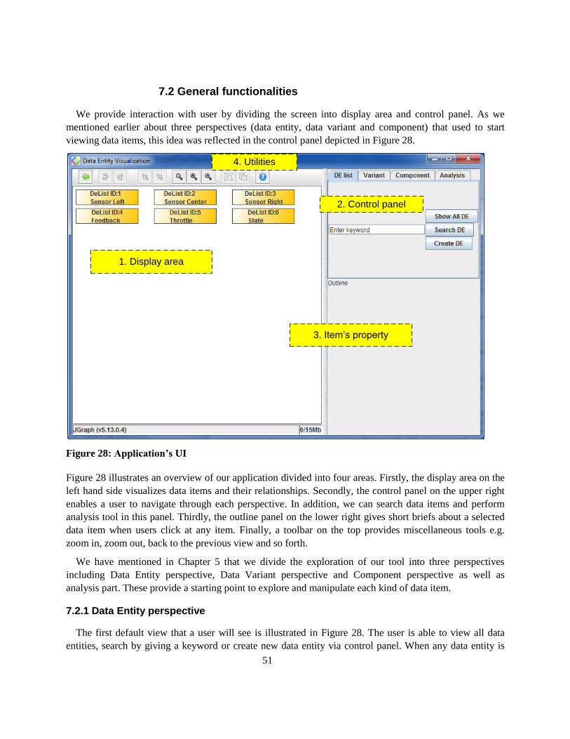
51
7.2 General functionalities
We provide interaction with user by dividing the screen into display area and control panel. As we
mentioned earlier about three perspectives (data entity, data variant and component) that used to start
viewing data items, this idea was reflected in the control panel depicted in Figure 28.
2. Control panel
3. Item’s property
1. Display area
4. Utilities
Figure 28: Application’s UI
Figure 28 illustrates an overview of our application divided into four areas. Firstly, the display area on the
left hand side visualizes data items and their relationships. Secondly, the control panel on the upper right
enables a user to navigate through each perspective. In addition, we can search data items and perform
analysis tool in this panel. Thirdly, the outline panel on the lower right gives short briefs about a selected
data item when users click at any item. Finally, a toolbar on the top provides miscellaneous tools e.g.
zoom in, zoom out, back to the previous view and so forth.
We have mentioned in Chapter 5 that we divide the exploration of our tool into three perspectives
including Data Entity perspective, Data Variant perspective and Component perspective as well as
analysis part. These provide a starting point to explore and manipulate each kind of data item.
7.2.1 Data Entity perspective
The first default view that a user will see is illustrated in Figure 28. The user is able to view all data
entities, search by giving a keyword or create new data entity via control panel. When any data entity is

52
selected in the display area, its information is displayed in an outline panel where a user can alter its name
or description and also the user can delete this entity by clicking on the delete button; as a result, all data
variants belonged to this data entity will be deleted as well.
Figure 29: Additional commands for Data Entity
Additional actions with a data entity can be invoked by right clicking on a specific item as shown in
Figure 29. The popup menu has five commands as follows:
View: this function lets a user to explore data variants of the selected data entity and this action
will display the result as shown in Figure 30.

53
Figure 30: Data Variants in Data Entity
Add variant: a brand new data variant can be inserted under the selected data entity and when a
user perform this function, the creating menu will be popped up as shown in Figure 31. Since data
variant must be belonged to data entity, a user has to choose data entity by giving a keyword to
the search box and select one from the list.

54
Figure 31: Creating new data variant
Remove: this action will delete the selected data entity and its variants.
Create: a user can create new data entity under this command.
Print: the current view will be sent to a printer.
7.2.2 Data Variant perspective
Data variant perspective is actually similar to the previous data entity perspective providing features to
show all data variants, search data variant by looking in only variant‟s name or both name and its
documentation, and create new data variant as depicted in Figure 32.

55
Figure 32: Data Variant perspective
An outline panel provides information of a selected data variant about its name, description, entity
which this variant belongs to, producer(s) and consumer(s). A user is able to connect the selected variant
with an available message channel via a button named “Add channel” and vice versa. The basic actions
performed on data variant such as alter, create and delete can be done in the control tab as well.
In order to explore through data variant, a user has to choose menu view by right clicking on a data
variant then its information will be display as shown in Figure 33.
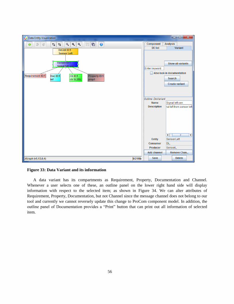
56
Figure 33: Data Variant and its information
A data variant has its compartments as Requirement, Property, Documentation and Channel.
Whenever a user selects one of these, an outline panel on the lower right hand side will display
information with respect to the selected item; as shown in Figure 34. We can alter attributes of
Requirement, Property, Documentation, but not Channel since the message channel does not belong to our
tool and currently we cannot reversely update this change to ProCom component model. In addition, the
outline panel of Documentation provides a “Print” button that can print out all information of selected
item.

57
Figure 34: Outline of data variant’s compartments

58
7.2.3 Component perspective
Similar to both of the previous perspectives, we can start to search or view all of either System or Sub
component. But we cannot create or modify because we are unable to change anything in the ProCom
side. Figure 35 shows the display when performing “show all” function.
Figure 35: System and Component
In order to explore System item, we have two choices which are, firstly, to view all components exist in
selected system and, secondly, to view an overview of the system where we can see every data usage in
the system shown in Figure 36.
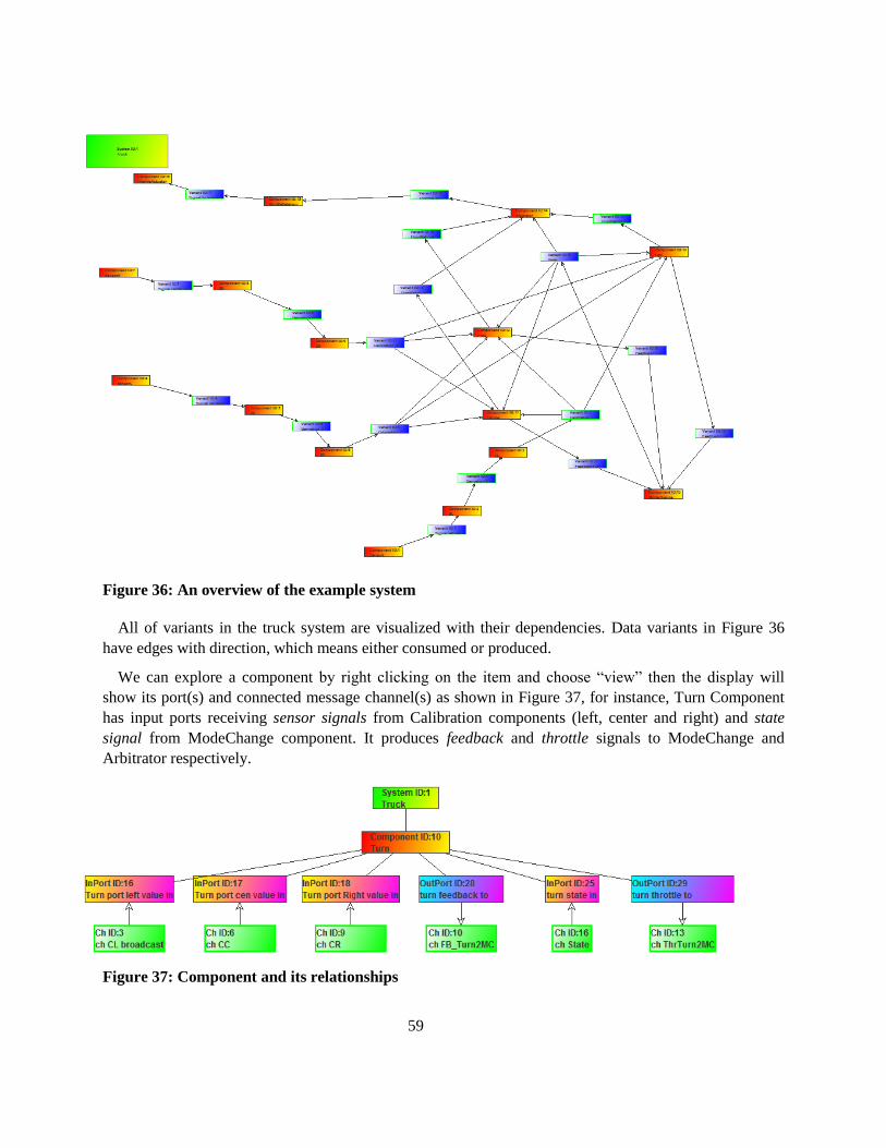
59
Figure 36: An overview of the example system
All of variants in the truck system are visualized with their dependencies. Data variants in Figure 36
have edges with direction, which means either consumed or produced.
We can explore a component by right clicking on the item and choose “view” then the display will
show its port(s) and connected message channel(s) as shown in Figure 37, for instance, Turn Component
has input ports receiving sensor signals from Calibration components (left, center and right) and state
signal from ModeChange component. It produces feedback and throttle signals to ModeChange and
Arbitrator respectively.
Figure 37: Component and its relationships

60
7.3 Intuitive exploration among data items
Since data items are linked together, we are able to freely traverse through all data items from
anywhere. We are going to describe how we explore a data variant depicted in Figure 38.
Figure 38 : Exploration among data items

61
First of all, we choose a data variant then we will acquire its requirement, property, document and
channel. If we want to see where this variant is produced or consumed, we can browse through the
message channel which is associated with the variant. During exploration, we can choose any item to see
its attributes displayed in the outline panel as we mentioned earlier.
The exploration can be done in opposite ways; we can actually start with a component and trace back to
see which data variants are used in this component. In this architectural view, we focus on individual
elements by capturing its consumer and producer but not fully present data flow or dependency. On the
other hand, we also want to reveal data flow (dependency) of the variant thus we created another kind of
view to visualize the data flow as illustrated in Figure 39.
Figure 39: Data flow
Figure 39 shows data flow of selected data variant. On the root top of this tree is a data variant that we
chose to observe. An arrow, which connects data variant and component together, tells us where the
variant is produced or consumed, similar to the previous view. This architectural view enables developers
to see how the variant is utilized so they can learn about relationship with other corresponding elements.
Although this figure is too small but our tool has a zoom in/out feature so we can see this in bigger size.
7.4 Analysis tool
Our tool also provides an ability to analyze data variants that covers type checking, unfulfilled and
unused data variant. Type conflict occurs when both consumer and producer engage to the same data
variant but they exploit different variable types, for instance, consumer requires integer but producer gives
float. This conflict is automatically captured by coloring technique reflected in both data variant‟s border
and message channel‟s border that can be seen in Figure 40. Basically, we imitate the colors from a traffic

62
light which green border means it is fulfilled, red border means it has a conflict, yellow border means
there is no consumer, pink border means there is no producer and grey boarder means the data variant
does not have both producer and consumer.
Figure 40: Coloring technique
Analysis tools
Figure 41: Analysis tools
Figure 41 shows an example of type conflict where a data variant ID: 8 is utilized but the consumer needs
different variable type from the producer. Our tool also provides functions (located in the control tab) to
determine and capture conflict items from the entire system and reveal unfulfilled data variants that are no

63
producer, no consumer and unused at all. According to these features, we can now prevent redundancy
and confidentially eliminate stale data.
Our tool also provides some more trivial features but they could facilitate developers as follows:
Built in printing system: we are able to print a graph or generated documentation of a variant.
Zoom in/out
Automatically sorting data items: Nodes will not be overlapped and we can still manually resize
or move items as well.
Navigate back to the previous steps.

64
Chapter 8
Conclusion
The Data Entity approach [2] prioritizes design-time data management of run-time data when
developing component-based embedded real-time systems. Inspired by the result from this approach, we
have proposed a visualization and analysis tool that facilitates developers to intuitively explore run-time
data items, usage and relationship during design time. Information and dependencies between data items
as well as data flows are graphically illustrated thus it is easier to comprehend the system. We introduce
architectural views to start exploring data items from 1) a group of data items called Data Entity, 2) a
signal utilized by any component known as a Data Variant and 3) a component perspective as. Our tool
exposes information of the items in an intuitive way. Developers are able to draw a conclusion of run-time
data utilized by components and save time to learn the system.
As a consequence, the developers can make a better decision to utilize or manipulate data items
depending on the circumstances; they can eliminate stale data with confidence that the deletion will not
affect entire systems. Run-time data‟s documents are attached with data item thus this can give a clear
view of the data and decrease problems regarding obsolete documentation. The creation of a component,
which attempts to reproduce existing data items, is detected by a searching feature that inform developers
that data which they want to use, already exists in the system. As a result, we can reduce redundancy and
error as well as increase quality of our design. This analysis tool enables developers to see the conflicts in
data usage by emphasizing the data items in different colors; at this moment, we provide type checking
analysis that warns developers if the data items being consumed does not match with its producer.
However, we are not able to provide any other kind of analysis such as absolute/relative validity
checking due to a lack of specifications in ProCom [4], but it is possible to add these features in the future
and combine them with our visualization tool including the coloring technique and different architectural
views.

65
Bibliography
[1] Hjertström, A., Nyström, D., Nolin, M., Land, R.: Design-Time Management of
Run-Time Data in Industrial Embedded Real-Time Systems Development. In:
Proceedings of 13th IEEE International Conference on Emerging Technologies and
Factory Automation (ETFA'08), IEEE Industrial Electronics Society, Hamburg,
Germany. (2008)
[2] Hjertström, A., Nyström, D., Sjödin M.: A Data-Entity Approach for Component-Based Real-
Time Embedded Systems Development. In: 14th IEEE International Conference on Emerging
Technology and Factory Automation, Palma de Mallorca, Spain. (2009)
[3] Demmeler, T., Giusto,P., Motoren, B., Alto, P., Usa, C.: A Universal Communication Model for
an Automotive System Integration Platform. In: Integration Platform, Design, Automation and
Test in Europe (DATE‟01) Conference, Munich, Germany. (2001) 47-54
[4] Sentilles, S., Vulgarakis, A., Bures, T., Carlson, J., Crnkovic, I.: A Component
Model for Control-Intensive Distributed Embedded Systems. In Chaudron, M.R., Szyperski, C.,
eds.: Proceedings of the 11th International Symposium on Component Based Software
Engineering (CBSE2008), Springer Berlin (2008) 310-317
[5] Szyperski, C.: Component Software Beyond Object-Oriented Programming, MA: Addison-
Wesley. (1998)
[6] Van Ommering, R., Van der Linden, F., Kramer, J.: The Koala Component Model for Consumer
Electronics Software. In: IEEE Computer, Vol. 33, Issue 3. (2000) 78–85
[7] Strasser, T., Auinger, F., Zoitl, A.: Development, Implementation and Use of an IEC 61499
Function Block Library for Embedded Closed Loop Control. In: Industrial Informatics 2nd IEEE
International Conference, Berlin, Germany. (2004) 594 - 599
[8] Fleischmann, A., Hartmann, L., Pfaller, C., Rappl, M., Rittmann, S., Wild D.: Concretization and
Formalization of Requirements for Automotive Embedded Software Systems Development. In:
The Tenth Australian Workshop on Requirements Engineering (AWRE), Melbourne, Australia.
(2005) 60-65
[9] Broy, M.: Challenges in automotive software engineering. In: Proceedings of the 28th
international conference on Software engineering, Shanghai, China. (2006)
[10] Mercer Management Consulting and Hypovereinsbank. Studie, Automobiltechnologie 2010.
München. (2001)

66
[11] Hardung, B., Kölzow, T., Krüger, A.: Reuse of software in distributed embedded automotive
systems. In: Proceedings of the 4th ACM international conference on Embedded software, Pisa,
Italy. (2004) 27-29
[12] UniPhi, SimuQuest : Miami, USA. (http://www.simuquestinc.com/products/uniphi)
[13] ViSu-It, Visual Information Technology: Regensburg, Germany. (http://www.visu-it.de)
[14] Geisberger, E., Grunbauer, J., Schatz,B.: Interdisciplinary Requirements Analysis Using the
Model-based RM Tool AUTORAID. In: Proceedings of the International Automotive
Requirements Engineering Workshop. (2006)
[15] Hansson,H., Akerholm, M., Crnkovic, I., Torngren M.: SaveCCM - A Component Model for
Safety-Critical Real-Time Systems. In: Proceedings of the 30th EUROMICRO Conference
(EUROMICRO'04). (2004) 627-635
[16] Hardung, B., Wernicke, M., Krüger, A., Wagner, G., Wohlgemuth, F.: Development Process for
Networked Electronic Systems. In: VDI Congress Electronic Systems for vehicles, Baden-Baden.
(2003) 77 – 97
[17] Bass, L., Clements, P., Kazman, R.: Software Architecture in Practice Second Edition. Pearson
Education Inc. (2004)
[18] VanZandt, Lonnie L.: Intentions and Issues of Model-Driven Development and an Introduction
to the OMG MARTE™ Profile. In: Aerospace conference, IEEE. (2009)
[19] OMG MARTE, Modeling and Analysis of Real-time and Embedded systems Object
Management Group: France. ( http://www.omgmarte.org)
[20] Fowler, M.: Inversion of control containers and the dependency injection pattern.
(www.martinfowler.com/articles/injection.html)
[21] Mimer SQL Real-Time Edition, Mimer Information Technology: Uppsala, Sweden.
(http://www.mimer.se)
[22] Anil Hemrajani.: Agile Java development with Spring, Hibernate and Eclipse, Sams Publishing.
(2006)
[23] Craig Walls and Ryan Breidenbach.: Spring in Action, Maning Publication Co. (2005)
[24] Vincent Massol with Ted Husted.: JUnit in Action, Maning Publication Co. (2003)

67
[25] Kwan-Liu Ma.: Visualizing visualizations. User interfaces for managing and exploring scientific
visualization data. In: IEEE Computer Graphics and Applications, Vol. 20, Sept. /Oct. (2000) 16-
19.
[26] JGraph technology: Northampton, England (www.jgraph.com)
[27] Heinecke, H.: AUTomotive Open System Architecture An Industry-Wide Initiative to Manage
the Complexity of Emerging Automotive E/E-Architectures. In: Proceedings of the Convergence
International Congress & Exposition On Transportation Electronics, Detroit, MI, USA. (2004)
[28] Schreiner D., Göschka K.: A Component Model for the AUTOSAR Virtual Function Bus, In:
Computer Software and Applications Conference, IEEE. (2007) 635 - 641
[29] AUTOSAR, AUTomotive Open System Architecture: Munich, Germany.
(http://www.autosar.org)
[30] EclipseLink, Eclipse Foundation: Ottawa, Ontario, Canada. (http://www.eclipse.org/eclipselink/)
[31] Java Data Object, The Apache Software Foundation: Los Angeles, CA, USA.
(http://db.apache.org/jdo/)
[32] iBatis, The Apache Software Foundation: Los Angeles, CA, USA. (http://www.mybatis.org/)
[33] Microsoft COM (Component Object Model) technology, Microsoft: USA.
(http://www.microsoft.com/com/)
[34] Enterprise JavaBeans Technology, Oracle Corporation: USA. (http://java.sun.com/products/ejb/)
[35] Common Object Request Broker Architecture (CORBA/IIOP), Object
Management Group: France.
(http://www.omg.org/technology/documents/corba_spec_catalog.htm)
[36] Voget, S., Favrais, P.: How the concepts of the Automotive standard „AUTOSAR‟ are Realized
in new seamless tool-chains. In: Embedded Real Time Software and Systems conference
(ERTS² 2010), Toulouse, France. (2010)