Graphics Device Tabular Output

Carlin Brickner Iordan Slavov , PhD

Rocco Napoli

useR! 2010Gaithersburg, MD

July 23, 2010

Introduction

In corporate and educational settings, what is the optimal approach to performing statistical analysis and presenting tabular data? SAS + ODS / Text editor / Excel R + LaTeX / Text editor …

Our Company as an Example

Visiting Nurse Service of New York (VNSNY) is nation’s largest not‐for‐profit home care agency with an average daily census of 28,444  patients and serving a total of 107,923 in 2009

Employs 14,080 people, mostly consisting of registered nurses, rehabilitation therapists, social workers, and home health aides

The Center for Home Care Policy & Research

The Center fulfills the main research and reporting functions for the company Reports on a great variety of medical, financial, and outcomes data 

Performs analysis and statistical modeling which often borders data mining (complex and dynamic output)

Motivation/Existing Alternatives

Existing method at VNSNY was exporting tables from SAS to Excel (via Dynamic Data Exchange) for subsequent report formatting  Unstructured and messy SAS code  Labels were not table driven Very susceptible to human error

Experimented with SAS ODS Formatting language A lot of syntax for moderate quality

LaTeX Might be overkill when only a couple of tables are needed Learning curve

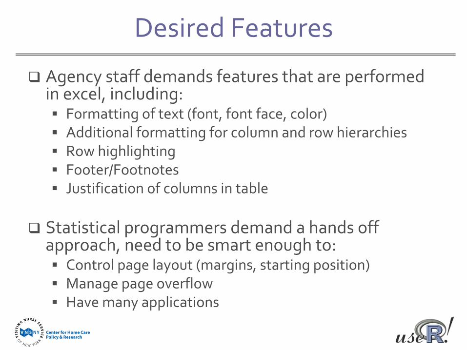
Desired Features

Agency staff demands features that are performed in excel, including: Formatting of text (font, font face, color)  Additional formatting for column and row hierarchies Row highlighting Footer/Footnotes Justification of columns in table

Statistical programmers demand a hands off approach, need to be smart enough to: Control page layout (margins, starting position) Manage page overflow Have many applications

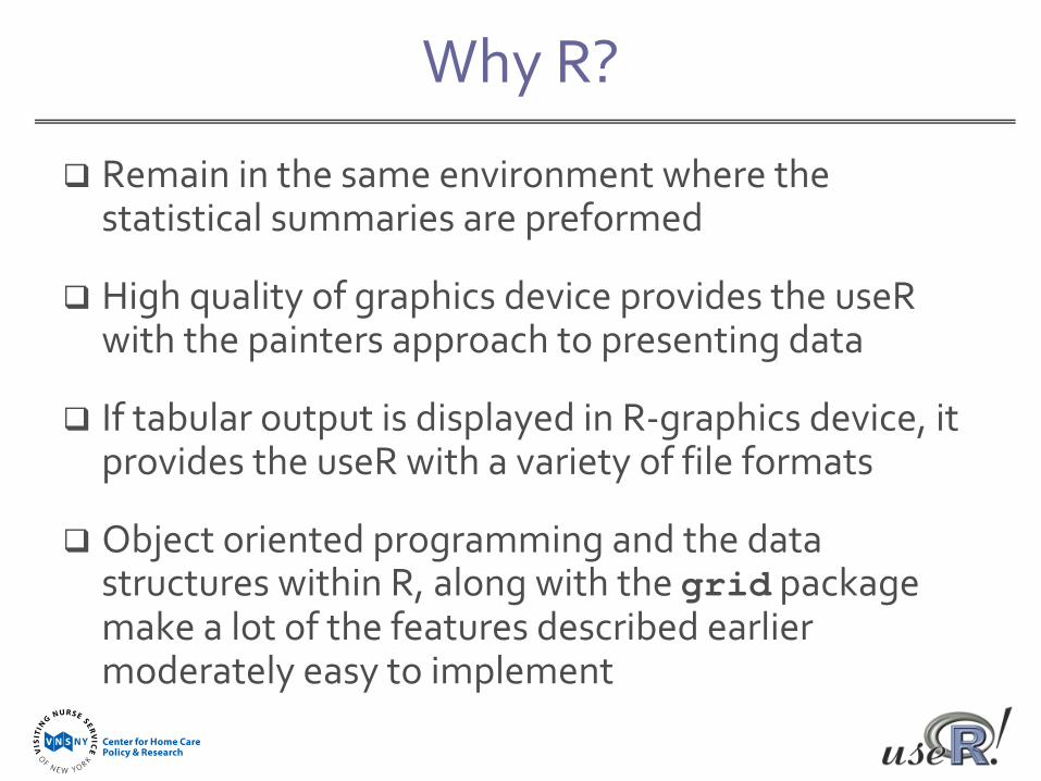
Why R?

Remain in the same environment where the statistical summaries are preformed

High quality of graphics device provides the useRwith the painters approach to presenting data

If tabular output is displayed in R‐graphics device, it provides the useR with a variety of file formats

Object oriented programming and the data structures within R, along with the grid package make a lot of the features described earlier moderately easy to implement

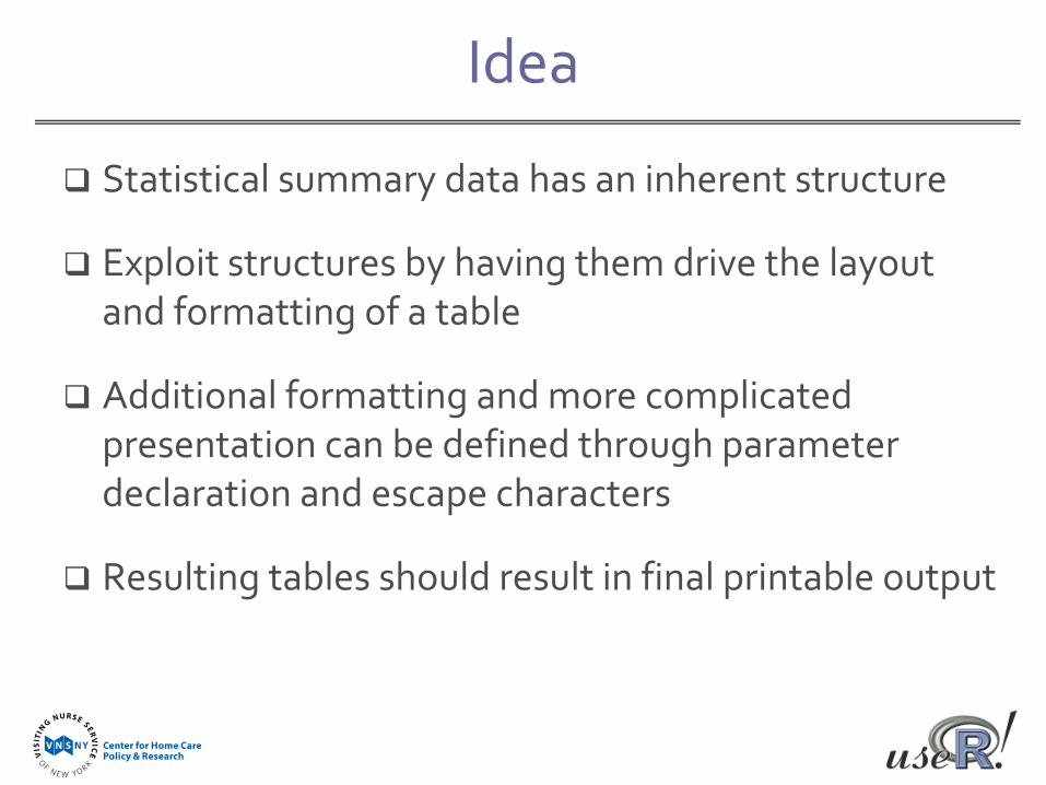
Idea

Statistical summary data has an inherent structure

Exploit structures by having them drive the layout and formatting of a table

Additional formatting and more complicated presentation can be defined through parameter declaration and escape characters

Resulting tables should result in final printable output

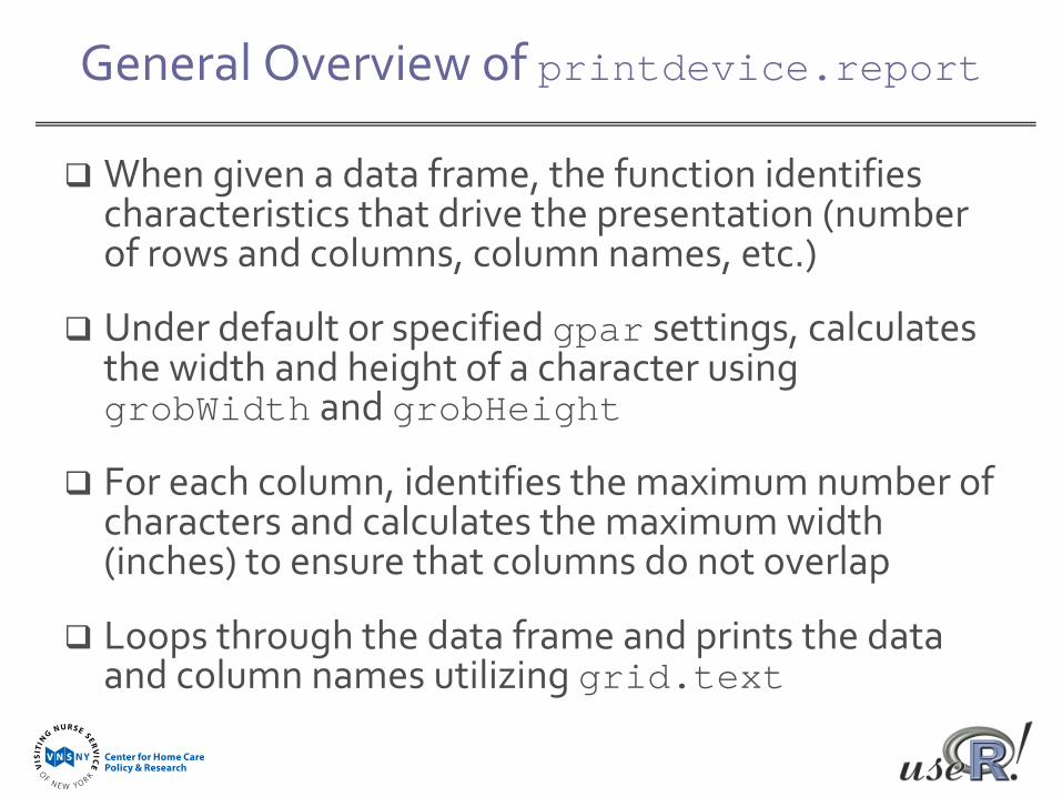
General Overview of printdevice.report

When given a data frame, the function identifies characteristics that drive the presentation (number of rows and columns, column names, etc.)

Under default or specified gpar settings, calculates the width and height of a character using grobWidth and grobHeight

For each column, identifies the maximum number of characters and calculates the maximum width (inches) to ensure that columns do not overlap

Loops through the data frame and prints the data and column names utilizing grid.text

Basic Function Call

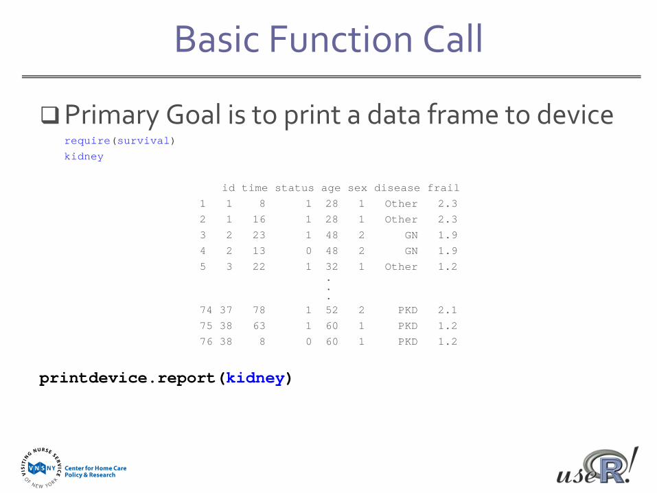
Primary Goal is to print a data frame to devicerequire(survival)kidney

id time status age sex disease frail1 1 8 1 28 1 Other 2.32 1 16 1 28 1 Other 2.33 2 23 1 48 2 GN 1.94 2 13 0 48 2 GN 1.95 3 22 1 32 1 Other 1.2

.

.

.74 37 78 1 52 2 PKD 2.175 38 63 1 60 1 PKD 1.276 38 8 0 60 1 PKD 1.2

printdevice.report(kidney)

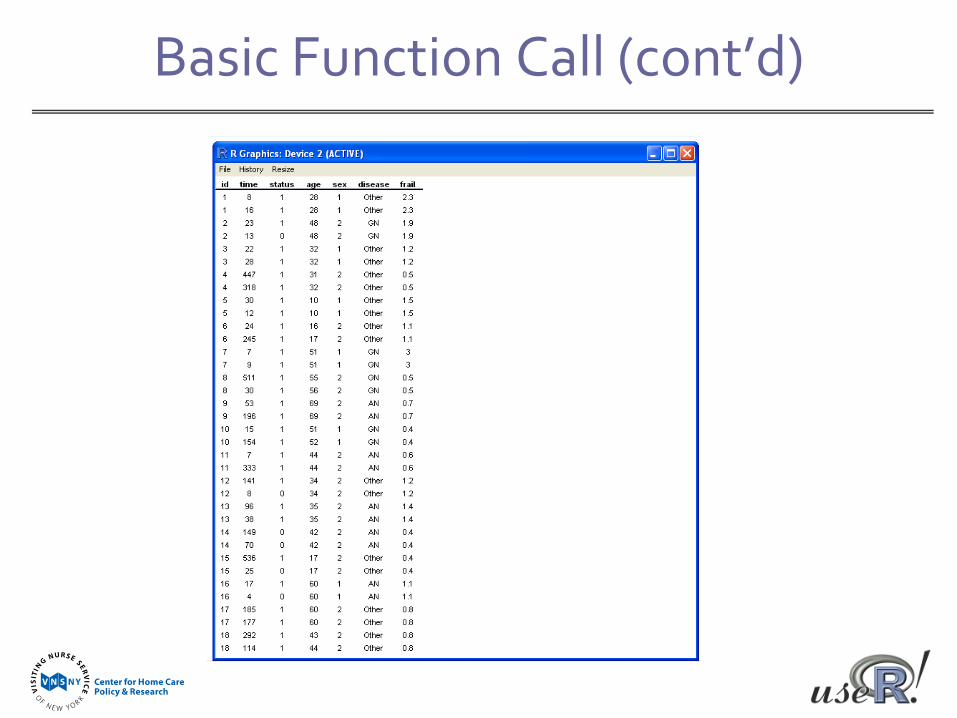
Basic Function Call (cont’d)

Table Row & Column Hierarchies

The presentation of high dimensional summary data requires one to define how to simplify the dimensions in rows and columns while staying within a page layout

This function allows two dimensions of formatting for rows and columns Row dimensions are defined by declaring which column 

names label both dimensions (the “group” and “label”parameter)o Label alone just moves that column all the way to the lefto Group is the higher dimensional description that encompasses the label

Columns of the table can be grouped together by repeating the group name followed by the escape character (“!!!”) in the column names

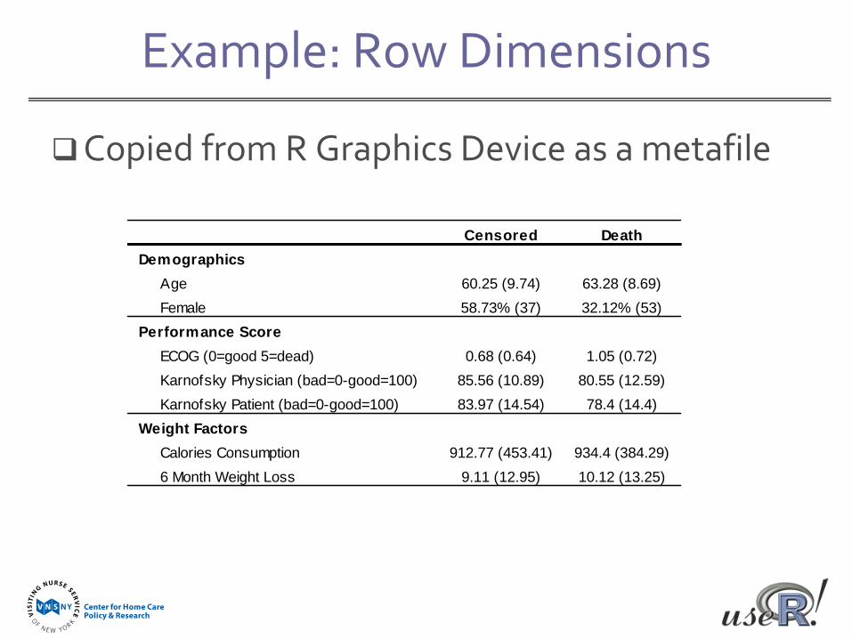
Example: Row Dimensions

Copied from R Graphics Device as a metafile

DemographicsAge 60.25 (9.74) 63.28 (8.69)Female 58.73% (37) 32.12% (53)

Performance ScoreECOG (0=good 5=dead) 0.68 (0.64) 1.05 (0.72)Karnofsky Physician (bad=0-good=100) 85.56 (10.89) 80.55 (12.59)Karnofsky Patient (bad=0-good=100) 83.97 (14.54) 78.4 (14.4)

Weight FactorsCalories Consumption 912.77 (453.41) 934.4 (384.29)6 Month Weight Loss 9.11 (12.95) 10.12 (13.25)

Censored Death

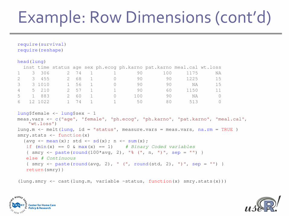
Example: Row Dimensions (cont’d)require(survival)require(reshape)

head(lung)inst time status age sex ph.ecog ph.karno pat.karno meal.cal wt.loss

1 3 306 2 74 1 1 90 100 1175 NA2 3 455 2 68 1 0 90 90 1225 153 3 1010 1 56 1 0 90 90 NA 154 5 210 2 57 1 1 90 60 1150 115 1 883 2 60 1 0 100 90 NA 06 12 1022 1 74 1 1 50 80 513 0

lung$female <- lung$sex - 1meas.vars <- c("age", "female", "ph.ecog", "ph.karno", "pat.karno", "meal.cal",

"wt.loss")lung.m <- melt(lung, id = "status", measure.vars = meas.vars, na.rm = TRUE )smry.stats <- function(x)

{avg <- mean(x); std <- sd(x); n <- sum(x);if (min(x) == 0 & max(x) == 1) # Binary Coded variables{ smry <- paste(round(100*avg, 2), "% (", n, ")", sep = "") }else # Continuous{ smry <- paste(round(avg, 2), " (", round(std, 2), ")", sep = "") }return(smry)}

(lung.smry <- cast(lung.m, variable ~status, function(x) smry.stats(x)))

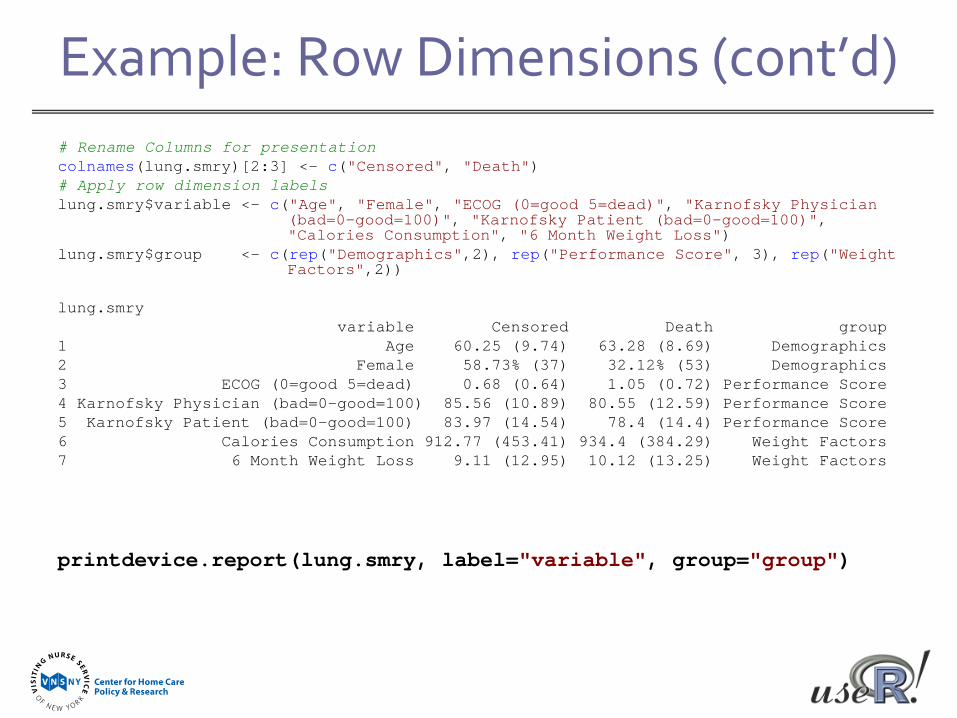
Example: Row Dimensions (cont’d)# Rename Columns for presentationcolnames(lung.smry)[2:3] <- c("Censored", "Death")# Apply row dimension labelslung.smry$variable <- c("Age", "Female", "ECOG (0=good 5=dead)", "Karnofsky Physician

(bad=0-good=100)", "Karnofsky Patient (bad=0-good=100)", "Calories Consumption", "6 Month Weight Loss")

lung.smry$group <- c(rep("Demographics",2), rep("Performance Score", 3), rep("WeightFactors",2))

lung.smryvariable Censored Death group

1 Age 60.25 (9.74) 63.28 (8.69) Demographics2 Female 58.73% (37) 32.12% (53) Demographics3 ECOG (0=good 5=dead) 0.68 (0.64) 1.05 (0.72) Performance Score4 Karnofsky Physician (bad=0-good=100) 85.56 (10.89) 80.55 (12.59) Performance Score5 Karnofsky Patient (bad=0-good=100) 83.97 (14.54) 78.4 (14.4) Performance Score6 Calories Consumption 912.77 (453.41) 934.4 (384.29) Weight Factors7 6 Month Weight Loss 9.11 (12.95) 10.12 (13.25) Weight Factors

printdevice.report(lung.smry, label="variable", group="group")

Example: Column Dimensions

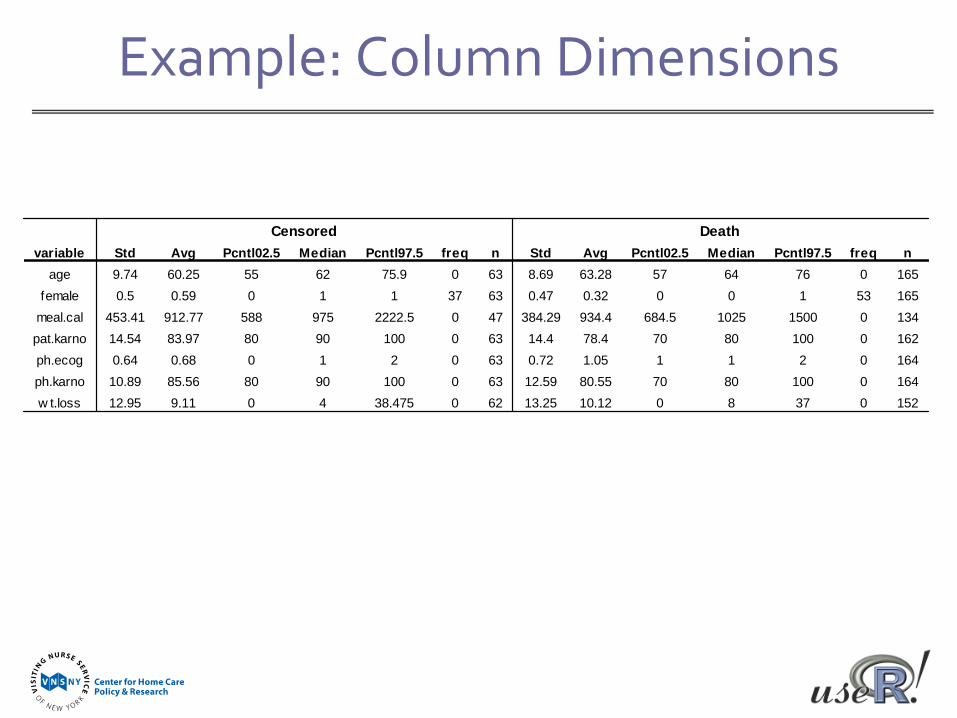
age 9.74 60.25 55 62 75.9 0 63 8.69 63.28 57 64 76 0 165female 0.5 0.59 0 1 1 37 63 0.47 0.32 0 0 1 53 165

meal.cal 453.41 912.77 588 975 2222.5 0 47 384.29 934.4 684.5 1025 1500 0 134pat.karno 14.54 83.97 80 90 100 0 63 14.4 78.4 70 80 100 0 162ph.ecog 0.64 0.68 0 1 2 0 63 0.72 1.05 1 1 2 0 164ph.karno 10.89 85.56 80 90 100 0 63 12.59 80.55 70 80 100 0 164w t.loss 12.95 9.11 0 4 38.475 0 62 13.25 10.12 0 8 37 0 152

variable Std Avg Pcntl02.5 Median Pcntl97.5 freq n Std Avg Pcntl02.5 Median Pcntl97.5 freq nCensored Death

Example: Column Dimensions (cont’d)

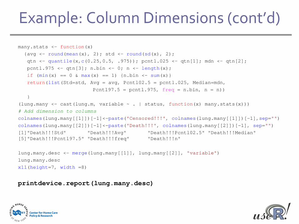
many.stats <- function(x){avg <- round(mean(x), 2); std <- round(sd(x), 2); qtn <- quantile(x,c(0.25,0.5, .975)); pcntl.025 <- qtn[1]; mdn <- qtn[2]; pcntl.975 <- qtn[3]; n.bin <- 0; n <- length(x);if (min(x) == 0 & max(x) == 1) {n.bin <- sum(x)}return(list(Std=std, Avg = avg, Pcntl02.5 = pcntl.025, Median=mdn,

Pcntl97.5 = pcntl.975, freq = n.bin, n = n))}

(lung.many <- cast(lung.m, variable ~ . | status, function(x) many.stats(x)))# Add dimension to columnscolnames(lung.many[[1]])[-1]<-paste("Censored!!!", colnames(lung.many[[1]])[-1],sep="")colnames(lung.many[[2]])[-1]<-paste("Death!!!", colnames(lung.many[[2]])[-1], sep="")[1]"Death!!!Std" "Death!!!Avg" "Death!!!Pcntl02.5" "Death!!!Median" [5]"Death!!!Pcntl97.5" "Death!!!freq" "Death!!!n"

lung.many.desc <- merge(lung.many[[1]], lung.many[[2]], "variable")lung.many.descx11(height=7, width =8)

printdevice.report(lung.many.desc)

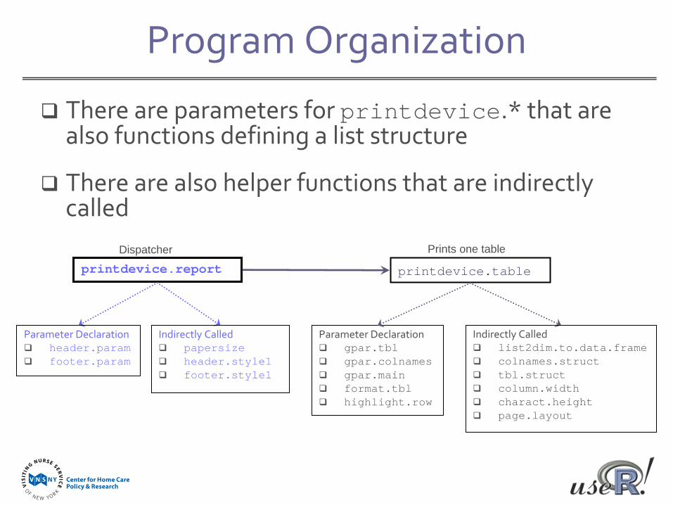
Program Organization

Parameter Declaration gpar.tbl gpar.colnames gpar.main format.tbl highlight.row

printdevice.tableprintdevice.reportDispatcher Prints one table

Indirectly Called list2dim.to.data.frame colnames.struct tbl.struct column.width charact.height page.layout

Parameter Declaration header.param footer.param

Indirectly Called papersize header.style1 footer.style1

There are parameters for printdevice.* that are also functions defining a list structure

There are also helper functions that are indirectly called

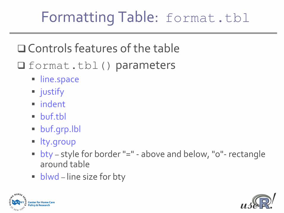
Formatting Table:  format.tbl

Controls features of the table format.tbl() parameters line.space justify indent buf.tbl buf.grp.lbl lty.group bty – style for border "=" ‐ above and below, "o"‐ rectangle 

around table blwd – line size for bty

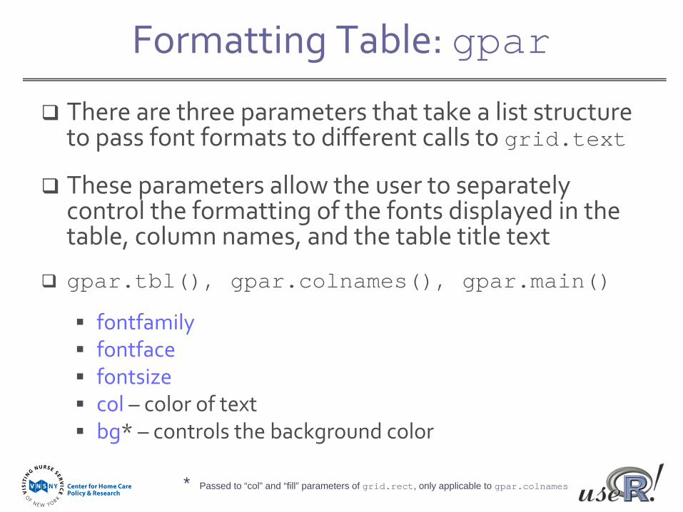
Formatting Table: gpar

There are three parameters that take a list structure to pass font formats to different calls to grid.text

These parameters allow the user to separately control the formatting of the fonts displayed in the table, column names, and the table title text

gpar.tbl(), gpar.colnames(), gpar.main()

fontfamily fontface fontsize col – color of text bg* – controls the background color

* Passed to “col” and “fill” parameters of grid.rect, only applicable to gpar.colnames

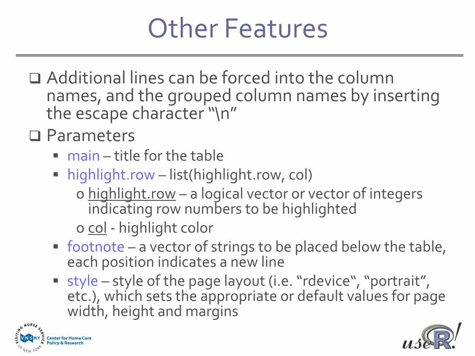
Other Features

Additional lines can be forced into the column names, and the grouped column names by inserting the escape character “\n”

Parameters main – title for the table highlight.row – list(highlight.row, col)

o highlight.row – a logical vector or vector of integers indicating row numbers to be highlighted

o col ‐ highlight color footnote – a vector of strings to be placed below the table, 

each position indicates a new line style – style of the page layout (i.e. “rdevice“, “portrait”, 

etc.), which sets the appropriate or default values for page width, height and margins

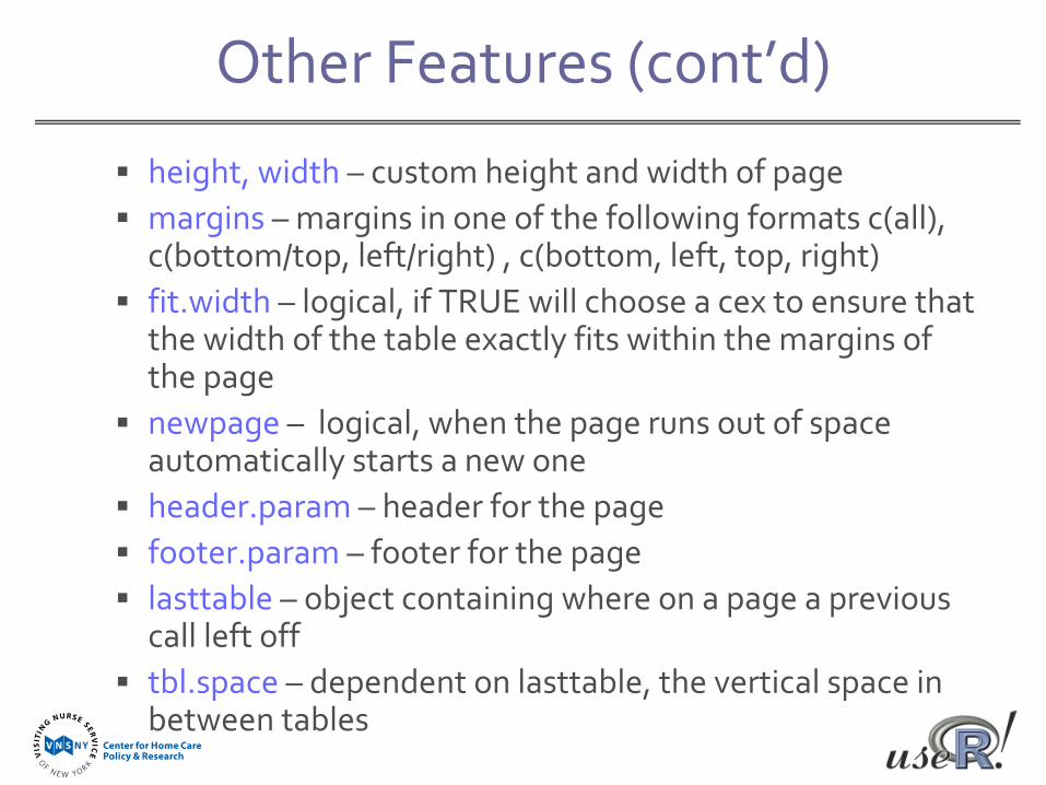
Other Features (cont’d)

height, width – custom height and width of page  margins – margins in one of the following formats c(all), 

c(bottom/top, left/right) , c(bottom, left, top, right) fit.width – logical, if TRUE will choose a cex to ensure that 

the width of the table exactly fits within the margins of the page

newpage – logical, when the page runs out of space automatically starts a new one

header.param – header for the page footer.param – footer for the page lasttable – object containing where on a page a previous 

call left off tbl.space – dependent on lasttable, the vertical space in 

between tables

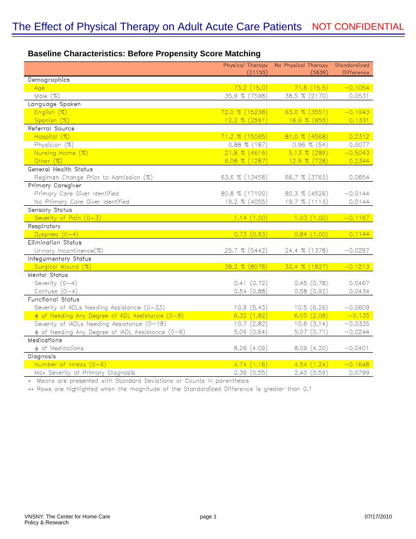
Baseline Characteristics: Before Propensity Score Matching

The Effect of Physical Therapy on Adult Acute Care Patients NOT CONFIDENTIAL

VNSNY: The Center for Home CarePolicy & Research

page 1 07/17/2010

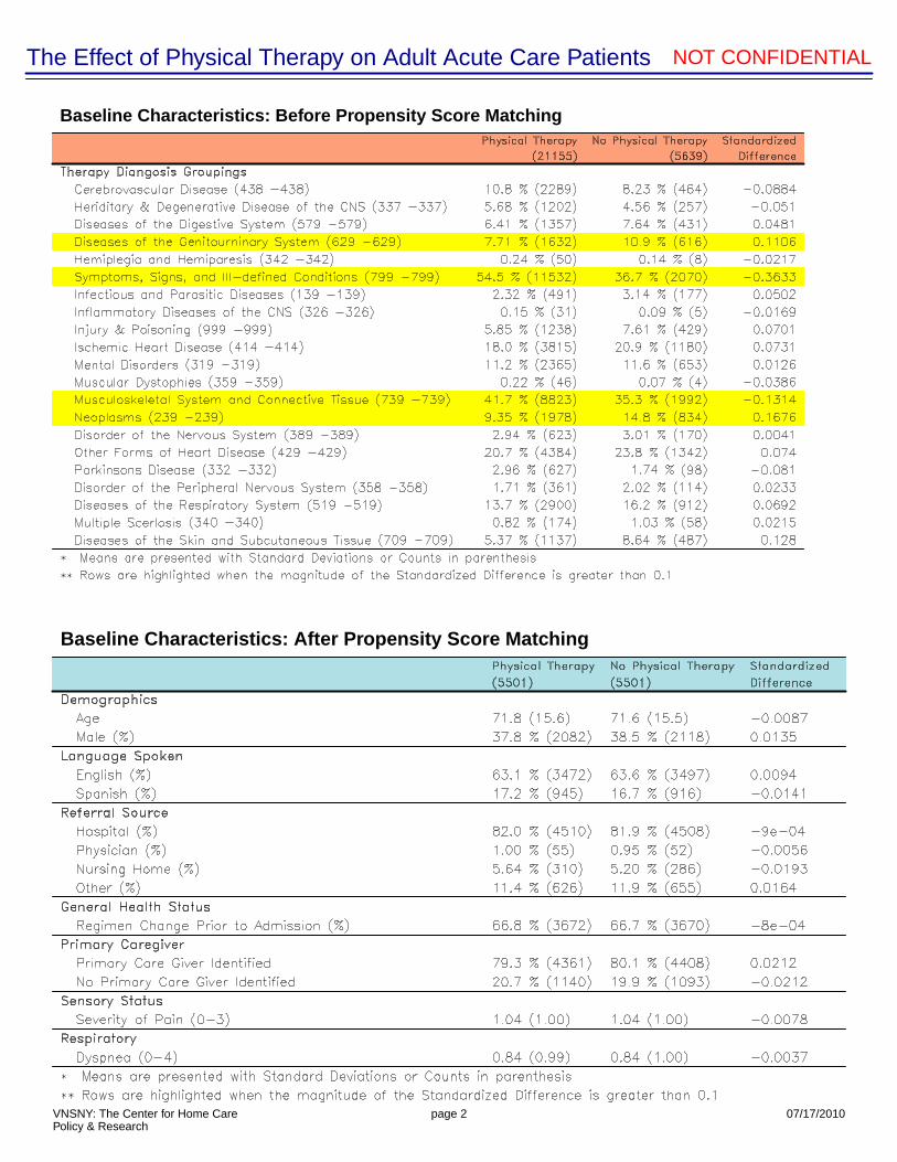
Baseline Characteristics: Before Propensity Score Matching

The Effect of Physical Therapy on Adult Acute Care Patients NOT CONFIDENTIAL

VNSNY: The Center for Home CarePolicy & Research

page 2 07/17/2010

Baseline Characteristics: After Propensity Score Matching

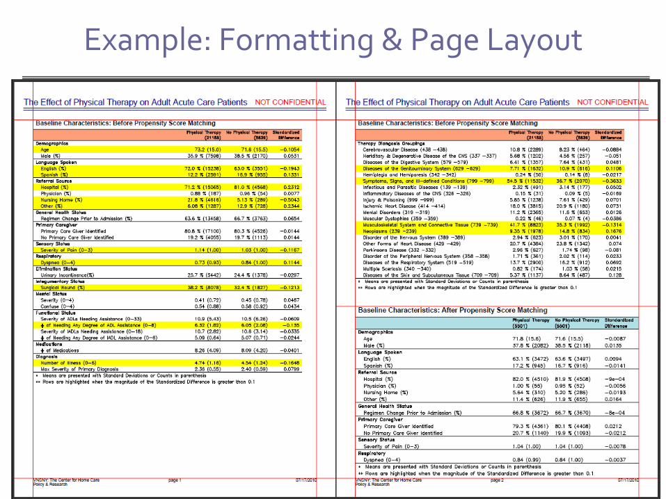
Example: Formatting & Page Layout

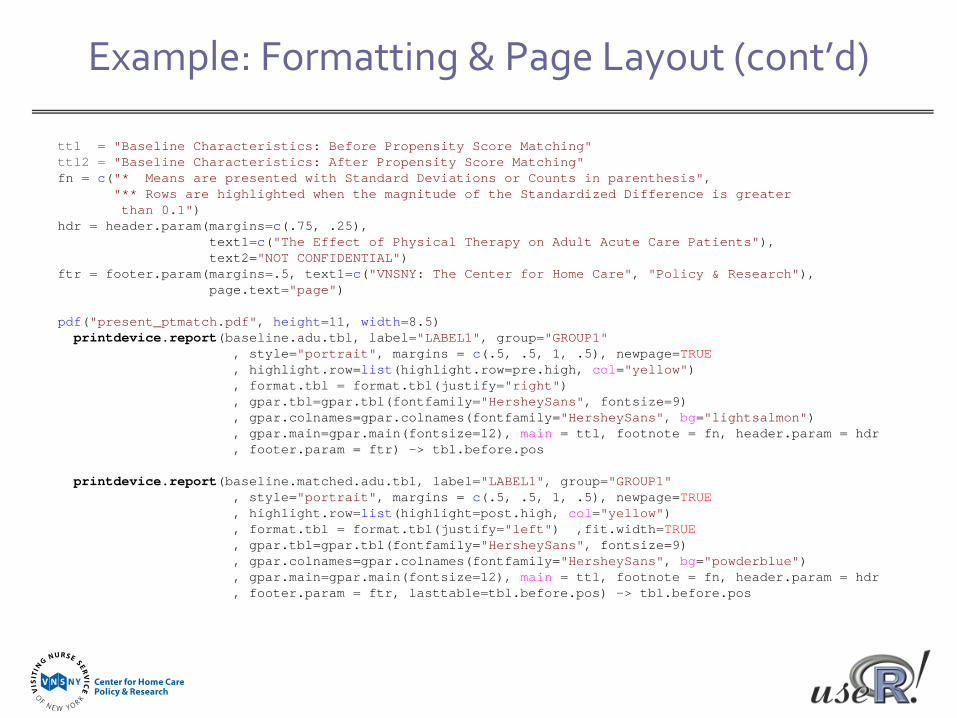
Example: Formatting & Page Layout (cont’d)

ttl = "Baseline Characteristics: Before Propensity Score Matching"ttl2 = "Baseline Characteristics: After Propensity Score Matching"fn = c("* Means are presented with Standard Deviations or Counts in parenthesis",

"** Rows are highlighted when the magnitude of the Standardized Difference is greater than 0.1")

hdr = header.param(margins=c(.75, .25), text1=c("The Effect of Physical Therapy on Adult Acute Care Patients"),text2="NOT CONFIDENTIAL")

ftr = footer.param(margins=.5, text1=c("VNSNY: The Center for Home Care", "Policy & Research"), page.text="page")

pdf("present_ptmatch.pdf", height=11, width=8.5)printdevice.report(baseline.adu.tbl, label="LABEL1", group="GROUP1"

, style="portrait", margins = c(.5, .5, 1, .5), newpage=TRUE, highlight.row=list(highlight.row=pre.high, col="yellow"), format.tbl = format.tbl(justify="right"), gpar.tbl=gpar.tbl(fontfamily="HersheySans", fontsize=9), gpar.colnames=gpar.colnames(fontfamily="HersheySans", bg="lightsalmon") , gpar.main=gpar.main(fontsize=12), main = ttl, footnote = fn, header.param = hdr, footer.param = ftr) -> tbl.before.pos

printdevice.report(baseline.matched.adu.tbl, label="LABEL1", group="GROUP1", style="portrait", margins = c(.5, .5, 1, .5), newpage=TRUE, highlight.row=list(highlight=post.high, col="yellow"), format.tbl = format.tbl(justify="left") ,fit.width=TRUE, gpar.tbl=gpar.tbl(fontfamily="HersheySans", fontsize=9), gpar.colnames=gpar.colnames(fontfamily="HersheySans", bg="powderblue"), gpar.main=gpar.main(fontsize=12), main = ttl, footnote = fn, header.param = hdr, footer.param = ftr, lasttable=tbl.before.pos) -> tbl.before.pos

Baseline

End

Poi

nt

0 5 10 15 20 25

05

1015

2025 Effects:

No PTReceived PT

*

*

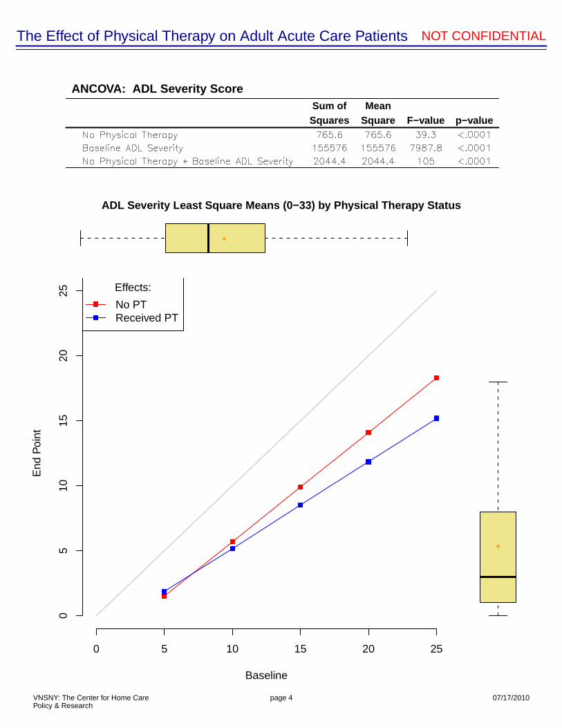
ADL Severity Least Square Means (0−33) by Physical Therapy Status

Sum ofSquares

MeanSquare F−value p−value

ANCOVA: ADL Severity Score

The Effect of Physical Therapy on Adult Acute Care Patients NOT CONFIDENTIAL

VNSNY: The Center for Home CarePolicy & Research

page 4 07/17/2010

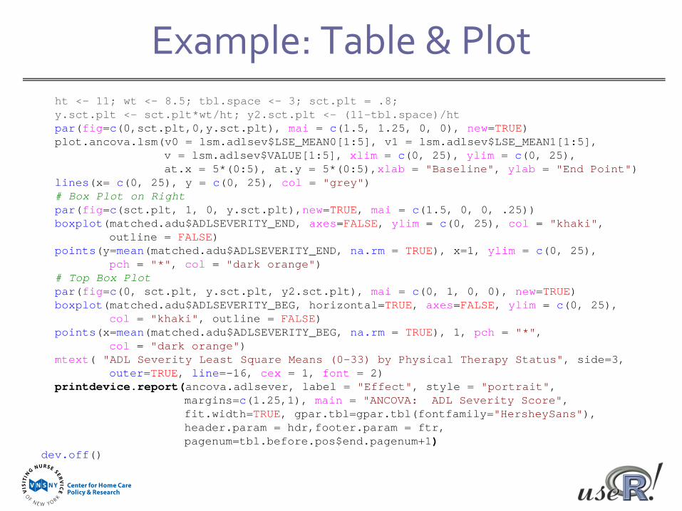
Example: Table & Plotht <- 11; wt <- 8.5; tbl.space <- 3; sct.plt = .8;y.sct.plt <- sct.plt*wt/ht; y2.sct.plt <- (11-tbl.space)/htpar(fig=c(0,sct.plt,0,y.sct.plt), mai = c(1.5, 1.25, 0, 0), new=TRUE)plot.ancova.lsm(v0 = lsm.adlsev$LSE_MEAN0[1:5], v1 = lsm.adlsev$LSE_MEAN1[1:5],

v = lsm.adlsev$VALUE[1:5], xlim = c(0, 25), ylim = c(0, 25),at.x = 5*(0:5), at.y = 5*(0:5),xlab = "Baseline", ylab = "End Point")

lines(x= c(0, 25), y = c(0, 25), col = "grey")# Box Plot on Rightpar(fig=c(sct.plt, 1, 0, y.sct.plt),new=TRUE, mai = c(1.5, 0, 0, .25))boxplot(matched.adu$ADLSEVERITY_END, axes=FALSE, ylim = c(0, 25), col = "khaki",

outline = FALSE)points(y=mean(matched.adu$ADLSEVERITY_END, na.rm = TRUE), x=1, ylim = c(0, 25),

pch = "*", col = "dark orange")# Top Box Plotpar(fig=c(0, sct.plt, y.sct.plt, y2.sct.plt), mai = c(0, 1, 0, 0), new=TRUE)boxplot(matched.adu$ADLSEVERITY_BEG, horizontal=TRUE, axes=FALSE, ylim = c(0, 25),

col = "khaki", outline = FALSE)points(x=mean(matched.adu$ADLSEVERITY_BEG, na.rm = TRUE), 1, pch = "*",

col = "dark orange")mtext( "ADL Severity Least Square Means (0-33) by Physical Therapy Status", side=3,

outer=TRUE, line=-16, cex = 1, font = 2)printdevice.report(ancova.adlsever, label = "Effect", style = "portrait",

margins=c(1.25,1), main = "ANCOVA: ADL Severity Score", fit.width=TRUE, gpar.tbl=gpar.tbl(fontfamily="HersheySans"), header.param = hdr,footer.param = ftr, pagenum=tbl.before.pos$end.pagenum+1)

dev.off()

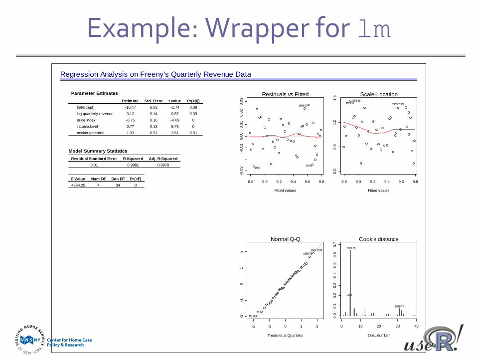
Example: Wrapper for lm

(Intercept) -10.47 6.02 -1.74 0.09lag.quarterly.revenue 0.12 0.14 0.87 0.39price.index -0.75 0.16 -4.69 0income.level 0.77 0.13 5.73 0market.potential 1.33 0.51 2.61 0.01

Estimate Std. Error t value Pr(>|t|)

Parameter Estimates

Regression Analysis on Freeny's Quarterly Revenue Data

0.01 0.9981 0.9978Residual Standard Error R-Squared Adj. R-Squared

Model Summary Statistics

4354.25 4 34 0F Value Num DF Den DF Pr(>F)

8.8 9.0 9.2 9.4 9.6 9.8

-0.0

3-0

.01

0.00

0.01

0.02

0.03

Fitted values

Residuals vs Fitted

1969.75

19631970

-2 -1 0 1 2

-2-1

01

2

Theoretical Quantiles

Normal Q-Q

1963.25

1963

1969.75

8.8 9.0 9.2 9.4 9.6 9.8

0.0

0.5

1.0

1.5

Fitted values

Scale-Location1963.25

1963 1969.75

0 10 20 30 40

0.0

0.1

0.2

0.3

0.4

0.5

0.6

0.7

Obs. number

Cook's distance1963.25

1963

1969.75

Example: Wrapper for lm (cont’d)printdevice.lm( y ~ ., data = freeny, which.plots =1:4, main = "Regression

Analysis on Freeny's Quarterly Revenue Data")

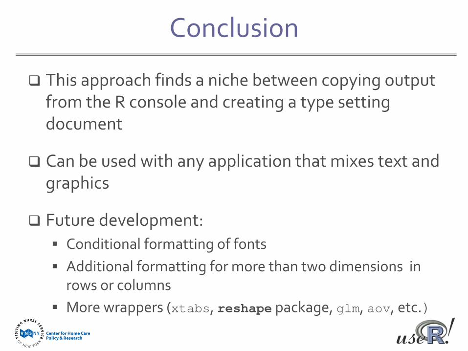
Conclusion

This approach finds a niche between copying output from the R console and creating a type setting document

Can be used with any application that mixes text and graphics

Future development: Conditional formatting of fonts Additional formatting for more than two dimensions  in 

rows or columns More wrappers (xtabs, reshape package, glm, aov, etc.)

Thank You