graphics with maxima - austromath · graphics with maxima (version 5.23 and above) wilhelm haager...

Graphics with MAXIMA(Version 5.23 and above)

Wilhelm HaagerHTL St. Pölten, Department Electrical Engineering

[email protected]

November 26, 2011

Contents ii

Contents

1 Basics 1

2 Gnuplot 32.1 Gnuplot Commands . . . . . . . . . . . . . . . . . . . . . . . . . . . . . . . . . . . . . . . 32.2 Gnuplot Terminals . . . . . . . . . . . . . . . . . . . . . . . . . . . . . . . . . . . . . . . . 42.3 Initialization . . . . . . . . . . . . . . . . . . . . . . . . . . . . . . . . . . . . . . . . . . . . 5

3 Graphic Interface Plot 63.1 Plot Commands . . . . . . . . . . . . . . . . . . . . . . . . . . . . . . . . . . . . . . . . . . 63.2 Options . . . . . . . . . . . . . . . . . . . . . . . . . . . . . . . . . . . . . . . . . . . . . . . 10

4 Graphic Interface Draw 144.1 Plot Commands . . . . . . . . . . . . . . . . . . . . . . . . . . . . . . . . . . . . . . . . . . 144.2 2d-Graphic Objects . . . . . . . . . . . . . . . . . . . . . . . . . . . . . . . . . . . . . . . . 154.3 3d-graphic objects . . . . . . . . . . . . . . . . . . . . . . . . . . . . . . . . . . . . . . . . 194.4 General Options . . . . . . . . . . . . . . . . . . . . . . . . . . . . . . . . . . . . . . . . . 224.5 Options for Labels and Vectors . . . . . . . . . . . . . . . . . . . . . . . . . . . . . . . . 264.6 Options for 2d-Graphics . . . . . . . . . . . . . . . . . . . . . . . . . . . . . . . . . . . . . 274.7 Options for 3d-Graphics . . . . . . . . . . . . . . . . . . . . . . . . . . . . . . . . . . . . . 29

Bibliography 32

1 Basics 1

1 Basics

Maxima uses the program Gnuplot for depicting graphics [2], which is called automatically,when the graphic is produced. Two various methods for displaying the graphics are possible:

1. When calling the standard plotting routines plot2d, plot3d, draw2d, draw3d, etc., a Gnu-plot output window containing the graphic is popping up. Continuing working with Max-ima is not possible until that window is closed again. The Gnuplot output window and

À . . . Graphic in wxMaxima working windowÁ . . . Graphic in Gnuplot output windowÂ . . . Gnuplot console

Wilhelm Haager: Graphics with MAXIMA

1 Basics 2

consequently the graphic too can be resized using the mouse. Measurements can be per-formed in 2d-plots with the mouse, 3d-plots can be rotated in any arbitrary direction.

Right-clicking the window title opens a context menu, which enables printing the graphicand opening the Gnuplot console. Using that console window, Gnuplot can be used as aseparate program, even independently of Maxima.

2. When preceeding the letters “wx” to the names of the plotting routines (wxplot2d,wxplot3d, wxdraw2d, wxdraw3d, . . . ), PNG-graphics are produced in screen resolution andplaced directly into the wxMaxima working window. As the graphics remain visible duringthe entire Maxima session, that method is beneficial for interactive work. Right clickingthe graphic enables copying into the clipboard or saving as a file. Nevertheless, due to itslow resolution, further use of a graphic produced in that way is not reasonable.

Two various Gnuplot interfaces are available, the Maxima standard functions with the stem“plot” in the function names, as well as the routines of the additional package Draw [3] with thestem “draw” in the function names.

The routines of the package Draw are admittedly slightly more complicated concerning theirusage, but they are more flexible than the standard routines and offer much more possibilitiesto adapt the graphics with the aid of options to particular requirements. Furthermore it ispossible, to set output format (eps, png, jpg, etc.) and output target (i. e. the filename) in thegnuplot console after the graphic has been produced, which is appearently not possible whenusing the standard routines of the Gnuplot interface Plot.


2 Gnuplot 3

2 Gnuplot

Gnuplot is a comand-line oriented plot program. When called by Maxima, the input of com-mands into the Gnuplot console window is not necessary in general, but can be helpful, espe-cially when using the Gnuplot interface Draw. For that reason the basic principles and the (few)most inportant commands of Gnuplot are explained below.

2.1 Gnuplot Commands

plotf(x) opts Plotting the function f(x) with the options opts;fundamental command for producing graphics, butthere is no need for it within Maxima.

replot Plotting a graphic anew, occasionally with changedsettings

set terminal term opts Setting the output format, if necessary, with additionaloptions opts.

set output "filename" Setting the output target (filename with theappropriate extension)

set size xscale,yscale Scaling the diagram with respect to the size of theentire grafic

set size ratio n Sets the aspect ratio height/width of the diagram

show item Shows the actual value of item.

cd "directory" Changes the working directory for the output file

pwd Shows the working directory

load "filename" Loads a batch of Gnuplot commands from the filefilename.

set/unset key Turns the lege!ison/off

set/unset hidden3d Turns the visibility of hidden lines in 3d-plots on/off

set/unset grid Turns the coordinate grid on /off

set cntrparam spez Controls contour lines in a contour-plot

set view rotx rotz scale scaley Sets the view point of 3d-plots

quit Exiting Gnuplot; not used within Maxima.

Important Gnuplot Commands

Gnuplot commands are input into the Gnuplot console line by line; one line can contain sev-eral commands, separated by semicolons. Commands and parameters are separated by spaces,particular coordinates by colons. Coordinate ranges have the form [x1:x2].


2 Gnuplot 4

The basic plot command plot is called by Maxima automatically, when a diagram is produced;input of that command by the user does not make sense.

When using the Gnuplot interface Draw, an existing graphic can be drawn anew using thecommand replot, if necessary with changed settings, assigned with the command set andshown with the command show.

set terminal (abbreviated set term) assigns the file format of the produced graphic. A plethoraof formats is available [2], the most important ones are shown in section 2.2 below.

set output assigns the output target, i. e. the name of the graphic file. Unless the entire filepath is given as the parameter, but only the filename, the file is saved in the current workingdirectory (assigned with cd, shown with pwd). The file name stdout causes the graphic to bedrawn into the Gnuplot output window, regardless of the Gnuplot terminal assigned.

The command set output should always be performed after the eventual command set terminal.

The command set size does not assign the size of the entire graphic, but the size of the diagramwithin the graphic with respect to its standard size. Values greater than 1 cause clipping parts ofthe diagram. set size ratio assigns the aspect ratio height/width of the diagram, a negativevalue does not set the ratio of the lengths of the axes, but the ratio of their scales. Thus forexample set size ratio -1 causes the same scale of the x- and y-axis (and not the samelengths); in that case e. g. a circle remains an undistorted cirle.

The command set cntrparam sets the number and values of the contour lines in contour-plotsin various ways:

set cntrparam levels n . . . automatic calculation of n contour linesset cntrparam discrete z1,z2,. . . . . . assigning particular values for contour linesset cntrparam incremental z1,dz,z2 . . . contour lines ranging from z1 to z2 with an

interval of dzset view rotx rotz scale scalez sets the view of 3d-plots. Herein rotx is the rotation around thex-axis (starting from vertical view), rotz the rotation around the z-axis scale a global scale factorand scalez an additional scale factor of the z-axis.

The command load starts batch processing of Gnuplot commands, which are stored in a textfile.

2.2 Gnuplot Terminals

Most Gnuplot terminals offer additional options, which allow adapting the graphic with respectto resolution, size, color depth, font and font size. Unfortunaely the number and the format ofthose options are not coherent for all terminals, in particular the Gnuplot manual or [2] has tobe consulted.


2 Gnuplot 5

Pixel Formats:

dumb retro-style ASCII-art graphic

gif GIF-graphic (suitable for web pages), 8 bit color depth

png Portable Network Graphics, developed in order toreplace GIF, 24 bit color depth

jpeg JPG-graphic

latex LATEX-code with the picture environment

windows on-screen display in the Gnuplot output window

Vector Formats:

aifm Adobe-Illustrator format (file extension .ai)

dxf AutoCAD drawing interchange format

eepic LATEXcode with the extended picture environment(requires the package eepic)

hpgl Hewlett-Packard Graphics Language for pen-plottersand CNC milling machines

postscript Postscript graphic (file extension .ps)

postscript eps Encapsulated Postscript graphic (file extension .eps)

svg Scalable Vector Graphics

Important Gnuplot terminals

2.3 Initialization

gnuplot.ini initialization file for graphic settings

wgnuplot.ini initialization file for Gnuplot settings (i. e. the visualappearance of Gnuplot)

GNUPLOT environment variable, contains the path name of theinitialization files.

Gnuplot-Initialization

Favored standard settings for producing graphics, e. g. the Gnuplot working directory, can beassigned in a file named gnuplot.ini. That file can contain any Gnuplot commands, which areperformed at starting Gnuplot.

Standard settings for the appearance of Gnuplot itself, e. g. text size and window size of thegnuplot console, are assigned in the file wgnuplot.ini. That File is not created by the userdirectly, but via the context menu of of the Gnuplot console.

The directories containing the initialization files gnuplot.ini and wgnuplot.ini are assignedin the environment variable GNUPLOT.


3 Graphic Interface Plot 6

3 Graphic Interface Plot

Plot is the standard Gnuplot interface of Maxima, convenient in its application, but not veryflexible regarding the graphics’ appearance. Furthermore, the possibilities for producing 3d-graphics are very limited. When using this interface, it is unfortunately not possible, to changeappearance, output format or output target of a graphic in the Gnuplot console after the graphichas been drawn.

3.1 Plot Commands

plot2d(f(x),xrange,opts) Plots the function f(x) with the options opts within therange xrange; xrange must be declared.

plot2d([discrete,xwerte,ywerte],opts)Plots the points with declaration of x-values andy-values in two distinct lists xwerte and ywerte; thedeclaration of a range for the x-values is optional.

plot2d([discrete,werte],opts)Other possibility for plotting points; the points aregiven in a nested list [[x1,y1],[x2,y2],...].

plot2d([parametric,x(t),y(t),trange],opts)Plots a parametric curve with the parameter t withinthe range trange

plot3d(f(x,y),xrange,yrange,opts)Plots a function f(x,y) with the options opts within therangs xrange and yrange

plot3d([x(u,v),y(u,v),z(u,v)],urange,vrange,opts)Plots a parametric surface with the parameters u and vwithin the ranges urange and vrange

contour_plot(f(x,y),xrange,yrange,opts)Plots contour lines of a function f(x,y) with the optionsopts within the ranges xrange and yrange

[x,x1,x2] Declaration of a range for the variable x with the lowerbound x1 and the upper bound x2

Plot commands of the Gnuplot interface Plot

The command (wx)plot2d draws a curve or line segments between a couple of points in a two-dimensional cartesian coordinate system. There are three possibilities for that, which can becombined arbitrarily in one single diagram:



1. A function y = f (x); the displayed range along the x-axis must be declared as [x,x1,x2],declaration of y-range is optional.

2. A curve in parametric form x(t), y(t) in dependence of an arbitrarily choosable parametert. If that parameter has actually the name „t“, the declaration of a range can be omitted.In that case t gets the default values as declared with set_plot_option. (the same valuefor all parametric curves) (section 3.2).

3. Particular points, which can be connected (applying the respective options) by line seg-ments. There are two possibilities for the specification of the points: either in two par-ticular lists containing the x-values and the y-values respectively, or in a single nested listcontaining the points, each point representing a list containing its x-value and y-value.

Plotting a function within a declaredrange; the range of the y-axis iscalculated automatically.

(%i1) wxplot2d(sin(x),[x,-%pi,%pi])$

(%t1)

Declaration of x-values in a list: (%i2) xwerte:[0,3,6,4,6,3,0,2,0];

(%o2) [0, 3,6, 4,6, 3,0, 2,0]

Declaration of y-values in a list: (%i3) ywerte:[0,2,0,3,6,4,6,3,0];

(%o3) [0, 2,0, 3,6, 4,6, 3,0]

Two pointwise plots in one diagram withboth ways declaring the points. Thepoints are connected by line segments bydefault.

(%i4) wxplot2d([[discrete,xwerte,ywerte],[discrete,[[3,1],[5,3],[3,5],[1,3],[3,1]]]])$

(%t4)



Curve in paramettic form; in order toachieve a smooth curve, the number ofinitial points has to be increased usingthe option nticks.

(%i5) wxplot2d([parametric,sin(t),sin(2*t),[t,0,2*%pi]],[nticks,100])$

(%t5)

Combination of three vatious 2d-plots inone single diagram; the three respectiveexpressions have to be put into a list.

(%i6) wxplot2d([sin(x),[discrete,xwerte,ywerte],[parametric,10+3*sin(2*t),2+2*cos(3*t),[t,0,2*%pi]]],[x,0,15],[nticks,100])$

(%t6)

One single diagramm can contain any number of curves, put together in a list.

The Gnuplot interface Plot offers only very limited possibilities for creating 3d-plots, they aredescribed below only for the sake of completeness. Anyway, the use of the Gnuplot interfaceDraw is recommended for the creation of 3d-graphics.

Two kinds of 3d-objects can be produced; however, only one single object can be drawn into a3d-graphic:

1. A function z = f (x , y); the ranges for x-values and y-values have to be declared. However,the z-range cannot be declared.

2. An object in parametric form x(u, v), y(u, v), z(u, v) in dependence of two (arbitrarily chooseable)parameters u and v. The ranges of the parameters u and v have to be declared, the rangesof the coordinates x , y and z cannot be declared.



3d-plot of a function in two variables;declaration of the ranges for x and y areoptional, their default values are storedin the list plot_options.

(%i7) wxplot3d(1/(1+x^2+y^2),[x,-3,3],[y,-3,3])$

(%t7)

Parametric form of a surface inthree-dimensional space

(%i8) [fx:cos(x),fy:y,fz:sin(x)+y^2];

(%o8) [cos (x) , y, y2 + sin (x)]

3d-plot of a surface in parametric form (%i9) wxplot3d([fx,fy,fz],[x,0,2*%pi],[y,0,1],[palette,false])$

(%t9)

contour_plot draws contour lines of a function in two variables within the ranges xrangeand yrange, the number and the values of the contour lines can be declared using the optiongnuplot_preamble (sections 2.1 und 3.2).

Contour lines of a function in twovariables. An explicit declaration of thefunction values for the lines, as well asturning off the legend, using theappropriate options, would be benefical.

(%i10) wxcontour_plot(1/(1+x^2+y^2),[x,-3,3],[y,-3,3])$

(%t10)



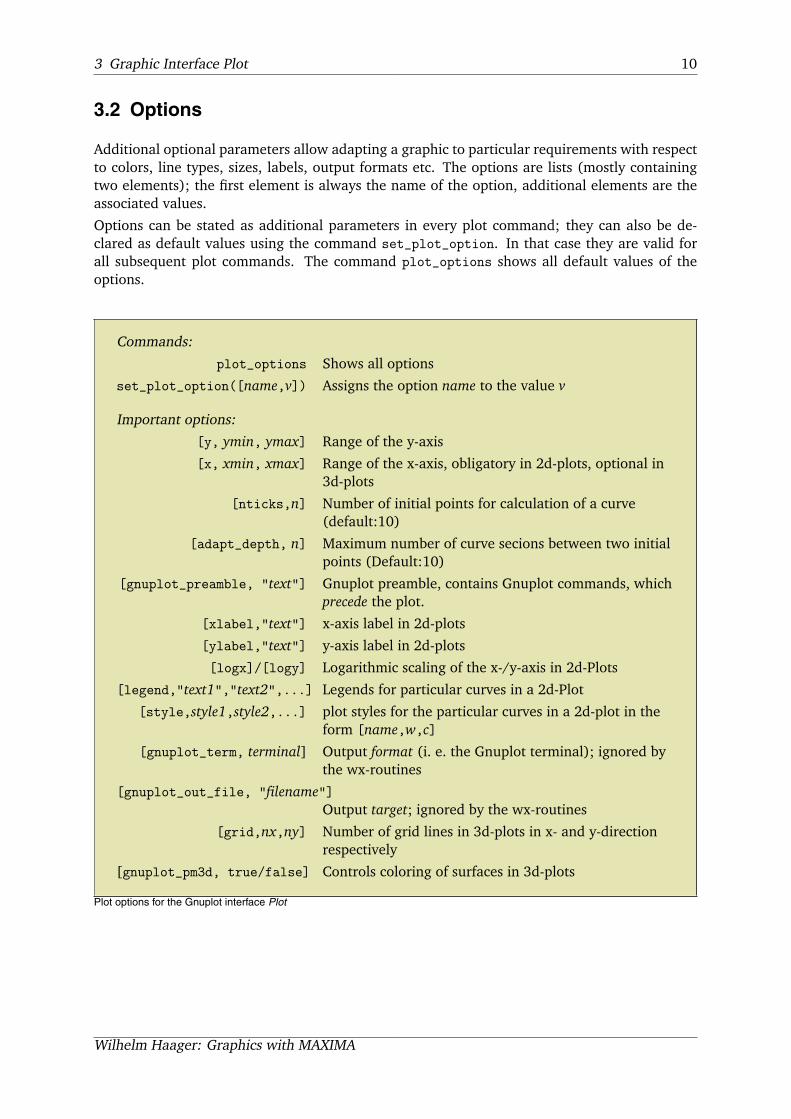
3.2 Options

Additional optional parameters allow adapting a graphic to particular requirements with respectto colors, line types, sizes, labels, output formats etc. The options are lists (mostly containingtwo elements); the first element is always the name of the option, additional elements are theassociated values.

Options can be stated as additional parameters in every plot command; they can also be de-clared as default values using the command set_plot_option. In that case they are valid forall subsequent plot commands. The command plot_options shows all default values of theoptions.

Commands:

plot_options Shows all options

set_plot_option([name,v]) Assigns the option name to the value v

Important options:

[y, ymin, ymax] Range of the y-axis

[x, xmin, xmax] Range of the x-axis, obligatory in 2d-plots, optional in3d-plots

[nticks,n] Number of initial points for calculation of a curve(default:10)

[adapt_depth, n] Maximum number of curve secions between two initialpoints (Default:10)

[gnuplot_preamble, "text"] Gnuplot preamble, contains Gnuplot commands, whichprecede the plot.

[xlabel,"text"] x-axis label in 2d-plots

[ylabel,"text"] y-axis label in 2d-plots

[logx]/[logy] Logarithmic scaling of the x-/y-axis in 2d-Plots

[legend,"text1","text2",...] Legends for particular curves in a 2d-Plot

[style,style1,style2,...] plot styles for the particular curves in a 2d-plot in theform [name,w,c]

[gnuplot_term, terminal] Output format (i. e. the Gnuplot terminal); ignored bythe wx-routines

[gnuplot_out_file, "filename"]Output target; ignored by the wx-routines

[grid,nx,ny] Number of grid lines in 3d-plots in x- and y-directionrespectively

[gnuplot_pm3d, true/false] Controls coloring of surfaces in 3d-plots

Plot options for the Gnuplot interface Plot



The options x and y declare the displayed coordinate ranges, in 2d-plots x is obligatory.

nticks and adapt_depth set the number and maximum division of initial points for calculat-ing the curve. If the displayed curves are sufficiently “smooth”, its explicit declaration is notnecessary.

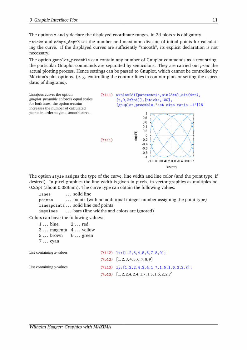
The option gnuplot_preamble can contain any number of Gnuplot commands as a text string,the particular Gnuplot commands are separated by semicolons. They are carried out prior theactual plotting process. Hence settings can be passed to Gnuplot, which cannot be controlled byMaxima’s plot options. (e. g. controlling the contour lines in contour plots or setting the aspectdatio of diagrams).

Lissajous curve; the optiongnuplot_preamble enforces equal scalesfor both axes, the option nticksincreases the number of calculatedpoints in order to get a smooth curve.

(%i11) wxplot2d([parametric,sin(3*t),sin(4*t),[t,0,2*%pi]],[nticks,100],[gnuplot_preamble,"set size ratio -1"])$

(%t11)

The option style assigns the type of the curve, line width and line color (and the point type, ifdesired). In pixel graphics the line width is given in pixels, in vector graphics as multiples od0.25pt (about 0.088mm). The curve type can obtain the following values:

lines . . . solid linepoints . . . points (with an additional integer number assigning the point type)linespoints . . . solid line and pointsimpulses . . . bars (line widths and colors are ignored)

Colors can have the following values:1 . . . blue 2 . . . red3 . . . magenta 4 . . . yellow5 . . . brown 6 . . . green7 . . . cyan

List containing x-values (%i12) lx:[1,2,3,4,5,6,7,8,9];

(%o12) [1, 2,3, 4,5, 6,7, 8,9]

List containing y-values (%i13) ly:[1,2,2.4,2.4,1.7,1.5,1.6,2,2.7];

(%o13) [1, 2,2.4, 2.4,1.7, 1.5,1.6, 2,2.7]



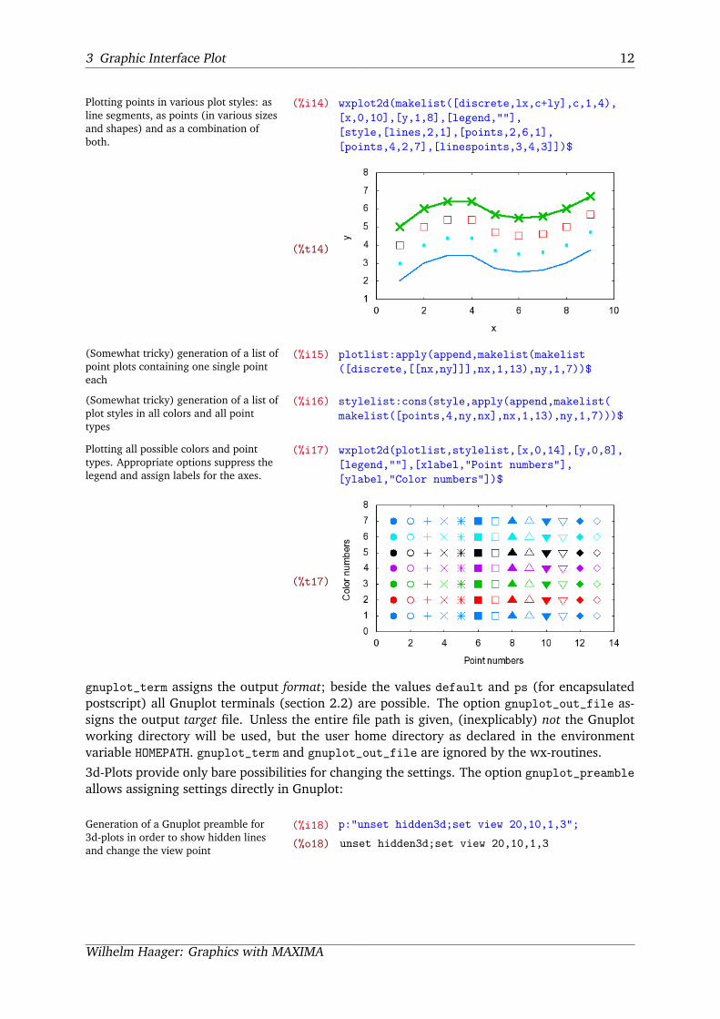
Plotting points in various plot styles: asline segments, as points (in various sizesand shapes) and as a combination ofboth.

(%i14) wxplot2d(makelist([discrete,lx,c+ly],c,1,4),[x,0,10],[y,1,8],[legend,""],[style,[lines,2,1],[points,2,6,1],[points,4,2,7],[linespoints,3,4,3]])$

(%t14)

(Somewhat tricky) generation of a list ofpoint plots containing one single pointeach

(%i15) plotlist:apply(append,makelist(makelist([discrete,[[nx,ny]]],nx,1,13),ny,1,7))$

(Somewhat tricky) generation of a list ofplot styles in all colors and all pointtypes

(%i16) stylelist:cons(style,apply(append,makelist(makelist([points,4,ny,nx],nx,1,13),ny,1,7)))$

Plotting all possible colors and pointtypes. Appropriate options suppress thelegend and assign labels for the axes.

(%i17) wxplot2d(plotlist,stylelist,[x,0,14],[y,0,8],[legend,""],[xlabel,"Point numbers"],[ylabel,"Color numbers"])$

(%t17)

gnuplot_term assigns the output format; beside the values default and ps (for encapsulatedpostscript) all Gnuplot terminals (section 2.2) are possible. The option gnuplot_out_file as-signs the output target file. Unless the entire file path is given, (inexplicably) not the Gnuplotworking directory will be used, but the user home directory as declared in the environmentvariable HOMEPATH. gnuplot_term and gnuplot_out_file are ignored by the wx-routines.

3d-Plots provide only bare possibilities for changing the settings. The option gnuplot_preambleallows assigning settings directly in Gnuplot:

Generation of a Gnuplot preamble for3d-plots in order to show hidden linesand change the view point

(%i18) p:"unset hidden3d;set view 20,10,1,3";

(%o18) unset hidden3d;set view 20,10,1,3



3d-plot with a Gnuplot preamble,changes number of grid lines andturned-off color palette

(%i19) wxplot3d(1/(1+x^2+y^2),[x,-3,3],[y,-3,3],[grid,60,60],[gnuplot_preamble, p],[palette,false])$

(%t19)


4 Graphic Interface Draw 14

4 Graphic Interface Draw

The Gnuplot interface Draw by Mario Rodríguez Riotorto [3] provides an additional set of Max-ima graphic routines, which differ from the standard routines with regard to their parameters,in particular the structure of the options.

The application of these routines, all having the stem “draw” in their function names, is slightlymore complicated than of the standard routines. However, they offer much more flexibility forconfiguration and adapting the graphics to particular requirements. Moreover, output formatand output target can be assigned after the graphic has been drawn into the Gnuplot outputwindow.

The package Draw has to be loaded prior to its first use.

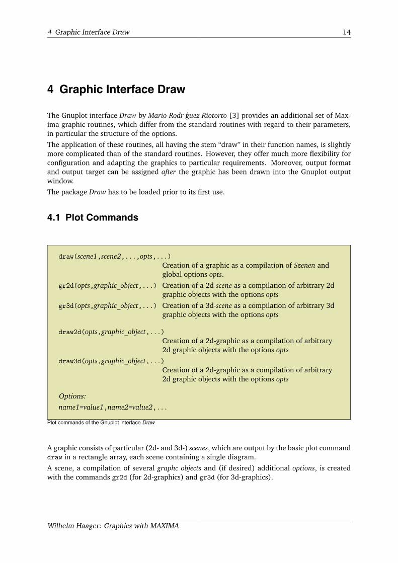
4.1 Plot Commands

draw(scene1,scene2,...,opts,...)Creation of a graphic as a compilation of Szenen andglobal options opts.

gr2d(opts,graphic_object,...) Creation of a 2d-scene as a compilation of arbitrary 2dgraphic objects with the options opts

gr3d(opts,graphic_object,...) Creation of a 3d-scene as a compilation of arbitrary 3dgraphic objects with the options opts

draw2d(opts,graphic_object,...)Creation of a 2d-graphic as a compilation of arbitrary2d graphic objects with the options opts

draw3d(opts,graphic_object,...)Creation of a 2d-graphic as a compilation of arbitrary2d graphic objects with the options opts

Options:

name1=value1,name2=value2,...

Plot commands of the Gnuplot interface Draw

A graphic consists of particular (2d- and 3d-) scenes, which are output by the basic plot commanddraw in a rectangle array, each scene containing a single diagram.

A scene, a compilation of several graphc objects and (if desired) additional options, is createdwith the commands gr2d (for 2d-graphics) and gr3d (for 3d-graphics).



Most graphic contain only one single diagram (i. e. only one single scene). In that case the plotcommands draw2d and draw3d compile the graphic objects to a scene and draw the graphic forthat scene in one single step. Thus The commands

draw2d(...) and draw3d(...)

are equal to

draw(gr2d(...)) and draw(gr3d(...)).

The parameter list contains any number of graphic objects and options. Options referring to aparticular graphic object must precede that object. The position of global parameters (e. g. fordeclaring output format and output target) is arbitrary.

Options are declared as equations with its name on the left hand side and its value on the righthand side. The value can also be a list (e. g. for assigning ranges with lower bound and upperbound).

At complex graphics containing many objects, the parameter list can get long and somewhatconfusing. In that case it is good style, either

• to structure the input by appropriate line breaks and indentations, or (even better)

• not to declare the graphic objects directly in the parameter list of the plot commands, butassign variable names to them in separate commands and use those variable names in theparameter list of the plot commands.

4.2 2d-Graphic Objects

explicit, parametric and implicit create graphic objects from mathematical expressions incartesian coordinates. polar creates a graphic object of a function in polar coordinates. As thedisplayed ranges are an inherent part of the graphic objets, they need not be declared—contraryto the Gnuplot interface Plot—as options.

Furthermore, a number of geometric shapes is available, which allow the composition of ar-bitrary graphics. The graphic object points primarily displays a number of discrete points.Applying the approptiate options, those points can be connected by line segments. Thus pointsenables the creation of any graphic consisting of lines and approximate curves (section 4.4).



explicit(f(x),x,x1,x2) Function f(x) within the range of x1 and x2parametric(x(t),y(t),t,t1,t2)

Parametric curve x(t),y(t) with the parameter t rangingfrom t1 to t2

implicit(equation,x,x1,x2,y,y1,y2)Implicit curve, declared by the equation equation, withthe variables x and y within the ranges x1. . . x2 andy1. . . y2

polar(r(ϕ),ϕ,ϕ1,ϕ2) Function in polar coordinates; radius r with respect tothe angle ϕ in degree ranging from ϕ1 to ϕ2

points(xvals,yvals) Points; xvals and yvals are lists containing the x- andy-values respectively

points(p1,p2,...) Points; each ponint pi is a list with its coordinates:[px,py].

polygon(xvals,yvals) Polygon with declaration of its vertexes in lists xvalsand yvals.

polygon(p1,p2,...) Polygon; each vertex pi is a list containing itscoordinates: [px,py].

rectangle(p1,p2) Rectangle with the opposite vertexes p1 and p2 in theform [px,py]

ellipse(x0,y0,a,b,w1,w2) Ellipse (oder circle) with the center [x0,y0], thehalf-axes a and b, as well as starting angle w1 and finalangle w2

label(["text",x,y],...) Label text at the position [x,y]; alignment andorientation can be set using options.

vector([x,y],[dx,dy]) Vector with the origin [x,y] and the coordinates [dx,dy]

image(m,x,y,nx,ny) Image object with the matrix m containing nx×nxpixels and the coordinates [x,y] of the lower left corner

2d graphic objects

Loading the package Draw (%i20) load(draw);

(%o20) C:/Programme/Maxima-5.23.2/share/maxima/...

Declaring a function y= f (x) as agraphic object

(%i21) g1:explicit(2*sin(x),x,-%pi,%pi);

(%o21) explicit (2 sin (x) , x ,−π,π)

Parametric curve as graphic object (%i22) g2:parametric(2*sin(phi),2*cos(phi),phi,0,2*%pi);

(%o22) parametric�

2sin�

ϕ�

, 2 cos�

ϕ�

,ϕ, 0, 2π�

Implicit function as graphic object (%i23) g3:implicit(x^2-y^2=1,x,-4,4,y,-4,4);

(%o23) implicit�

x2 − y2 = 1, x ,−4,4, y,−4, 4�

Function r= f (ϕ) in polar coordinates asgraphic object

(%i24) g4:polar(1+0.8*sin(13*t),t,0,2*%pi);

(%o24) polar (0.8 sin (13 t) + 1, t, 0, 2π)



Plot all graphic objects into one singlediagram; using the appropriate options,smooth curves are obtained and thediagramm gets some color.

(%i25) wxdraw2d(nticks=200,color=red,g1,color=blue,g2,color=green,g3,color=orange,g4)$

(%t25)

Polygon as graphic object from listscontaining the x-values and y-valueseach

(%i26) poly:polygon(xwerte+2,ywerte+2);

(%o26) polygon ([2,5, 8, 6,8, 5,2, 4,2], [2, 4,2, 5,8, 6,8, 5,2])

“Points”-object from lists containing thex-values and y-values each

(%i27) punkte:points([1,3,5,7,9,9,9,9,9,7,5,3,1,1,1,1],[1,1,1,1,1,3,5,7,9,9,9,9,9,7,5,3]);

(%o27) points ([1, 3,5, 7,9, 9,9, 9,9, 7,5, 3,1, 1,1, 1],[1,1, 1, 1,1, 3,5, 7,9, 9,9, 9,9, 7,5, 3])

Declaring a rectangle by its oppositevertexes

(%i28) rechteck:rectangle([1,-2],[6,-7]);

(%o28) rectangle ([1,−2], [6,−7])

Ellipse as graphic object (%i29) ell:ellipse(6,-6,3,2,0,360);

(%o29) ellipse (6,−6, 3,2, 0,360)

Bar chart as graphic object (%i30) balken:bars([-7,2,1],[-5,5,1],[-3,7,1],[-1,6,1]);

(%o30) bars ([−7, 2,1], [−5, 5,1], [−3, 7,1], [−1,6, 1])

Three vectors as graphic objects (%i31) [v1,v2,v3]:[vector([-8,-8],[6,0]),vector([-8,-8],[6,6]),vector([-2,-8],[0,6])];

(%o31) [vector ([−8,−8], [6,0]) , vector ([−8,−8], [6,6]) ,vector ([−2,−8], [0, 6])]

Textstrings as graphic object “label”; alltexts are put together in one singleobject.

(%i32) text:label(["Bars",-5,-1],["Points and Polygon",5,-1],["Vectors",-5,-9],["Rectangle and Ellipse",5,-9]);

(%o32) label([Bars,−5,−1], [Points and Polygon, 5,−1],[Vectors,−5,−9], [Rectangle and Ellipse, 5,−9])



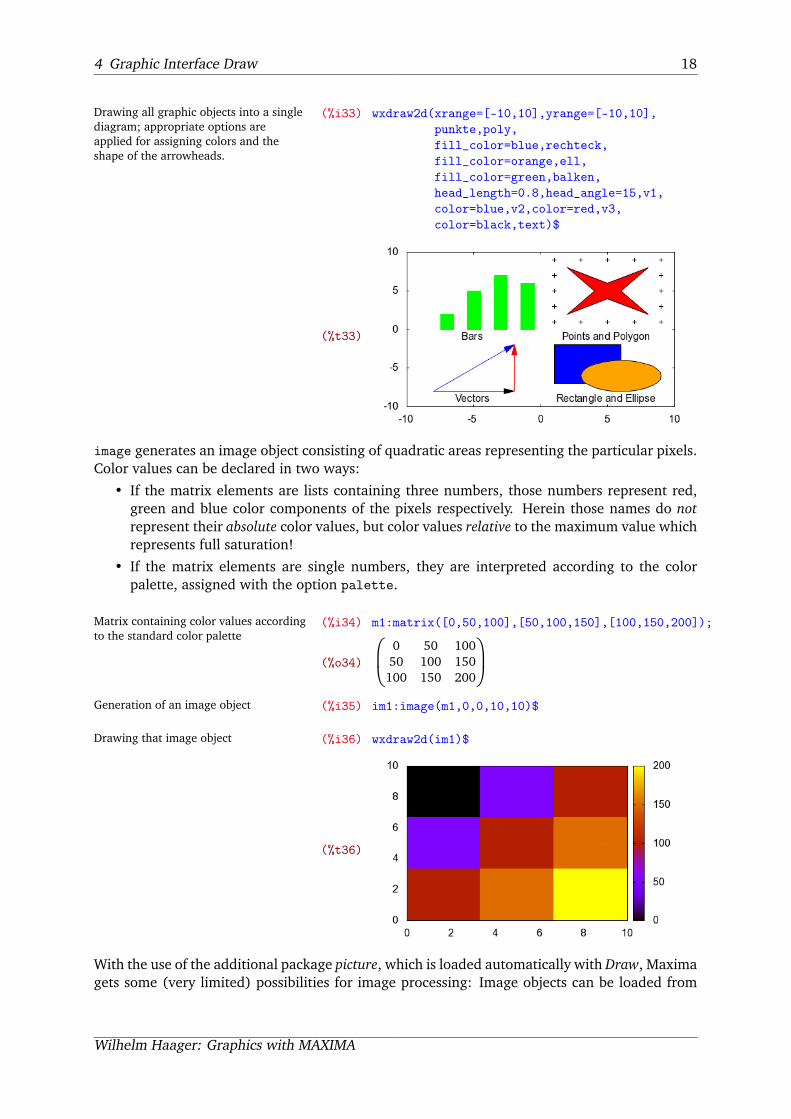
Drawing all graphic objects into a singlediagram; appropriate options areapplied for assigning colors and theshape of the arrowheads.

(%i33) wxdraw2d(xrange=[-10,10],yrange=[-10,10],punkte,poly,fill_color=blue,rechteck,fill_color=orange,ell,fill_color=green,balken,head_length=0.8,head_angle=15,v1,color=blue,v2,color=red,v3,color=black,text)$

(%t33)

image generates an image object consisting of quadratic areas representing the particular pixels.Color values can be declared in two ways:

• If the matrix elements are lists containing three numbers, those numbers represent red,green and blue color components of the pixels respectively. Herein those names do notrepresent their absolute color values, but color values relative to the maximum value whichrepresents full saturation!

• If the matrix elements are single numbers, they are interpreted according to the colorpalette, assigned with the option palette.

Matrix containing color values accordingto the standard color palette

(%i34) m1:matrix([0,50,100],[50,100,150],[100,150,200]);

(%o34)

0 50 10050 100 150

100 150 200

Generation of an image object (%i35) im1:image(m1,0,0,10,10)$

Drawing that image object (%i36) wxdraw2d(im1)$

(%t36)

With the use of the additional package picture, which is loaded automatically with Draw, Maximagets some (very limited) possibilities for image processing: Image objects can be loaded from



XPM-files, color channels can be extracted from images, images can be composed from colorchannels [1], [3].

4.3 3d-graphic objects

explicit(f(x,y),x,x1,x2,y,y1,y2)Function f(x,y) within the ranges x1. . . x2 and y1. . . y2

implicit(equation,x,x1,x2,y,y1,y2,z,z1,z2)Implizit curve defined by equation, in the variables x, yand z within the ranges x1. . . x2, y1. . . y2, z1. . . z2

parametric(x(t),y(t),z(t),t,t1,t2)

Parametric curve x(t),y(t),z(t) with the parameter tranging from t1 to t2

parametric_surface(x(u,v),y(u,v),z(u,v),u,u1,u2,v,v1,v2)Parametric surface x(u,v),y(u,v),z(u,v) with theparameters u and v within the ranges u1. . . u2 andv1. . . v2

cylindrical(r(z,ϕ),z,z1,z2,ϕ,ϕ1,ϕ2)Surface in zylindric coordinates; radius r(z,ϕ) withrespect to the z-coordinate z ranging from z1 to z2 andazimuth ϕ ranging from ϕ1 to ϕ2

spherical(r(ϕ,ϑ),ϕ,ϕ1,ϕ2,ϑ,ϑ1,ϑ2)Surface in spherical coordinates; radius r(ϕ,ϑ) withrespect to the azimuth ϕ ranging from ϕ1 to ϕ2 andthe zenith ϑ ranging from ϑ1 to ϑ2

points(xvals,yvals,zvals) Points; xvals, yvals and zvals are lists containing the x-,y- and z-values respectively

points(p1,p2,...) Points; each point pi is a list containing its coordinates:[px,py,pz].

label(["text",x,y,z],...) Text label text at the position [x,y,z]; alignment, fontetc. can be set using options.

vector([x,y,z],[dx,dy,dz]) Vector with the origin [x,y,z] and its coordinates[dx,dy,dz]

3d-graphic objects

explicit and implicit define graphic objects by mathematical expressions in cartesian coor-dinates as surfaces in three-dimensional space. parametric defines a parametric curve withthe parameter t, parametric_surface defines a surface in parametric form with two parame-ters u and v. cylindrical and spherical define a surface in cylindric and spheric coordinatesrespectively.

Contrary to the Gnuplot interface Plot, one single diagramm can contain any number of graphicobjects.



Sphere, defined as an implicit function (%i37) gimp:implicit(1=x**2+y**2+z**2,x,-1,1,y,-1,1,z,-1,1);

(%o37) implicit�

1= z2 + y2 + x2, x ,−1, 1, y,−1,1, z,−1,1�

Two-dimensional function (%i38) gexp:explicit(sin(2*x)*sin(2*y),x,-2,2,y,-2,2);

(%o38) explicit�

sin (2 x) sin�

2 y�

, x ,−2,2, y,−2, 2�

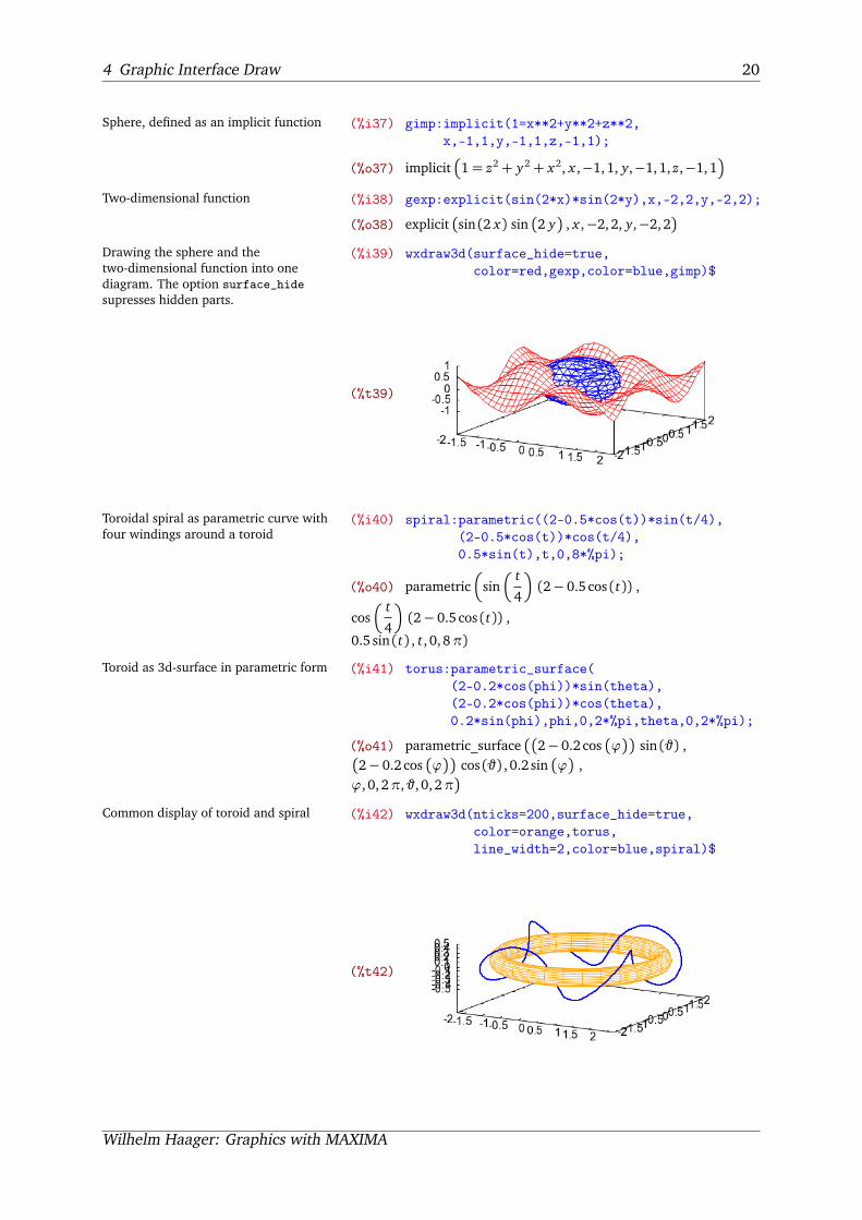
Drawing the sphere and thetwo-dimensional function into onediagram. The option surface_hidesupresses hidden parts.

(%i39) wxdraw3d(surface_hide=true,color=red,gexp,color=blue,gimp)$

(%t39)

Toroidal spiral as parametric curve withfour windings around a toroid

(%i40) spiral:parametric((2-0.5*cos(t))*sin(t/4),(2-0.5*cos(t))*cos(t/4),0.5*sin(t),t,0,8*%pi);

(%o40) parametric�

sin� t

4

�

(2− 0.5cos (t)) ,

cos� t

4

�

(2− 0.5cos (t)) ,

0.5 sin (t) , t, 0, 8π)

Toroid as 3d-surface in parametric form (%i41) torus:parametric_surface((2-0.2*cos(phi))*sin(theta),(2-0.2*cos(phi))*cos(theta),0.2*sin(phi),phi,0,2*%pi,theta,0,2*%pi);

(%o41) parametric_surface��

2− 0.2 cos�

ϕ��

sin (ϑ) ,�

2− 0.2 cos�

ϕ��

cos (ϑ) , 0.2 sin�

ϕ�

,ϕ, 0, 2π,ϑ, 0, 2π

�

Common display of toroid and spiral (%i42) wxdraw3d(nticks=200,surface_hide=true,color=orange,torus,line_width=2,color=blue,spiral)$

(%t42)



Cone as a function in cylindriccoordinates

(%i43) cone:cylindrical((z-15)*0.05,z,-15,15,phi,0,2*%pi);

(%o43) cylindrical�

0.05 (z− 15) , z,−15, 15,ϕ, 0, 2π�

Snail shell like surface, defined inspheric coordinates

(%i44) snail:spherical(4+0.5*phi,phi,-2*%pi,%pi,tht,0,%pi);

(%o44) spherical�

0.5ϕ+ 4,ϕ,−2π,π, tht, 0,π�

Common display of cone and snail shell (%i45) wxdraw3d(surface_hide=true,color=green,cone,color=brown,snail)$

(%t45)

3d-points in the xy-plane, shaping acircle

(%i46) pts:points(makelist([sin(t*%pi/10),cos(t*%pi/10),0],t,1,20))$

Four vectors, forming a compass rose (%i47) [v1,v2,v3,v4]:[vector([0,0,1],[0.7,0,0]),vector([0,0,1],[0,0.7,0]),vector([0,0,1],[-0.7,0,0]),vector([0,0,1],[0,-0.7,0])];

(%o47) [vector ([0, 0,1], [0.7, 0,0]) , vector ([0,0, 1], [0, 0.7,0]) ,vector ([0, 0,1], [−0.7, 0,0]) , vector ([0, 0,1], [0,−0.7, 0])]

Texts in three-dimensional space; thetext is not aligned to the axes, but to theview direction.

(%i48) text:label(["North",0,1,1],["East",1,0,1],["South",0,-1,1],["West",-1,0,1]);

(%o48) label ([Nor th, 0, 1, 1], [East, 1, 0, 1], [South, 0,−1, 1] ,[West,−1, 0,1])

3d-graphic containing points, vectorsand texts

(%i49) wxdraw3d(color=red,pts,color=orange,v1,v2,v3,v4,color=blue,text)$

(%t49)



4.4 General Options

set_draw_defaults(opts,. . . ) Declares default values for options

terminal=term output format for the graphic; possible values: screen(default), png, jpg, eps, eps_color, pdf.

file_name="file" output target for the graphic; default: maxima_out

user_preamble="text" Gnuplot preamble; contains arbitrary Gnuplotcommands, which precede the actual plot process

dimensions=[width,height] Size of the graphic: in pixels for pixel graphics, in1/10 mm for vector graphics

columns=n Number of columns for several scenes in one singlegraphic

color=colorname Line color

background_color=name Background color of the diagram

fill_color=name Fill color of rectangles, polygons and circles

x(yz)range=[min,max] Coordinate range of the x(yz)-axis

logx(yz)=true/false Logarithmic scale of the x(yz)-axis

grid=true/false Drawing grid lines, if true

x(yz)tics=true/false Controls the way tic marks are drawn on the x(yz)-axis

x(yz)tics_rotate=true/false Determines, whether tic marks are rotated by 90◦

title="text" Main title for the scene (default: empty string)

key="text" Name of a function in the legend (def.: empty string)

x(yz)label="text" Label for the x(yz)-axis

x(yz)axis=true/false Determines,whether a x(yz)-axis is to be drawn

x(yz)axis_width=width Line width of the respective axis

x(yz)axis_color=color Color of the respective axis

x(yz)axis_type=solid/dots Line type of the respective axis: solid line (solid) ordotted (dots), default: dots

line_width=width Line width

line_type=solid/dots Line type (default: solid)

point_size=size Point size in point-plots

point_type=n Point type, possible values: −1,0,1,2,. . . 13.

points_joined=true/false Determines, whether points are connected by linesegments (default: false)

nticks=n Number of initial points used by the adaptive plottingroutine (default: 30)

adapt_depth=n Maximum number of splittings used by the adaptiveplotting routine (default: 10)

General plot options of the Gnuplot interface Draw



set_draw_defaults declares default values for arbitrary options, calling that command with anempty parameter list (set_draw_defaults()), resets all options to their original default.

Options can be aggregated in lists, those lists can be included—even nested—into the parameterlist of a plot command in place of single options.

terminal and file_name declare output format and output target of the graphic. Th possibleoutput formats do not correspond to the Gnoplot terminals as stated in section 2.2. The filename (default: maxima_out) must not have an extension, the appropriate file extension (.eps,.png, .jpg) will be added by Maxima automatically. Unless the path name is given, the filewill be saved into the Gnuplot working directory. Declaring terminal or file_name within thewx-routines does not make sense and results in an error message.

The option user_preamble can contain any number of Gnuplot commands, separated by semi-colons, as a text string. Hence settings can be passed to Gnuplot, which cannot be controlled byplot options (e. g. setting the aspect ratio of a diagram).

The option dimensions declares the size of the graphic. The values for height and width do notapply to the diagram, but o the entire graphic (or scene), including labels and margin (default:[600,500]).

• Pixel graphics (png, jpg) are sized in pixels; the same holds true for the wx-routines(default: [500,300]).

• Vector graphics (eps, jpg) are sized in 1/10 mm.

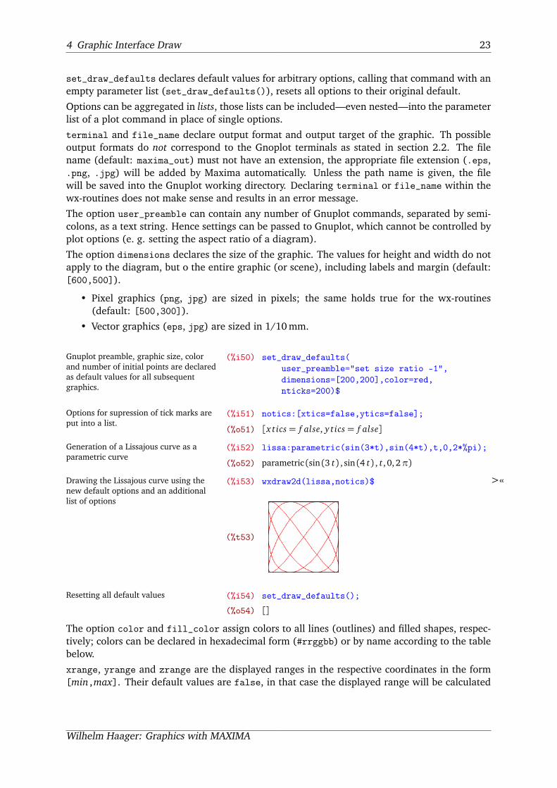
Gnuplot preamble, graphic size, colorand number of initial points are declaredas default values for all subsequentgraphics.

(%i50) set_draw_defaults(user_preamble="set size ratio -1",dimensions=[200,200],color=red,nticks=200)$

Options for supression of tick marks areput into a list.

(%i51) notics:[xtics=false,ytics=false];

(%o51) [x tics = f alse, y tics = f alse]

Generation of a Lissajous curve as aparametric curve

(%i52) lissa:parametric(sin(3*t),sin(4*t),t,0,2*%pi);

(%o52) parametric (sin (3 t) , sin (4 t) , t, 0, 2π)

Drawing the Lissajous curve using thenew default options and an additionallist of options

(%i53) wxdraw2d(lissa,notics)$

(%t53)

>«

Resetting all default values (%i54) set_draw_defaults();

(%o54) []

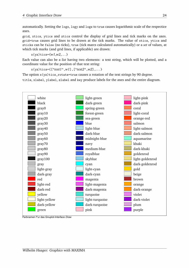
The option color and fill_color assign colors to all lines (outlines) and filled shapes, respec-tively; colors can be declared in hexadecimal form (#rrggbb) or by name according to the tablebelow.

xrange, yrange and zrange are the displayed ranges in the respective coordinates in the form[min,max]. Their default values are false, in that case the displayed range will be calculated



automatically. Setting the logx, logy and logz to true causes logarithmic scale of the respecticeaxes.

grid, xtics, ytics and ztics control the display of grid lines and tick marks on the axes.grid=true causes grid lines to be drawn at the tick marks. The value of xtics, ytics andzticks can be false (no ticks), true (tick marcs calculated automatically) or a set of values, atwhich tick marks (and grid lines, if applicable) are drawn:

x(yz)tics={w1,w2,. . . }

Each value can also be a list having two elements: a text string, which will be plotted, and acoordinate value for the position of that text string:

x(yz)tics={["text1",w1],["text2",w2],. . . }

The option x(yz)tics_rotate=true causes a rotation of the text strings by 90 degree.

title, xlabel, ylabel, zlabel and key produce labels for the axes and the entire diagram.

white light-green light-pinkblack dark-green dark-pinkgray0 spring-green coralgray10 forest-green light-coralgray20 sea-green orange-redgray30 blue salmongray40 light-blue light-salmongray50 dark-blue dark-salmongray60 midnight-blue aquamarinegray70 navy khakigray80 medium-blue dark-khakigray90 royalblue goldenrodgray100 skyblue light-goldenrodgray cyan dark-goldenrodlight-gray light-cyan golddark-gray dark-cyan beigered magenta brownlight-red light-magenta orangedark-red dark-magenta dark-orangeyellow turquoise violetlight-yellow light-turquoise dark-violetdark-yellow dark-turquoise plumgreen pink purple

Farbnamen f"ur das Gnuplot-Interface Draw



Set of values for scale ticks along they-axis and horizontal grid lines

(%i55) yt:setify(create_list(signum(n)*sqrt(abs(n)),n,[-4,-3,-1,0,1,3,4])/2);

(%o55) −1,−1

2, 0,

1

2,1,−p

3

2,

p3

2

Values for scale ticks along the x-axisand vertical grid lines as lists, eachcontaining a text string and thex-coordinate

(%i56) xt:setify(makelist([string(30*n),30*n*%pi/180],n,0,12));

(%o56) {[0, 0], [120,2π

3], [150,

5π

6], [180,π], [210,

7π

6],

[240,4π

3], [270,

3π

2], [30,

π

6], [300,

5π

3], [330,

11π

6],

[360, 2π], [60,π

3], [90,

π

2]}

Sine curve with gridlines and tick marks (%i57) wxdraw2d(yrange=[-1.5,1.5],xtics=xt,ytics=yt,grid=true,color=red,explicit(sin(x),x,0,2*%pi),xlabel="phi (Grad)",ylabel="sin(phi)")$

(%t57)

Point plots (graphic object points) accept the option point_type with an integer value between−1 and 16 or a name according to the table below:

-1 $none 4 square 9 filled_up_triangle0 dot 5 filled_square 10 down_triangle1 plus 6 circle 11 filled_down_triangle2 multiply 7 filled_circle 12 diamant3 asterisk 8 up_triangle 13 filled_diamant

Possible values of the option point_type

Declaring points along a sine curve as agraphic object

(%i58) sine:points(float(map(lambda([u],[u,sin(u)]),makelist(u,u,-6,6)/2)));

(%o58) points([[−3.0,−0.141], [−2.5,−0.598], [−2.0,−0.909],[−1.5,−0.997], [−1.0,−0.841], [−0.5,−0.479], [0.0, 0.0],[0.5, 0.479], [1.0,0.841], [1.5, 0.997], [2.0, 0.909], [2.5,0.598],[3.0, 0.141]])



Declaring points along a straight line asa graphic object

(%i59) line:points(float(makelist([k,-k/4],k,-3,3)));

(%o59) points([[−3.0, 0.75], [−2.0, 0.5], [−1.0,0.25], [0.0, 0.0],[1.0,−0.25], [2.0,−0.5], [3.0,−0.75]])

Sine function and two point plots: Pointsalong the sine function, as well as pointsalong a straight line, connected by linesegments.

(%i60) wxdraw2d(color=blue,line_width=2,explicit(sin(x),x,-%pi,%pi),color=red,point_size=2,point_type=7,sine,points_joined=true,point_type=4,color=green,line)$

(%t60)

4.5 Options for Labels and Vectors

label_alignment=value Alignment of the label; possible values: center(default), left, right

label_orientation=value Orientation of the label; possible values: horizontal(default), vertical

head_length=len Length of the arrowheads of vectors in units of thex-axis (default: 2)

head_angle=winkel Angle between arrow heads and segment in degrees(default: 45)

head_type=typ Type of the arrow head of vectors; possible values:filled (default), empty, nofilled

head_both=true/false Decides, whether vectors are plotted with two arrowheads

Options for labels and vectors

Three text strings (%i61) [l1,l2,l3]:["left aligned label","centered label","rigt aligned label"]$

Assigning long option names to shortvariable names unburdens subsequentwriting.

(%i62) [la,hs,ha,hl]:[label_alignment,head_size,head_angle,head_length]$



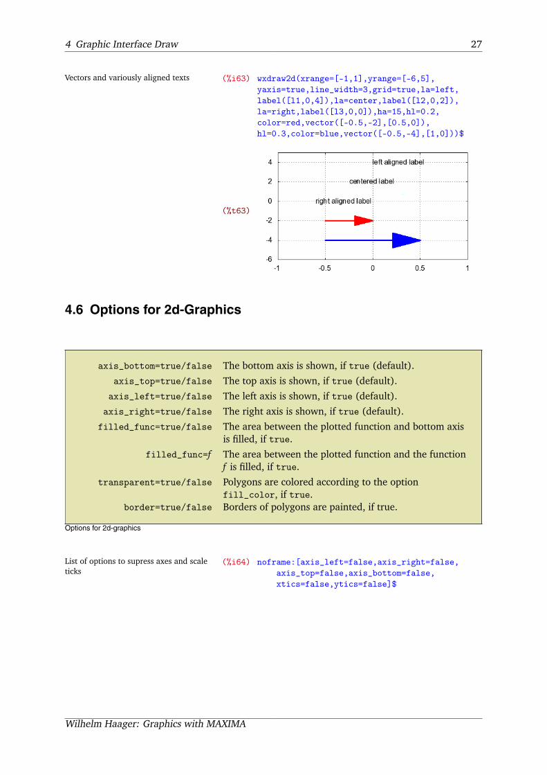
Vectors and variously aligned texts (%i63) wxdraw2d(xrange=[-1,1],yrange=[-6,5],yaxis=true,line_width=3,grid=true,la=left,label([l1,0,4]),la=center,label([l2,0,2]),la=right,label([l3,0,0]),ha=15,hl=0.2,color=red,vector([-0.5,-2],[0.5,0]),hl=0.3,color=blue,vector([-0.5,-4],[1,0]))$

(%t63)

4.6 Options for 2d-Graphics

axis_bottom=true/false The bottom axis is shown, if true (default).

axis_top=true/false The top axis is shown, if true (default).

axis_left=true/false The left axis is shown, if true (default).

axis_right=true/false The right axis is shown, if true (default).

filled_func=true/false The area between the plotted function and bottom axisis filled, if true.

filled_func=f The area between the plotted function and the functionf is filled, if true.

transparent=true/false Polygons are colored according to the optionfill_color, if true.

border=true/false Borders of polygons are painted, if true.

Options for 2d-graphics

List of options to supress axes and scaleticks

(%i64) noframe:[axis_left=false,axis_right=false,axis_top=false,axis_bottom=false,xtics=false,ytics=false]$



Drawing various shapes with variousoptions

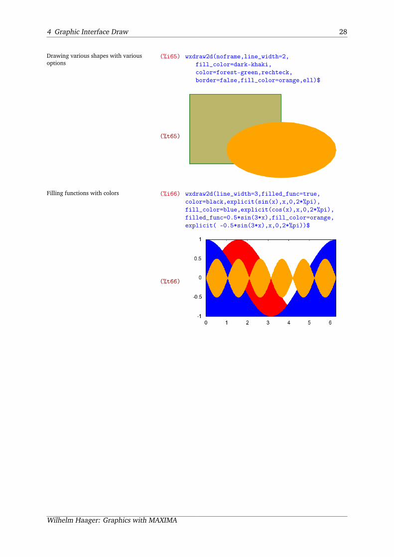
(%i65) wxdraw2d(noframe,line_width=2,fill_color=dark-khaki,color=forest-green,rechteck,border=false,fill_color=orange,ell)$

(%t65)

Filling functions with colors (%i66) wxdraw2d(line_width=3,filled_func=true,color=black,explicit(sin(x),x,0,2*%pi),fill_color=blue,explicit(cos(x),x,0,2*%pi),filled_func=0.5*sin(3*x),fill_color=orange,explicit( -0.5*sin(3*x),x,0,2*%pi))$

(%t66)



4.7 Options for 3d-Graphics

view=[ϕ,ϑ] Setting the view angle: ϕ. . . around the x-axis,ϑ. . . around the z-axis

axis_3d=true/false Display of all axes in 3d-graphics (default: true)

xu_grid=n Number of coordinates along the x-axis for drawinggrid lines

yv_grid=n Number of coordinates along the y-axis for drawinggrid lines

surface_hide=true/false Controls the visibility of hidden parts of 3d-surfaces

enhanced3d=true/false Controls coloring of 3d-surfaces

palette=[r,g,b] Numbers of the color palettes of the red, green andblue components for image objects and 3d-surfaces

colorbox=true/false Draws a color scale into the diagram, which uses acolor palette, if true (default)

contour=value Controls contour lines of 3d-surfaces; possible values:none (default), base, surface, both, map

contour_levels=n n contour lines are drawn at equal intervals.

contour_levels=[x1,dx,x2] Contour lines are plotted at values from x1 to x2 withan interval of dx

contour_levels={x1,x2,. . . } Contour lines are plotted at the specified levels x1, x2,etc.

ip_grid=[nx,ny] Number of initial grid points in implicit plots(default: [50,50])

ip_grid_in=[nx,ny] Number of secondary grid points in implicit plots(default: [5,5])

Options for 3d-graphics

The option view=[ϕ,ϑ] defines the view on the 3d-graphic with a list containing two ele-ments:

• ϕ is the rotation around the x-axis in degree; ϕ=0 means horizontal view, ϕ=90 meansview from above.

• ϑ is the rotation around the z-axis in degree; ϑ=0 means front view, ϑ=90 means viewfrom the side.

axis_3d controls the display of all axes in 3d-graphics. To supress the display of the axes entirely,additional to the option axis_3d=false also the tick marks must be turned off using the optionx(xz)tics=false.

xu_grid and yv_grid define the number of coordinates for grid lines along the x-axis and they-axis. The number of grid lines in the respective direction is by 1 higher than the value of thatoption. The grid points are connected by line segments. Thus the surface is displayed the moreaccurately, the higher those values are.



Declaration of a function in twovariables

(%i67) f:2/(x^2+y^2+1)+1/((x-5)^2+y^2+1);

(%o67)2

y2 + x2 + 1+

1

y2 + (x − 5)2 + 1

Generation of a graphic object (%i68) g:explicit(f,x,-2,10,y,-6,6)$

3D-display of the function (%i69) wxdraw3d(xtics=false,ytics=false,ztics=false,axis_3d=false,xu_grid=50,color=red,surface_hide=true,g)$

(%t69)

If the option enhanced3d is set to true, the surfaces are colored with a color gradient, whichalways depends on the z-axis. The color gradient can be defined with the option palette.Herein the color function can be selected with a number between 0 and 26, separately for red,green and blue value. The color functions are stated in [1].

Th option colorbox controls the display of a color scale showing the color gradient.

Function with colored surface. Theentire color palette, displayed in a colorscale, always fills the entire range of thez coordinate, independently of minimumand maximum values of the function.

(%i70) wxdraw3d(xtics=false,ytics=false,ztics=false,axis_3d=false,xu_grid=50,enhanced3d=true,surface_hide=true,view=[90,0],g)$

(%t70)

The option contours controls the display of contour lines, the following values are possible:

• none: No contour lines are drawn (default).

• base: Contour lines are projected into the xy-plane.

• surface: Contour lines are drawn on the surface.

• both: Contour lines are drawn both in the xy-plane and on the surface.

• map: View from above (corresponds to rot_vertical=0), grid lines are not displayed.



The option contour_levels declares the number and the values of contour lines.

Display of contour lines on the surface (%i71) wxdraw3d(xtics=false,ytics=false,ztics=false,axis_3d=false,contour_levels=10,contour=surface,g)$

(%t71)

Displaying the function as contour plot (%i72) wxdraw3d(xtics=false,ytics=false,ztics=false,axis_3d=false,contour_levels=10,contour=map,g)$

(%t72)


Bibliography 32

Bibliography

[1] Maxima Development Team: Maxima Reference Manual V.5.23. 2011.

[2] Philipp K. Janert: Gnuplot in Action, Understanding Data with Graphs. ManningPublications 2009.

[3] Mario Rodríguez Riotorto: A Maxima-Gnuplot Interface.http://www.telefonica.net/web2/biomates/maxima/gpdraw.


graphics with maxima - austromath · graphics with maxima (version 5.23 and above) wilhelm haager...

Documents