graphs basics 10152010
TRANSCRIPT

8/10/2019 Graphs Basics 10152010
http://slidepdf.com/reader/full/graphs-basics-10152010 1/23
Examples of two- and three-dimensional graphics in Smath Studio
---------------------------------------------------------------
By Gilberto E. Urroz, October 2010
Basic__commands__using__the__"Insert"__menu:
To insert a two-dimensional (2D) graph, use: Insert > Plot > 2D
To insert a three-dimensional(3D) graph, use: Insert > Plot > 3D
EXAMPLE 1A - Plotting a single function of x:
sin x
-16 -8 0 8 16
12
8
4
0
-4
-8
x
y
1 - Click on point in your worksheetwhere you want to set the upperleft corner of graph
2 - Click on the "2D" icon in the"Functions" palette or use the"Insert > Graph > 2D" menu option
3 - Type the function name in theplaceholder below the graph.
In this example we plot thefunction: f(x) = sin(x)
Thus, type: "sin(x)", then clicksomewhere in the worksheet outsideof the graph.
EXAMPLE 1B - Plotting a single function of (x,y):
sin yx
xy
z
0 22
2
4
4
4
66
6
1 - Click on point in your worksheetwhere you want to set the upperleft corner of graph
2 - Click on the "3D" icon in the"Functions" palette or use the"Insert > Graph > 3D" menu option
3 - Type the function name in theplaceholder below the graph.
In this example we plot thefunction: f(x) = x*sin(y)
Thus, type: "x*sin(y)", then clicksomewhere in the worksheet outsideof the graph.
Using__icons__in__the__"Functions"__palette:
Click on the "2D" or "3D" icon in the palette
to insert a 2D or 3D graph: -> -> -> -> -> -> -> ->
Also, use the "Multiple Values" icon -> ->to plot more than one function.
EXAMPLE 2A - Plotting two functions of x in 2D:
20Oct201007:26:36-GraphsBasics10152010_ForPrinting.sm
1/23
8/10/2019 Graphs Basics 10152010
http://slidepdf.com/reader/full/graphs-basics-10152010 2/23
cos x
sin x
-16 -8 0 8 16
12
8
4
0
-4
-8
x
y
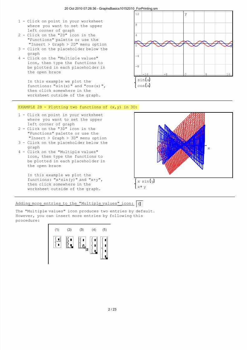
1 - Click on point in your worksheetwhere you want to set the upperleft corner of graph
2 - Click on the "2D" icon in the"Functions" palette or use the"Insert > Graph > 2D" menu option
3 - Click on the placeholder below thegraph
4 - Click on the "Multiple values"icon, then type the functions tobe plotted in each placeholder inthe open brace
In this example we plot thefunctions: "sin(x)" and "cos(x)",then click somewhere in theworksheet outside of the graph.
EXAMPLE 2B - Plotting two functions of (x,y) in 3D:
1 - Click on point in your worksheetwhere you want to set the upperleft corner of graph
2 - Click on the "3D" icon in the"Functions" palette or use the"Insert > Graph > 3D" menu option
3 - Click on the placeholder below thegraph
4 - Click on the "Multiple values"icon, then type the functions tobe plotted in each placeholder inthe open brace
In this example we plot thefunctions: "x*sin(y)" and "x+y",
then click somewhere in theworksheet outside of the graph.
yx
sin yx
xy
z
0 22
2
44
4
66
6
Adding__more__entries__to__the__"Multiple__values"__icon:
The "Multiple values" icon produces two entries by default.However, you can insert more entries by following thisprocedure:
20Oct201007:26:36-GraphsBasics10152010_ForPrinting.sm
2/23
8/10/2019 Graphs Basics 10152010
http://slidepdf.com/reader/full/graphs-basics-10152010 3/23
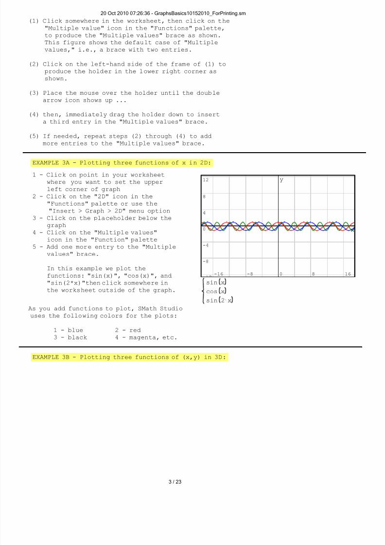
(1) Click somewhere in the worksheet, then click on the"Multiple value" icon in the "Functions" palette,to produce the "Multiple values" brace as shown.This figure shows the default case of "Multiplevalues," i.e., a brace with two entries.
(2) Click on the left-hand side of the frame of (1) toproduce the holder in the lower right corner asshown.
(3) Place the mouse over the holder until the doublearrow icon shows up ...
(4) then, immediately drag the holder down to inserta third entry in the "Multiple values" brace.
(5) If needed, repeat steps (2) through (4) to addmore entries to the "Multiple values" brace.
EXAMPLE 3A - Plotting three functions of x in 2D:
1 - Click on point in your worksheetwhere you want to set the upper
left corner of graph2 - Click on the "2D" icon in the"Functions" palette or use the"Insert > Graph > 2D" menu option
3 - Click on the placeholder below thegraph
4 - Click on the "Multiple values"icon in the "Function" palette
5 - Add one more entry to the "Multiplevalues" brace.
In this example we plot thefunctions: "sin(x)", "cos(x)", and"sin(2*x)"then click somewhere inthe worksheet outside of the graph.
sin x2
cos x
sin x
-16 -8 0 8 16
12
8
4
0
-4
-8
x
y
As you add functions to plot, SMath Studiouses the following colors for the plots:
1 - blue 2 - red3 - black 4 - magenta, etc.
EXAMPLE 3B - Plotting three functions of (x,y) in 3D:
20Oct201007:26:36-GraphsBasics10152010_ForPrinting.sm
3/23

8/10/2019 Graphs Basics 10152010
http://slidepdf.com/reader/full/graphs-basics-10152010 4/23
1 - Click on point in your worksheetwhere you want to set the upperleft corner of graph
2 - Click on the "3D" icon in the"Functions" palette or use the"Insert > Graph > 3D" menu option
3 - Click on the placeholder below thegraph
4 - Click on the "Multiple values"icon in the "Function" palette
5 - Add one more entry to the "Multiplevalues" brace.
In this example we plot thefunctions: "x*sin(y)", "x+y", and"x-y"then click somewhere inthe worksheet outside of the graph.
yx
yx
sin yx
xy
z
0 22
2
44
4
66
6
Icons__in__the__"Plot"__palette: -> -> -> -> -> -> ->
(1) Rotate: Rotate a 3D graph only(2) Scale:(see instructions below)
(3) Move: drag graph up or down, left or right(4) Graph by points: show points instead of lines(5) Graph by lines: show lines (default)(6) Refresh: restore to original version of graph
Detalles__of__"Scale"__in__a__2D__graph:
* ZOOM IN or OUT: Click on the "Scale" icon, icon (2), then click onthe graph (also for 3D plots):- ZOOM IN: Drag the mouse inwards, towards the origin, to decreasesize of axes divisions
- ZOOM OUT: Drag the mouse outwards, away from the origin, to increasesize of axis divisions
* Alternatively, to ZOOM IN or OUT, click on the "Scale" icon, clickinside the graph and use the mouse wheel (also for 3D plots):- ZOOM IN: roll mouse wheel up- ZOOM OUT: roll mouse wheel down
* ZOOM IN or OUT on the x-axis only: Click on the "Scale" icon, clickon the graph, hold the [SHIFT] key, then:- ZOOM IN X-AXIS: roll mouse wheel up- ZOOM OUT X-AXIS: roll mouse wheel down
* ZOOM IN or OUT on the y-axis only: Click on the "Scale" icon, clickon the graph, hold the [CTRL] key, then:- ZOOM IN Y-AXIS: roll mouse wheel up
- ZOOM OUT Y-AXIS: roll mouse wheel down
EXAMPLE 4A - Changing the size of the graph window in 2D:
Click on the graph window, then drag one of the three black handlers inthe graph window to adjust its size
1
20Oct201007:26:36-GraphsBasics10152010_ForPrinting.sm
4/23
8/10/2019 Graphs Basics 10152010
http://slidepdf.com/reader/full/graphs-basics-10152010 5/23
sin x
0
64
48
32
16
0
-16
-32
-48
-64
x
y (2)
sin x
-8 -4 0 4 8
2
0
-2
x
y
(3)
sin x
-16 -8 0 8
8
4
0
-4
-8
x
y
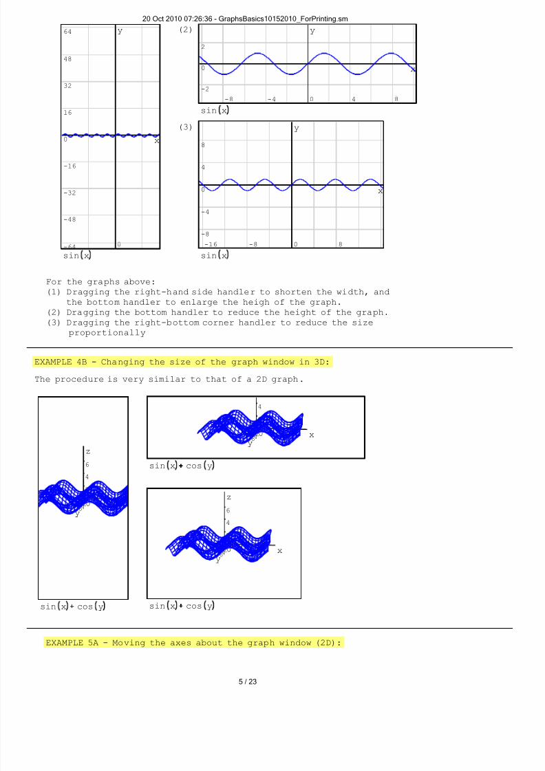
For the graphs above:(1) Dragging the right-hand side handler to shorten the width, and
the bottom handler to enlarge the heigh of the graph.(2) Dragging the bottom handler to reduce the height of the graph.(3) Dragging the right-bottom corner handler to reduce the size
proportionally
EXAMPLE 4B - Changing the size of the graph window in 3D:
The procedure is very similar to that of a 2D graph.
cos ysin x
y
z
0 22
2
44
4
66
6 cos ysin x
xy
0 22
2
44
4
66
cos ysin x
xy
z
0 22
2
44
4
66
6
EXAMPLE 5A - Moving the axes about the graph window (2D):
20Oct201007:26:36-GraphsBasics10152010_ForPrinting.sm
5/23
8/10/2019 Graphs Basics 10152010
http://slidepdf.com/reader/full/graphs-basics-10152010 6/23
sin x
-16 -8 0 8 16
12
8
4
0
-4
-8
x
y
sin x
-8 0 8 16 24
4
0
-4
-8
-12
-16
x
y
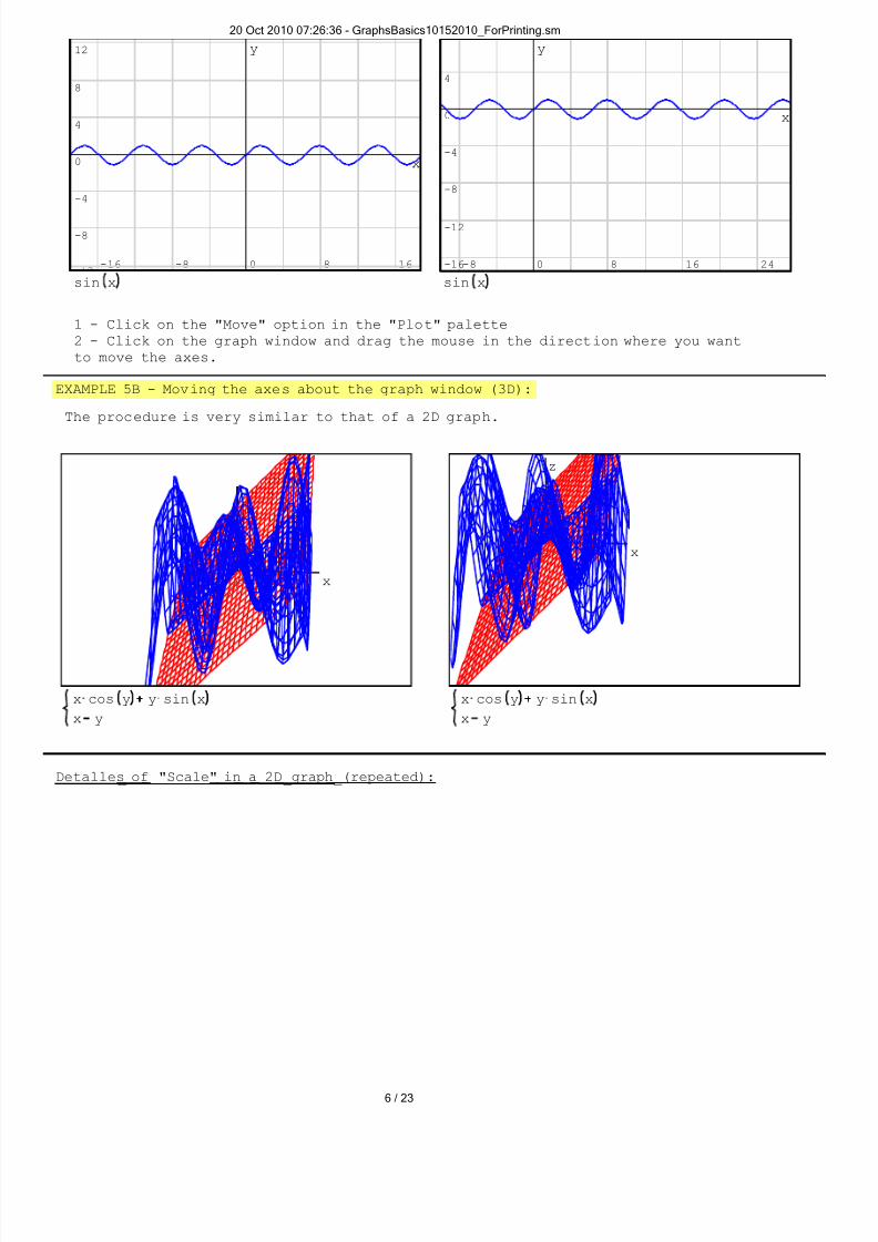
1 - Click on the "Move" option in the "Plot" palette2 - Click on the graph window and drag the mouse in the direction where you wantto move the axes.
EXAMPLE 5B - Moving the axes about the graph window (3D):
The procedure is very similar to that of a 2D graph.
yx
sin xycos yx
xy
z
0 22
2
44
4
66
6
yx
sin xycos yx
xy
z
0 22
2
44
4
66
6
Detalles__of__"Scale"__in__a__2D__graph__(repeated):
20Oct201007:26:36-GraphsBasics10152010_ForPrinting.sm
6/23

8/10/2019 Graphs Basics 10152010
http://slidepdf.com/reader/full/graphs-basics-10152010 7/23
* ZOOM IN or OUT: Click on the "Scale" icon, icon (2), then click onthe graph (also for 3D plots):- ZOOM IN: Drag the mouse inwards, towards the origin, to decreasesize of axes divisions
- ZOOM OUT: Drag the mouse outwards, away from the origin, to increasesize of axis divisions
* Alternatively, to ZOOM IN or OUT, click on the "Scale" icon, clickinside the graph and use the mouse wheel (also for 3D plots):- ZOOM IN: roll mouse wheel up
- ZOOM OUT: roll mouse wheel down
* ZOOM IN or OUT on the x-axis only: Click on the "Scale" icon, clickon the graph, hold the [SHIFT] key, then:- ZOOM IN X-AXIS: roll mouse wheel up- ZOOM OUT X-AXIS: roll mouse wheel down
* ZOOM IN or OUT on the y-axis only: Click on the "Scale" icon, clickon the graph, hold the [CTRL] key, then:- ZOOM IN Y-AXIS: roll mouse wheel up- ZOOM OUT Y-AXIS: roll mouse wheel down
EXAMPLE 6A - Scaling (zooming) a 2D graph:
sin x
-2 -1 0 1 2
12
8
4
0
-4
-8
x
y <--- To zoom the x-axis only:1 - Click on "Scale" in the "Plot" palett2 - Click on the graph window3 - Hold down the "Shift" key4 - Roll the mouse wheel up or down
sin x
-16 -8 0 8 16
1
0.5
0
-0.5
-1
x
y
To zoom the y-axis only: ---->1 - Click on "Scale" in the "Plot" palette2 - Click on the graph window3 - Hold down the "Control" key4 - Roll the mouse wheel up or down
20Oct201007:26:36-GraphsBasics10152010_ForPrinting.sm
7/23

8/10/2019 Graphs Basics 10152010
http://slidepdf.com/reader/full/graphs-basics-10152010 8/23
sin x
-6 -4 -2 0 2 4 6
0.75
0.5
0.25
0
-0.25
-0.5
-0.75
x
y
<--- You can zoom both axes by zooming oneaxis at a time. In this case, I zoomedthe x axis first, and then the y axis.
Note: Use the "Refresh" option in the "Plot" menuto recover the original version of any plot.
EXAMPLE 6B - Scaling (zooming) a 3D graph:
cos yx
sin yx
xy
z
0 22
2
44
4
66
6
cos yx
sin yx
xy
z
0 11
1
22
2
Examples__of__other__types__of__graphs__in__2-D
The following examples show other ways to produce 2D graphics. Data fora graph y = f(x) can be generated by using a vector of values of x, thengenerating a vector of values of y. The two vectors are then puttogether into a matrix, whose name is used in the 2D graph placeholderinstead of f(x).
EXAMPLE 7 - Plotting a function using vectors:
Vectors of x and y data are created using ranges,example:
, ..20
ππ ππx
Create x vector as followsType: x : range - p cntl-G , p cntl-G ,
- p cntl-G + p cntl-G / 20
length xnCalculate the length of vector = n
41n
20Oct201007:26:36-GraphsBasics10152010_ForPrinting.sm
8/23

8/10/2019 Graphs Basics 10152010
http://slidepdf.com/reader/full/graphs-basics-10152010 9/23
Fill out y vector using a for loop. Click "for"in the "Programming" palette, then use:range 1 , n
Use sub-indices, e.g., y [ k ... etc.
for
sink
x22
sink
xk
y
..n1k
augment , yxM Form augmented matrix M with vectors x and y,place M in graph as a function name:
M
-2 0 2
1.5
1
0.5
0
-0.5
x
y
< --- The graph was zoomed in and the axesmoved by using the following procedures:
1 - To zoom x-axis only: click on "Scale" inthe "Plot" palette, hold the "Control" keyand use the mouse wheel
2 - To zoom y-axis only: click on "Scale" inthe "Plot" paletted, hold the "Shift" keyand use the mouse wheel
3 - To move axes, drag mouse across graph wind
Using points or lines for a plot:
M
-4 -2 0 2
2
1.5
1
0.5
0
-0.5
-
x
yUsing the sparse data in matrix M we reprothe graph above, but then we selected the"Graph by points" option in the "Plot" palto produce the graph shown to the left.
You can click the option "Graph by lines"option in the "Plot" palette to return tothe default graph format of continuous lin
EXAMPLE 8 - Plotting a function and a matrix
In this example we plot the function y = cos(x) anda matrix M with vector data of y = sin(x) in the range-π < x < π.
, ..20
ππ ππx length xn 41n
for
sink
xk
y
..n1k
augment , yxM
20Oct201007:26:36-GraphsBasics10152010_ForPrinting.sm
9/23

8/10/2019 Graphs Basics 10152010
http://slidepdf.com/reader/full/graphs-basics-10152010 10/23
cos x
M
-16 -8 0 8 16
12
8
4
0
-4
-8
x
y
cos x
M
-8 -6 -4 -2 0 2 4 6 8
1
0.5
0
-0.5
-1
x
y
1 - Original graph 2 - Zooming In in both x and y
EXAMPLE 9 - Parametric plots in 2D using matrices:
Parametric plots are plots of the form x = x(t), y = y(t).A parametric plot can be generated by using vectors andmatrices as illustrated below. Use a fine grid for theparameter t to produce a continuous curve.
, ..50
ππ ππt Define the vector of the parameter t
length tn Determine length of vector t = n
for
cos
k
t22
k
y
sink
t3k
x
..n1kCalculate vectors of x = x(t) andy = y(t)
Produce matrix of (x,y) and plot itaugment , yxM
M
-1 -0.5 0 0.5 1
2
1
0
-1
-2
x
y
M
-1 -0.5 0 0.5 1
2
1
0
-1
-2
x
y
1 - Using "Plot by Lines" optionin the "Plot" palette
2 - Using "Plot by Lines" optionin the "Plot" palette
EXAMPLE 10 - Polar plots produced using vectors and matrices:
20Oct201007:26:36-GraphsBasics10152010_ForPrinting.sm
10/23

8/10/2019 Graphs Basics 10152010
http://slidepdf.com/reader/full/graphs-basics-10152010 11/23
Polar plots are similar to parametric plots. In polar plots theindependent variable is the angle θ, and the dependent variableis the radial position r, i.e., r = f(θ). To produce the plotthe (x,y) coordinates are calculated using x = r*cos(θ) andy = r*sin(θ) as illustrated below.
, ..50
ππ20θ Generate vector of θ between 0 and 2π
length θn Determine lenght of vector θ
for
sink
θ212k
r
..n1k Generate values of r = f(θ)
for
sink
θk
rk
yy
cosk
θk
rk
xx
..n1kGenerate coordinates:
x = r cos(θ)y = r sin(θ)
augment , yyxxP Produce matrix of (x,y) and plot it
P
-4 -2 0 2 4
6
5
4
3
2
1
0
-
x
y
P
-4 -2 0 2 4
6
5
4
3
2
1
0
-
x
y
1 - Using "Plot by Lines" optionin the "Plot" palette
2 - Using "Plot by Lines" optionin the "Plot" palette
EXAMPLE 11 - Parametric plot in three-dimensions- space curves
Parametric equations of the form x = x(t), y = y(t), z = z(t),produces a space curve. To generate the graph, use a vector ofvalues of t, and then calculate the corresponding vectors ofvalues of x, y, and z. Put together a matrix whose columns arethe x,y,z data, and use a 3D plot.
, ..0.1 100t Create a vector t with values of the parameter thatwill produce x = x(t), y = y(t), and z = z(t).
length tn Determine the length of vector t
101n
20Oct201007:26:36-GraphsBasics10152010_ForPrinting.sm
11/23

8/10/2019 Graphs Basics 10152010
http://slidepdf.com/reader/full/graphs-basics-10152010 12/23
for
2
kt
kz
cosk
tk
y
sink
tk
x
..n1k Generate vectors x, y, and z using a "for" loop
augment , , zyxMBuild matrix M with coordinates (x,y,z)
M
xy
z
0 22
2
44
4
66
6
Plot matrix M in a 3D plot
EXAMPLE 12 - Using 2D graphs in solving equations:
In this example we seek the solution(s) for the equation:
5x23
x12
x
A solution can be found by determining the intersection of the functions:
12
xf x 5x23
xg x
Using graphics and zooming the intersection we estimate the solution to be close tox = 1.80
g x
f x
-4 -2 0 2 4
16
12
8
4
0
-
x
y
g x
f x
1.625 1.6875 1.75 1.8125 1.875
4.375
4.25
4.125
4
3.875
1.78solve , x5x23
x12
xThe exact solution can be found using:
20Oct201007:26:36-GraphsBasics10152010_ForPrinting.sm
12/23

8/10/2019 Graphs Basics 10152010
http://slidepdf.com/reader/full/graphs-basics-10152010 13/23
EXAMPLE 12 - Graphical solution for a pump-pipeline system (Civil EngineeringHydraulics)
Solution:=========
Write out all the given data without units, but using theproper set of units for the English System:
6105ee1000L (ft) 0.15D (ft) (ft) 6Δz (ft)
5101.2ν (ft^2/s) 32.2g (m/s^2) 6.01.00.5ΣKm , i.e., 7.5ΣKm
For the pump: 14.09a 138.02b 2267.62c
Using the Swamee-Jain equationfor the friction factor: 2
log100.9
r
5.74
3.7
k
0.25fSJ , rk
D
LfSJ ,
Dνπ
Q4
D
eeΣKm
4Dg
2π
2Q8
ΔzhPthe system equation becomes: [1]
2QcQbahP
[2]The pump equation is:
A graphical analysis shows the solution as the intersection of thesystem and the pump curves, i.e.,
D
LfSJ ,
Dνπ
Q4
D
eeΣKm
4Dg
2π
2Q8
ΔzhP1 Q 2
QcQbahP2 Q
20Oct201007:26:36-GraphsBasics10152010_ForPrinting.sm
13/23

8/10/2019 Graphs Basics 10152010
http://slidepdf.com/reader/full/graphs-basics-10152010 14/23
hP2 x
hP1 x
0 0.015625 0.03125 0.0468750.0625 0.07
16
14
12
10
8
6
4
2
0
-2
x
y
Notice that, even though we defined hP1 andhP2 as functions of Q, when using the 2D plot,we need to define them as functions of x.
The exact solution can be found by solving the equation: hP1(Q)=hP2(Q)
2103.01solve , , , 10QhP2 QhP1 Q
EXAMPLE 14 - More examples of three-dimensionalgraphs - surfaces:
yx
xy
z
0 22
2
4
4
4
66
6
yx
x
y
z
0 2
2
2
4
4
4
6
6
6
8
8
8
Use the option "3D" in the "Functions" palette,and enter the function f(x,y) in the place-holder. The result is a 3D surface, in thiscase, a plane. The original plot is shownabove.
Use the "Rotate" option in the "Plot" pato change the surface view.
20Oct201007:26:36-GraphsBasics10152010_ForPrinting.sm
14/23

8/10/2019 Graphs Basics 10152010
http://slidepdf.com/reader/full/graphs-basics-10152010 15/23

8/10/2019 Graphs Basics 10152010
http://slidepdf.com/reader/full/graphs-basics-10152010 16/23

8/10/2019 Graphs Basics 10152010
http://slidepdf.com/reader/full/graphs-basics-10152010 17/23
2y
2x
2y
2x5
xy
z
0 33
3
66
6
99
9
sin y
sin x
x
y
z
0 22
2
4
4
4
6
6
6
8
8
8
EXAMPLE 17 - Drawing a surface and a space curve together:
Myx
x
y
z
0 2
2
24
4
4
6
6
6
8
8
8
Use the "Multiple values"option in the "Plot" palette,and enter the equation of thesurface (e.g., x+y) and thematrix that represents thespace curve (e.g., M)
EXAMPLE 18 - Plotting 2 space curves:
In this example two straight lines in 3D areproduced by using linear parametric equations., ..1.9 22t
Vector t is the parameter, and the coordinatesof the two curves are given by (x1,y1,z1) and(x2,y2,z2). These lines are represented by thematrices P and Q, respectively.
length tn
40n
for
kt81
kz1
kt41
ky1
kt51
kx1
..n1k for
kt
kz2
kt1
ky2
kt31
kx2
..n1k
augment , , z1y1x1P augment , , z2y2x2Q
20Oct201007:26:36-GraphsBasics10152010_ForPrinting.sm
17/23

8/10/2019 Graphs Basics 10152010
http://slidepdf.com/reader/full/graphs-basics-10152010 18/23
P
xy
z
0 22
2
44
4
66
6
Q
xy
z
0 22
2
44
4
66
6
Individual plots of curves given by matrices P and Q.
Q
P
xy
z
0 22
2
44
4
66
6
<--- Join plot oflines givenby matricesP and Q
Plot__specifications __using__SMath__Studio__0.89__-__Release__8
SMath Studio 0.89 - Release 8 includes the ability of specifiyingfour different types of symbols for the graphs, modifying thesize of the symbols, and select the color of the symbol. This isaccomplished by building a matrix that includes the coordinates(x,y), the character, its size, and the color, in that order.
* Characters: you can select for plotting the characters:"x" "*" "." "o"
* Size: given in pixels, e.g., 5, 10, 20, 100, etc.
* Colors available (figure below split for printing purposes):
20Oct201007:26:36-GraphsBasics10152010_ForPrinting.sm
18/23

8/10/2019 Graphs Basics 10152010
http://slidepdf.com/reader/full/graphs-basics-10152010 19/23
You can write them in lower case lettes , as shown above, or all in uppercase letters, or combinations of upper and lower case letters. For example,
you could write in your color specification "darkblue", "DARKBLUE", or"DarkBlue", and the result would be the same. Additionally, you can havespaces in the color specification which will be ignored by SMath Studio inproducing the output to the graphic canvas. For example, you can write"Dark Blue", and it will be interpreted as "darkblue".
NOTE: Any color combination, such as "LightRed", not defined above,will produce, by default, the color black.
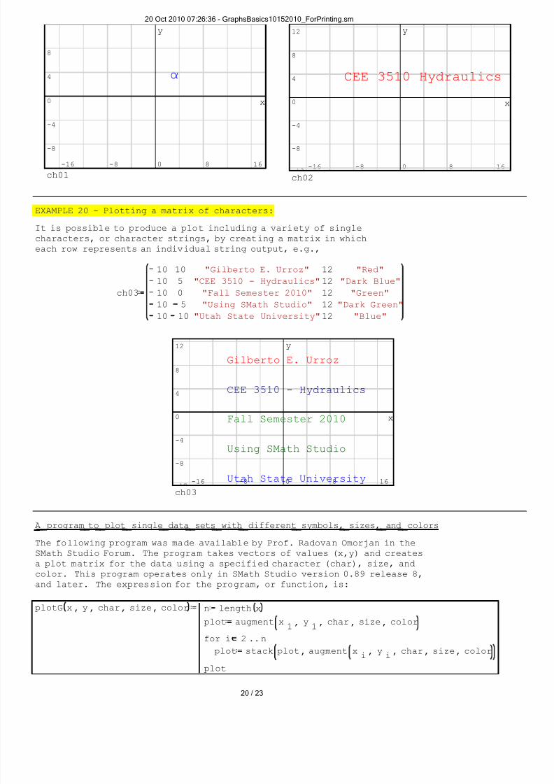
EXAMPLE 19 - Plotting a single character or a character string:
You can define a row vector with the properties: (x,y,char,size,color)to write a single character or a string of characters, e.g.,
"Blue"15"α"52ch01 "red15"CEE 3510 Hydraulics"510ch02
20Oct201007:26:36-GraphsBasics10152010_ForPrinting.sm
19/23
8/10/2019 Graphs Basics 10152010
http://slidepdf.com/reader/full/graphs-basics-10152010 20/23

8/10/2019 Graphs Basics 10152010
http://slidepdf.com/reader/full/graphs-basics-10152010 21/23
EXAMPLE 21 - Plotting data (x,y) with function "plotG"
The following graphs show the plotting of the function y = sin(x),with values of x between 0 and 10, in increments of 0.5, usingdifferent symbols, sizes, and colors. The data is generated here:
, ..0.5 100x length xn 21n
for
sin kxky
..n1k
The plots are shown below:
plotG , , , , "Light Green"25"."yxplot1 plotG , , , , "Magenta"35"+"yxplot2
plot1
0 2 4 6 8 10
1.5
1
0.5
0
-0.5
-1
x
y
plot2
0 2 4 6 8
1.5
1
0.5
0
-0.5
-1
y
plotG , , , , "Dark Blue"25"x"yxplot3 plotG , , , , "Violet"20"o"yxplot4
plot30 2 4 6 8
1.5
1
0.5
0
-0.5
-1
-1.5
x
y
plot40 2 4 6 8 1
1.5
1
0.5
0
-0.5
-1
-1.5
y
EXAMPLE 21 - Plotting various data (x,y) with function "plotG"
The following graphs show the plotting of the function y = sin(x),with values of x between 0 and 10, in increments of 0.5, usingdifferent symbols, sizes, and colors. The data is generated here:
, ..0.5 100x length xn 21n
20Oct201007:26:36-GraphsBasics10152010_ForPrinting.sm
21/23

8/10/2019 Graphs Basics 10152010
http://slidepdf.com/reader/full/graphs-basics-10152010 22/23

8/10/2019 Graphs Basics 10152010
http://slidepdf.com/reader/full/graphs-basics-10152010 23/23
sin x
MYZ
-2 0 2 4 6 8 10 12
1
0.5
0
-0.5
-1
-
x
y
sin x2
sin x
MYZ
0 2 4 6 8 10
1
0.5
0
-0.5
-1
x
y
20Oct201007:26:36-GraphsBasics10152010_ForPrinting.sm