Gravitational wave searches for ultralight bosons with LIGO and LISA

Richard Brito1, ∗, Shrobana Ghosh2, Enrico Barausse3, Emanuele Berti2,4,Vitor Cardoso4,5, Irina Dvorkin3,6, Antoine Klein3, Paolo Pani7,4

1 Max Planck Institute for Gravitational Physics (Albert Einstein Institute), Am Mühlenberg 1, Potsdam-Golm, 14476, Germany2 Department of Physics and Astronomy, The University of Mississippi, University, MS 38677, USA

3 Institut d’Astrophysique de Paris, Sorbonne Universités,UPMC Univ Paris 6 & CNRS, UMR 7095, 98 bis bd Arago, 75014 Paris, France

4 CENTRA, Departamento de Física, Instituto Superior Técnico,Universidade de Lisboa, Avenida Rovisco Pais 1, 1049 Lisboa, Portugal

5 Perimeter Institute for Theoretical Physics, 31 Caroline Street North Waterloo, Ontario N2L 2Y5, Canada6 Institut Lagrange de Paris (ILP), Sorbonne Universités, 98 bis bd Arago, 75014 Paris, France and

7 Dipartimento di Fisica, “Sapienza” Università di Roma & Sezione INFN Roma1, Piazzale Aldo Moro 5, 00185, Roma, Italy∗

Ultralight bosons can induce superradiant instabilities in spinning black holes, tapping their rotational en-ergy to trigger the growth of a bosonic condensate. Possible observational imprints of these boson cloudsinclude (i) direct detection of the nearly monochromatic (resolvable or stochastic) gravitational waves emit-ted by the condensate, and (ii) statistically significant evidence for the formation of “holes” at large spins inthe spin versus mass plane (sometimes also referred to as “Regge plane”) of astrophysical black holes. Inthis work, we focus on the prospects of LISA and LIGO detecting or constraining scalars with mass in therange ms ∈ [10−19, 10−15] eV and ms ∈ [10−14, 10−11] eV, respectively. Using astrophysical models ofblack-hole populations calibrated to observations and black-hole perturbation theory calculations of the gravi-tational emission, we find that, in optimistic scenarios, LIGO could observe a stochastic background of grav-itational radiation in the range ms ∈ [2 × 10−13, 10−12] eV, and up to 104 resolvable events in a 4-yearsearch if ms ∼ 3 × 10−13 eV. LISA could observe a stochastic background for boson masses in the rangems ∈ [5× 10−19, 5× 10−16], and up to ∼ 103 resolvable events in a 4-year search if ms ∼ 10−17 eV. LISAcould further measure spins for black-hole binaries with component masses in the range [103, 107] M, whichis not probed by traditional spin-measurement techniques. A statistical analysis of the spin distribution of thesebinaries could either rule out scalar fields in the mass range ∼ [4× 10−18, 10−14] eV, or measure ms with tenpercent accuracy if light scalars in the mass range ∼ [10−17, 10−13] eV exist.

I. INTRODUCTION

The first gravitational wave (GW) detections by the LaserInterferometric Gravitational-wave Observatory (LIGO) area historical landmark. GW150914 [1], GW151226 [2],GW170104 [3] and the LVT151012 trigger [4] provided thestrongest evidence to date that stellar-mass black holes (BHs)exist and merge [5–9]. In this work we discuss the ex-citing possibility that LIGO and space-based detectors likeLISA [10, 11] could revolutionize our understanding of darkmatter and of fundamental interactions in the Universe.

Ultralight bosons – such as dark photons, the QCD axionor the axion-like particles predicted by the string axiverse sce-nario – could be a significant component of dark matter [12–15]. These fields interact very feebly with Standard Modelparticles, but the equivalence principle imposes some univer-sality in the way that they gravitate. Light bosonic fieldsaround spinning black holes trigger superradiant instabilities,which can be strong enough to have astrophysical implica-tions [16]. Therefore, GW detectors can either probe the ex-istence of new particles beyond the Standard Model or – inthe absence of detections – impose strong constraints on theirmasses and couplings [17–22].

Superradiance by rotating BHs was first demonstrated witha thought experiment involving particles [16, 23]. Penrose

∗ richard.brito@aei.mpg.de

imagined a particle falling into a BH and splitting into twoparticles. If the splitting occurs in the ergoregion, one of thefragmentation products can be in a negative-energy state asseen by an observer at infinity, and therefore the other frag-mentation product can escape to infinity with energy largerthan the original particle. The corresponding process involv-ing waves amplifies any bosonic wave whose frequency ω sat-isfies 0 < ω < mΩH, where m is the azimuthal index of the(spheroidal) harmonics used to separate the angular depen-dence, and ΩH is the horizon angular velocity [16, 24, 25].The wave is amplified at the expense of the BH’s rotationalenergy. If the wave is trapped – for example, through a con-fining mechanism like a mirror placed at some finite distance– the amplification process will repeat, destabilizing the sys-tem. This creates a “BH bomb” [26, 27]. Massive fields arenaturally trapped by their own mass, leading to a superradiantinstability of the Kerr geometry. The time scales and evolu-tion of BH superradiant instabilities were extensively studiedby several authors for massive spin-0 [28–31], spin-1 [21, 32–35] and spin-2 fields [36], using both analytic and numericalmethods.

For a bosonic field with mass ms, superradiant instabili-ties are strongest when the Compton wavelength of the mas-sive boson ~/(msc) is comparable to the Schwarzschild ra-dius R = 2GM/c2, where M is the BH mass. Under theseconditions the bosonic field can bind to the BH, forming a“gravitational atom.” Instabilities can produce holes in theBH mass/spin plane (sometimes also called the BH “Reggeplane”): for a given boson mass, spinning BHs should not

arX

iv:1

706.

0631

1v2

[gr

-qc]

4 O

ct 2

017

2

EMLIGOLISA, popIII

LISA, Q3

LISA, Q3nod

10-1 100 101 102 103 104 105 106 107 108 1090.

0.2

0.4

0.6

0.8

1.105 104 103 102 101 100 10-1 10-2 10-3 10-4 10-5

BH mass [M⊙]

BH

spin

f/Hz

10-11eV 10-12eV 10-13eV10-14eV

10-15eV

10-16eV 10-17eV

10-18eV 10-19eV

FIG. 1. Exclusion regions in the BH mass-spin plane (Regge plane) for a massive scalar field. For each mass ms, the instability threshold isobtained by setting the superradiant instability time scales for l = m = 1, 2, 3 equal to a typical accretion time scale, taken to be τ = 50 Myr(see main text for details). Black data points (with error bars) are spin estimates of stellar and massive BHs obtained through the Kα orcontinuum fitting methods [37, 38]. Red data points are GW measurements of the primary and secondary BHs from the three LIGO detections(GW150914, GW151226 and GW170104 [3, 4]). Blue, green and brown data points are projected LISA measurements under the assumptionthat there are no light bosons for three different astrophysical black hole population models (popIII, Q3 and Q3-nod from [39]), as discussedin the text. We assume a LISA observation time Tobs = 1 yr, and to avoid cluttering we only show events for which LISA spin measurementerrors are relatively small (∆χ/χ ≤ 2/3). The top horizontal line is a frequency scale corresponding to the BH mass, f ≈ µ/π withµ ∼ 0.2/M as a reference value.

exist when the dimensionless spin χ ≡ a/M is above an in-stability window centered around values of order unity of thedimensionless quantity [16, 17]

2GMms

c~= 1.5

M

106M

msc2

10−16eV. (1)

Typical instability windows for selected values of ms areshown as shaded areas in Fig. 1, which shows the spin versusmass plane. These instability windows are obtained by requir-ing that the instability acts on timescales shorter than knownastrophysical processes such as accretion, i.e. we require thatthe superradiant instability time scales for scalar field pertur-bations with l = m = 1, 2, 3 are shorter than a typical accre-tion time scale, here conservatively assumed to be the Salpetertime scale defined below for a typical efficiency η = 0.1 andEddington rate fEdd = 1 [cf. Eq. (51)].

In Fig. 1, black data points denote electromagnetic esti-mates of stellar or massive BH spins obtained using eitherthe Kα iron line or the continuum fitting method [37, 38].Roughly speaking, massive BH spin measurements probe theexistence of instability windows in the mass range ms ∼

10−19–10−17 eV. For stellar-mass BHs, the relevant massrange is ms ∼ 10−12–10−11 eV. Red data points are LIGO90% confidence levels for the spins of the primary andsecondary BHs in the three merger events detected so far(GW150914, GW151226 and GW170104 [3, 4]). For LIGOBH binaries accretion should not be important. In such case,our choice for the reference timescale tS is conservative: moreaccurate and stringent constraints can be imposed by compar-ing the instability timescale with the Hubble time or with theage of the BHs. On the other hand, in Fig. 1 we do not includethe remnant BHs detected by LIGO because the observationtime scale of the latter is obviously much shorter than thesuperradiant instability time scale, and therefore post-mergerobservations can not be used to place constraints on the bosonmass.

Blue, green and brown data points are projected LISA mea-surements for three different astrophysical black-hole popula-tion models (popIII, Q3, Q3-nod) from [39], assuming oneyear of observation. The main point of Fig. 1 is to high-light one of the most remarkable results of this work: LISABH spin measurements cover the intermediate mass range(roughly ms ∼ 10−13–10−16 eV, with the lower and up-

3

per bounds depending on the astrophysical model, and morespecifically on the mass of BH seeds in the early Universe),unaccessible to electromagnetic observations of stellar andmassive BHs. In other words, LISA’s capability to measurethe mass and spin of binary BH components out to cosmo-logical distances1 implies that LISA can also probe the exis-tence of light bosonic particles in a large mass range that isnot accessible by other BH-spin measurement methods. InSec. VI below we quantify this expectation with a more de-tailed Bayesian model-selection analysis, showing in additionthat (if light bosons exist) LISA could measure their mass with∼ 10% accuracy.

We note that electromagnetic measurements of black-holespins also provide constraints on the scalar field masses thatpartly overlap with constraints derived in this paper. For ex-ample, the spin measurements of stellar mass BHs disfavorthe existence of a scalar field with masses between roughly2×10−11 eV > ms > 6×10−13 eV [19] and 4×10−17 eV >ms > 5 × 10−20 eV for massive BHs. However, GW spinmeasurements and constraints rely on fewer astrophysical as-sumptions (e.g. on the accretion disk and its spectrum) thanelectromagnetic constraints, and are therefore more robust.On the other hand, while electromagnetic observations of stel-lar mass BHs partly overlap with the GW constraints fromLIGO, the electromagnetic observation of massive BHs probelower scalar field masses that the ones coming from GW ob-servations, and are thus complementary to the constraints thatwe estimate in this paper. Fig. 1 shows that electromagneticand GW observations should be considered jointly to buildevidence for or against the existence of a scalar field with agiven mass.

An even more exciting prospect is the direct detection ofthe GWs produced by a BH-boson condensate system [19–21]. Through superradiance, energy and angular momentumare extracted from a rotating BH and the number of bosonsgrows exponentially, producing a bosonic “cloud” at distance∼ ~2(2GMm2

s)−1 from the BH. This non-axisymmetric

cloud creates a time-varying quadrupole moment, leading tolong-lasting, monochromatic GWs with frequency determinedby the boson mass. Thus, the existence of light bosons can betested (or constrained) directly with GW detectors.

To estimate the detectability of these signals we need care-ful estimates of the signal strength and astrophysical mod-els for stellar-mass and massive BH populations. Here wecompute the GW signal produced by superradiant instabilitiesusing GW emission models in BH perturbation theory [42],which are expected to provide an excellent approximation forall situations of physical interest [18, 34, 35]. On the astro-physical side, we adopt the same BH formation models [43]that were used in previous LISA studies [39, 44–47]. Asshown below, semicoherent searches with LISA (LIGO) coulddetect individual signals at luminosity distances as large as

1 We do not study holes in the Regge plane for LIGO because spin magnitudemeasurements for the binary components are expected to be poor, even withthird-generation detectors [40, 41], and they overlap in mass with existingEM spin estimates.

∼ 2 Gpc (∼ 200 Mpc) for a boson of mass 10−17(10−13) eV(compare this with the farthest estimated distance for LIGOBH binary merger detections so far, the 880+450

−390 Mpc ofGW170104 [3]).

The plan of the paper is as follows. In Sec. II we out-line our calculation of gravitational radiation from bosoniccondensates around rotating BHs. In Sec. III and Sec. IVwe present our astrophysical models of massive and stellar-mass BH formation, respectively. Our predictions for rates ofboson-condensate GW events detectable by LISA and LIGO,either as resolvable events or as a stochastic background, aregiven in Sec. V. In Sec. VI we use a Bayesian model selectionframework to quantify how LISA spin measurements in BHbinary mergers can either exclude certain boson mass rangesby looking at the presence of holes in the Regge plane, or(if bosons exist in the Universe) be used to estimate bosonmasses. We conclude by summarizing our main results andidentifying some promising avenues for future work.

In the following, we use geometrized units G = c = 1.

II. GRAVITATIONAL WAVES FROM BOSONICCONDENSATES AROUND BLACK HOLES

In general, the development of instabilities must be fol-lowed through non-linear evolutions. Numerical studies ofthe development of superradiant instabilities are still in theirinfancy (see e.g. [34, 35, 48–51]), mainly because of the longinstability growth time for scalar perturbations, which makessimulations computationally prohibitive. If we restrict atten-tion to near-vacuum environments, the scalar cloud around thespinning BH can only grow by tapping the BH’s rotational en-ergy. Standard arguments [52] imply that the BH can lose atmost 29% of its mass. For the process at hand, it turns out thatthe cloud can store at most ∼ 10% of the BH’s mass [34, 53],therefore the spacetime is described to a good approximationby the Kerr metric, and perturbative calculations are expectedto give good estimates of the emitted radiation [18, 42]. Theseexpectations were recently validated by nonlinear numericalevolutions in the spin-1 case [34, 35], where the instabil-ity growth time scale is faster. Reassuringly, these numeri-cal simulations are consistent with qualitative and quantita-tive predictions from BH perturbation theory [21, 32, 33]. Insummary, a body of analytic and numerical work justifies theuse of calculations in BH perturbation theory to estimate thegravitational radiation emitted by bosonic condensates aroundKerr BHs. We now turn to a detailed description of this calcu-lation.

A. Test scalar field on a Kerr background

Neglecting possible self-interaction terms or couplings toother fields, the action describing a real scalar field minimallycoupled to gravity is

S =

∫d4x√−g(R

16π− 1

2gµνΨ,µΨ,ν −

µ2

2Ψ2

). (2)

4

Here we defined a parameter

µ = ms/~ , (3)

which has dimensions of an inverse mass (in our geometrizedunits) . The field equations derived from this action are∇µ∇µΨ = µ2Ψ and Gµν = 8πTµν , with

Tµν = Ψ,µΨ,ν − 1

2gµν

(Ψ,αΨ,α + µ2Ψ2

). (4)

In the test-field approximation, where the scalar field prop-agates on a fixed Kerr background with mass M and spinJ = aM , the general solution of the Klein-Gordon equationcan be written as

Ψ = <[∫

dωe−iωt+imϕ0S`mω(ϑ)ψ`mω(r)

], (5)

where a sum over harmonic indices (`, m) is implicit,and sY`mω(ϑ, ϕ) = sS`mω(ϑ)eimϕ are the spin-weightedspheroidal harmonics of spin weight s, which reduce to thescalar spheroidal harmonics for s = 0 [54]. The radial andangular functions satisfy the following coupled system of dif-ferential equations:

Dϑ[0S] +

[a2(ω2 − µ2) cos2 ϑ− m2

sin2 ϑ+ λ

]0S = 0 ,

Dr[ψ] +[ω2(r2 + a2)2 − 4aMrmω + a2m2

−∆(µ2r2 + a2ω2 + λ)]ψ = 0 ,

where for simplicity we omit the (`, m) subscripts, r± =

M ±√M2 − a2 denotes the coordinate location of the inner

and outer horizons, ∆ = (r−r+)(r−r−),Dr = ∆∂r (∆∂r),and Dϑ = (sinϑ)−1∂ϑ (sinϑ∂ϑ). For a = 0, the angulareigenfunctions 0S`m(ϑ) reduce to the usual scalar sphericalharmonics with eigenvalues λ = `(`+ 1).

Imposing appropriate boundary conditions, a solution tothe above coupled system can be obtained using, e.g., acontinued-fraction method [30, 31]. Because of dissipation,this boundary value problem is non-hermitian. The solutionsare generically described by an infinite, discrete set of com-plex eigenfrequencies [55]

ω`mn ≡ ω = ωR + iωI , (6)

where n is the overtone number and ωR, ωI ∈ R. In par-ticular, this system admits quasi-bound state solutions whichbecome unstable – i.e., from Eq. (5), have ωI > 0 – formodes satisfying the superradiant condition ωR < mΩH, withΩH = a/(2Mr+) [28, 31]. For these solutions the eigenfunc-tions are exponentially suppressed at spatial infinity:

ψ(r) ∝ rνe−√µ2−ω2r

ras r →∞ , (7)

where ν = M(2ω2−µ2)/√µ2 − ω2. In the small-mass limit

Mµ 1 these solutions are well approximated by a hy-drogenic spectrum [28, 31] with angular separation constant

λ ' `(`+ 1) and frequency

ω ∼ µ− µ

2

(Mµ

`+ n+ 1

)2

+i

γ`

(amM− 2µr+

)(Mµ)4`+5 ,

(8)where n = 0, 1, 2..., and γ1 = 48 for the dominant unstable` = 1 mode.

B. Gravitational-wave emission

For a real scalar, the condensate is a source of GWs. For amonochromatic source with frequency ωR, one can easily seeby, plugging the solution (5) into the stress-energy tensor (4),that the scalar field sources GWs with frequency 2ωR. In thefully relativistic regime, gravitational radiation can be com-puted using the Teukolsky formalism [56]. This calculation isdescribed in detail here (see also [18, 42]).

In the Teukolsky formalism, gravitational radiation is en-coded in the Newman-Penrose scalar ψ4, which can be de-composed as

ψ4(t, r,Ω) =∑`m

ρ4

∫ ∞−∞

dω∑`m

R`mω(r) −2S`mω(Ω)e−iωt ,

(9)where ρ = (r−ia cosϑ)−1. The radial functionR(r) satisfiesthe inhomogeneous equation

∆2 d

dr

(∆−1 dR

dr

)+

(K2 + 4i(r −M)K

∆− 8iωr − λ

)R

= T`mω , (10)

where again we omit angular indices for simplicity, K ≡(r2 + a2)ω − am, λ ≡ As`m + a2ω2 − 2amω, and As`mare the angular eigenvalues. The source term T`mω is givenby

T`mω ≡1

2π

∫dΩ dt−2S`mT eiωt , (11)

where T is related to the scalar field stress-energy tensor (4)and can be found in [56, 57].

To solve the radial equation (10) we use a Green-functionapproach. The Green function can be found by consider-ing two linearly independent solutions of the homogeneousTeukolsky equation (10), with the following asymptotic be-havior (see e.g. [57]):

RH →

∆2e−ikr

∗for r → r+,

r3Bouteiωr∗ + r−1Bine

−iωr∗ for r → +∞,(12)

R∞ →

Aoute

ikr∗ + ∆2Aine−ikr∗ for r → r+,

r3eiωr∗

for r → +∞,(13)

where k = ω − mΩH, A,Bin,out are constants, and thetortoise coordinate is defined as

r∗ = r +2Mr+

r+ − r−lnr − r+

2M− 2Mr−r+ − r−

lnr − r−

2M. (14)

5

Imposing ingoing boundary conditions at the horizon and out-going boundary conditions at infinity, one finds that the solu-tion of Eq. (10) is given by [57]

R =1

W

R∞

∫ r

r+

dr′RHT`mω

∆2+RH

∫ ∞r

dr′R∞T`mω

∆2

,

(15)where the Wronskian W = (R∞∂rR

H −RH∂rR∞)/∆ isa constant by virtue of the homogeneous Teukolsky equa-tion (10). Using Eqs. (13) and (12) one finds

W = 2iωBin . (16)

At infinity the solutions reads

R(r →∞)→ r3eiωr∗

2iωBin

∫ ∞r+

dr′T`mωRH

∆2≡ Z∞r3eiωr

∗.

(17)Since the frequency spectrum of the source T`mω is discretewith frequency ω = ±2ω`mn and m = ±2m, where ω`mnare the scalar field eigenfrequencies, Z∞ takes the form

Z∞ =∑`mn

δ(ω − ω)Z∞`mω , (18)

and at r →∞, ψ4 is given by

ψ4 =1

r

∑`mn

Z∞`mω −2Y`mωeiω(r∗−t) . (19)

At infinity the Newman-Penrose scalar can be written as

ψ4 =1

2

(h+ − ih×

), (20)

where h+ and h× are the two independent GW polarizations.The energy flux carried by these waves at infinity is given by

dE

dtdΩ=

r2

16π

(h2

+ + h2×

). (21)

Using equations (19) and (20) we get

dE

dt=∑`mn

1

4πω2|Z∞`mω|2 . (22)

We note that |Z∞`mω| ∝ MS/M2, where MS is the total mass

of the scalar cloud:

MS =

∫T tt√−gdrdϑdϕ , (23)

and√−g = (r2 + a2 cos2 ϑ) sinϑ is the Kerr metric determi-

nant. Here we neglected the energy flux at the horizon, whichin general is subdominant [58]. In fact, we will only needto compute radiation at the superradiant threshold, where theflux at the horizon – being proportional to k = (ω −mΩH) –vanishes exactly [59].

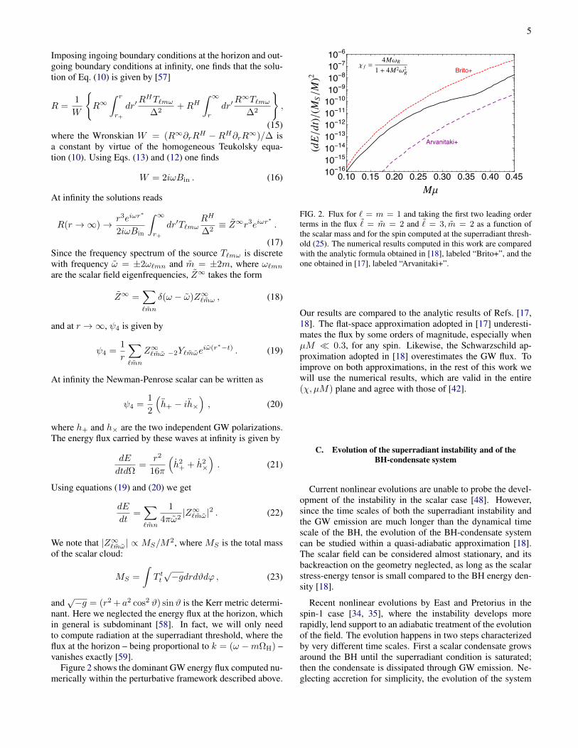
Figure 2 shows the dominant GW energy flux computed nu-merically within the perturbative framework described above.

-----------

+

+

FIG. 2. Flux for ` = m = 1 and taking the first two leading orderterms in the flux ˜ = m = 2 and ˜ = 3, m = 2 as a function ofthe scalar mass and for the spin computed at the superradiant thresh-old (25). The numerical results computed in this work are comparedwith the analytic formula obtained in [18], labeled “Brito+”, and theone obtained in [17], labeled “Arvanitaki+”.

Our results are compared to the analytic results of Refs. [17,18]. The flat-space approximation adopted in [17] underesti-mates the flux by some orders of magnitude, especially whenµM 0.3, for any spin. Likewise, the Schwarzschild ap-proximation adopted in [18] overestimates the GW flux. Toimprove on both approximations, in the rest of this work wewill use the numerical results, which are valid in the entire(χ, µM) plane and agree with those of [42].

C. Evolution of the superradiant instability and of theBH-condensate system

Current nonlinear evolutions are unable to probe the devel-opment of the instability in the scalar case [48]. However,since the time scales of both the superradiant instability andthe GW emission are much longer than the dynamical timescale of the BH, the evolution of the BH-condensate systemcan be studied within a quasi-adiabatic approximation [18].The scalar field can be considered almost stationary, and itsbackreaction on the geometry neglected, as long as the scalarstress-energy tensor is small compared to the BH energy den-sity [18].

Recent nonlinear evolutions by East and Pretorius in thespin-1 case [34, 35], where the instability develops morerapidly, lend support to an adiabatic treatment of the evolutionof the field. The evolution happens in two steps characterizedby very different time scales. First a scalar condensate growsaround the BH until the superradiant condition is saturated;then the condensate is dissipated through GW emission. Ne-glecting accretion for simplicity, the evolution of the system

6

is governed by the equations [18]M = −ES ,M + MS = −E ,J = −mES/ωR ,J + JS = −mE/ωR ,

(24)

where ES = 2MSωI is the scalar energy flux extracted fromthe horizon through superradiance. In the above equations,we have used the fact that – for a single (`, m) mode – theGW angular momentum flux is mE/ωR and that the angularmomentum flux of the scalar field extracted at the horizon ismES/ωR.

The system (24) shows that for a superradiantly unstablestate (ωI > 0) the instability will cause the BH to transfermass and spin to the scalar field until the system reaches thesaturation point, given by ωI = 0, i.e., ωR = mΩH.2 Thisprocess occurs on a time scale τinst ≡ 1/ωI M , and thesaturation point corresponds a final BH angular momentum

Jf =4mM3

fωR

m2 + 4M2fω

2R

< Ji , (25)

where Ji/f , Mi/f are the initial/final BH angular momentumand mass, respectively. The system (24) also shows that thevariation of the BH mass δM is related to the variation of theBH angular momentum δJ by δM = ωR

m δJ , which implies

Mf = Mi −ωRm

(Ji − Jf ) . (26)

When the instability saturates, the total mass of the scalarcloud is roughly given by Mmax

S ∼Mi −Mf , namely

MmaxS ∼ JiωR

m−

4M3fω

2R

m2 + 4M2fω

2R

≈ JiωRm

, (27)

where the last step is valid when MfωR 1.After the superradiant phase, the mass and the angular mo-

mentum of the BH remain constant [cf. Eq. (24)], whereasthe scalar field is dissipated through the emission of GWs3

as given by Eq. (22). We neglect GW absorption at the eventhorizon – which is always sub-dominant [58] – and GW emis-sion due to the transition of bosons between different energylevels, which is also a sub-dominant effect as long as the con-densate is mostly populated by a single level [19]. By usingagain Eq. (24), after the superradiant phase we get

MS = −dEdt

= −dEdt

M2S

M2f

, (28)

2 Fully non-linear evolutions of a charged scalar field around a charged BHenclosed by a reflecting mirror [50, 60, 61] or in anti-de Sitter space-time [51] have shown that the end-state for this system indeed consists ofa scalar condensate around a charged BH saturating the superradiant con-dition. East and Pretorius reached the same conclusion for massive spin-1fields [34, 35]. For complex fields, truly stationary metric solutions of thefield equations describing a boson condensate saturating the superradiantcondition around spinning BH have been explicitly shown to exist [62–64]

3 In the language of [19] this process corresponds to the “axion+axion →graviton” annihilation process. In our notation, their “occupation number”is N =MS/ms.

where we used the fact that |Z∞`mω|2 ∝ M2S to factor out the

dependence on MS(t), and we defined dEdt ≡

dEdt

M2f

M2S

. Thisquantity is shown in Figure 2 and it is constant after the su-perradiant phase, since it depends only on the final BH massand spin. Therefore, setting t = 0 to be the time at which thesuperradiant phase saturates, the above equation yields

MS(t) =MmaxS

1 + t/τGW, (29)

where MmaxS is the mass of the condensate at the end of the

superradiant phase [cf. Eq. (27)] and

τGW ≈Mf

(dE

dt

MmaxS

Mf

)−1

≈ 8× 105 yr

[Mf

106M

] [10−11

dE/dt

] [0.2Mf

MmaxS

](30)

is the gravitational radiation time scale.Finally, we note that the self-gravity of the boson cloud will

cause the GW frequency to change slightly as the cloud dis-sipates via GWs [19, 21]. The estimates of Refs. [19] [seetheir Eq. (28)] and [21] [see their Appendix E] suggest that,for scalar fields, this small change should not affect currentcontinuous-wave searches. Taking these estimates and theduration of the signal of Figs. 3 and 4 for resolved events,one can see that for both LIGO and LISA a vast major-ity of the sources will have a small positive frequency driftf 10−9Hz/s, which is the current upper limit on thefrequency time derivative of the latest all-sky search fromLIGO [65]. However, even though this frequency drift shouldbe very small and undetectable for most sources, the positivefrequency time derivative of GWs from boson clouds could beused to distinguish them from other continuous sources, suchas rotating neutron stars, which have a negative frequencydrift [66].

D. Instability and gravitational radiation time scales

As discussed above, the basic features of the evolution ofthe BH superradiant instability in the presence of light bosonscan be understood as a two-step process, governed by two dif-ferent time scales. The first time scale is the typical e-foldingtime of the superradiant instability given by τinst ≡ 1/ωI ,where in the Mµ 1 limit, ωI is the imaginary part ofEq. (8). The boson condensate grows over the time scale τinst

until the superradiant condition is saturated. Subsequently,the condensate is dissipated through GW emission over a timescale τGW given by Eq. (30). In the Mµ 1 limit, dE/dt =(484 + 9π2)/23040(µM)14 ' 0.025(µM)14 [18, 42]. Thus,using Eqs. (8), (27), (30) and reinstating physical units, thetwo most relevant time scales of the system are of the order

τinst ∼ 105yr(M8

6µ917χ)−1

, (31)

τGW ∼ 5× 1011yr(M14

6 µ1517χ)−1

, (32)

7

----

----

----

--------

FIG. 3. Gravitational radiation time scale, instability time scale, and the signal duration ∆t [defined in Eq. (33)] for detectable LISA sourcesand for different boson masses.

where M6 = M/(106M) and µ17 = ms/(10−17eV) andχ 1.

These relations are still a reasonably good approximationwhen Mµ ∼ 1 and χ ∼ 1. They show that there is a clearhierarchy of time scales (τGW τinst M ), and this isimportant for two reasons. First of all it is crucial that τGW τinst, otherwise the boson condensate would not have time togrow. Second, the time scale hierarchy justifies the use of anadiabatic approximation to describe the evolution.

Beyond the instability and gravitational radiation timescales, from the point of view of detection it is important toestimate the distribution of signal durations ∆t. For LIGOwe can safely neglect accretion, because accreted matter isnot expected to significantly alter the birth spin of stellar-massBHs [67]. We can also neglect the effect of mergers, sincemergers affect a very small fraction of the overall populationof isolated BHs [68–72], and LIGO data already suggest thatmultiple mergers should be unlikely [73, 74]. Therefore, forLIGO we will simply assume ∆t = min (τGW, t0), wheret0 ≈ 13.8 Gyr is the age of the Universe.

For massive BHs that radiate in the LISA band, both merg-ers and accretion are expected to be important [75, 76]. There-fore we conservatively assume that whenever an accretionevent or a merger happens the boson-condensate signal is cut

short, and for LISA we define

∆t =

⟨min

(τGW

Nm + 1, tS , t0

)⟩, (33)

where the signal duration τGW in the absence of mergersand accretion is given by Eq. (30), 〈...〉 denotes an aver-age weighted by the probability distribution function of theEddington ratios, tS is the “Salpeter” accretion time scale[Eq. (51)], and Nm is the average number of mergers ex-pected in the interval [t − τGW/2, t + τGW/2], t being thecosmic time corresponding to the cosmological redshift z ofthe GW source. Note that this definition also enforces theobvious fact that the signal cannot last longer than the ageof the Universe (∆t ≤ t0). We also note that the estimatesof Refs. [19, 21] suggest that the close passage of a stellar-mass compact object around the massive BH could affect theboson cloud when Mµ 0.1. This part of the parameterspace is mostly irrelevant for our results, and so we neglectthis contribution. Moreover, estimates of the rates of extrememass-ratio inspirals predict at most a few hundred such closepassages per Gyr per galaxy [46]. Therefore, the averagetimescale between these events is & 107 yr. This is compa-rable with the accretion timescale [Eq. (51)], which we havealready taken into account. Thus, we expect our results to berobust against inclusion of this effect. In addition, stars and

8

- - ----

- - ----

- - ----

- - ----

FIG. 4. Gravitational radiation time scale, instability time scale, and the signal duration ∆t [defined in Eq. (33)] for detectable LIGO sourcesand for different boson masses. Dashed lines represent extragalactic sources and bold lines represent Galactic sources.

compact objects could, in principle, affect the boson cloudalso at larger orbital distances, comparable to the peak of thecloud R ∼ 4M/(Mµ)2 [18]. This could also become rele-vant for Mµ 0.1, but even in this case passages of stars atR ∼ 1000M or larger are expected to be quite rare. Indeed,tidal disruption of stars are about 10−5 per yr per galaxy [77],hence stars at distancesR ∼ 1000M from the BH should onlyappear roughly every 105 yr. We have checked that even if weinclude this effect by adding an extra timescale ∼ 105 yr toEq. (33), the background and the resolved event rates wouldonly decrease by about an order of magnitude (and only forMµ 0.1), thus leaving our conclusions unchanged.

Figures 3 and 4 show histograms of τinst, τGW and ∆t forresolvable sources with SNR ρ ≥ 8 [cf. Eq. (34)]. Whencomputing the SNR, we use an observation time Tobs = 2 yrfor LIGO and Tobs = 4 yr for LISA. We adopt the LISA noisepower spectral density specified in the ESA proposal for L3mission concepts [11] and the design sensitivity of AdvancedLIGO [78]. The events are binned by gravitational radiationtime scale τGW, instability time scale τinst, and signal dura-tion ∆t, as defined in Eq. (33). For concreteness, in the plotwe focus on the most optimistic astrophysical model, and weneglect the confusion noise due to the stochastic backgroundproduced by these sources [cf. [79]]. For LIGO we show bothGalactic and extragalactic sources.

The signal duration ∆t is typically equal to the gravitationalradiation time scale τGW, and (as anticipated) much longerthan the instability time scale τinst. Since for LIGO we ne-glect the effects of mergers and accretion, the only visible dif-ference between ∆t and τGW is due to the fact that we cut offthe signal when its typical time scale is longer than the ageof the Universe (i.e., as mentioned above, we set ∆t = t0 ifτGW > t0). For LISA there are more subtle effects related toaccretion and mergers [cf. Eq. (33)], but Figs. 3 and 4 demon-strate that the signal duration ∆t is always much longer thanthe instability time scale τinst, as suggested by the rough esti-mates of Eqs. (31) and (32).

E. Gravitational waveform

Since the GW signal from boson condensates is quasi-monochromatic, we can can compute the (average) signal-to-noise ratio (SNR) as [80, 81]

ρ '

⟨h√Toverlap√Sh(f)

⟩, (34)

where h is the root-mean-square (rms) strain amplitude;Sh(f) is the noise power spectral density at the (detector-frame) frequency f of the signal, which is related to the

9

source-frame frequency fs ≡ ω/(2π) by f = fs/(1 + z)(z being the redshift); Toverlap is the overlap time between theobservation period Tobs and the signal duration ∆t(1 + z) [inthe detector frame, hence the factor 1 + z multiplying the sig-nal duration ∆t in the source frame]; and 〈. . . 〉 denotes anaverage over the possible overlap times. In practice, when ourastrophysical models predict that a signal should overlap withthe observation window, we compute this average by random-izing the signal’s starting time with uniform probability distri-bution in the interval [−∆t(1 + z), Tobs] (where we assume,without loss of generality, that t = 0 is the starting time of theobservation period).

Coherent searches for almost-monochromatic sources arecomputationally expensive, and normally only feasible whenthe intrinsic parameters of the source and its sky location areknown. For all-sky searches, where the properties and loca-tion of the sources are typically unknown, it is more commonto use semicoherent methods, where the signal is divided inN coherent segments with time length Tcoh. The typical sen-sitivity threshold, for signals of duration ∆t(1 + z) Tobs,is [cf. e.g. [66]]

hthr '25

N 1/4

√Sh(f)

Tcoh, (35)

where hthr is the minimum rms strain amplitude detectableover the observation time N × Tcoh. This criterion was used,for example, in [19]. In the following we consider both cases(a full coherent search and a semicoherent method) in order tobracket uncertainties due to specific data analysis choices. Forthe semicoherent searches we only consider events for which∆t(1 + z) Tobs [since the threshold gived by eq. (35) onlyholds for long-lived signals].

A useful quantity to compare the sensitivity of differentsearches independently of the data-analysis technique and thequality and amount of data is the so-called “sensitivity depth,”defined by [82]

D(f) =

√Sh(f)

hthr. (36)

For example, the average sensitivity depth of the last EIN-STEIN@HOME search was D ≈ 35Hz−1/2 [83].

To compute h, we first use Eqs. (9), (19) and (20) to get acombination of the two GW polarizations,

H ≡ h+− ih× = − 2

ω2r

∑`mn

Z∞`mω −2Y`mωeiω(r∗−t) . (37)

In the following we will omit the sum over `mn for easeof notation. Let us focus on a single scalar field mode4. Ifthe scalar field has azimuthal number m and real frequencyωR, the GW emitted by the scalar cloud will have azimuthal

4 In this work we will focus on the mode with the smallest instability timescale ` = m = 1, which should be the dominant source of GW radia-tion [19].

number m = ±2m and frequency ω = ±2ωR. DefiningZ∞ = |Z|e−iφ, where |Z| and φ are both real, we have

H = −2|Z|ω2r

(−2Y`mωe

i[ω(r∗−t)+φ]

+−2Y`−m−ωe−i[ω(r∗−t)+φ]

), (38)

where we used the fact that Z∞`−m−ω = Z∞`mω . SincesY`mω(ϑ, ϕ) = sS`mω(ϑ)eimϕ and S is a real function forreal ω, we get

h+ = <(H) ≡− 2|Z|ω2r

(−2S`mω + −2S`−m−ω)

× cos [ω(r∗ − t) + φ+ mϕ] , (39)

h× = =(H) ≡− 2|Z|ω2r

(−2S`mω − −2S`−m−ω)

× sin [ω(r∗ − t) + φ+ mϕ] . (40)

The GW strain measured at the detector is

h = h+F+ + h×F× , (41)

where F+,× are pattern functions that depend on the orienta-tion of the detector and the direction of the source. To get therms strain of the signal we angle-average over source and de-tector directions and use

⟨F 2

+

⟩=⟨F 2×⟩

= 1/5, 〈F+F×〉 = 0,⟨|sS`mω|2

⟩= 1/(4π) and

⟨cos2 [ω(r∗ − t) + φ+ mϕ]

⟩=⟨

sin2 [ω(r∗ − t) + φ+ mϕ]⟩

= 1/2. We then obtain

h '⟨h2⟩1/2

=

(2|Z|2

5πω4r2

)1/2

=

(4E

5ω2r2

)1/2

, (42)

where E is given in Eq. (22), which for a single scalar modereads E =

∑` |Z`|2/(2πω2). Finally, let us factor out the

BH mass and the mass of the scalar condensate: |Z| =A(χ, µM)(Mω)2MS/M

2, where A(χ, µM) is a dimension-less quantity. The final expression for the rms strain reads

h =

√2

5π

M

r

MS

MA(χ, µM) . (43)

We conservatively assume that the GWs observed at the detec-tor are entirely produced after the saturation phase of the insta-bility. Therefore, we compute h using the final BH mass andspin, as computed in Eqs. (26) and (25), respectively. Largerinitial spins imply that a larger fraction of the BH mass istransferred to the scalar condensate [cf. Eq. (27)]. So, for agiven scalar field mass and initial BH mass, the strain growswith the initial spin.

Equation (43) is valid for any interferometric detector forwhich the arms form a 90-degree angle, such as AdvancedLIGO. For a triangular LISA-like detector the arms form a60-degree angle, and we must multiply all amplitudes by a ge-ometrical correction factor

√3/2 [5, 84]. Additionally, since

we sky-average the signal, we will use an effective non-sky-averaged noise power spectral density, obtained by multiply-ing LISA’s sky-averaged Sh by 3/20 [85]. The analysis pre-sented below takes into account these corrective factors.

10

- - - - --

- - - - --

- - - --

-

- - - --

-

FIG. 5. Angle-averaged range Drange for LISA (top) and Advanced LIGO at design sensitivity (bottom) computed for selected initial BH spin(χi = 0.998, 0.95, 0.7). Left panels: the range is computed using a coherent search over an observation time Tobs = 4 yr (for LISA) andTobs = 2 yr (for LIGO). Right panels: we assume a semicoherent search withN = 121 coherent segments of duration Tcoh = 250 hr.

F. Cosmological effects

Since some sources can be located at non-negligible red-shifts, the root-mean-square strain amplitude of Eqs. (42)and (43) must be corrected to take into account cosmologi-cal effects, which affect the propagation of the waves to thedetector [86]. These effects have two main consequences.

First, the frequency f of the signal as measured at thedetector’s location (“detector frame”) is redshifted with re-spect to the emission frequency fs in the “source-frame”, i.e.f = fs/(1 + z).

Second, in the strain amplitude given by Eq. (43), the dis-tance r to the detector should be interpreted as the comov-ing distance, which for a flat Friedmann-Lemaitre-Robertson-Walker model is given by

Dc(z) = DH

∫ z

0

dz′√∆(z′)

, (44)

where ∆(z) = ΩM (1+z)3 +ΩΛ, DH is the Hubble distance,ΩM is the dimensionless matter density and ΩΛ is the dimen-sionless cosmological constant density. All other quantities

(masses, lengths and frequencies) in Eq. (43) should be in-stead be interpreted as measured by an observer in the sourceframe.

Alternatively, one might wish to use quantities measuredby an observer at the detector’s location to compute the strainamplitude of Eq. (43). Detector-frame quantities are relatedto source-frame ones by powers of (1 + z), namely all quan-tities with dimensions [mass]p (in our geometrized units G =c = 1) are multiplied by the factor (1 + z)p, e.g. masses aremultiplied by (1 + z) (“redshifted masses”), frequencies aredivided by the same factor (“redshifted frequencies”), whilethe comoving distance is multiplied by a factor (1 + z), thusbecoming the luminosity distanceDL = Dc(1+z). Since thestrain amplitude of Eq. (43) is dimensionless, that equationyields the same result when using detector-frame quantities aswhen using source-frame ones.

The typical distance up to which BH-condensate sourcesare detectable can be estimated by defining an “angle-averaged range” Drange as the luminosity distance at whicheither the SNR ρ(Drange) = 8 [cf. Eq. (34)] for coherentsearches, or h(Drange) = hthr for semicoherent searches [cf.

11

Eq. (35)].In Fig. 5 we show Drange for both LISA and LIGO at de-

sign sensitivity under different assumptions on the initial BHspin. The left panels refer to single coherent observation withTobs = 4 yr for LISA (Tobs = 2 yr for Advanced LIGO),whereas the right panels refer to a (presumably more realistic)semicoherent search with N = 121 coherent segments of du-ration Tcoh = 250 hr. In the more optimistic case, sourcesare detectable up to cosmological distances of ∼ 20 Gpc(∼ 2 Gpc) if the BH is nearly extremal and the boson mass isin the optimal mass range ms ∼ 10−17 eV (ms ∼ 10−13 eV)for LISA (LIGO). For the semicoherent search, Drange is re-duced by roughly one order of magnitude, with a maximumdetector reach ∼ 2 Gpc and ∼ 200 Mpc for LISA and Ad-vanced LIGO, respectively.

III. MASSIVE BLACK HOLE POPULATION MODELS

An assessment of the detectability of GWs from superra-diant instabilities requires astrophysical models for the mas-sive BH population. In this section we describe the modelsadopted in our study, and in particular our assumptions on (A)the mass and spin distribution of isolated massive BHs, (B)their Eddington ratio distribution, and (C) their merger his-tory.

A. Mass and spin distribution of isolated black holes

Let n be the comoving-volume number density of BHs. Forthe mass and spin distribution of isolated BHs we consider:

(A.1) A model where d2n/(d log10Mdχ) is computed usingthe semianalytic galaxy formation model of [43] (withlater improvements described in [76, 87, 88]). This dis-tribution is redshift-dependent and skewed toward largespins, at least at low masses (cf. [76]). It also has anegative slope dn/d log10M ∝ M−0.3 for BH massesM < 107M, which is compatible with observations(cf. [76], Figure 7). The normalization is calibrated soas to reproduce the observed M–σ and M–M? scalingrelations of [89], where σ is the galaxy velocity disper-sion and M? is the stellar mass. We also account for thebias due to the resolvability of the BH sphere of influ-ence [90, 91]. Because of the slope, normalization andspin distribution, this model is optimistic.

(A.2) An analytic mass function [46, 47]

dn

d log10M= 0.005

(M

3× 106M

)−0.3

Mpc−3, (45)

which we use for redshifts and BH masses in the range104M < M < 107M and z < 3. For M > 107Mwe use a mass distribution with normalization 10 timeslower than the optimistic one. For this model we use auniform distribution of the initial spins χ ∈ [0, 1]. Be-cause of the lower normalization and the spin distribu-tion, this model is less optimistic.

(A.3) An analytic mass function

dn

d log10M= 0.002

(M

3× 106M

)0.3

Mpc−3, (46)

which we use again for 104M < M < 107M andz < 3, whereas for M > 107M we use a mass dis-tribution with normalization 100 times lower than theoptimistic one. For this model we also consider a uni-form distribution of the initial spins χ ∈ [0, 1]. Becauseof the normalization, slope and spin distribution, thismodel is pessimistic.

B. Black hole mergers

Our standard choice for BH mergers is to compute thecomoving-volume number density nm of mergers per (loga-rithmic) unit of total mass Mtot = M1 + M2, unit redshiftand (logarithmic) unit of mass ratio q = M2/M1 ≤ 1, i.e.

ν(Mtot, z, q) ≡d3nm

d log10Mtotdzd log10 q, (47)

from the semianalytic model of [43].We can then estimate the average number of mergers (be-

tween z and z + dz) for a BH of mass M as

dNm(M, z) =µ(M, z)

φ(M, z)dz . (48)

Here

φ(M, z) ≡ dn

d log10M=

∫d2n

d log10Mdχdχ (49)

is the (isolated BH) mass function, and

µ(Mtot, z) ≡d2nmerger

d log10Mtotdz=

∫q>qc

ν d log10 q ,

where qc is the critical mass ratio above which we assumemergers make an impact. In practice, most BH mergers in oursemianalytic models have q & 0.01–0.001 (especially in theLISA band, cf. [92]), so our results are robust against the exactchoice of qc. Nevertheless, to be on the conservative side,we set qc = 0. A larger qc would produce a slightly lowerBH merger number and, in turn, a slightly higher number ofboson-condensate sources, under the conservative assumptionthat mergers destroy the boson cloud. We can then computethe average number of mergers experienced by a BH of massM in the redshift interval [z1, z2] as

Nm =

∫ z2

z1

dNmdz

dz . (50)

Note that the number of mergers depends on the seedingmechanisms of the massive BH population, as well as on the

12

“delays” between the mergers of galaxies and the mergers ofthe BHs they host [cf. e.g. [39]].

When computing the average number of mergers Nm tobe used to estimate the number of boson-condensate GWevents from isolated BHs, i.e. when evaluating the num-ber of resolved events [Eq. (62) below] and the amplitudeof the stochastic background [Eq. (64) below], we considerthe “popIII” model of [39] (a light-seed scenario with delays).Choosing a different seed model would not alter our conclu-sions. However, when considering the constraints that can beplaced on the boson mass by direct observations of BH co-alescences by LISA, we consider all three models presentedin [39] (“popIII”, “Q3” and “Q3nod”). These models corre-spond respectively to light seeds with delays between a galaxymerger and the corresponding binary BH merger; heavy seedswith delays; and heavy seeds with no delays; and they are cho-sen to bracket the theoretical uncertainties on the astrophysicsof BH seed formation and BH delays.

C. Accretion

Clearly, accretion is competitive with the superradiant ex-traction of angular momentum from the BH [18], so it is im-portant to quantify its effect. We estimate the accretion timescale via the Salpeter time,

tS = 4.5× 108 yrη

fEdd(1− η), (51)

where fEdd is the Eddington ratio for mass accretion, and thethin-disk radiative efficiency η is a function of the spin relatedto the specific energy E

ISCOat the innermost stable circular

orbit [93]:

η = 1− EISCO

, (52)

EISCO

=

√1− 2

3rISCO

, (53)

rISCO

= 3 + Z2 −χ

|χ|√

(3− Z1)(3 + Z1 + 2Z2) , (54)

Z1 = 1 + (1− χ2)1/3[(1 + χ)1/3 + (1− χ)1/3

], (55)

Z2 =√

3χ2 + Z21 . (56)

For the Eddington ratio fEdd we consider three models:

(C.1) We use the results of our semianalytic model to con-struct probability distribution functions for fEdd at dif-ferent redshifts and BH masses.

(C.2) We adopt a simple model in which fEdd = 1 for 10%of the massive BHs, and fEdd = 0 for the remainingones. (The choice of 10% is a reasonable estimate forthe duty cycle of active galactic nuclei [94, 95]).

(C.3) Finally, we consider a very pessimistic model in whichall BHs have fEdd = 1. Although unrealistic, this mod-els maximizes the effects of accretion, and therefore ityields the most conservative lower bound for the super-radiant instability time scale.

IV. STELLAR MASS BLACK HOLE POPULATIONMODELS

We now turn to a description of stellar-mass BHs, which areof interest for LIGO. Here we have to model (A) extragalacticBHs, which turn out to dominate the stochastic background ofGWs from ultralight bosons, and (B) Galactic BHs, which (aspointed out in [19, 20]) are dominant in terms of resolvablesignals.

A. Extragalactic BHs

In the standard scenario, stellar-mass BHs are the end prod-ucts of the evolution of massive (M & 20M) stars. Theyform either via direct collapse of the star or via a supernovaexplosion followed by fallback of matter (failed supernova).This process depends on various parameters, such as stellarmetallicity, rotation and interactions with a companion if thestar belongs to a binary system [96–99]. In particular, themetallicity of the star determines the strength of stellar windsand can thus have a significant impact on the mass of the stel-lar core prior to collapse [100, 101]. In addition, BHs cangrow hierarchically through multiple mergers that occur indense stellar clusters [73, 74, 102, 103]. This process is ex-pected to leave an imprint on the distribution in the mass-spinplane: while BHs grow in mass via mergers their spins con-verge to values around ∼ 0.7 with little or no support below∼ 0.5 [73–75].

In this work we consider only BH formation from corecollapse of massive stars. We use the analytic fits for theBH mass as a function of initial stellar mass and metallicityfrom [104], embedded in the semianalytic galaxy evolutionmodel from [105]. In particular, the latter model describes theproduction of metals by stars [106] and the evolution of themetallicity of the interstellar medium, which is inherited bythe stars that form there. The extragalactic BH formation rateas a function of mass and redshift readsdneg

dM=

∫dM?ψ[t− τ(M?)]φ(M?)δ[M? − g−1(M)] ,

(57)where τ(M?) is the lifetime of a star with massM?, φ(M?)is the stellar initial mass function, ψ(t) denotes the cosmicstar formation rate (SFR) density and δ is the Dirac delta. Weuse the fit to the cosmic SFR described in [107], calibratedto observations [108, 109]. We adopt a Salpeter initial massfunction φ(M?) ∝ M?

−2.35 [110] in the mass rangeM? ∈[0.1 − 100]M and use the stellar lifetimes from [111]. Theinitial stellar mass M? and BH mass M are related by thefunction M = g(M?), which can be (implicitly) redshift-dependent (through its dependence on stellar metallicity), andwhich we take from the “delayed” model of [104].

B. Galactic BHs

Resolvable signals are expected to be dominated by Galac-tic stellar-mass BHs [19]. We estimate the present-day mass

13

function of these BHs as

dNMW

dM=

∫dt

SFR(z)

M?

dp

dM?

∣∣∣∣ dMdM?

∣∣∣∣−1

, (58)

where NMW denotes the number of BHs in the Galaxy,dp/dM? is the normalized Salpeter initial mass function (i.e.the probability of forming a star with mass betweenM? andM? + dM?), and SFR(z) denotes the SFR of Milky-Waytype galaxies as a function of z [109, 112]. The integrationis over all cosmic times till the present epoch. The (dif-ferential) relation between BH mass and initial stellar massdM/dM? is taken from the “delayed” model of [104], andis also a function of redshift via the metallicity. For the lat-ter, we use the results of [113] to describe its evolution withcosmic time. We then “spread” dNMW/dM throughout theGalaxy in order to obtain a (differential) density dnMW/dM ,by assuming that the latter is everywhere proportional to the(present) stellar density. To this purpose, we describe theGalaxy by a bulge+disk model, where the bulge follows aHernquist profile [114] with mass ∼ 2 × 1010M and scaleradius ∼ 1 kpc [115], and the disk is described by an expo-nential profile with mass ∼ 6× 1010M and scale radius ∼ 2kpc [116].

Since these models (for both Galactic and extragalacticBHs) do not predict the initial BH spins, we assume a uniformdistribution and explore different ranges (from optimistic topessimistic): χ ∈ [0.8, 1], [0.5, 1], [0, 1] and [0, 0.5].

V. EVENT RATES FOR LISA AND LIGO

Having in hand the calculation of the GW signal of Sec. IIand the astrophysical models of Secs. III and IV, we can nowcompute event rates for LISA and LIGO. We consider twoseparate classes of sources: (A) boson-condensate GW eventswhich are loud enough to be individually resolvable, and (B)the stochastic background of unresolvable sources.

A. Resolvable sources

In the limit in which the (detector-frame) signal duration∆t(1 + z) is small compared to the observation time Tobs,∆t(1 + z) Tobs, the number of resolvable events is propor-tional to the observation time [117]:

N = Tobs

∫ρ>8

d2n

dMdχ

dt

dz4πD2

cdzdMdχ , (59)

where

dt

dz=

1

H0

√∆(1 + z)

(60)

is the derivative of the lookback time with respect to redshift.For long-lived sources with detector-frame duration ∆t(1+

z) Tobs, the number of detections does not scale withthe observation time, but rather with the “duty cyle” ∆t/tf ,

where tf ≡ n/n is the formation time scale of the bosoncondensate. For example, if BHs form a boson condensateonly once in their cosmic history, tf is the age of the Uni-verse t0 ≈ 13.8 Gyr. This duty cycle has the same meaningas the duty cycle of active galactic nuclei: it accounts for thefact that, at any given time, only a fraction of the BH popu-lation will be emitting GWs via boson condensates. Becauseof the ergodic theorem, this fraction is given by the averagetime fraction during which a BH emits GWs via boson con-densates. This average time fraction is indeed the duty cy-cle ∆t/tf . Therefore, the number of resolved sources when∆t(1 + z) Tobs is simply

N =

∫ρ>8

d2n

dMdχ

∆t

tf

dVcdz

dzdMdχ

=

∫ρ>8

d2n

dMdχ∆t

dVcdz

dzdMdχ , (61)

where dVc = 4πD2cdDc.

Equations (59) and (61) can be merged into a single ex-pression that remains valid also in the intermediate regime∆t(1+z) ∼ Tobs. Indeed, the probability that a signal lastinga time span ∆t(1+z) (in the detector frame) overlaps with anobservation of duration Tobs is simply proportional to the sumof the two durations, ∆t(1+z)+Tobs. This can be understoodin simple geometric terms: for the signal to overlap with theobservation window (which we define, without loss of gener-ality, to extend from t = 0 to t = Tobs), the signal’s startingtime should fall between t = −∆t(1 + z) and t = Tobs, i.e.in a time interval of length ∆t(1 + z) + Tobs. Therefore, wecan estimate the number of observable GW events as

N =

∫ρ>8

d2n

dMdχ

(Tobs

1 + z+ ∆t

)dVcdz

dzdMdχ . (62)

Since dDc/dz = (1 + z)dt/dz, it can be easily checked thisequation reduces to Eqs. (59) and (61) in the limits ∆t(1 +z) Tobs and ∆t(1 + z) Tobs, respectively.

For extragalactic LIGO sources we compute d2n/dMdχfrom the astrophysical models of Sec. IV A, while for LISAand galactic LIGO sources we compute d2n/dMdχ as de-scribed in Secs. III and IV B and then assume d2n/dMdχ =(d2n/dMdχ)/t0. This corresponds to assuming that theboson-condensate formation time tf = t0 equals the age ofthe Universe, or that BHs radiate via boson condensates onlyonce in their lifetime. This conservative assumption does notaffect our results very significantly. Once a BH-boson sys-tem radiates, its spin decreases to low values, while the massremains almost unchanged. For the BH to emit again via bo-son condensates, its spin must grow again under the effectof accretion or mergers. In this process, however, the BHmass also grows rapidly: for example, the simple classic esti-mates by Bardeen [118] imply that when a BH spins up fromχ = 0 to χ = 1 via accretion, its mass increases by a factor√

6. So even if new boson clouds form due to the instabilityof higher-m modes, the instability time scales will be muchlarger [cf. Eq. (8)] and the GW flux will be highly suppressed[cf. Ref. [42]].

14

- - - - - - - - ---

FIG. 6. Number of resolved LIGO and LISA events for our opti-mistic BH population models as a function of the boson mass withdifferent observation times Tobs, using both full and semicoherentsearches. Thick (thin) lines were computed with (without) the con-fusion noise from the stochastic background.

Our main results for resolvable rates are summarized inFig. 6, Fig. 7, Table I and Table II.

In Fig. 6 we focus on optimistic models and we show howthe number of individually resolvable events depends on theobservation time and on the chosen data-analysis method.More specifically, for LISA we use the BH mass-spin dis-tribution model (A.1) and accretion model (C.1), while forLIGO we adopt the optimistic spin distribution χi ∈ [0.8, 1].We bracket uncertainties around the nominal LISA missionduration of Tobs = 4 yr [11] by considering single obser-vations with duration Tobs = (2, 4, 10) yr. We also showrates for a (presumably more realistic) semicoherent searchwith 121 segments of Tcoh = 250 hours coherent integrationtime5. For Advanced LIGO at design sensitivity, we simi-larly consider single observations lasting either Tobs = 2 yror Tobs = 4 yr, as well as a semicoherent search with 121segments of Tcoh = 250 hours coherent integration time.

Figure 6 (together with Figure 3 in [79]) shows that thenumber of resolvable events is strongly dependent on the bo-son mass and on the astrophysical model.

For LISA, our astrophysical populations contain mostlyBHs in the mass range 104M < M < 108M, and thesensitivity curve peaks around a frequency corresponding toms ∼ 10−17eV [cf. Fig. 1 of [79]]. These considerations –together with the condition for having an efficient superradi-ant instability (namely, Mµ ∼ 0.4 at large spin) – translateinto the range 3 × 10−18 eV . ms . 5 × 10−17 eV for themass of detectable bosonic particles in a semicoherent search.

For LIGO, our models predict that most BHs will be in themass range 3M < M < 50M, and the most sensitivefrequency band corresponds to ms ∼ 3× 10−13eV [cf. Fig. 1

5 The number of resolved events for other choices of number of segmentsand coherent integration time can be obtained from Fig. 7 and expressingthe sensitivity depth as D ≈ T 1/2

cohN1/425−1 [cf. Eqs. (35) and (36)].

of [79]], translating into the range 2 × 10−13 eV . ms .3× 10−12 eV for the mass of detectable bosonic particles.

In order to quantify the “self-confusion” noise due to thestochastic background produced by BH-boson systems, inFig. 6 we also display the number of resolved events thatwe would obtain if we omitted the confusion noise from thestochastic background (cf. Fig. 1 of [79] and Sec. V B). Ne-glecting the confusion noise would overestimate the numberof resolvable events in LISA by one or two orders of magni-tude.

The rates computed in Figure 6 refer to our optimistic as-trophysical models. As shown in [79], resolvable event ratesin the most pessimistic models are about one order of mag-nitude lower. Nevertheless, it is remarkable that even inthe most pessimistic scenario for direct detection (i.e., unfa-vorable BH mass-spin distributions and semicoherent searchmethod for the signal), bosonic particles withms ∼ 10−17 eV(ms ∼ 10−12 eV) would still produce around 5 (15) directLISA (LIGO) detections of boson-condensate GW events.

In Figure 7 we show how the number of events grows withthe sensitivity depth of the search [82], as defined in Eq. (36).For LISA the number of events grows roughly with D3, cor-responding to T 3/2

obs . This is expected from the fact that thenumber of events for sources at & 30 Mpc should grow withthe sensitive volume, and thus decrease with ρ−3

crit, where ρcrit

is the critical SNR for detection [119].On the other hand, LIGO will be mostly sensitive to sig-

nals within the Galaxy. For a given boson mass and distance,τGW ∼ h−2 andM ∼ h1/8 [cf. Eqs. (30) and (42)]. Since theGalactic stellar BH population obtained from Eq. (58) is wellfitted by dN/M ∼ e−0.2M , for a fixed volume the integral inEq. (61) goes as

N ∼∫h>hthr

h−23/8e−0.2h1/8

dh ∼ h−15/8thr , (63)

where in the last step we took the leading order of the integralfor small hthr. From Eq. (34) one has hthr ∝ T

−1/2obs and

therefore N ∝ T15/16obs . This is in agreement with the scaling

that we find.Assuming the sensitivity depth of the last EIN-

STEIN@HOME search D ≈ 35Hz−1/2 [83] and an optimalboson mass around ms ∼ 10−12.5 eV, we find that O1should have detected 5 resolvable events for the optimisticspin distribution χ ∈ [0.8, 1], and 2 events for a uniformspin distribution χ ∈ [0, 1]. As pointed out in [79], theseoptimal boson masses may already be ruled out by upperlimits from existing stochastic background searches [79]. Onthe other hand, the pessimistic spin distribution χ ∈ [0, 0.5]is still consistent with (the lack of) observations of resolvableBH-boson GW events in O1, though marginally ruled out bythe O1 stochastic background upper limits [79].

Our results for resolvable event rates using different searchtechniques, mass/spin and accretion models are summarizedin Tables I and II. For LISA we included “self-confusion”noise in our rate estimates, and using different accretion mod-els does not significantly affect our results. Interestingly, eventhough the accretion models (C.2) and (C.3) are more pes-

15

-

-

FIG. 7. Left: Number of events as a function of the sensitivity depth D [Eq. (36)] for selected boson masses in the LISA band and accretionmodel (C.1). The bottom (top) of each shadowed region correspond to the pessimistic (optimistic) model. Right: Same, but for boson massesin the LIGO band. Here the bottom (top) of each shadowed region correspond to pessimistic (optimistic) spin distributions.

simistic than model (C.1), they predict a slightly larger num-ber of resolvable events for boson masses in the optimal rangearound 10−17 eV. This is because the self-confusion noise islower for models (C.2) and (C.3) [cf. Section V B], and thusthe loss in signal is more than compensated by the lower total(instrumental and self-confusion) noise floor.

B. Stochastic background

In addition to individually resolvable sources, a populationof massive BH-boson condensates at cosmological distancescan build up a detectable stochastic background. This pos-sibility is potentially very interesting, given the spread in BHmasses (and, hence, in boson masses that would yield an insta-bility) characterizing the BH population at different redshifts,but to the best of our knowledge it has not been explored inthe existing literature.

The stochastic background can be computed from the for-mation rate density per comoving volume n as [120]

Ωgw(f) =f

ρc

∫ρ<8

dχdMdzdt

dz

d2n

dMdχ

dEsdfs

, (64)

where ρc = 3H20/(8πG) is the critical density of the Uni-

verse, dEs/dfs is the energy spectrum in the source frame,and f is the detector-frame frequency. Note that the integralis only over unresolved sources with ρ < 8.

For extragalactic stellar mass BHs (which are sources forLIGO), we calculate d2n/dMdχ based on the model ofSec. IV, while for LISA sources we use the model of Sec. IIIto obtain d2n/dMdχ, and then (as we did for the resolvedsources) we assume d2n/dMdχ = (1/t0)(d2n/dMdχ). Asbefore, this corresponds to the conservative assumption thatformation of boson condensates occurs only once in the cos-mic history of each massive BH.

We compute the energy spectrum as

dEsdfs≈ EGWδ(f(1 + z)− fs) , (65)

where we recall that fs is the frequency of the signal in thesource frame, EGW is the total energy radiated by the bo-son cloud in GWs during the signal duration ∆t, and theDirac delta is “spread out” over a frequency window of size∼ max[1/(∆t(1 + z)), 1/Tobs] to account for the finite sig-nal duration and the finite frequency resolution of the detec-tor. As in the calculation of the rates of resolved sources,∆t = min (τGW, t0) [cf. Eq. (30)] for LIGO sources, whilewe account for mergers and accretion through Eq. (33) forLISA sources. Moreover, since our calculations rely on theimplicit assumption that the instability reaches saturation be-fore GWs are emitted, our estimates of the stochastic back-ground only include BHs for which the expected number ofcoalescences during the instability time scale is Nm < 1, andfor which τinst < ∆t (which ensures that the instability timescale is shorter than the merger and accretion time scales).

The total energy emitted by the boson cloud during the sig-nal duration ∆t can be estimated by integrating the GW en-ergy flux given by Eq. (28). Using Eq. (29) we have

dEGW

dt=dE

dt

M2S

M2f

=MmaxS τGW

(t+ τGW)2 , (66)

and by integrating over a time ∆t we get

EGW =

∫ ∆t

0

dtdEGW

dt=

MmaxS ∆t

∆t+ τGW. (67)

As shown in [79], the order of magnitude of the stochasticbackground can be estimated by computing the mass fractionof an isolated BH that is emitted by the boson cloud through

16

ms[eV] Search method Accretion model Events

10−16 Coherent (C.1) 75 – 0Semicoherent 0

Coherent (C.2) 75 – 0Semicoherent 0

Coherent (C.3) 75 – 0Semicoherent 0

10−17 Coherent (C.1) 1329 – 1022Semicoherent 39 – 5

Coherent (C.2) 3865 – 1277Semicoherent 36 – 4

Coherent (C.3) 5629 – 1429Semicoherent 39 – 5

10−18 Coherent (C.1) 17 – 1Semicoherent 0

Coherent (C.2) 18 – 1Semicoherent 0

Coherent (C.3) 20 – 0Semicoherent 0

TABLE I. Number of resolvable events in the LISA band com-puted including the “self-confusion” noise from the stochastic back-ground of BH-boson condensates for different accretion models. Thelower and upper bounds correspond to the pessimistic and optimisticmassive BH population models, respectively. For the semicoherentsearch we use 121 segments of Tcoh = 250 hours coherent integra-tion time. For the coherent search, we adopt the nominal missionduration of Tobs = 4 years.

ms[eV] Search method Events

10−11.5 Coherent 21 – 2Semicoherent 1 – 0

10−12 Coherent 1837 – 193Semicoherent 50 – 2

10−12.5 Coherent 12556 – 1429Semicoherent 205 – 15

TABLE II. Number of resolvable events for Advanced LIGO at de-sign sensitivity. For the semicoherent search we use 121 segmentsof Tcoh = 250 hours coherent integration time. For the coherentsearch, we set Tobs = 2 years. The lower and upper bounds corre-pond to the pessimistic (χ ∈ [0, 0.5]) and optimistic (χ ∈ [0.8, 1])spin distributions, respectively.

GWs. This can be defined as

fax =EGW

Mi, (68)

where we recall thatMi is the initial mass of the BH. In Fig. 8we show the average fax, weighted by the BH population,for our most optimistic models. In the LIGO and LISA bandfax can be order O(1%), leading to a very large stochasticbackground [79].

Note that Eq. (64) cannot be applied to Galactic BHs which

FIG. 8. Average fraction of mass of an isolated BH emitted by thebosonic cloud for the optimistic models.

emit in the LIGO band, because it implicitly assumes that thenumber density of sources, d2n/dMdχ, is homogeneous andisotropic. That assumption is clearly invalid for Galactic BHs[cf. Eq. (58)]. However, in this case we can simply sum theGW densities produced by the Galactic BH population at theposition of the detector. These densities are simply given byρgw = E/(4πr2) = (5/4)πf2

s h2 [cf. Eq. (42)], r being the

distance from the source to the detector. (Note that we neglectredshift and cosmological effects, since those are negligibleinside the Galaxy.) Therefore, the GW energy density per(logarithmic) unit of frequency coming from each BH in theGalaxy is simply dρgw/d ln f ≈ (5/4)πf2

s h2δ(ln f − ln fs),

where the Dirac delta is “spread out” over a frequency windowof size∼ max[1/∆t, 1/Tobs] to account for the finite durationof the signal and the finite frequency resolution of the detec-tor. Therefore, the contribution to the stochastic backgroundfrom the population of Galactic BHs can be written as

Ωgw(f) =1

ρc

∫dMdV

dnMW

dM

∆t

t0

dρgw

d ln f. (69)

Here dV denotes a volume integration over the Galaxy, and∆t/t0 is again a duty cycle (i.e., we assume that Galactic BHsemit via boson condensates only once in their cosmic history).

To compute the SNR for the stochastic background we use

ρstoch =

√Tobs

∫ fmax

fmin

dfΩ2

GW

Ω2sens

. (70)

For LISA we have [121]

Ωsens = Sh(f)2π2

3H20

f3 , (71)

while for LIGO [122]

Ωsens =Sh(f)√2ΓIJ(f)

2π2

3H20

f3 , (72)

17

where LIGO’s noise power spectral density Sh(f) is assumedto be the same for both Livingston and Hanford, and ΓIJ isthe overlap reduction function as defined in [123]. Notice the1/√

2 factor in Ωsens for LIGO compared to LISA, due to theuse of data from two detectors instead of one.

As shown in Fig. 2 of [79], the SNR for this stochastic sig-nal can be very high. Since the galactic background onlycontributes to the full spectrum in a very narrow frequencywindow around fs, the contribution of the extragalactic back-ground to the SNR largely dominates. When computing thebackground for LISA we assumed the semianalytic accre-tion model (C.1). Considering the most pessimistic accretionmodel (C.3) lowers the maximum SNR by at most a factortwo.

VI. EXCLUDING OR MEASURING BOSON MASSESTHROUGH LISA BLACK HOLE SPIN MEASUREMENTS

So far we have focused on the direct detection of GWs frombosonic condensates. However it is also possible to infer theexistence of light bosons in an indirect way. As shown inFig. 1, the existence of a light boson would lead to the ab-sence of BHs with spin above the corresponding superradi-ant instability window (i.e., there would be holes in the BHmass-spin “Regge plane” [17]). In this section we show thatLISA measurements of the spins of merging massive BHs canbe used to either rule out bosonic fields in the mass range[4.5 × 10−19, 7.1 × 10−13] eV, or even more excitingly (iffields in the mass range [10−17, 10−13] eV exist in nature) tomeasure their mass with percent accuracy.

In principle we could carry out a similar analysis using as-trophysical models for stellar-mass BH binary mergers de-tectable by Advanced LIGO or third-generation Earth-baseddetectors. However, spin magnitude measurements for thecomponents of a merging BH binaries are expected to bepoor (∆χ ∼ 0.3 at best) even with third-generation detec-tors [40, 41]. In addition, the mass range of BHs detectableby LIGO or future Earth-based interferometers overlaps inmass with existing spin estimates from low-mass X-ray bi-naries (see [38, 124–126] for reviews of current BH spin esti-mates). In summary, we focus on LISA for two main reasons:

(i) LISA allows for percent-level determinations of mas-sive BH spins (see e.g. Fig. 9 of [39]).

(ii) In comparison with current electromagnetic estimatesof massive BH spins, which can be used to exclude bo-son masses in the range [10−20, 10−17] eV (see e.g. [21,32]), LISA BH spin measurements can probe lower BHmasses; therefore, depending on the details of massiveBH formation models, they can exclude (or measure)boson masses all the way up to ms ∼ 7× 10−13 eV.

One of our main tasks in this context is to determinewhether LISA observations can distinguish between two mod-els: one where a massive boson exists (depleting the cor-responding instability region in the BH Regge plane) and a

FIG. 9. Example of a two-year simulation of massive BHs as ob-served by LISA assuming the Q3-nod model in the presence ofa boson of mass ms = 10−16 eV. Each blue circle correspondsto the mass and spin of one component of an observed BH bi-nary. The brown line corresponds to the maximum allowed spinχmax(M, ms) for the given boson mass. This curve is shaped likea sawtooth because different m-harmonics are more important fordifferent BH masses. In this particular instance, LISA measure-ments from the simulated data would lead to a measured boson mass0.88× 10−16 eV < mm

s < 1.35× 10−16 eV.

“standard” model where no depletion occurs. This is a stan-dard Bayesian model selection problem (see e.g. [127–129]for previous applications of model selection to LISA observa-tions of massive BH binaries).

We simulate massive BH binary catalogs corresponding tothe three astrophysical models described in Sec. III B (popIII,Q3, Q3-nod) and seven values of ms in total, one for eachdecade in the boson mass range ms ∈ [10−19, 10−13] eV.

To simulate the loss of mass and angular momentum foreach BH in the catalogs we compute the final angular momen-tum Jf and massMf according to Eqs. (25) and (26), with az-imuthal number 1 ≤ m ≤ 4 and frequency given by (8) withl = m and n = 0. Approximating ωR ≈ µ in Eq. (8) (which isstrictly valid if Mµ 1, but which is a good approximationeven for Mµ of order unity) we get

χf =4Miµ (m−Miµχi)

m2, (73)

Mf =m−

√m2 − 4mMiµχf + 4M2

i µ2χiχf

2µχf. (74)

We migrate BHs in the Regge plane if the age of the Uni-verse t(z) at the merger redshift is larger than the instabilitytime scale (t(z) > τinst = 1/ωI ) and if the spin is higherthan a threshold χmax(M,ms) set by Eq. (25). This migra-tion causes BHs in the catalog to accumulate along the criticalline χmax(M, ms) in the Regge plane. An example of thisaccumulation can be seen in Fig. 9.

To compare two modelsM1 andM2 given a set of obser-vations (i.e., a data set D), we can use Bayes’ theorem. The

18

probability of modelMi given the observations is

P (Mi|D) =P (D|Mi)P (Mi)

P (D), (75)

where P (Mi) is the prior on model Mi, P (D|Mi) is thelikelihood of the data given the model, and P (D) is an over-all probability of observing the data D. Given a likelihoodfunction for each model, we can then compute the odds ratiobetween the two models:

O(M1/M2) =P (M1|D)

P (M2|D)=P (D|M1)

P (D|M2)

P (M1)

P (M2). (76)

A value of the odds ratio larger than one favors model M1,while a value of the odds ratio lower than one favors modelM2. When P (M1) = P (M2) the last factor on the right-hand side simplifies, and the odds ratio is just the ratio ofthe likelihood of the data in both models (also known as the“Bayes factor”).

We construct a likelihood function for BHs in the Reggeplane for two models: one with no ultralight boson, and onewith an ultralight boson of mass ms. To avoid a possible biastoward high spins in the astrophysical models (see e.g. [76])we choose the simplest likelihood function in the absence ofbosons: L0(M,χ) = 1. In the presence of bosons, we setthe likelihood Lms

(M,χ) to unity if χ ≤ χmax(M,ms),and we set it to zero otherwise. We add to this likelihood aGaussian centered on the threshold χmax(M,ms) with widthσχ = 0.05, with a prefactor 1− χmax in front of it. This fac-tor represents the fraction of BHs with spins higher than thethreshold that have migrated out of the exclusion region to ac-cumulate on the threshold line, under the simplifying assump-tion that they migrate in the χ direction only (i.e., we neglectthe relatively small variations in the BH mass). In summary,the likelihood Lms(M,χ) in the presence of a boson of massms is defined by

Lms(M,χ) =

1, χmax(M,ms) = 1

1 +G(χ, 0.05), χ < χmax(M,ms) < 1

G(χ, 0.05), χmax(M,ms) < χ < 1

,

(77)

G(χ, σ) =1− χmax√

2πσexp

[− (χ− χmax)2

2σ2

]. (78)

The prefactor in front of the Gaussian ensures that thetwo likelihoods L0(M,χ) and Lms(M,χ) have the same“weight”, in the sense that the integral

∫LMdMdχ is inde-

pendent of the model (so the presence or absence of an ultra-light boson have, a priori, the same probability). This choicefor the likelihood functions assures that the computation ofthe odds ratio is agnostic about the underlying astrophysicalmodel.

As stated earlier, the spin threshold χmax(M,ms) is givenby Eq. (25). In practice this criterion is slightly complicatedby the fact that the range of affected BH masses depends onthe time available for each system to radiate, which in turndepends on the redshift. For simplicity we compute the spin

limit using a constant instability time scale of 500 Myrs (ap-proximately the age of the Universe at redshift z = 10), set-ting ωR = µ in Eq. (25). The choice of this time scale isconservative in the sense that the exclusion region is smallerthan it would have been if we had chosen longer time scales.Indeed, our choice reduces the likelihood discrepancy for lowredshift BHs that will have migrated to the threshold line, butwould not have had the time to do so had they merged athigher redshifts. For illustration, Fig. 9 shows the distribu-tion of BH masses and spins for one realization of a two-yearcatalog with ms = 10−16 eV, along with the correspondingspin threshold χmax(M,ms).

We simulate LISA observations of these catalogs using aFisher-matrix analysis similar to the study presented in [39],using the updated LISA noise PSD of [11]. In addition to in-strumental noise, we also include the boson mass-dependentconfusion noise coming from superradiant BH instabilitiesshown in Fig. 1 of [79]. For each detectable binary (wheredetectability is defined as ρ > 10)6 we approximate the recov-ered distribution for each binary BH component by a bivari-ate Gaussian centered on the true values (Mi, χi), with spreadgiven by the two-dimensional inverse of the covariance matrixΓ = Σ−1:

pobs(Mi, χi) =

√|Γ|

2πexp

− 1

2

[ΓMiMi

(Mi − Mi)2

+ Γχiχi(χi − χi)2 + 2ΓMiχi(Mi − Mi)(χi − χi)].

(79)

One problem is that GW observations can measure thereshifted mass Mz = (1 + z)M , rather than the BH massin the source frame M . Lensing effects will induce an ex-tra uncertainty on the distance to the source of typical sizeσlensDL

(z), and through the redshift-distance relation DL(z) anextra uncertainty on the redshift of size σlens

z (z). We includethe effects of lensing by adjusting the observed distributionpobs(Mi, χi) along the mass direction. We estimate the typi-cal extra error on the mass due to lensing as

σlensM (z)

M=σlensz (z)

1 + z=

dz

dDL(z)

σlensDL

(z)

1 + z. (80)

where the luminosity distance error as a function of redshiftcan be estimated by the approximate relation [44, 130]

σlensDL

(z) = DL(z)× 0.066

4[1− (1 + z)−1/4

]9/5

.

(81)

At this stage we can compute the likelihood of an observedBH for each modelM by integrating the product

L(i|M) =

∫pobs(Mi, χi)LM(Mi, χi)dMidχi, (82)

6 Note that this threshold is slightly different from that used elsewhere in thepaper (ρ = 8, though that was for boson-condensate sources). Still, theresults hardly depend on this choice, since barely detectable events (ρ ∼8− 10) have anyhow very poor spin determinations.

19

where the index i labels the observed BH. In the absence ofultralight bosons we get L(i|M0) = 1, and in the presenceof bosons we use Monte Carlo methods to compute L(i|ms).In practice we generate a set of random points in the Reggeplane (Mk, χk) distributed according to pobs(Mi, χi), withan extra (spin-independent) jump in the mass direction dueto lensing, which we assume to be Gaussian distributed withzero mean and standard deviation σlens

M (z). The integral isthen approximated by

L(i|ms) ≈1

N

N∏k=1

Lms(Mk, χk). (83)

The integration with respect to mass and spin in Eq. (82) tendsto suppress the effect on the odds ratio of potential observa-tions in the exclusion region that would favor high spins withlow confidence. As one can see from Eq. (79), if the mea-surement error on the spin is significant, Eq. (82) will show asignificant overlap between the two factors inside the integral,even if the observed spin is higher than the threshold.

Using this method we can simulate a set of LISA observa-tions D and compute its likelihood for modelM as

L(D|M) =∏i

L(i|M), (84)

where the product is taken over all components of a binaryobserved with SNR ρ > 10. Then, assuming no prior prefer-ence, we compute the odds ratio between a model with bosonmass ms and a model without bosons:

O(ms/M0) = L(D|ms). (85)

We simulated observations in the absence of ultralightbosons and in the presence of an ultralight boson with sevenpossible values of ms (one for each decade in the boson massrange ms ∈ [10−19, 10−13] eV). For each boson mass and forthe model without bosons, we simulated a set of 21 realiza-tions of the LISA mission considering the three astrophysicalmodels (popIII, Q3, and Q3-nod) and four choices for the ob-servation time (6 months, 1 year, 2 years and 4 years), corre-sponding to a total of 252 simulations per model.

In the absence of an ultralight boson, we identify as ex-cluded the range of masses where the odds ratio O satifieslog[O(ms/M0)] < −4.5. This criterion corresponds to re-jecting the presence of the given boson mass at 3-σ confi-dence level. This requirement to exclude a boson of a givenmass corresponds to a false alarm rate of ∼ 10% for a four-year mission in the popIII model, and less than 5% in theother models: the maximum odds ratio incorrectly favoringthe presence of an ultralight boson in the 84 realizations wherewe assumed its absence was log(Omax) = 5.2 for the popIIImodel, 1.1 for the Q3 model, and 2.8 for the Q3-nod model.In the popIII case, a maximum odds ratio of 4.5 was exceededtwice. The median range of boson masses excluded in oursimulations is summarized in Table III and Fig. 10. As ex-pected, in our light-seed (popIII) model the excluded bosonmasses are higher than in the heavy-seed models Q3 and Q3-nod, because the observed BH masses are generally lower in

FIG. 10. Median minimum and maximum boson mass excluded byLISA for different observation times Tobs and BH evolution models(red, solid line: popIII; green, dotted line: Q3; blue, dashed line: Q3-nod). Due to the reduced merger rate in the Q3 model, limits on theboson mass could be put in more than half of the simulations onlyafter one year of observations.

light-seed scenarios. The Q3-nod model allows us to set morestringent bounds than the Q3 model, because the merger rateis higher when there are no delays between galaxy mergersand BH mergers. Furthermore, the Q3 model failed to allowfor a boson mass exclusion after six months of observations in12 of the 21 simulations due to its low merger rate. For any as-trophysical models among the three we considered, four yearsof LISA observations would allow us to exclude boson massesin the range 4.1× 10−18 eV to 8× 10−15 eV.

Model Tobs [yr] Min [eV] Max [eV]

popIII 0.5 4.7× 10−17 4.7× 10−14

1 8.2× 10−18 8.9× 10−14

2 6.9× 10−18 1.3× 10−13

4 4.5× 10−18 1.6× 10−13

Q3 0.5 – –1 9.4× 10−18 1.9× 10−15

2 6.9× 10−18 7.5× 10−15

4 4.1× 10−18 8× 10−15

Q3-nod 0.5 6.9× 10−18 3.6× 10−15

1 4.5× 10−18 6.7× 10−15

2 1.8× 10−18 1× 10−14

4 1× 10−18 2.3× 10−14

TABLE III. Median minimum and maximum boson mass excludedby LISA for different BH evolution models (popIII, Q3, Q3-nod) andobservation times Tobs.

It is also interesting to address the following question: inthe presence of an ultralight boson, could it be detected? Andif so, what is the accuracy with which we could determineits mass? To answer the first question we identify the massrange where log[O(ms)/Omax] ≥ −4.5, again correspondingto a 3-σ confidence level, and then use the simulated events

20

Tobs [yr] 0.5 1 2 4Model ms [eV] κ L κ L κ L κ L

popIII 10−16 – 2.9 – 4.1 1.06± 0.25 13 1.07± 0.12 2810−15 1± 0.4 7.9 1.05± 0.21 14 1.06± 0.11 39 1.08± 0.06 9010−14 1± 0.6 5.4 1.02± 0.15 12 1.05± 0.1 31 1.06± 0.06 8110−13 – 0.64 – 1.7 1± 0.15 8.6 1.02± 0.1 26

Q3 10−16 – 0.91 – 3.2 – 4.5 1± 0.4 9.710−15 – 0 – 1.9 – 3.6 1± 0.4 6.8

Q3-nod 10−17 – 2.9 1± 0.23 6.5 1.03± 0.19 13 1.02± 0.13 2510−16 1± 0.4 17 0.99± 0.15 47 1± 0.08 98 0.97± 0.06 20010−15 1± 0.5 11 0.94± 0.18 28 0.95± 0.1 65 0.98± 0.07 14010−14 – 1.6 – 4.2 0.98± 0.21 14 0.98± 0.13 27

TABLE IV. Median measured boson massmms = κms and median maximum log likelihood L = log Omax for different BH evolution models,

observation times Tobs, and “true” boson masses ms.

to determine the accuracy with which ms can be determined.Our results are summarized in Table IV. We do not show re-sults for masses where four years of observations were notenough to claim a boson detection. In marginal detections(log(Omax) . 10), only the order of magnitude of the bosonmass could be inferred.

For the light-seed popIII model, boson masses in the range[10−16, 10−13] eV could be confidently detected after fouryears of observations with measurement errors in ms of 5-10 %. Model Q3-nod allows for the confident detection of aboson in the mass range [10−17, 10−14] eV with mass mea-surement errors of 5-15 %, while the less optimistic modelQ3 only allows detections for bosons with mass in the range[10−16, 10−15] eV, with mass measurement errors of ∼ 40%.

We remark that the biases in the recovered boson massesare sometimes comparable to the corresponding measurementaccuracies: in low-mass (high-mass) seed models we tend tooverestimate (underestimate) the boson mass. It is likely thatthis bias could be reduced with better modeling of the relevantphysics – e.g. by evolving Eqs. (24) numerically for each BHfrom formation until merger – or with a more careful choice ofthe likelihood function, e.g. by taking the observed redshift ofthe system into account in the definition of the threshold linein Eq. (77), i.e. in the likelihood in the presence of bosons.A more detailed analysis of systematic and statistical errors inrecovering the boson masses is an interesting topic for futurework.

VII. CONCLUSIONS AND OUTLOOK

In this work and in the companion paper [79] we assessthe detectability of light-boson condensates around BHs withGW interferometers combining the best available estimatesfor GW emission from these systems, state-of-the-art astro-physical BH population models, and relatively realistic GWdata analysis techniques.

For both Advanced LIGO and LISA, we find that the moststringent constraints on the boson mass ms should come from

the stochastic background produced by the superposition ofunresolved GW signals from BH-boson condensate systems.We show that this background should be detectable by Ad-vanced LIGO for ms ∈ [2 × 10−13, 10−12] eV, and by LISAfor ms ∈ [5× 10−19, 5× 10−16] eV. We also find that exist-ing constraints on the stochastic background from AdvancedLIGO’s O1 run may already rule out a range of boson massesin the Advanced LIGO window. Although the precise con-strained regions depend on the astrophysical model, the orderof magnitude of the stochastic background is robust with re-spect to astrophysical uncertainties, as shown in Fig. 2 of [79].

Our results indicate that ∼ 15 − 200 resolvable sourcesshould be detectable by Advanced LIGO for scalar fieldmasses ms ∼ 3 × 10−13 eV, while LISA should be ableto resolve ∼ 5 − 40 sources for ms ∼ 10−17 eV. More-over, LISA measurements of BH spins may either determinems ∈ [10−17, 10−13] eV to within 10% accuracy, or rule outboson masses in the range ms ∈ [10−18, 1.6× 10−13] eV.

We anticipate that pulsar-timing arrays [131–135], thoughsensitive to the stochastic GW background in the nHz band,may not set stringent constraints on the masses of ultralightbosons. The reason lies in the very large instability andgravitational radiation time scales for bosons masses in thenHz band and in the paucity of massive BHs with massesM & 1010M [136, 137], which would be required to pro-duce a significant background from BH-boson condensates.Conversely, an interferometer like DECIGO [138] would al-low one to put constraints on boson masses ms ∼ 10−14 eV.

Some of our conclusions differ from previous work onthis topic by Arvanitaki et al. [19, 20], which neglected thestochastic background from boson condensates in the LISAand in the LIGO band, focusing on resolved events. This hadthe two-fold effect of (i) missing the strong constraints (sum-marized above) from existing and projected stochastic back-ground limits, and (ii) missing the “self-confusion” problem,i.e. the fact that the stochastic background itself is a confu-sion noise (similar to the familiar white dwarf confusion noisein the LISA band), impairing the detectability of individualsources.

21

Another important difference with respect to Arvanitaki etal. [19, 20] lies in our astrophysical models. Refs. [19, 20]focused on Galactic BHs as resolvable LIGO sources. Thisis probably the main reason why they overlooked the pres-ence of a significant stochastic background, which is mostlyproduced by extragalactic BHs. Likewise, the lower LISAevent rates found by [19] (in spite of their neglecting the afore-mentioned confusion noise from the background) seem to bedue to their simplified (and overly pessimistic) models for themassive BH population. For example, Ref. [19] consideredthe chaotic accretion model of [139], where BHs with largespins are unlikely. Such models are either disfavored or ruledout (depending on the assumed spin distribution) by iron Kαline data [76].

Finally, our analysis of the statistical error affecting GWmeasurements of BH spins in the LISA band and our use ofBayesian model selection techniques (while far from realistic)are a step forward with respect to the estimates of [20], andthey lead to one of the most remarkable conclusions of ourwork. As shown schematically in Fig. 1, LISA could eitherrule out light bosons in the mass range [4× 10−18, 10−14] eV,or measure ms with ten percent accuracy if particles in themass range [10−17, 10−13] eV exist in Nature.Acknowledgments. We thank Asimina Arvanitaki, MashaBaryakhtar and Robert Lasenby for useful comments.S. Ghosh and E. Berti are supported by NSF GrantsNo. PHY-1607130, AST-1716715 and by FCT contractIF/00797/2014/CP1214/CT0012 under the IF2014 Pro-

gramme. V. Cardoso acknowledges financial support pro-vided under the European Union’s H2020 ERC Consolida-tor Grant “Matter and strong-field gravity: New frontiers inEinstein’s theory” grant agreement no. MaGRaTh–646597.The work of I. Dvorkin has been done within the LabexILP (reference ANR-10- LABX-63) part of the Idex SU-PER, and received financial state aid managed by the AgenceNationale de la Recherche, as part of the programme In-vestissements d’avenir under the reference ANR-11-IDEX-0004-02. Research at Perimeter Institute is supported by theGovernment of Canada through Industry Canada and by theProvince of Ontario through the Ministry of Economic Devel-opment & Innovation. This project has received funding fromthe European Union’s Horizon 2020 research and innovationprogramme under the Marie Sklodowska-Curie grant agree-ment No 690904 and from FCT-Portugal through the projectIF/00293/2013. The authors would like to acknowledge net-working support by the COST Action CA16104. This workhas made use of the Horizon Cluster, hosted by the Insti-tut d’Astrophysique de Paris. We thank Stephane Rouberolfor running smoothly this cluster for us. The authors thank-fully acknowledge the computer resources, technical expertiseand assistance provided by Sérgio Almeida at CENTRA/IST.Computations were performed at the cluster “Baltasar-Sete-Sóis”, and supported by the MaGRaTh–646597 ERC Consol-idator Grant. This work was supported by the French CentreNational d’Études Spatiales (CNES).

[1] B.P. Abbott et al. (Virgo, LIGO Scientific), Phys. Rev. Lett.116, 061102 (2016), arXiv:1602.03837.

[2] B.P. Abbott et al. (Virgo, LIGO Scientific), Phys. Rev. Lett.116, 241103 (2016), arXiv:1606.04855.

[3] B.P. Abbott et al. (VIRGO, LIGO Scientific), Phys. Rev. Lett.118, 221101 (2017), arXiv:1706.01812.

[4] B.P. Abbott et al. (Virgo, LIGO Scientific), Phys. Rev. X6,041015 (2016), arXiv:1606.04856.

[5] E. Berti, V. Cardoso, and C.M. Will, Phys. Rev. D73, 064030(2006), arXiv:gr-qc/0512160.

[6] V. Cardoso, E. Franzin, A. Maselli, P. Pani, and G. Raposo,Phys. Rev. D95, 084014 (2017), arXiv:1701.01116.

[7] V. Cardoso, E. Franzin, and P. Pani, Phys. Rev.Lett. 116, 171101 (2016), [Erratum: Phys. Rev.Lett.117,no.8,089902(2016)], arXiv:1602.07309.

[8] N. Yunes, K. Yagi, and F. Pretorius, Phys. Rev. D94, 084002(2016), arXiv:1603.08955.

[9] C. Chirenti and L. Rezzolla, Phys. Rev. D94, 084016 (2016),arXiv:1602.08759.

[10] P. Amaro-Seoane et al., GW Notes 6, 4 (2013),arXiv:1201.3621.

[11] H. Audley et al., (2017), arXiv:1702.00786.[12] A. Arvanitaki, S. Dimopoulos, S. Dubovsky, N. Kaloper,

and J. March-Russell, Phys. Rev. D81, 123530 (2010),arXiv:0905.4720.

[13] R. Essig et al., in Community Summer Study 2013: Snowmasson the Mississippi (CSS2013) Minneapolis, MN, USA, July 29-August 6, 2013 (2013) arXiv:1311.0029.

[14] D.J.E. Marsh, Phys. Rept. 643, 1 (2016), arXiv:1510.07633.

[15] L. Hui, J.P. Ostriker, S. Tremaine, and E. Witten, (2016),arXiv:1610.08297.

[16] R. Brito, V. Cardoso, and P. Pani, Lect. Notes Phys. 906, pp.1(2015), arXiv:1501.06570.

[17] A. Arvanitaki and S. Dubovsky, Phys. Rev. D83, 044026(2011), arXiv:1004.3558.

[18] R. Brito, V. Cardoso, and P. Pani, Class. Quant. Grav. 32,134001 (2015), arXiv:1411.0686.

[19] A. Arvanitaki, M. Baryakhtar, and X. Huang, Phys. Rev. D91,084011 (2015), arXiv:1411.2263.

[20] A. Arvanitaki, M. Baryakhtar, S. Dimopoulos, S. Dubovsky,and R. Lasenby, Phys. Rev. D95, 043001 (2017),arXiv:1604.03958.

[21] M. Baryakhtar, R. Lasenby, and M. Teo, (2017),arXiv:1704.05081.

[22] P.S.B. Dev, M. Lindner, and S. Ohmer, (2016),arXiv:1609.03939.

[23] R. Penrose, Riv. Nuovo Cim. 1, 252 (1969), [Gen. Rel.Grav.34,1141(2002)].

[24] Y.B. Zel’dovich, Pis’ma Zh. Eksp. Teor. Fiz. 14, 270 [JETPLett. 14, 180 (1971)] (1971).

[25] Y.B. Zel’dovich, Zh. Eksp. Teor. Fiz 62, 2076 [Sov.Phys. JETP35, 1085 (1972)] (1972).

[26] W.H. Press and S.A. Teukolsky, Nature 238, 211 (1972).[27] V. Cardoso, O.J.C. Dias, J.P.S. Lemos, and S. Yoshida, Phys.

Rev. D70, 044039 (2004), arXiv:hep-th/0404096.[28] S.L. Detweiler, Phys.Rev. D22, 2323 (1980).[29] T.J.M. Zouros and D.M. Eardley, Annals Phys. 118, 139

(1979).

22

[30] V. Cardoso and S. Yoshida, JHEP 07, 009 (2005), arXiv:hep-th/0502206.

[31] S.R. Dolan, Phys. Rev. D76, 084001 (2007), arXiv:0705.2880.[32] P. Pani, V. Cardoso, L. Gualtieri, E. Berti, and A. Ishibashi,

Phys. Rev. Lett. 109, 131102 (2012), arXiv:1209.0465.[33] P. Pani, V. Cardoso, L. Gualtieri, E. Berti, and A. Ishibashi,

Phys. Rev. D86, 104017 (2012), arXiv:1209.0773.[34] W.E. East and F. Pretorius, Phys. Rev. Lett. 119, 041101

(2017), arXiv:1704.04791.[35] W.E. East, Phys. Rev. D96, 024004 (2017), arXiv:1705.01544.[36] R. Brito, V. Cardoso, and P. Pani, Phys. Rev. D88, 023514

(2013), arXiv:1304.6725.[37] L. Brenneman, C. Reynolds, M. Nowak, R. Reis, M. Trippe,

et al., Astrophys.J. 736, 103 (2011), arXiv:1104.1172.[38] M. Middleton, Astrophysics of Black Holes: From Fun-

damental Aspects to Latest Developments 440, 99 (2016),arXiv:1507.06153.

[39] A. Klein et al., Phys. Rev. D93, 024003 (2016),arXiv:1511.05581.

[40] S. Vitale, R. Lynch, V. Raymond, R. Sturani, J. Veitch, andP. Graff, Phys. Rev. D95, 064053 (2017), arXiv:1611.01122.

[41] S. Vitale and M. Evans, Phys. Rev. D95, 064052 (2017),arXiv:1610.06917.

[42] H. Yoshino and H. Kodama, PTEP 2014, 043E02 (2014),arXiv:1312.2326.

[43] E. Barausse, Mon. Not. Roy. Astron. Soc. 423, 2533 (2012),arXiv:1201.5888.

[44] N. Tamanini, C. Caprini, E. Barausse, A. Sesana, A. Klein,and A. Petiteau, JCAP 1604, 002 (2016), arXiv:1601.07112.

[45] E. Berti, A. Sesana, E. Barausse, V. Cardoso, and K. Belczyn-ski, Phys. Rev. Lett. 117, 101102 (2016), arXiv:1605.09286.

[46] S. Babak, J. Gair, A. Sesana, E. Barausse, C.F. Sopuerta,C.P.L. Berry, E. Berti, P. Amaro-Seoane, A. Petiteau, andA. Klein, Phys. Rev. D95, 103012 (2017), arXiv:1703.09722.

[47] J.R. Gair, S. Babak, A. Sesana, P. Amaro-Seoane, E. Ba-rausse, C.P.L. Berry, E. Berti, and C. Sopuerta, Proceed-ings, 11th International LISA Symposium: Zurich, Switzer-land, September 5-9, 2016, J. Phys. Conf. Ser. 840, 012021(2017), arXiv:1704.00009.

[48] H. Okawa, H. Witek, and V. Cardoso, Phys. Rev. D89, 104032(2014), arXiv:1401.1548.

[49] M. Zilhão, H. Witek, and V. Cardoso, Class. Quant. Grav. 32,234003 (2015), arXiv:1505.00797.

[50] N. Sanchis-Gual, J.C. Degollado, P.J. Montero, J.A. Font,and C. Herdeiro, Phys. Rev. Lett. 116, 141101 (2016),arXiv:1512.05358.

[51] P. Bosch, S.R. Green, and L. Lehner, Phys. Rev. Lett. 116,141102 (2016), arXiv:1601.01384.

[52] D. Christodoulou and R. Ruffini, Phys. Rev. D4, 3552 (1971).[53] C.A.R. Herdeiro and E. Radu, (2017), arXiv:1706.06597.[54] E. Berti, V. Cardoso, and M. Casals, Phys.Rev. D73, 024013

(2006), arXiv:gr-qc/0511111.[55] E. Berti, V. Cardoso, and A.O. Starinets, Class. Quantum

Grav. 26, 163001 (2009), arXiv:0905.2975.[56] S.A. Teukolsky, Astrophys.J. 185, 635 (1973).[57] M. Sasaki and H. Tagoshi, Living Rev. Rel. 6, 6 (2003),

arXiv:gr-qc/0306120.[58] E. Poisson and M. Sasaki, Phys. Rev. D51, 5753 (1995),

arXiv:gr-qc/9412027.[59] S.A. Teukolsky and W.H. Press, Astrophys. J. 193, 443 (1974).[60] N. Sanchis-Gual, J.C. Degollado, C. Herdeiro, J.A. Font,

and P.J. Montero, Phys. Rev. D94, 044061 (2016),arXiv:1607.06304.

[61] N. Sanchis-Gual, J.C. Degollado, J.A. Font, C. Herdeiro, and

E. Radu, (2016), arXiv:1611.02441.[62] C.A.R. Herdeiro and E. Radu, Phys. Rev. Lett. 112, 221101

(2014), arXiv:1403.2757.[63] C.A.R. Herdeiro and E. Radu, Proceedings, 7th Black Holes

Workshop 2014: Aveiro, Portugal, December 18-19, 2014, Int.J. Mod. Phys. D24, 1542014 (2015), arXiv:1504.08209.

[64] C. Herdeiro, E. Radu, and H. Runarsson, Class. Quant. Grav.33, 154001 (2016), arXiv:1603.02687.

[65] B.P. Abbott et al. (Virgo, LIGO Scientific), (2017),arXiv:1707.02667.

[66] C. Palomba (VIRGO, LIGO Scientific), in Proceedings, 46thRencontres de Moriond on Gravitational Waves and Experi-mental Gravity: La Thuile, Italy, March 20-27, 2011 (2012)pp. 27–34, arXiv:1201.3176.

[67] A.R. King and U. Kolb, Mon. Not. Roy. Astron. Soc. 305, 654(1999), arXiv:astro-ph/9901296.

[68] M. Dominik, K. Belczynski, C. Fryer, D. Holz, E. Berti, T. Bu-lik, I. Mandel, and R. O’Shaughnessy, Astrophys. J. 759, 52(2012), arXiv:1202.4901.

[69] M. Dominik, K. Belczynski, C. Fryer, D.E. Holz, E. Berti,T. Bulik, I. Mandel, and R. O’Shaughnessy, Astrophys. J. 779,72 (2013), arXiv:1308.1546.

[70] M. Dominik, E. Berti, R. O’Shaughnessy, I. Mandel, K. Bel-czynski, C. Fryer, D.E. Holz, T. Bulik, and F. Pannarale, As-trophys. J. 806, 263 (2015), arXiv:1405.7016.

[71] K. Belczynski, S. Repetto, D.E. Holz, R. O’Shaughnessy,T. Bulik, E. Berti, C. Fryer, and M. Dominik, Astrophys. J.819, 108 (2016), arXiv:1510.04615.

[72] K. Belczynski, D.E. Holz, T. Bulik, and R. O’Shaughnessy,Nature 534, 512 (2016), arXiv:1602.04531.

[73] D. Gerosa and E. Berti, Phys. Rev. D95, 124046 (2017),arXiv:1703.06223.

[74] M. Fishbach, D.E. Holz, and B. Farr, Astrophys. J. 840, L24(2017), arXiv:1703.06869.

[75] E. Berti and M. Volonteri, Astrophys. J. 684, 822 (2008),arXiv:0802.0025.

[76] A. Sesana, E. Barausse, M. Dotti, and E.M. Rossi, Astrophys.J. 794, 104 (2014), arXiv:1402.7088.

[77] J.X. Wang and D. Merritt, Astrophys. J. 600, 149 (2004),arXiv:astro-ph/0305493.

[78] B.P. Abbott et al. (VIRGO, LIGO Scientific), (2013),10.1007/lrr-2016-1, [Living Rev. Rel.19,1(2016)],arXiv:1304.0670.

[79] R. Brito, S. Ghosh, E. Barausse, E. Berti, V. Cardoso,I. Dvorkin, A. Klein, and P. Pani, (2017), arXiv:1706.05097.

[80] A. Stroeer and A. Vecchio, Gravitational wave data analysis.Proceedings, 10th Workshop, GWDAW-10, Brownsville, USA,December 14-17, 2005, Class. Quant. Grav. 23, S809 (2006),arXiv:astro-ph/0605227.

[81] A.J. Ruiter, K. Belczynski, M. Benacquista, S.L. Lar-son, and G. Williams, Astrophys. J. 717, 1006 (2010),arXiv:0705.3272.

[82] B. Behnke, M.A. Papa, and R. Prix, Phys. Rev. D91, 064007(2015), arXiv:1410.5997.

[83] B.P. Abbott et al. (Virgo, LIGO Scientific), Phys. Rev. D94,102002 (2016), arXiv:1606.09619.

[84] C. Cutler, Phys. Rev. D57, 7089 (1998), arXiv:gr-qc/9703068.[85] E. Berti, A. Buonanno, and C.M. Will, Phys. Rev. D71, 084025

(2005), arXiv:gr-qc/0411129.[86] M. Maggiore, Gravitational Waves. Vol. 1: Theory and Exper-

iments, Oxford Master Series in Physics (Oxford UniversityPress, 2007).

[87] F. Antonini, E. Barausse, and J. Silk, Astrophys. J. 812, 72(2015), arXiv:1506.02050.

23

[88] F. Antonini, E. Barausse, and J. Silk, Astrophys. J. 806, L8(2015), arXiv:1504.04033.

[89] J. Kormendy and L.C. Ho, Ann. Rev. Astron. Astrophys. 51,511 (2013), arXiv:1304.7762.

[90] F. Shankar, M. Bernardi, R.K. Sheth, L. Ferrarese, A.W.Graham, G. Savorgnan, V. Allevato, A. Marconi, R. Läsker,and A. Lapi, Mon. Not. Roy. Astron. Soc. 460, 3119 (2016),arXiv:1603.01276.

[91] E. Barausse, F. Shankar, M. Bernardi, Y. Dubois, andR.K. Sheth, Mon. Not. Roy. Astron. Soc. 468, 4782 (2017),arXiv:1702.01762.

[92] I. Dvorkin and E. Barausse, Mon. Not. Roy. Astron. Soc. 470,4547 (2017), arXiv:1702.06964.

[93] J.M. Bardeen, W.H. Press, and S.A. Teukolsky, Astrophys. J.178, 347 (1972).

[94] F. Shankar, D.H. Weinberg, and J. Miralda-Escude’, Mon. Not.Roy. Astron. Soc. 428, 421 (2013), arXiv:1111.3574.

[95] K. Pardo, A.D. Goulding, J.E. Greene, R.S. Somerville,E. Gallo, R.C. Hickox, B.P. Miller, A.E. Reines, and J.D. Sil-verman, ApJ 831, 203 (2016), arXiv:1603.01622.

[96] S.E. de Mink, M. Cantiello, N. Langer, O.R. Pols,I. Brott, and S.C. Yoon, Astron. Astrophys. 497, 243 (2009),arXiv:0902.1751.

[97] K. Belczynski, A. Buonanno, M. Cantiello, C.L. Fryer, D.E.Holz, I. Mandel, M.C. Miller, and M. Walczak, ApJ 789, 120(2014), arXiv:1403.0677.

[98] I. Mandel and S.E. de Mink, MNRAS 458, 2634 (2016),arXiv:1601.00007.

[99] P. Marchant, N. Langer, P. Podsiadlowski, T.M. Tauris, andT.J. Moriya, A&A 588, A50 (2016), arXiv:1601.03718.

[100] J.S. Vink, New Astronomy 52, 419 (2008).[101] K. Belczynski, M. Dominik, T. Bulik, R. O’Shaughnessy,

C. Fryer, and D.E. Holz, ApJ 715, L138 (2010),arXiv:1004.0386.

[102] F. Antonini and F.A. Rasio, ApJ 831, 187 (2016),arXiv:1606.04889.

[103] S. Chatterjee, C.L. Rodriguez, and F.A. Rasio, ApJ 834, 68(2017), arXiv:1603.00884.

[104] C.L. Fryer, K. Belczynski, G. Wiktorowicz, M. Do-minik, V. Kalogera, and D.E. Holz, ApJ 749, 91 (2012),arXiv:1110.1726.

[105] I. Dvorkin, E. Vangioni, J. Silk, J.P. Uzan, and K.A.Olive, Mon. Not. Roy. Astron. Soc. 461, 3877 (2016),arXiv:1604.04288.

[106] S.E. Woosley and T.A. Weaver, Astrophys. J. Supp. 101, 181(1995).

[107] E. Vangioni, K.A. Olive, T. Prestegard, J. Silk, P. Petitjean,and V. Mandic, Mon. Not. Roy. Astron. Soc. 447, 2575 (2015),arXiv:1409.2462.

[108] R.J. Bouwens, G.D. Illingworth, P.A. Oesch, I. Labbé,M. Trenti, P. van Dokkum, M. Franx, M. Stiavelli, C.M.Carollo, D. Magee, and V. Gonzalez, ApJ 737, 90 (2011),arXiv:1006.4360.

[109] P.S. Behroozi, R.H. Wechsler, and C. Conroy, ApJ 770, 57(2013), arXiv:1207.6105.

[110] E.E. Salpeter, ApJ 121, 161 (1955).[111] D. Schaerer, Astron. Astrophys. 382, 28 (2002), astro-

ph/0110697.[112] P.S. Behroozi, R.H. Wechsler, and C. Conroy, ApJ 762, L31

(2013), arXiv:1209.3013.[113] X. Ma, P.F. Hopkins, C.A. Faucher-Giguère, N. Zolman, A.L.

Muratov, D. Kereš, and E. Quataert, MNRAS 456, 2140(2016), arXiv:1504.02097.

[114] L. Hernquist, ApJ 356, 359 (1990).[115] S. Shen, H.J. Mo, S.D.M. White, M.R. Blanton, G. Kauff-

mann, W. Voges, J. Brinkmann, and I. Csabai, Mon. Not. Roy.Astron. Soc. 343, 978 (2003), arXiv:astro-ph/0301527.

[116] C. Porcel, F. Garzon, J. Jimenez-Vicente, and E. Battaner,A&A 330, 136 (1998), astro-ph/9710197.

[117] T. Hartwig, M. Volonteri, V. Bromm, R.S. Klessen, E. Ba-rausse, M. Magg, and A. Stacy, Mon. Not. Roy. Astron. Soc.460, L74 (2016), arXiv:1603.05655.

[118] J.M. Bardeen, Nature 226, 64 (1970).[119] J. Abadie et al. (VIRGO, LIGO Scientific), Class. Quant.

Grav. 27, 173001 (2010), arXiv:1003.2480.[120] E.S. Phinney, (2001), arXiv:astro-ph/0108028.[121] N.J. Cornish and S.L. Larson, Class. Quant. Grav. 18, 3473

(2001), arXiv:gr-qc/0103075.[122] B. Allen and J.D. Romano, Phys. Rev. D59, 102001 (1999),

arXiv:gr-qc/9710117.[123] E. Thrane and J.D. Romano, Phys. Rev. D88, 124032 (2013),

arXiv:1310.5300.[124] R.A. Remillard and J.E. McClintock, Ann. Rev. Astron. Astro-

phys. 44, 49 (2006), arXiv:astro-ph/0606352.[125] C.S. Reynolds, Space Sci. Rev. 183, 277 (2014),

arXiv:1302.3260.[126] M.C. Miller and J.M. Miller, Phys. Rept. 548, 1 (2014),

arXiv:1408.4145.[127] J.R. Gair, A. Sesana, E. Berti, and M. Volonteri, Hadron

collider physics. Proceedings, 22nd Conference, HCP 2010,Toronto, Canada, August 23-27, 2010, Class. Quant. Grav.28, 094018 (2011), arXiv:1009.6172.

[128] A. Sesana, J. Gair, E. Berti, and M. Volonteri, Phys. Rev. D83,044036 (2011), arXiv:1011.5893.

[129] E. Berti, J. Gair, and A. Sesana, Phys. Rev. D84, 101501(2011), arXiv:1107.3528.

[130] C.M. Hirata, D.E. Holz, and C. Cutler, Phys. Rev. D81, 124046(2010), arXiv:1004.3988.

[131] M. Kramer and D.J. Champion, Classical and Quantum Grav-ity 30, 224009 (2013).

[132] G. Hobbs, Classical and Quantum Gravity 30, 224007 (2013),arXiv:1307.2629.

[133] M.A. McLaughlin, Classical and Quantum Gravity 30,224008 (2013), arXiv:1310.0758.

[134] G. Hobbs et al., Classical and Quantum Gravity 27, 084013(2010), arXiv:0911.5206.

[135] R.N. Manchester and IPTA, Classical and Quantum Gravity30, 224010 (2013), arXiv:1309.7392.

[136] P. Natarajan and E. Treister, Mon. Not. Roy. Astron. Soc. 393,838 (2009), arXiv:0808.2813.

[137] F. Pacucci, P. Natarajan, and A. Ferrara, Astrophys. J. 835, L36(2017), arXiv:1701.06565.

[138] S. Kawamura et al., Gravitational waves. Proceedings, 6thEdoardo Amaldi Conference, Amaldi6, Bankoku Shinryoukan,June 20-24, 2005, Class. Quant. Grav. 23, S125 (2006).

[139] A.R. King, J.E. Pringle, and J.A. Hofmann, Mon. Not. Roy.Astron. Soc. 385, 1621 (2008), arXiv:0801.1564.