Gravity surveys

Introduction

These pages introduce the fundamentals and practicalities of gravity surveying. They are not exhaustive, andare meant only to serve as an introduction. Note that the examples in the appendicies are included to supportspecific aspects of this type of survey. They do not represent current practice.

Gravity surveys

For applications at engineering, exploration and regional or continental geological scales, measurements ofEarth's gravitational field are used to map subsurface variations in density. For geological materials, denisty

ranges from nearly 0 kg/m3 (for voids or snow, dust and similar materials) to roughly 8000 kg/m3 for some rare

minerals. Most common geological materials are between 1800 and 3200 kg/m3.

The basis of using variations in gravitational acceleration as a measure of density variations is that the force ofattraction between two masses is directly proportional to the two masses, and inversely proportional to thesquare of the distance between them. If the force of attraction experienced by a fixed mass can be measuredcarefully at different locations on the earth, the change in this attraction can be related to variations in the massof materials nearby (i.e. underground). There are other aspects of this experiment that affect the force ofattraction experienced by our fixed mass, but these effects can be determined and removed so that the residualvariations can be related to the subsurface distribution of density.

Historical perspective

The universal law of gravitation has been known since 17th century, when it was founded by Newton. Therefore, investigations ofEarth's gravitation could be considered one of the oldest of geophysical pursuits. In 1735-1745, Pierre Bouguer establishedrelations describing how gravitational attraction varies according to latitude, altitude, and topography. Only somewhat morerecently, the effects on Earth's gravitational field of large topographic features were recognized as significant when Britishsurveyors in India, who were using plumb-bobs for vertical references, encountered significant errors near the Himalayamountains.

The first exploration applications involved detection of salt domes associated with petroleum resources, using penduluminstruments in the Texas oil patch in the 1920's. The fundamental sensors used by current portable instruments were developedin the 1930's and modern ground-based portable systems really only improve on these techniques by automating some of themeasurement steps.

There have been three important recent innovations that are changing the extent to which gravity is used in earth sciences. Theseare the detailing of the earth's (and other planet's) shape using satellite orbital paths, the development of reliable airborne gravitymeasurement techniques, and the acquisition of high accuracy measured (as opposed to calculated) gravity gradients.

F. Jones, UBC Earth and Ocean Sciences, 01/27/2007 12:58:24

Gravity measurements

The physical property: density

Gravity surveys are usually done to find subsurface variations in

density (kg/m3 or g/cm3). Densities of geologic materials vary from

880kg/m3 (ice) (or 0 for air) to over 8000 kg/m3 for some rare

minerals. Rocks are generally between 1600kg/m3 (sediments) and

3500kg/m3 (gabbro). Table 2.1 from PV Sharma is reproduced to the right.

It is important to recall the difference between mass, density andweight. Density is the physical property - it is mass (kilograms) per unitvolume. Weight is the force experienced by that mass in the presenceof a gravitational field. Your weight on the Moon is 1/6th of your weighton Earth, but your mass (and density) is the same wherever you are.

Fundamentals

We want to show that a mass above the earth experiences anattraction force due to Earth's gravitational field. The phenomenon isdescribed with very simple equations that were discovered empiricallyby Sir Isaac Newton in the 17th century.

Newton's equation describing the force between two masses (Earth and Moon, or Earth and you ...) is

(Eq1) where:

the force F points from one mass to the other,M and m are two masses,G = 6.67 x 10-11 Nm2 /Kg2 is the universal gravitational constant.

You should recall that another of Newton's relations characterizes the force on an object experiencing acceleration:

F = ma (Eq 2)

Comparing these two equations, it should be clear that most of Eq1

represents an acceleration: a = GM/r2. In fact this is gravitational acceleration, and we call it g. This gravitational acceleration g is

nominally approximately 9.8 m/s2 on Earth's surface at the equator. Local variations in g will be caused by local variations in M and/or in r.

Units

What are the units for this acceleration, or g? Acceleration is in m/s2, but another name for g = 1 cm/s2 is 1 Gal (short forGalileo). Usually geophysicists work in units of milliGals (0.001 Gal). You will also see the "gravity unit," or gu, where 1 gu = 0.1 mGal. Some authors, especially in Europe, use gu's instead of Gals. Earth's gravitational acceleration in these units (converted

from the more common m/s2) is 9.8 m/s2 = 978 Gal, or 978,031.85 mGal, or 9,780,318.5 gu at the equator.

Measuring gravity

Measurable geophysical gravity anomalies generally range between 0.1 and 0.00001 Gal. This means we must measure

accelerations of 1 part in 108 or 109; not a trivial task! How is this done?

If a mass hangs on a spring, a force on the mass (F = ma) will stretch the spring. Hooke's law states that the extension of a spring is proportional to force, or

m(dg) = k(ds)

Gravity response over a sphere. Mouseover shows response to an "infinite"horizontal cylinder; one that extends a great distance out on either side of the survey line.

where k is the "elastic spring constant," dg is a small change in gravitational acceleration, and ds is a small change in spring length. So, if we measure ds, we can get

dg = ds × k/m.

To summarize:

The measured parameter is the force on a mass, m, due to the presence of another mass, M.The recorded parameter is acceleration, with units of milliGals (compared to m/s2).The interpreted parameter is usually density of causitive buried materials and structures.

To carry out a gravity survey, you must measure this change in spring length all over the field site (or along a line). Then you canproduce a map (or profile) of relative differences in gravitational acceleration, g. Finally, this result must be interpreted in terms ofvariations in buried mass (integrated all over the volume), and/or in terms of the distance, r, to the buried mass.

There are other fundamental measurements that do not involve springs. There are instruments that measure the time it takes fora mass to fall through a vacuum, and the period of a pendulum can be observed carefully. There are more details about these lesscommon methods of measuring gravity in most text books about applied geophysics.

What is actually measured?

Instruments actually measure the vertical component of the gravitational effect of

the target, gZ. However, the formula g=Gm/r2 gives acceleration experienced in line with two masses, where r is the distance between centre of masses (sensor and target mass). Since we measure gZ along the surface over the target, we must resolve this geometry. Using the figure to the right, gZ at location (X,0,0) is

gZ= gr(cos )= gr(z/r)

Since gr = GM/r2 , gZ=GMz/r3=GMz/(x2+z2)3/2.

If the mass, M, is a sphere centred at (0,0,x), then this equation describes thepattern of gravitational acceleration that would be measured along a traversethat crosses over the sphere. For a sphere with radius, R, the mass and its

density are related according to 4/3(πR3)dρ where dρ is density contrast; that is, density of host rocks minus the density of anomalous mass.

This relation (profile) is plotted in the figure to the right. Also plotted is thesimilar result of surveying over a 2D “point” mass - i.e. a “line mass," orhorizontal cylinder.

Note that the “mass” must involve the density contrast! In other words, the difference between host and target densities.An estimate of vertical depth to the centre of mass can be obtained by equating amplitude at X=0 to twice the amplitude at X.The result is a half-width rule giving depth to centre of a sphere z=1.3 X1/2, where X1/2 is half the width of the measured gravity anomaly athalf of its maximum amplitude. You can prove this by recognizing that atthe maximum amplitude (directly over the sphere), x=0 so gZ=GM/z2. Then x in terms of z at the location where gZ is half of its maximum

amplitude, or GM/2z2=GMz/(x2+z2)3/2. For the infinite horizontal cylinder, the half-width rule is z=1.0 X1/2, giving depth to the centre of the cylinder.

Factors affecting gravity

Gravitational acceleration measured at any point depends on five factors, all related to either M or r or both (in Eq2 above). Theaffects are as follows, and corrections for these effects must be applied to data sets. The section on data reduction explainsfurther.

Latitude: From equator to pole, gravity varies by roughly 5000 mGal (greater at poles). The gradient (i.e. rate of changewith respect to latitude) is maximum at 45° latitude, where it is about 0.8 mGal/km.

1.

Elevation: The effect of changing the elevation (changing the r of Eq2) of a measurement is quite significant. For moderninstruments, a change of only a few centimetres can be detected, and between sea level and the top of Mt. Everest, thedifference is roughly 2000 mGal.

2.

Slab effect: Going up in elevation rarely means up into air (except for airborne surveys). If we are "up," there are rocksand soils between us and where we were. The attraction of these materials counteracts the effect of going up in elevation.Therefore, the elevation correction is counteracted by subtracting a factor of 0.0419×h×d mGal, where h is elevation in metres, d is density of intervening materials in g/cc. This is called the Bouguer correction.

3.

Topography: Effects due to nearby topographic relief (hills or valleys) may be significant, but are rarely more than 1.0mGal. These effects are rather tedious to apply, but are important when there is steep topography near the measurementlocations.

4.

Earth tides: Tidal effects are as much as 0.3 mGal, and these are usually accounted for by recording severalmeasurements at a single station (a base station) throughout the course of a survey.

5.

Lateral density variations:Large scale structural anomalies (basin and range geology) may be 100 - 500 mGal.Good targets for oil exploration (a salt dome) may be ~ 10 mGal.In mineral exploration, ore bodies may cause anomalies of around 1 mGal.A geotechnical application may involve anomalies of 20 microGal.

6.

Effects of a moving platform: If the instrument is in motion while a measurement is made, the acceleration caused bymotion on a rotating sphere must be accounted for. These contributions to measured acceleration can be very large,especially in aircraft. Even the slight rotational motion of a ship resting on a sea with mild swells will have significant effectson measurements.

7.

As noted above, all data sets must be corrected for these effects, and this is discussed in a later section.

F. Jones, UBC Earth and Ocean Sciences, 01/27/2007 13:21:38

Gravity data: acquisition and reduction

Instrumentation: part I

Modern portable land-based instruments include automated leveling,data recording, and logging, but essentially their sensors are basedupon variations of a mass on a spring. If the force on a spring is to bemeasured accurately to tell us geologically useful information aboutgravity, then changes in spring length, ds, must be measured with a

precision of 1:109. Therefore, some form of "amplification" is required.A complete discussion of instruments is beyond the scope of thesenotes, but some of the characteristics of the most commoninstruments are listed here.

Conventional instruments available until the 1990's usedLaCoste and Romberg or Worden methods of enhancing the effects of spring length changes. These instruments are stilluseful and accurate, though systems are available that areeasier and quicker to use. See below.A "zero length" spring is used, since they have tensionproportional to absolute length, rather than to extension fromunstressed length. They operate as "null" instruments. A second spring is used torestore the mass beam to the zero position, and a micrometerdial reads off the force required. A calibration constant converts the dial reading to units of g.These are mechanical instruments subject to drift, temperature effects, and shock. Use of quartz components, temperaturecompensation, thermos-flask cases, shipping clamps, etc. help stabilize the instruments.The figure to the right shows a diagramatic cross-section of the "works" inside a Worden gravimeter, from Exploration Geophysics of the Shallow Subsurface, by H.R. Burger, Prentice Hall. The figure below shows students using two Worden gravimeters in a field exercise, along with a simple laser levelinginstrument from a hardware store to obtain relative elevations with roughly 1 cm accuracy.

Instrumentation: part II

Modern instruments use similar mechanisms, but they incorporate automatic leveling,computer driven recording, and other convenience features. See, for example, (linksvalid at June 2006):

http://www.lacosteromberg.com/ have several highly respected portableinstruments (both spring based (image to the right) and "free-fall" types), as wellas air-sea gravity systems http://www.zlscorp.com/prod01.htm produces spring-type systems suitable for general purpose land-based surveys.

There are also several organizations supplying instruments and services for marine andairborne surveys, and for measuring gravity gradients, but these advanced topics arebeyond the scope of this intrduction, except for the comments on the associated pagethat discusses gravity gradients.

Field procedures

The following points provide an outline for how data are acquired for commonground-based surveys.

Calibration: A constant is used to convert dial reading to the proper units(milliGal). This can be set by the manufacturer, or by recording at a known site.Setting the range: Only relative gravitational changes can be recorded unless measurements are tied to a benchmark witha known value of g. The dynamic range of an instrument may be between 10,000 and 70,000 mGal, and the instrument'srange may have to be set for a new site after the instrument has been transported.Shake-down: Gentle tapping on the base may be required to stabilize the movement (especially after resetting the range).Leveling the instrument: Leveling is critical. Ensure the platform is stable and not drifting. Be aware of ground motion,vehicles, trees, tele- and micro-seismics, etc.Readings: Ideally, several readings should be made by a single operator, each one involving a seperate leveling. To avoiddial "whiplash," view comfortably from a consistent angle, and adjust the instrument for its null reading, using the exactsame physical procedure every time.Survey procedures:

Station spacing depends on anomaly size; avoid spatial aliasing, unless anomaly detection (as opposed to anomaly characterization) is the only goal.Most surveys involve measurement of relative values. A base station is chosen and re-occupied often enough (everycouple of hours) to characterize instrument drift. Results are generated relative to it.Surveys requiring absolute values of Earth's gravitational field can be done with relative instruments by tyingmeasurements into a station that is part of the IGSN (International Gravity Standardization Network).

For accuracy of 1 gu (0.1 mGal), read gravity to 0.1 gu, latitude to 10 m, elevation to 1 cm.

The following are some comments on positioning for gravity surveying:

3.3 cm elevation error results in 0.01 mGal measurement error, which is the accuracy of many instruments.Centimetre accuracy in elevation is possible with realtime differential GPS, but it is not necessarily easy.Terrain corrections are hard to get accurate to better than 0.2 mGal using conventional methods because of line-of-sitelimitation for "inner zone" corrections. However, digital terrain data can contribute significantly to improving final results.

Data reduction

The goal of data reduction is to remove the known effects caused by predictable features that are not part of the "target." Theremaining anomaly is then interpreted in terms of sub-surface variations in density. Each known effect is removed from observeddata. First the various "corrections" are described, and then the presentation options are listed.

Corrections

The adjacent figure shows the effects of each correction for a short linesurveyed in Vancouver, BC. Raw data after correcting for drift, and each ofthe correction factors are shown. Final interpretations would normally bemade from the Bouguer anomaly graph (red).

Latitude correction: The earth's poles are closer to the centre of theequator than is the equator. However, there is more mass under theequator and there is an opposing centrifugal acceleration at theequator. The net effect is that gravity is greater at the poles than theequator.

For values relative to a base station, gravity increases as you move north, so subtract 0.811sin(2a) mGal/km as you move north from the base station. (The a is latitude). The maximum correction values will be 0.008 mGal / 10 cm, which occurs at a=45 deg.

Free-air correction (elevation): Applying 0.3086 h mGal (h in metres) accounts for the 1/r² dependance. Measurements at higherelevations will be smaller; therefore, add the correction for higher elevations.Bouguer correction: This corrects the free-air value to account formaterial between the reference and measurement elevations. If youare further above the reference, there is more material (effect is greater), so subtract 0.04191 h× d mGal (h in metres, d in g/cc) fromthe reading. The derivation involves determining the effect of a point,then integrating for a line, then again for a sheet, and finally for aslab.

In the equation for the Bouguer correction, density, d, must beestimated; this can be done if the material is known, or byusing a "crustal" value of 2.67 g/cc. Alternatively, trial and errorcan be used to find the density that causes the data to leastreflect the patterns of topography.Question: The Bouguer correction is always subtracted. What

situation causes the value to be positive, and what causes the value to be negative?Topography, or terrain correction: This correction accounts for extra mass above (hills, etc.), or deficit of mass (valleys,etc.) below a reading's elevation. By hand, this involves the use of a "Hammer chart" and tables, although the process isnot very accurate. More modern methods require software that makes use of digital terrain models (DTM) available fromgovernment or third party sources.Earth-tides: Tidal variations are slow enough that, for most surveys, they are handled as part of the drift correction; i.e.by recording values at a base station every few hours.Eötvös correction: This is the correction necessary if the instrument is on a moving platform, such as a ship or aircraft. Itaccounts for centrifugal acceleration due to motion on the rotating earth. The relation is

where V is speed in knots, α is heading, and φ is latitude. At mid-latitudes, it is about 7.5 mGal for 1 knot of E-W motion.

Data presentation options

Just what is plotted as a profile or map depends upon which corrections are applied. Commonly plotted quantities are as follows:

Free air anomaly: . In local surveys, we use a base station value for gt. The free air

anomaly is required for some modeling programs when terrain is accounted for exactly.

Bouger anomaly: . This includes the free air anomaly, plus the Bouguer correction, and

topographic corrections. Some authors do not include topographic corrections in the Bouguer anomaly; all you can do ischeck carefully each time.

Removal of regional effects: It is important to de-emphasize effects of deep or largemasses that are not of interest. Regional removal is often done by fitting a polynomial line orsurface to the data. To first order a straight line is usually okay for small surveys. Graphical(visual) fitting is not rigorous, but often works well.

Click the figure for a brief discussion of an example of trend removal applied to a re-examination of an older gravity survey over a petroleum reservoir in Oklahoma.

Plot residual: What is left after removing the regional trend.

Note that 2D data sets usually require gridding, which is a whole story unto itself.

F. Jones, UBC Earth and Ocean Sciences, 01/27/2007 15:00:28

Gravity gradients

Introduction

This page is an overview of this rapidly growing aspect of gravity surveying. Important goals are to recognize what spatialderivatives are and what the total horizontal derivative is good for, understand the idea behind "second spatial derivatives," andrecognize that direct measurement of all vectoral components of the spatial gradients of both gravity and magnetics is the latestreally new capability in the geophysics industry. Is it useful? Much money has been spent on inventing this capability and yes, it isuseful for larger scale problems associated with oil and gas and to some extent minerals exploration.

Measured gravity is gZ

Normally the vertical component of gravity gZ is measured. This was illustratedusing the profile over a sphere or cylinder (right) in section 2, Basics. The horizontal components of gravity, gX, and gY, are small and not measured.

The spatial derivative (rate of change) of g

The spatial rate of change of gravity (in the X-direction) is written mathematicallyas ∂g/∂x. This horizontal derivative can help map edges of buried changes indensity. However, when data were gathered over an area, it is more common to employ the so called total horizontal derivative, which is the square root of the sum of squared x- and y- horizontal derivatives. This is a conceptually simple idea, but challengingto actually calculate if data are not on a survey grid that is uniform. Its result is illustrated in the following figures:

Bouguer gravity: contour map plotted using "shading." Total horizontal derivative of the adjacent gravity map.

One way to think of spatial derivatives is to simply look at the change in "value" between adjacent stations. Another betterapproach for real data is to look at slopes over several stations. A least squares fit to data at several stations will yield a slope.The magnitude of this slope is a horizontal derivative. This can be done along a profile (line survey) or using a matrix of points ona map. For maps, the horizontal derivative at one location is then simply the magnitude of the slope of a plane found by leastsquares fit to a set of points surrounding that location.

The second spatial derivative

The rate of change of gradients (written as ∂2g/∂x2) also can be

estimated. Inflection points on the graph of ∂2g/∂x2 reveal thelocation of maximum rate of change of the gradient. The adjacentimages show how this can help reveal the difference between a basinand an intrusion. Maps can also be processed to generate images ofthe second horizontal derivatives.

The second vertical derivative is often considered useful. But what isthe first vertical derivative? It is the vertical rate of change of gravity,and it is not easy to find unless you measure gravity everywhere attwo elevations. However, gravity (a potential field) follows Laplace'sequation, which states that squared gradient of gravity equals 0:

∂2g/∂x2 + ∂2g/∂y2 + ∂2g/∂z2 = 0.

The ∂2g/∂x2 and ∂2g/∂y2 terms can be obtained directly from a Bouguer anomaly map, so the ∂2g/∂z2 term can be derived. Thislast term describes how fast the "vertical rate of change in gravity" is changing. However the success of this process dependsupon adequate data spacing. These types of calculations are very efficient in the Fourier domain - something beyond the scope ofthis presentation.

Making these types of processed maps is sometimes useful, but not always worthwhile. Two examples are given below: 1) saltdomes where the process was beneficial, 2) a mineral exploration setting where it was not so useful.

1) Observed, residual after removing a regional component, and second vertical derivativecalculated using horizontal derivatives measured from the data set. Details about the salt domes

are clearer in the second vertical derivative map.

2) The Bouguer anomaly map (A) exhibits more useful information than the corresponding secondvertical derivative map (B).

An example

One recommended short example describes contributions of gravity to hydrocarbon exploration in the complicated foothillsenvironment, just southwest of Calgary, Alberta. The take home message from that example is that sparse data forcesless-than-optimal results. Gravity has always suffered from this problem (fewer measurements than desirable) because of thecare required for gravity, location and elevation measurements at each station. With the invention of airborne gravity surveys,this problem can be reduced, so long as the lower sensitivity of airborne measurements is sufficient for the task. Currentlyairborne surveys are sensitive enough for most oil and gas exploration problems, and for some large mineral explorationproblems, but not sensitive enough for engineering & environmental scale work. If you are interested (it is short and easy) seeTurner Valley, Canada – A Case History in Contemporary Airborne Gravity (links to the Sander Geophysics Limited (SGL) website),by J.W. Peirce1, S. Sander2, R.A. Charters1, and V. Lavoie, presented at the EAGE 64th Conference & Exhibition — Florence,Italy, 27 - 30 May 2002.

Measuring gradients

We are talking now about measuring how gravity varies spatially - that is ∂g/∂x or ∂g/∂y or ∂g/∂z. In fact, there are units for

gravitational gradient - the Eotvos Unit (EU) which is 10-6 mGal/cm.

However, if you think about it, we should really be more careful about what we are measuring. We are familiar with measuring thevertical component of gravity, gZ. However, it would be theoretically possible to measure gX and gY. In fact, one could considerhow each of these three components of gravity vary in all three directions. That represents nine different "gradient"measurements. Given what you know about measuring gZ , measuring the other two components should sound like a very difficulttask. Well, you are right. It is very difficult. In fact, it turns out to be easier to measure the gradients than the fields themselves.And, as of roughly 1998 - 2001, there are systems that can make these measurements. Are they useful measurements? Yes. Oiland mineral exploration companies would not have spent millions of dollars developing the capacity if it were not useful. But thereis much research needed to learn how best to make use of the results.

Maps showing what measurements of gravitational gradients look like are given on a separate page of images. Evidently, differentcomponents emphasize different aspects of a buried density contrast or target. Look at these figures and consider thesequestions:

Which emphasizes the feature’s location? (answer = Tzz)1.Which emphasize lineations in one or another direction? (answer = Txx, Tyy)2.Which emphasize the feature's edges? (answer = Txz, Tyz)?3.What does the remaining component emphasize? (answer = edges)4.

One web-reference to explore this topic further is the Bell Geospace website at http://www.bellgeo.com/tech/principles_explained.html. See also several articles on the subject in the ASEG-PESA Airborne Gravity 2004 Workshop, from Geoscience Australia. Note that Canadians are prominent in this work, particularly SanderGeophysics Limited (SGL), based in Ottawa.

Consider some practical questions: How useful is this type of work? What kinds of targets can be detected?

The answers are usually expressed in terms of anomaly size, sampling rate, and noise level of instruments. 1.Current systems can just see very large mineral targets. 2.Many oil and gas and structural geology targets can be imaged.3.Anticipated limit for future systems is a little better. 4.See summary article "Requirements and general principles of airborne gravity gradiometers for mineral exploration" in the ASEG-PESA Airborne Gravity 2004 Workshop, from Geoscience Australia (the first article in the list on that page).

5.

Two (somewhat complex) figures summarizing the limits of dectability for various ore bodies (mostly in Australia) are provided separately here (PDF). Keep in mind that questions about structures associated with oil and gas are often larger targets thanthose associated with mineral exploration, so these types of cutting edge procedures are so far more directly useful to thehydrocarbons industry.

Other forms of processing for maps

In the present version of this module we do not have time to include a section that pursues other aspects of deriving alternativeforms of images from gravity (and magnetics) maps. It is true, however, that there are many forms of processing that are used.Two excellent introductions can be found at the following locations:

If you are interested, there are some interactive figures on frequency domain filtering at http://www.geoexplo.com/airborne_survey_workshop_filtering.html.There is a good summary of Advanced Processing of Potential Fields by Getech (Houston, and Leeds). See the tutorialon-line at Getech via Advanced Processing of Potential Field Data. The Getech home page is at http://www.getech.com.

Except where noted, all content © F. Jones, Dep't EOS, UBC. 05/04/2007 13:35:16

Other aspeccts of gravity surveying

The reference spheroid

The earth's shape can be approximated by an oblate (squashed) ellipsoid approximating mean sea-level. The "flattening" of theellipsoid is at the poles; i.e. radius at equator > radius at poles. The reference spheroid is described by the following equation,

which gives the theoretical value of gravity as a function of latitude (φ). Coefficients were standardized in 1979, but earlier work

may have used other coefficients. Plugging in 0o and 90o yields approximately 9.780 m/s2 and 9.832 m/s2 for values of gravitational acceleration at the equator and poles respectively.

The gravimetric geoid

The surface of equal gravitational potential can be thought of as mean sea-level. It includes the influence of local density changesand trenches and mountains and is referred to as the geoid. Calculating the geoid is important for leveling and surveying jobs thatrequire extreme accuracy. There is an entire division of Canada's Department ofNatural Resources called the Geodetic Survey Division. The link contains a huge amount of information on geodetic surveying, GPS surveying, and related material.

Click this thumbnail for a full size image of the geoid calculated using a 1996 version of the "Earth Geopotential Model."

Marine gravity

On ships, gyrostabilized platforms are required since external accelerations(roll, pitch, and yaw of the vessel) can be as large as 100,000 mGal. Long-termaveraging and damping suspension systems reduce vertical acceleration errors to 1 mGal. Cross-coupling error occurs forbeam-supported mass instruments, since circular vertical motion induces torque that does not average out in the up-down cycleof floating over waves. The Bell marine gravimeter eliminates cross-coupling since it is axially symmetric. It can discriminateanomalies of 1-2 km wavelength, but it is expensive.

Airborne gravity

All problems caused by moving platforms are even more difficult to deal with for airborne work. Current best resolution is in therange of 0.1 mGal. The Eötvös effect can produce errors of 18 mGal or 25 mGal at speeds of 200 knots for 1% error in velocity orheading. Therefore, autopilots are required.

Since 1998, airborne instruments have become capable of acquiring data with sufficient resolution to contribute towardsresource-scale projects. For example, there is a good deal of interest in using airborne gravity mapping to characterize salt domesfor petroleum exploration applications. You could probably find examples on the web by searching for "gravity," "airborne," and"petroleum," for example.

Gravity gradiometry measured from the air is a "last frontier" in gravity data acquisition instrumentation. In early 2000, BHP (oneof the largest mining companies in the world, based in Australia) announced the development of the "world’s first airborne gravitygradiometer for mineral exploration."

Satellite-derived gravity is also used in the exact characterization of the shape of Earth and other planets. See articles in theSEG's January 1998 edition of "The Leading Edge" - for example, "Satellite-derived gravity: Where we are and what's next."

One field procedure that is not airborne gravity, but which uses aircraft to enhance the efficiency of acquisition (especially inrugged terrain) is helicopter-borne long-line systems. This involves an instrument hanging from a long wire which is placed on theground for each measurement. Some of the advantages are: there are no cut lines needed; rugged terrain is easier to handle; theinstrument is more gently handled than by a crew and truck; helicopter-borne GPS is just as accurate, and has more reliablesignals in forested and rugged terrain. For finding the position of the instrument, a differential GPS unit finds the position of thehelicopter, and ground reflecting laser altimeters compensate for the distance between the chopper and the instrument. Laserrange-finding also has a better chance of getting accurate terrain at each station.

Gravity gradiometry

The gradients of Earth's gravity field can be estimated from a simple map of gz by calculating horizontal first and second derivatives. Actually measuring the three gradients (gz, gx, gy) may be desirable for several reasons.

However, interpretation of gravity gradiometry is not trivial. There was a whole session on this topic at the August 2000 annualmeeting of the Society of Exploration Geophysics, and it is a current topic of research at several universities and oil & mineralexploration companies. One short paper on the topic is available from The Leading Edge (an SEG monthly publication) entitled"Methodology for interpreting 3-D marine gravity gradiometry data" in April 1999.

Other comments on instrumentation

Here are notes on characteristics of a modern, semi-automatic ground-based, portable instrument:

Many instruments now use a small solid state accelerometer, and the measure changes in capacitance due to varying spacing.Sensors are in a controlled temperature vacuum; the quartz element temperature is monitored and corrected.Instruments correct for leveling errors up to 200 sec of arc.g is sampled at 1 s intervals and no result is displayed until it is deemed statistically reliable by the on-boardmicro-computer.Movements are now "static," meaning there is no need to "amplify" the mass movement, as is necessary with mechanicalsystems. Roughly 1% of mass support is by electrostatic feedback to keep it near the null position.Automatic internal drift correction is commonly built-in, allowing for repeatability of 0.02 mgal over several months. Basestation measurements are still needed to account for tidal effects. Most systems now make use of digital storage of data, location parameters, drift, and computed tidal correction, all fordownload to a PC.

Absolute gravity measurements

Micro-g Solutions Inc. builds an absolute gravity meter that operates by using the free-fall method. An object is dropped inside avacuum chamber and the descent of the freely-falling object is monitored very accurately using a laser interferometer.Specifications include:

Accuracy: 2 microGal (observed agreement between FG5 instruments)Precision: 15 microGal/√(Hz) at a quiet site [e.g. About 1 microGal in 3.75 minutes or 0.1 microGal in 6.25 hours]Operating dynamic range: world-wide

For a good summary of the instrument, how it works, applications, and current users, see the company's web page at http://www.microgsolutions.com/index.html

F. Jones, UBC Earth and Ocean Sciences, 01/27/2007 15:40:10

Gravity example 1

Depth to bedrock using gravimetry

Original Reference

This example is summarized from J.F. Kick, 1985, Depth to bedrock using gravimetry, in The Leading Edge: Society of Exploration Geophysicists, V4, p. 40.

The geophysical problem

The objective of this survey was to determine depths to bedrock along two proposed routes for a tunnel needed to alleviatesewage transport problems. The tunnel was required to be sited within bedrock in order to keep costs within reason. Gravity wasselected as the method because it is relatively unaffected by "cultural" noise and causes minimum disturbance to thesurroundings. In fact, some survey locations were inside buildings. Other methods of investigation were considered but rejectedbecause of large paved areas, high levels of seismic noise (traffic, etc.), frequent obstructions, such as buildings, fences, andunderground utilities, and the high levels of electrical noise encountered in urban environments. Drilling was used for control, butwas rejected as a primary method because bedrock topography was complex so that a large number of holes would have beenrequired to map bedrock with the required accuracy.

Method

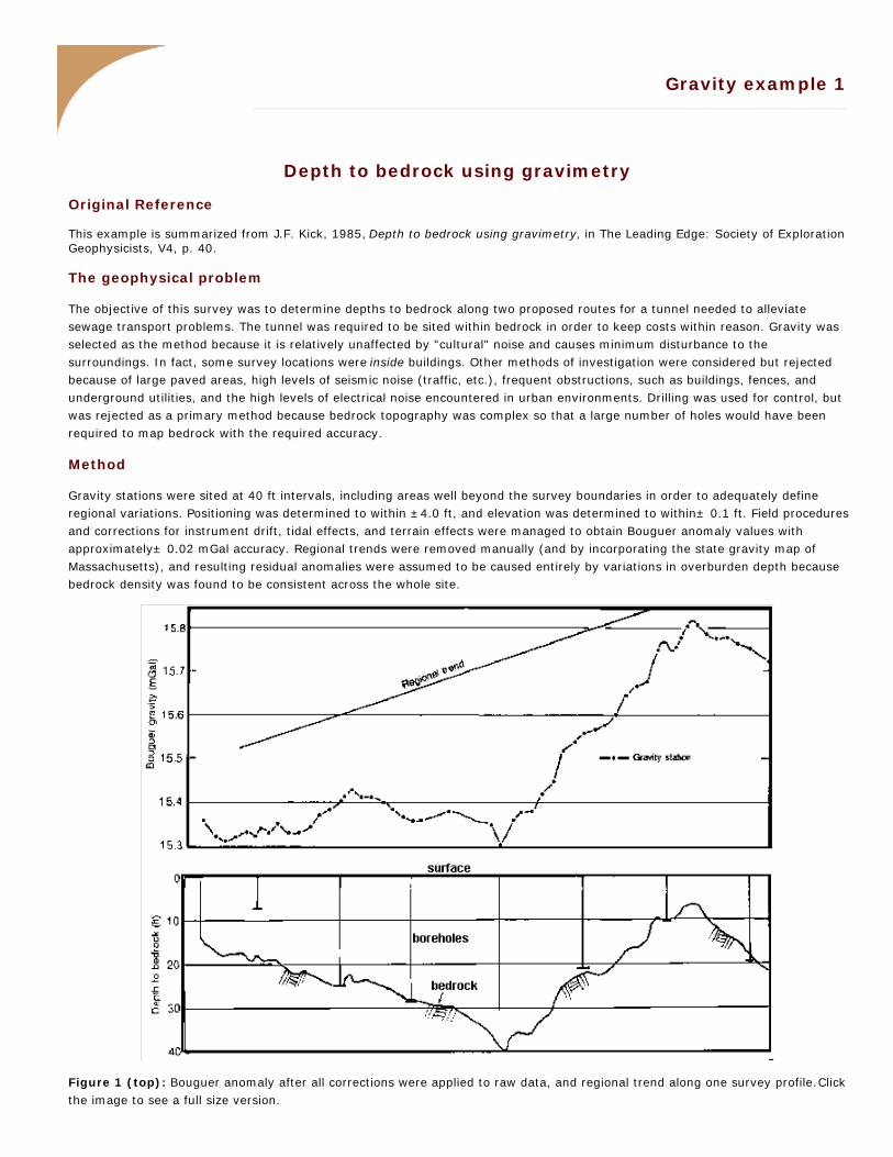
Gravity stations were sited at 40 ft intervals, including areas well beyond the survey boundaries in order to adequately defineregional variations. Positioning was determined to within ±4.0 ft, and elevation was determined to within± 0.1 ft. Field proceduresand corrections for instrument drift, tidal effects, and terrain effects were managed to obtain Bouguer anomaly values withapproximately± 0.02 mGal accuracy. Regional trends were removed manually (and by incorporating the state gravity map ofMassachusetts), and resulting residual anomalies were assumed to be caused entirely by variations in overburden depth becausebedrock density was found to be consistent across the whole site.

Figure 1 (top): Bouguer anomaly after all corrections were applied to raw data, and regional trend along one survey profile. Click the image to see a full size version.

Figure 2 (bottom): Depth to bedrock interpreted from the gravity profile in Figure 1. Boreholes with depth do bedrock areshown as bars at the bottom of holes that reached bedrock. Click the image to see a full size version.

Discussion of the survey

Results shown in the figure are from one of several line profiles. Borehole control is shown, and except for one point, correlationwith bedrock horizons is very good. Depth to bedrock was estimated from gravity by using the same formula as the Bouguercorrection. In other words, instead of using more complicated modeling procedures, the anomaly due to an infinte slab with thedensity of soil was used at each location. In this case, errors caused by this approximation were not significant to the outcome,which was to estimate maximum thickness of overburden. Finally, it was noted that surveys such as this can be cost effective ifskilled operators are involved, but success depends on careful attention to details at each step in the design, acquisition,processing, and interpretation of data.

F. Jones, UBC Earth and Ocean Sciences, 01/27/2007 15:44:32

Gravity example 2

Regional trend removal for gravity anomaly detection

Original Reference

This example is summarized from C. Ferris, 1987, Gravity anomaly resolution at the Garber field, Geophysics, 52, #11, 1570-1579.

The geophysical task

The Garber oil field in north-central Oklahoma was discovered in 1916, and has been one of the largest oil fields in the state. Agravity survey started in 1939 was terminated before completion because no anomaly could be seen with the station spacing of805 m. The author returned to collect gravity data at 201 m spacing in 1950 in order to ascertain whether more careful workcould detect the anomaly expected from the formations known to be present. Figure 1a is the resulting Bouguer anomaly map,with the profile discussed below shown as A-A'.

. .

Figure 1a. Bouguer gravity map of the area of interest. Contour interval is 1 mGal. Figure 1b. Residual gravity anomaly after removing third degree best fit polynomial. The gray zone is the producing area of this

oil field.

Method

Three methods were employed to resolve the the local anomaly from the regional anomaly.

First, a third degree polynomial surface was fitted to the Bouguer anomaly map; then the resulting trend was subtractedfrom the Bouguer anomaly map. The result is shown in Figure 1b, with the oil-producing structure overlaid as a gray zone.Good correspondence between the residual anomaly and the geological structure of interest is evident.The second trend removal technique involved calculating a vertical gradient map from the Bouguer anomaly map. Resultswere similarly successful at delineating the structure.The third method involved harmonic analysis of data along the profile. Please refer to the original paper for details.

Discussion

The figure below shows the Bouguer anomaly, the polynomial regional trend, the vertical gradient, the residual after subtractingthe trend from the Bouguer anomaly, and the forward modeled response to structures associated with the oil field. Several pointsare worth noting:

It is not surprising that the original gravity survey with spacial interval of 800 m failed to identify the target. Clearly, 200 mspacing was much more appropriate.The anomaly associated with interesting structures is easy to miss if the regional trend is not properly removed.Trend removal is implicit when gradient filtering is applied. Vertical gradient filtering is shown, but horizontal gradientswould also likely identify the structure.Significant fault zones are identified by high lateral gradients in both the residual and the vertical gradient profiles.The 2D model used to calculate an expected response (using the commonly applied method of Telwani) was wellunderstood at the time of the test. There are undoubtedly other structures that could produce similar gravitational responseat the surface.

Top: Four profiles (A-A' in Figure 1) showing (top to bottom) the Bouguer gravity anomaly, the third degree polynomial, thevertical gradient, and the residual (Bouguer anomaly minus regional). The modeled response is also shown with the residualprofile. Bottom: The model used to generate the modeled profile in the top panel. Densities and geometries are quite well known from oilwell drilling that has taken place since the Garber field was discovered in 1916.

F. Jones, UBC Earth and Ocean Sciences, 01/27/2007 14:59:48

Gravity example 3

Gravity case history summary: An engineering application

This is a point-form summary of Microgravimetry for Engineering Applications, by A.A.Arzi, Geophysical prospecting 23, 1975, p408.

The geotechnical problem was to look for voids in otherwise uniform bed rock under shallow overburden. The reason was that anuclear power plant was to be built at the site, and stable foundations (not on top of voids) had to be ensured.

What follows is simply a summary of the paper. The capitalized headings, and any figures, are those used in the paper.

INTRODUCTION

Review of previous applications in the literature.

GEOLOGICAL BACKGROUND

Clayey till overburden 3 - 6 m thickSoil-bedrock interface has relief of only 1 mBedrock is horizontally layered sandy dolomite with anhydrite and gypsum with shale seams (from boreholes to 100 m).Ground water within 2 m of surface.Densities of soil and bedrock obtained from samples and lab analysis (2.0 g/cc and 2.43 g/cc respectively).

GEOPHYSICAL BACKGROUND

On this site, causes of local Bouguer gravity anomalies could be:lateral variations in bedrock or soil density,1.undulations of soil-bedrock interface,2.rock defects, i.e. solution cavities filled with rock debris, water or air.3.

Number 3 is of interest and is limited by effects of 1 and 2, plus the limitations of the survey and instrument.Anomalies of interest are "small," partly because large ones (with "wavelengths" of the order of survey dimensions, orsmall gradients) would be found by one of the few drill holes.Models show expected anomalies for various infinite cylinders (Fig. 1 in the paper).

CASE STUDIES

Verification of bedrock soundness

(This section is not reviewed here.)

Delineation of cavernous zones

Problem

A circular area (140 m diam.) was to be used for a water tower and foundations around the perimeter.Solution defects within 3 m of soil-bedrock interface were found (boring and photogeology) in the NE corner.Geophysical goal was to help determine foundation method, and foundation's exact position; i.e. to look for anomalies to delineate extent of defective zone, and to direct boring and remediation.

Survey Procedure

To ascertain "noise" level due to normal bedrock, one line done over a pit (1.6 m diameter by 1.4 m deep) on stripped bedrock.Sensitivity demonstrated by this field experiment is shown in Figure 2 of the paper. (This is a good idea, but not often donein normal engineering geophysical surveys).Instrument readings to about 3 microGal.Locations were surveyed with accuracy of 0.3 m and relative elevations of the instrument were considered good to 0.003 m(about 1 microGal of free-air error).Average ground elevation within 1 m noted to 0.03 m (about 3 microGal of Bouguer error).Then free air corrections were made using gravimeter elevations, and Bouguer corrections were made using ground elevations. The difference was significant.Drift curve shown in Figure 5 of the paper.Final errors were estimated at 4-6 microGal.Requirement was broad sampling, so spacing determined by time-frame.Soil thickness removed based on soil probes on a 30 m grid (method of Hammer, Geophysics 28, p369).Operations required a wind shield, but a 50-t bulldozer working 20 m away was not a problem.Isogal map without terrain correction produced immediately after surveying is shown below.

Results

Contour plot shows a mild NW trend, and trough around perimeter, both likely due to uncorrected terrain effect.Sharp lows in NE were repeated for verification and do not correlate specifically with topography.Small "linear" low crosses W to S.Modeling shows that defects in 3 m thick soil cover would have to be > 25%lower in density, unlikely due to history of this consolidated "stockpile"material.Drilling confirmed gravity. Extensive voids up to 1 m thick within 4.5 m of soil-bedrock interface, tapering out to the SW.Tower location shifted SW, and grouting done under foundations.Final total of >200 holes including grouting.Some repeat readings showed that most grouting migrated NE, and eastern anomaly was eliminated.Uniformly distributed defects can produce a hard to see "anomaly" that maylook like a regional trend. Drilling helps identify this effect.Excess mass may estimate grouting required, as well as verify results.

GENERAL DISCUSSION

Differences with respect to large scale gravity: i) scaling down of grids, ii)higher precision tolerances, iii) special physical environments, iv) stricttiming and economic considerations (as for all engineering work), v) demandfor conclusive answers to specific questions.Lenticular cavities < 1m thick filled with water and loose debris are visible by gravity up to 9 m above. Such thin cavities,which may include "spongework" in adjacent rock are hard to find with simple rate-of-advance drilling, but can producegravity anomalies that are greater than just the void.Necessary precision is easier to attain on a construction site than elsewhere, with little extra cost.More sites is more cost effective than more readings at each site.Each reading is of importance, and the usual spatial aliasing rules, etc. are less significant than getting anomalies to drill.Note that where other physical parameters (usually electrical) do not vary very much; density might, and gravity,therefore, may be an option in spite of the popularity of more recent methods.However, for useful results, geology, topography, etc. must be simple (as here), and conditions optimum (personnel,instruments, the site, etc.).When a method is applied close to its resolution limits, there is less room for problems and errors.

F. Jones, UBC Earth and Ocean Sciences, 01/27/2007 15:53:14