1

Gravity modelling D 5.6

2

Gravity modelling D 5.6

Version 1.0

Responsible authors: Eva Schill, Natalia Cornejo

(KIT)

Mexican partners: Marco Perez, Jonathan Carrillo-

Lopez (CICESE)

Responsible SP leader: Gylfi Páll Hersir (ÍSOR)

Responsible WP leader: Gylfi Páll Hersir (ÍSOR)

Work package 5

16.04.2019

Website: http://www.gemex-h2020.eu

The GEMex project is supported by the

European Union’s Horizon 2020

programme for Research and Innovation

under grant agreement No 727550

3

Table of Contents1

List of figures 4

List of tables 5

Executive summary 6

1 Introduction 7

1.1 Introduction to the Deliverable 5.6 7

1.2 Gravity data in reservoir exploration and engineering 7 1.2.1 Modelling of the geological subsurface structures 7 1.2.2 Determination of reservoir parameters 8 1.2.3 Monitoring of reservoir processes 9

1.3 Geological setting 9

1.4 Regional gravity data 13

2 Data acquisition and processing 15

2.1 Data acquisition 15

2.2 Data quality 16 2.2.1 Acoculco 16 2.2.2 Los Humeros 17

2.3 Processing 19

2.4 Bouguer anomalies 20

3 Residual anomalies of Los Humeros and Acoculco 24

3.1 Acoculco 24

3.2 Los Humeros 25

4 Butterworth filtering 26

4.1 Acoculco 26

4.2 Los Humeros 29

5 Inversion of gravity data from Los Humeros and Acoculco 32

5.1 Acoculco 34

5.2 Los Humeros 35

6 Conclusion 36

1 The content of this report reflects only the authors’ view. The Innovation and Networks Executive Agency

(INEA) is not responsible for any use that may be made of the information it contains.

4

List of figures

Figure 1: E-W profile through the Los Humeros volcanic complex including the four main lithostratigraphic groups

(Carrasco-Nuñez et al., 2017a). From the bottom to the top: Green (Pre-volcanic basement): limestones rocks (K),

shale and limestone rocks (J). Pink (Pre-caldera): andesities and dacitic lavas (Tpa), andesitic and dacitic lavas

(Tm). Orange (Caldera): Xaltipan Ignimbrite (QigX), Zaragoza Ignimbrite (QigZ),pre-caldera rhyolites (Qr2).

Yellow (Post- caldera): undefined pyroclastic deposits (Qp), olivine basaltic lavas (Qb1), rhyodacites and

andesites (Qrd-a), andesites basaltic andesites (Qa-ab). H-20, H-25 and H20: CEF wells. ..................................... 10

Figure 2: Volcano-tectonic faults’ architecture at Los Humeros from morpho-structural analysis: preliminary results

(Piccardi, 2018). ....................................................................................................................................................... 12

Figure 3: Simplified structural setting of the Acoculco area (Deliverable 4.1). ............................................................... 13

Figure 4: Regional Bouguer anomalies for a material density of 2670 kg cm-3 including the study areas of a) Acoculco

and b) Los Humeros (source: Comisión Nacional de Hidrocarburos, http://www.gob.mx/cnh). Large white square:

extension of the caldera areas; small white square: extension of the geothermal field and newly acquired field

survey. ...................................................................................................................................................................... 14

Figure 5: Location of the gravity stations (white dots) of the 11-12/17 and 04-05/18 surveys at a) Acoculco and b) Los

Humeros. The colour bar shows the topography in meters (WGS 84 / UTM zone 14N). ....................................... 16

Figure 6: Number of gravity measurements in the 0.03 mGal-standard deviation windows of the Acoculco survey. ..... 17

Figure 7: Number of GPS measurements in the 0.05 m standard deviation windows of vertical position of the Acoculco

survey. ...................................................................................................................................................................... 17

Figure 8: Number of gravity measurements in the 0.02 mGal-standard deviation windows of a) the 11-12/17 and b) the

04/18 surveys in Los Humeros. ................................................................................................................................ 18

Figure 9: Number of GPS measurements in the 0.01 mm standard deviation windows of vertical position of a) the 11-

12/17 and b) the 04/18 surveys in Los Humeros. ..................................................................................................... 19

Figure 10: Digital elevation model (DEM) of the Los Humeros area with a resolution of 1 m (source: Centro Mexicano

de Innovación en Energía Geotérmica (CeMIEGeo) ............................................................................................... 20

Figure 11: Topographic height versus gravity for Bouguer densities of 2100, 2400 and 2670 kg m-3 after Nettleton

(1939). ...................................................................................................................................................................... 21

Figure 12: Bouguer anomaly of the Acoculco a) geothermal and b) caldera area compared to the fault zones according

to Deliverable 4.1. .................................................................................................................................................... 22

Figure 13: Bouguer anomaly of the Los Humeros a) geothermal and b) caldera area compared to the fault zones

according to Carrasco Nuñez et al., 2017a. .............................................................................................................. 23

Figure 14: Residual anomaly of the Acoculco a) geothermal and b) caldera area compared to the fault zones according

to Deliverable 4.1. .................................................................................................................................................... 24

Figure 15: Residual anomaly of the Los Humeros a) geothermal and b) caldera area compared to the fault zones

according to Carrasco Nuñez et al., 2017a. .............................................................................................................. 25

Figure 16: Residual anomaly of the Acoculco caldera area obtained by high-pass filtering using a) 3 km, b) 6 km, c)

10 km, and d) 20 km wavelength compared to the fault zones according to Deliverable 4.1. ................................. 27

5

Figure 17: Residual anomaly of the Acoculco caldera geothermal area obtained by high-pass filtering using a 20 km

wavelength compared to the fault zones according to Deliverable 4.1. The green stars reveal the locations of the

geothermal wells in Acoculco. ................................................................................................................................. 28

Figure 18: Residual anomaly of the Acoculco caldera area obtained by band-pass filtering using a) 6-10 km, b) 6-20 km,

and c) 6-30 km, d) 10-30 km, and e) 20-30 km wavelength compared to the fault zones according to Deliverable

4.1. ........................................................................................................................................................................... 29

Figure 19: Residual anomaly of the Los Humeros caldera area obtained by high-pass filtering using a) 3 km, b) 6 km, c)

10 km, and d) 20 km wavelength compared to the fault zones according to Carrasco Nuñez et al., 2017a............. 31

Figure 20: Residual anomaly of the Los Humeros caldera area obtained by band-pass filtering using a) 6-10 km, b) 6-

20 km, and c) 6-30 km, d) 10-30 km, and e) 20-30 km wavelength compared to the fault zones according to

Carrasco Nuñez et al., 2017a. .................................................................................................................................. 32

Figure 21: Top and 3-D views of the inversion grids of Acoculco (a, b) and Los Humeros (c, d), respectively. The

colored dots represent the gravity stations. .............................................................................................................. 33

Figure 22: Density distribution obtained from 3-D inversion of gravity data of the Acoculco area at a) 2500 m a.s.l., b)

1000 m a.s.l., c) 1000 m b.s.l and d) 3000 m b.s.l. Densities are provided as Δρ (103 kg m-3) with respect to the

Bouguer density of 2670 kg m-3. Black lines indicate the faults at the surface. ....................................................... 34

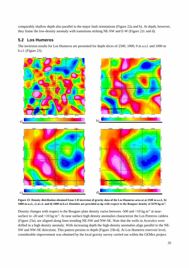
Figure 23: Density distribution obtained from 3-D inversion of gravity data of the Los Humeros area at a) 2500 m a.s.l.,

b) 1000 m a.s.l., c) at s.l. and d) 1000 m b.s.l. Densities are provided as Δρ with respect to the Bouguer density of

2670 kg m-3. ............................................................................................................................................................. 35

Figure 24: Density distribution obtained from 3-D inversion of gravity data of the Los Humeros area along the 31 km

long, NE-SW striking profile. Densities are provided as Δρ with respect to the Bouguer density of 2670 kg m-3. . 36

List of tables

Table 1.1: Bulk density of outcrops samples taken in Los Humeros. () = represents the number of analysed plugs. ...... 11

Table 1.2: Bulk density of samples from the Los Humeros reservoir (source: Comisión Federal de Electricidad, CFE). ()

= represents the number of analysed plugs. ............................................................................................................. 11

Table 4.1: Frequency ranges of the high- and band-pass filters applied to the Bouguer anomalies of Los Humeros and

Acoculco. ................................................................................................................................................................. 26

6

Executive summary

The present report includes a comprehensive presentation of the gravity data from Los Humeros and

Acoculco. It includes processing of the data newly acquired within the GEMex project during two field

surveys in 2017 and 2018 in cooperation with CICESE. In Acoculco, a total of 84 gravity stations were

acquired in 05/18 in an about 5 x 3 km rectangular grid oriented NE-SW and NW-SE with a typical station

distance of 400 m to each other. In Los Humeros, a total of 344 gravity stations were measured in two

different surveys. Between 11/17 and 12/17, 263 stations were measured along ten E-W profiles of 5.5 km

length with typical inter-station and inter-profile distances of 200 m and 500 m, respectively. In 04/18, the

survey was completed by a NE-SW oriented and 31 km long profile across the 11-12/17 study area. This

profile includes 81 gravity station with an inter-station distance of about 375 m. In total, 341 stations were

used for further evaluation in Los Humeros field.

Form Bouguer anomalies residual anomalies were calculated and analysed in a pseudo-tomography by

Buttterworth filtering. The residual anomalies of both areas were related to their structural inventory.

Indication for caldera structures as well as faults were identified. To obtain unconstrained information on the

influence of the caldera and fault structures, the planned forward modelling was replaced by inverse

modelling.

Both, residual anomalies and inversion results reveal a high fault control on the gravity and thus the density

distribution. The alignment of the majority of the anomalies follows NE-SW and NW-SE trending fault

orientations. This observation provides new insights into the structural setting of the two areas and may

contribute to the improvement of the geological models.

At reservoir level, areas of high-density anomalies in Acoculco coincide with areas of relatively low-quality

geothermal condition. A significant high-density anomaly is observed down to sea level in the area, where

the two geothermal wells were drilled. At Los Humeros, the N-S trending secondary faults in the northern

part of the geothermal field also coincide with relatively high-density anomalies, whereas the NE-SW to E-

W trending secondary faults are characterized by low-density.

7

1 Introduction

1.1 Introduction to the Deliverable 5.6

The present report "Gravity Modelling" represents the deliverable D5.6 of the H2020 funded project

"Cooperation in Geothermal energy research Europe-Mexico for development of Enhanced Geothermal

Systems and Superhot Geothermal Systems, GEMex". It refers to the work carried out in Work Package 5 "

Detection of deep structures", Task 5.3 "Evaluation of other geophysical data" and Task 5.4 "Integration of

methods and inversion constraints".

Deliverable D5.6 aims at forecasting potential new reservoir zones by analysing the subsurface density

distribution for lateral variation related to fault zones. The data presented here focus on the reservoir zone.

The report introduces

1) the potential applications of gravimetric methods in geothermal reservoir exploration,

2) the geological constraints that have been taken into account for the design of the measurements and

the interpretation of the gravimetric data, and

3) the data, anomalies and inversion obtained from earlier regional gravimetric data that were

investigated in cooperation with colleagues from the Ensenada Center for Scientific Research and

Higher Education, CICESE, in Mexico. The results of this cooperation were submitted for

publication in Geophysics in 2018 (Carrillo et al., subm.).

The report describes the data acquisition of new, high-resolution gravimetric data in Los Humeros and

Acoculco in cooperation with CICESE, their processing (chapter 2), anomalies (chapter 3), filtering (chapter

4) and inversion (chapter 5). It puts the newly acquired data in context compared with the regional gravity

data.

1.2 Gravity data in reservoir exploration and engineering

In reservoir exploration and engineering relative gravity data are acquired using relative gravimeters to

obtain the gravity difference at a point of observation and a reference point. In the following, we discuss the

fields of application of gravity data with regard to reservoir exploration and engineering. Against the

background of the results obtained by filtering the residual anomalies in chapter 4, major attention of the

gravity modelling is given to the link between joints, fractures and faults with low gravity anomalies such as

described in section 1.2.2 of the chapter.

1.2.1 Modelling of the geological subsurface structures

Reservoir exploration in a first step focuses on the assessment of the structural 3-D geological setting of the

reservoir zone. Typically, this is accomplished by a multi-method approach integrated into a 3-D geological

model. It takes into account geological surface data (2-D), geophysical data (1- to 3-D) of and borehole data

(1-D) in the subsurface. In most cases, geological data are sparse and there is no information between

geological maps, cross sections or boreholes (Calcagno et al., 2008).

In the case of geothermal exploration in crystalline rock, a detailed structural 3-D geological model of the

reservoir is important in order to understand the complex fault and pathway system. Apart from

understanding permeability anisotropy in joint systems, it is also crucial for the reactivation potential during

reservoir engineering (Faulds et al., 2010).

8

Forward modelling of gravity data, i.e. the establishment of a density-depth relation, may be used to infer

units of different density in the subsurface that principally relate to different geologic units. Forward

modelling involves a starting model for the source body of an anomaly that is constructed on geological and

geophysical constraints. The model’s anomaly is calculated and compared with the observed anomaly, and

the model parameter are adjusted iteratively in order to improve the fit between the two anomalies (Blakley,

1996). However, intrinsic for all potential field methods is the infinite number of possible solutions. Thus,

best advantage of potential field data may be taken using integrative approaches.

In this context, Guillen et al. (2008) have developed a 3D probabilistic geological modelling approach from

field data and geological knowledge, using gravity and magnetic data inversion to validate the models. The

method, called “total litho-inversion”, allows identify the most probable or the best model testing all the

possibilities in a range of different geometries. It starts with a priori model, where the geological maps

provide a representation of the distribution of the main geological units that has to be extrapolated at depth

surface. At the same time, the geological units constitute the elementary cells of a model and are define by

independent parameters such as the nature of the lithology, the topology of the geological units, the shape of

the units and intrinsic properties (density, susceptibility, magnetization, porosity, thermal conductivity, and

radioactivity). First, the 3-D geometrical model has to be constrained by the information provided by the

geological maps. Then, considering the intrinsic properties mentioned before, those parameters can be

assigned to each geological unit and their effects in the 3-D geometric models can be calculated and

compared with the corresponding measured potential fields. In this way, direct and inverse modelling can

provide and infinite number of model that satisfied the gravity and magnetic fields and their tensors. For the

forward modelling, the geological models have to be constructed assembling homogeneous voxels with

adjustable density contrast, and analytical expressions are used to calculate their effects in the potential

fields. In the case of the inversion, the lithology is the primary model parameter to be introduced into the

discretized 3-D geological model. During the inversion, the lithology of the surface voxels is keeping fixed,

and the lithology associated to the subsurface is free to vary. This variation to the initial model try to

reproduce the measured potential fields, so the change in the misfit between the measured and computed

potential fields is determined and examined in a probabilistic framework to accept or not the modification in

the model.

1.2.2 Determination of reservoir parameters

Besides on mineralogical composition, density of rocks and thus its gravimetric response at the surface

depends on porosity. The determination of porosity in geothermal systems by means of gravity

measurements has been applied, for example at the Geysers field, where according the phase of the fluid,

porosity changes in the order of 0.5 to 1.6% have been attributed to density changes of 40 to 60 kg m-3 for

reservoir zones of an extension of several kilometres (Denlinger et al., 1981). In this case, density changes

were related to porosity through measurements of the interconnected porosity on samples. In Alpine low-

temperature geothermal systems, negative gravity anomalies have been linked to faults along which

geothermal fluid rises naturally (Guglielmetti et al., 2013). At regional scale, spatial coincidence of low

density and thermal anomalies in the Upper Rhine Graben of central Europe has been attributed to fracture

porosity occurring in the fault zones that host the geothermal reservoirs of the area (Baillieux et al., 2013).

Gravity in combination with 3-D geological modelling has proven to be an appropriate tool for visualization

of fracture porosity in the granitic basement (Baillieux et al., 2014). Quantification of fracture porosity was

achieved using 3-D seismic data as structural subsurface model (Altwegg et al., 2015). The 3-D seismic

subsurface model is discretized into vertical prisms and for each unit the effect on gravity is calculated using

the algorithm of Blakely (1996). The effect of the structures that are irrelevant for the determination of

fracture porosity were subtracted from the observed residual anomaly by sequential stripping. This approach

9

was applied successfully to the Sankt Gallen geothermal project (Switzerland, Altwegg et al., 2015) that

targeted a fault zone that affects Mesozoic sediments at a depth of about 4500 m. The spatial extension of

these sediments, a major fault zone and indication for graben structures in the crystalline basement were

observed in the 3-D seismic model. Both the graben and the fault zone coincided with negative gravity

anomalies. After stripping gravity effects of geothermally irrelevant geological units from the residual

anomaly, local faults were assumed to account for remaining anomalies. Synthetic case study on the effect of

density variation and considerable gas content in the well supported possible fracture porosity between about

4 and 8 %.

1.2.3 Monitoring of reservoir processes

Gravity allows for monitoring changes in the mass balance in the subsurface. It has been successfully applied

to conventional geothermal fields. For example, between 1980 and 1991 in the production zone of the Bulalo

geothermal reservoir gravity decreases by > 250 mGal in response to fluid withdrawals. Mass discharge and

recharges predicted by reservoir simulation modelling generally matches changes inferred from the observed

gravity data (San Andres and Pedersen, 1993). Deep liquid pressure draw down in the 1960s in the Wairakei

geothermal field resulted in the formation of a steam zone with subsequent saturation changes in the steam

zone, liquid temperature decline, and ground-water level changes. Gravity changes (corrected for

subsidence) of up to -1±0.3 mGal a 1 km2 area of the production field and smaller decreases extending over a

50 km2 surrounding area were the consequence (Allis and Hunt, 1986). First the measurements near

Rittershoffen (France) show a signal above the noise level which correlates in time with a production test

(Hinderer et al. 2015).

1.3 Geological setting

The Los Humeros and Acoculco Volcanic Complexes are located in the eastern part of the Trans Mexican

Volcanic Belt, an active continental volcanic arc formed by the subduction of the Cocos and Rivera plates

beneath the North American plate along the Middle American trench (Ferrari et al., 2012). Their

emplacement is associated Pleistocene-Holocene volcano tectonic structures (e.g. Norini et al., 2015).

The complex evolution of the Los Humeros Complex involves alternated episodes of effusive and explosive

eruptions in a basaltic-andesite-rhyolite system (e.g. Yáñez and García, 1982), which are attributed to the

formation of the Los Humeros caldera with the inner Los Potreros caldera (Carrasco-Núñez et al., 2017). For

a complete discussion on Los Humeros geology and related aspects, the reader is referred to Carrasco-Núñez

et al. (2017).

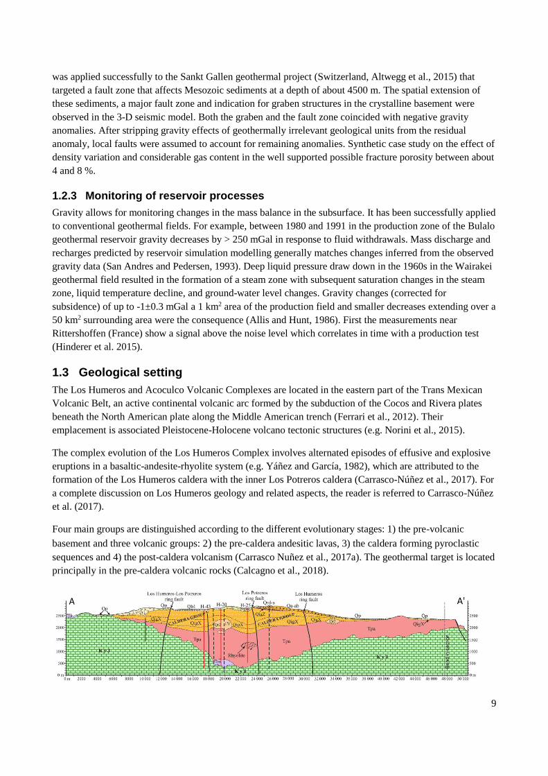
Four main groups are distinguished according to the different evolutionary stages: 1) the pre-volcanic

basement and three volcanic groups: 2) the pre-caldera andesitic lavas, 3) the caldera forming pyroclastic

sequences and 4) the post-caldera volcanism (Carrasco Nuñez et al., 2017a). The geothermal target is located

principally in the pre-caldera volcanic rocks (Calcagno et al., 2018).

10

Figure 1: E-W profile through the Los Humeros volcanic complex including the four main lithostratigraphic groups

(Carrasco-Nuñez et al., 2017a). From the bottom to the top: Green (Pre-volcanic basement): limestones rocks (K), shale and

limestone rocks (J). Pink (Pre-caldera): andesities and dacitic lavas (Tpa), andesitic and dacitic lavas (Tm). Orange

(Caldera): Xaltipan Ignimbrite (QigX), Zaragoza Ignimbrite (QigZ),pre-caldera rhyolites (Qr2). Yellow (Post- caldera):

undefined pyroclastic deposits (Qp), olivine basaltic lavas (Qb1), rhyodacites and andesites (Qrd-a), andesites basaltic

andesites (Qa-ab). H-20, H-25 and H20: CFE wells.

In Acoculco, Avellán et al. (2018) and Sosa-Ceballos et al. (2018) distinguish eight units: partly covered by

Holocene alluvial deposits, six units are related to the late Miocene to late Pleistocene volcanic activity, and

one represents the Jurassic-Cretaceous calcareous basement.

In order to characterize the reservoirs in Acoculco and Los Humeros according to their rock properties in

Deliverable 6.1 a number of > 250 rocks samples were studied. Among those 770 density measurements

were carried out. Table 1.1 shows the results for the density values of outcrops samples taken in Los

Humeros divided into basement and intrusive rocks, pre-caldera volcanism, caldera volcanism and post-

caldera volcanism, and the Table 1.2 shows the density values of reservoir samples provided by Comisión

Federal de Electricidad (CFE).

Groups Formation Bulk density ρB [kg m-3]

Post-caldera Volcanism Basalt lava (altered) 2280 ± 180 (28)

Ash fall deposits 1220 ± 130 (6)

Caldera volcanism Inner caldera ignimbrite 1550 ± 120 (20)

Xaltipán ignimbrite 1570 ± 200 (30)

Xaltipán ignimbrite (altered) 2420 ± 10 (9)

Pre-caldera volcanism Andesite total 2510 ± 170 (166)

Teziutlán andesite 2650 ± 50 (82)

Teziutlán andesite (porous) 2290 ± 140 (37)

Cuyoaco andesite/dacite 2390 ± 70 (23)

Alseseca andesite 2580 ± 50 (20)

Toba ignimbrite 2420 ± 30 (12)

Basement and intrusive rocks Quartz veines 2540 ± 70 (13)

Skarn 3360 ± 490 (77)

Marble 2690 ± 120 (56)

Chert 2590 ± 10 (2)

Shales 2660 ± 10 (6)

11

Limestone K 2670 ± 90 (146)

Limestone J 2600 ± 20 (11)

Calcarenite J 2070 ± 80 (6)

Granite/Granodiorite 2640 ± 150 (26)

Table 1.1: Bulk density of outcrops samples taken in Los Humeros. ( ) = represents the number of analysed plugs.

Formation Bulk density ρB [kg m-3]

Andesite 2410 ± 150 (85)

Ignimbrite 2310 ± 140 (14)

Tuff 2020 ± 270 (7)

Basalt 2320 ± 180 (20)

Marble 2680 ± 40 (3)

Table 1.2: Bulk density of samples from the Los Humeros reservoir (source: Comisión Federal de Electricidad, CFE).

( ) = represents the number of analysed plugs.

Recalling that major attention of the gravity modelling is given to the link between fracture zones and faults

with low gravity anomalies, in the following, this section focuses on the structural setting.

The Los Humeros Volcanic Complex is characterized by the coexistence of two volcano-tectonic structural

systems: (1) the caldera faults of the Los Humeros and Los Potreros calderas and (2) the NNW–SSE, N–S,

NE–SW and E–W-striking faults in the Los Potreros Caldera (Norini et al., 2015). Morpho-structural

analysis reveal NW-SE, SE-NW and E-W striking structures outside the caldera (Deliverable 4.1). Piccardi

(2018) distinguishes, NE-SW structures, which exhibit the major control on the intrusion of magma at Los

Humeros and Las Minas area, appear to be oldest. This set of faults does not show pronounced evidence of

recent activity. The Perote fault seems to have been reactivated by the volcanic ring-structures.

The E-W to ENE-WSW oriented structures appear to control the emplacement of the magma at depth. They

represent a conduit for flow at least since about 3’000 yrs ago (Carrasco-Núñez et al., 2017). The NW-SE

oriented structures have relationships both, with similarly oriented compressional structures observed in the

far-field of the caldera and with the normal faults which affect the volcanic complex in and outside of the

caldera area. The approximately N-S oriented structures, controlling the main caldera rims of Los Humeros

and Los Potreros, appear to be the most recent one, being limited in extension within the volcanic edifice and

representing the main conduits for the fluids circulating in the Los Humeros geothermal field. Major fault

zones that are considered in the evaluation of the gravity data are displayed in Figure 2.

12

Figure 2: Volcano-tectonic faults’ architecture at Los Humeros from morpho-structural analysis: preliminary results

(Piccardi, 2018).

The Acoculco caldera shows the Atotonilco scarp in the north, the Manzanito fault to the southwest and the

venting sites on the eastern and southern part, defining an asymmetric caldera extending over 18 x 16 km

(Avellán et al., 2018). Faults with similar orientation were detected in the Acoculco area (Sosa-Cabellos et

al., 2018; Deliverable 4.1). The two major families of faults with maximum length of 15 km and tens of

meters of thickness are NW-SE and SW-NE oriented. The NW-SE faults are the most prominent and appear

to intersect the SW-NE oriented fault systems. The NW-SE faults generally dip at high angle (between 70°

and 80°) to the SW. Minor E-W structures framed in the caldera evolution are also reported. Major fault

zones that are considered in the evaluation of the gravity data are displayed in Figure 3.

13

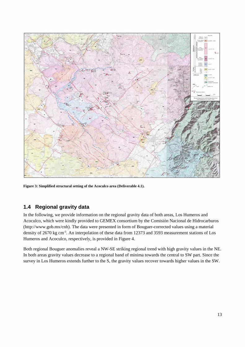
Figure 3: Simplified structural setting of the Acoculco area (Deliverable 4.1).

1.4 Regional gravity data

In the following, we provide information on the regional gravity data of both areas, Los Humeros and

Acoculco, which were kindly provided to GEMEX consortium by the Comisión Nacional de Hidrocarburos

(http://www.gob.mx/cnh). The data were presented in form of Bouguer-corrected values using a material

density of 2670 kg cm-3. An interpolation of these data from 12373 and 3593 measurement stations of Los

Humeros and Acoculco, respectively, is provided in Figure 4.

Both regional Bouguer anomalies reveal a NW-SE striking regional trend with high gravity values in the NE.

In both areas gravity values decrease to a regional band of minima towards the central to SW part. Since the

survey in Los Humeros extends further to the S, the gravity values recover towards higher values in the SW.

14

a)

b)

Figure 4: Regional Bouguer anomalies for a material density of 2670 kg cm-3 including the study areas of a) Acoculco and b)

Los Humeros (source: Comisión Nacional de Hidrocarburos, http://www.gob.mx/cnh). Large white square: extension of the

caldera areas; small white square: extension of the geothermal field and newly acquired field survey.

15

2 Data acquisition and processing

In the following, we describe the acquisition and processing of the data that have been acquired during the

GEMex project at the study areas. For further evaluation and modelling these newly acquired data are

merged with a part of the regional data in order link them to the regional structures. Merging has been

carried out by determining the offset between the gravity of selected stations within a radius of 50 m.

2.1 Data acquisition

Gravity data have been acquired in two field campaigns in 11-12/17 and 04-05/18 in the two study areas

(Figure 4) using a CG-5 Autograv Gravity Meter (Scintrex Ltd.) with an accuracy of 0.001 mGal. This

gravimeter measures continuously by averaging a series of 6 Hz samples. At each gravity station, three

measurements of 120 s (in the survey 11-12/17) and of 240 s (in the survey 04-05/18) were acquired. The

coordinates of each gravity station were determined by differential GPS using two Trimble 5700 receivers

and two Trimble antennas (TRM39105 and TRM41249).

1) Acoculco (Figure 5a)

In Acoculco, a total of 84 gravity stations were acquired in 05/18 in an about 5 x 3 km rectangular grid

oriented NE-SW and NW-SE with a typical station distance of 400 m to each other.

2) Los Humeros (Figure 5b)

In Los Humeros, a total of 344 gravity stations were measured in two different surveys. Between 11/17 and

12/17, 263 stations were measured along ten E-W profiles of 5.5 km length with typical inter-station and

inter-profile distances of 200 m and 500 m, respectively. Of these, two measurements were rejected due to

unreliable GPS records. In 04/18, the survey was completed by a NE-SW oriented and 31 km long profile

across the 11-12/17 study area. This profile includes 81 gravity station with an inter-station distance of about

375 m, of which one measurement was rejected due unreliable GPS record. This profile runs parallel to the

most prominent negative gravity anomaly of the study area and shall be used to investigate local density

variations within this prominent structure. In total, 341 stations were used for further evaluation in Los

Humeros field.

16

a)

b)

Figure 5: Location of the gravity stations (white dots) of the 11-12/17 and 04-05/18 surveys at a) Acoculco and b) Los

Humeros. The colour bar shows the topography in meters (WGS 84 / UTM zone 14N).

2.2 Data quality

The data quality bases on the measurement accuracy of the differential GPS (vertical: 5 mm) and the

gravimeter (0.001 mGal) and the standard deviation of the gravity and GPS measurements. During the

surveys, gravity measurements were repeated three times. The measurement with lowest standard deviation

was selected for further investigation.

2.2.1 Acoculco

The standard deviation of the raw gravity measurements of 240 s at each station ranges from 0.004 to

0.197 mGal (Figure 6). The quality of gravity measurements is comparably high with about 95.2% of the data

17

revealing a standard deviation ≤ 0.03 mGal. Setting a threshold of 0.05 mGal of maximum standard deviation,

98.8% of the data (83 stations) were used for further evaluation.

Figure 6: Number of gravity measurements in the 0.03 mGal-standard deviation windows of the Acoculco survey.

The standard deviation of the GPS measurements range from 0.0015 to 1.18 m (Figure 7). The quality of the

differential GPS measurements is comparably high with about 92.8% of the data revealing a standard deviation

< 0.05 m. Setting a threshold of 0.2 m of maximum standard deviation, 97.6% of the data (82 stations) were

used for further evaluation. Taking into account the quality of the gravity and GPS measurements, a total of

79 stations were later processed in Acoculco.

Figure 7: Number of GPS measurements in the 0.05 m standard deviation windows of vertical position of the Acoculco

survey.

2.2.2 Los Humeros

For the 11-12/17 campaign with a single measurement duration of 120 s, the distribution of standard deviations

of the three raw gravity measurements at each station is shown in

Figure 8a. The values range between 0.008 and 0.119 mGal. Compared to Acoculco, the quality of gravity

with about 63.2% of the data revealing a standard deviation ≤ 0.03 mGal measurements is lower. Therefore,

in the 04/18 campaign the measurement duration was increased to 240 s, resulting however in comparable

range of standard deviations, with 62.5% of the data revealing a standard deviation ≤ 0.03 mGal (

Figure 8b). In Los Humeros, a threshold of 0.05 mGal of maximum standard deviation results in 93.5% of the

data (319 stations) being used for further evaluation.

18

a)

b)

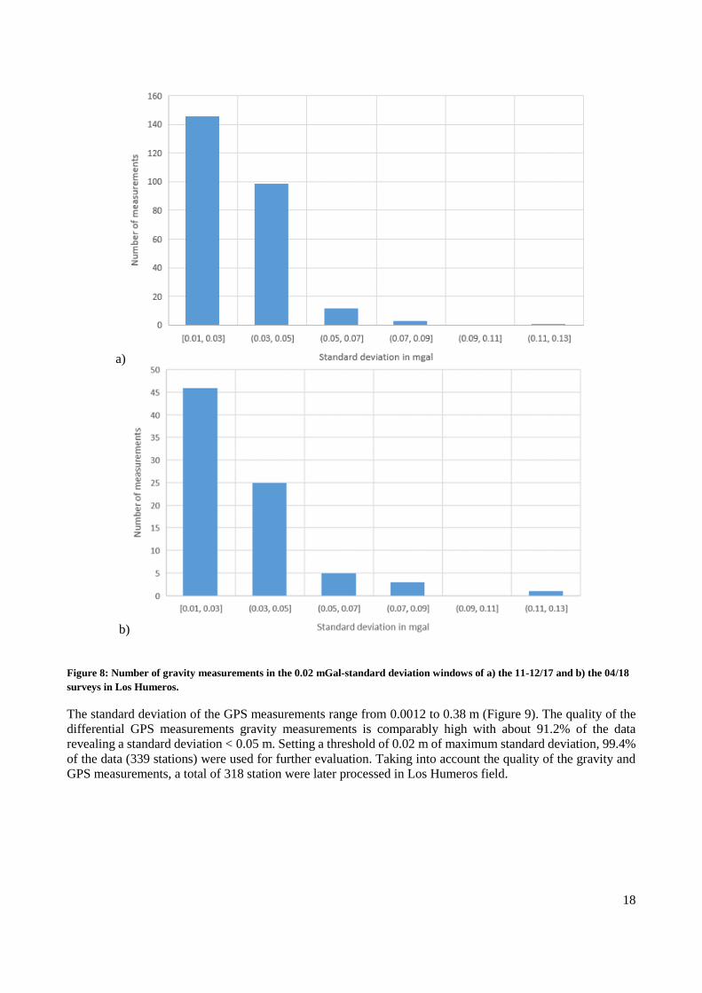
Figure 8: Number of gravity measurements in the 0.02 mGal-standard deviation windows of a) the 11-12/17 and b) the 04/18

surveys in Los Humeros.

The standard deviation of the GPS measurements range from 0.0012 to 0.38 m (Figure 9). The quality of the

differential GPS measurements gravity measurements is comparably high with about 91.2% of the data

revealing a standard deviation < 0.05 m. Setting a threshold of 0.02 m of maximum standard deviation, 99.4%

of the data (339 stations) were used for further evaluation. Taking into account the quality of the gravity and

GPS measurements, a total of 318 station were later processed in Los Humeros field.

19

a)

b)

Figure 9: Number of GPS measurements in the 0.01 mm standard deviation windows of vertical position of a) the 11-12/17

and b) the 04/18 surveys in Los Humeros.

2.3 Processing

Processing of the data has been carried out using GravProcess (Cattin et al., 2015). The procedure includes

the following steps:

1) integration of gravity data, station location, and gravity line connection input files,

2) gravity data reduction applying solid-Earth tide and instrumental drift corrections,

3) automatic network adjustment and alignment to the base stations, and

4) free air and simple Bouguer reduction.

Simple Bouguer reduction is calculated from the plateau formulation for 10 different densities ρ between

1300 and 3300 kg m-3 and the gravitational constant G = 6.67·10-11 N m2 kg-2. Due to the large amount of

data, for the calculation of the complete Bouguer reduction, the software was changed (see section 2.4).

20

2.4 Bouguer anomalies

Complete Bouguer reduction is obtained out using Oasis montaj™ Gravity and terrain Correction extension

(Geosoft). This software bases on algorithms formulated in Kane (1962) and Nagy (1966) and incorporates

advancements in grid-mesh interpolation, zoning and desampling techniques.

The terrain correction is carried out to a distance of 167 km from each gravity station. For the Acoculco

gravity data, a digital elevation model (DEM) with a resolution of 15 m from the Instituto Nacional de

Estadística y Geografía (INEGI) is used, whereas for Los Humeros, an additional dataset with 1 m resolution

of the Centro Mexicano de Innovación en Energía Geotérmica (CeMIEGeo, Figure 10) was available in the

near-field. The vertical uncertainty of the CeMIEGeo data set is reported to be 1-2 m.

Figure 10: Digital elevation model (DEM) of the Los Humeros area with a resolution of 1 m (source: Centro Mexicano de

Innovación en Energía Geotérmica (CeMIEGeo)

As the gravitational effect of a prism decreases with the square of the distance, we reduced the resolution of

the DEM with increasing distance from the gravity station as follows:

1) for Acoculco: (a) from the station, 0 m, to 100 m using the DEM with a cell size of 15 m; (b) from

100 m to 10 km a reduced cell size of 100 m; (c) to 100 km a reduced cell size of 500 m; and to

167 km a reduced cell size of 5000 m, and

2) for Los Humeros: (a) from the station, 0 m, to 10 m using the DEM with a cell size of 1 m (for points

outside of the high resolution DEM: from the station, 0 m, to 150 m using the DEM with a cell size

21

of 15 m); (b) from 10 m to 20 km a reduced cell size of 50 m; (c) to 100 km a reduced cell size of

500 m; and to 167 km a reduced cell size of 5000 m.

Given the standard deviation threshold of the GPS measurements, the uncertainty introduced by the terrain

correction is estimated to be <0.06 mGal. The uncertainty introduced by the DEM is approximately

0.6 mGal, summing up with the standard deviation threshold of the gravity measurements of 0.05 mGal to a

mean uncertainty of about 0.7 mGal.

Comparable to the simple Bouguer anomaly, also the complete Bouguer anomaly is tested for three different

densities to infer the optimum density of the Bouguer plate. In the following, we present a cross-correlation

between the topographic height and gravity along the NE-SW, 31 km long profile of Los Humeros for

Bouguer plate densities 2100, 2400 and 2670 kg m-3 (Figure 11). These values are representative for the

majority of the rocks occurring in the area (Table 1.1). Generally, the analysis of topography versus Bouguer

anomalies reveals low correlation coefficients along the profile for the densities 2100, 2400 and 2670 kg m-3.

However, the overall trend of low gravity with low elevation seems to disappear at lower Bouguer plate

densities.

Figure 11: Topographic height versus gravity for Bouguer densities of 2100, 2400 and 2670 kg m-3 after Nettleton (1939).

In the following, we will present the resulting complete Bouguer anomalies for Acoculco and Los Humeros

that combine the newly acquired and processed gravity data of GEMex with a selection of the regional data

from the Comisión Nacional de Hidrocarburos. While to local data have been acquired in high resolution on

the geothermal fields, the latter are required for connecting the geothermal field to relevant dominant

structures within and outside of the calderas. Note that the Bouguer reduction of the regional data was

carried out for a density of 2670 kg m-3. In order to merge the two data sets, the optimum Bouguer density

obtained in Figure 11 is not respected from this point on.

Both Bouguer anomalies show clear trends of decreasing gravity from NE to SW (Figure 12 and Figure 13).

This regional trend of the Bouguer anomaly is well known in the area (e.g. Urrutia-Fucugauchi and Flores-

22

Ruiz, 1996). It represents the crustal thickness increase from the Gulf of Mexico margin toward the

continental interior and is irrelevant for geothermal reservoir exploration.

a)

b)

Figure 12: Bouguer anomaly of the Acoculco a) geothermal and b) caldera area compared to the fault zones according to

Deliverable 4.1.

23

a)

b)

Figure 13: Bouguer anomaly of the Los Humeros a) geothermal and b) caldera area compared to the fault zones according to

Carrasco Nuñez et al., 2017a.

24

3 Residual anomalies of Los Humeros and Acoculco

The regional trend observed in Figure 12 and Figure 13 has been fitted using a Gaussian filter with a

standard deviation of 0.03648 mGal across the data from the stations shown in Figure 4. This has been

verified with a polynomial regression of 2nd order on the gravity values of the stations (Carrillo et al., subm.).

The calculated regional anomaly was subtracted from the Bouguer anomaly, resulting in the residual

anomaly presented in Figure 14 and Figure 15.

3.1 Acoculco

a)

b)

Figure 14: Residual anomaly of the Acoculco a) geothermal and b) caldera area compared to the fault zones according to

Deliverable 4.1.

25

3.2 Los Humeros

a)

b)

Figure 15: Residual anomaly of the Los Humeros a) geothermal and b) caldera area compared to the fault zones according to

Carrasco Nuñez et al., 2017a.

26

4 Butterworth filtering

Butterworth filter (Butterworth, 1930) is characterized and controlled mainly by two parameters,

the cut-off frequency or wavelength and

the filter order.

The advantage of the Butterworth filter is that we can easily use different wavelength to

1) delineate and characterize different negative anomalies at depth, and

2) to choose an adequate residual anomaly which provides the comparable gravity response with

the conceptual model.

Depth and size of the origin of the anomalies are indicated among others by the wavelength of the filter.

With increasing wavelength, we are able to visualize increasing larger or deeper structures until approaching

the Bouguer anomaly. Moreover, the filter order parameter can be also changed to delineate very small

variations, for instance, in the case of low density contrasts. With increasing filter order the horizontal

density contrast is emphasized.

In both areas, high- and band-pass Butterworth filters were applied to the Bouguer anomalies. The respective

frequency ranges are provided in Table 4.1.

Butterworth filters Wave length (km)

High-pass 3, 6, 10, 20

Band-pass 6-30, 10-30, 20-30

6-40, 10-40, 20-40, 30-40

3-6, 3-10, 3-20

6-10, 6-20, 6-30

Table 4.1: Frequency ranges of the high- and band-pass filters applied to the Bouguer anomalies of Los Humeros and

Acoculco.

In the following, we will present the results for the caldera areas of Acoculco and Los Humeros. Generally

high-pass filters with increasing wavelength reveal anomalies that are either at the near-surface and of

increasingly lateral extent or located at increasingly vertical depth.

4.1 Acoculco

High-pass filters with increasing wavelength from 3 to 20 km applied to the Bouguer anomaly of Acoculco

are presented in Figure 19. The dynamic of gravity changes from about 2 to 11 mGal at 3 and 20 km

wavelength, respectively. Assuming a minimum accuracy of about 0.7 mGal (see section 2.4), small and

randomly distributed anomalies observed in the 3 km high-pass filter (Figure 19a) are to a large part within

the uncertainty of the measurements. The dynamic increases in the 6 km high-pass filter to values above the

presumed detection limit of 0.7 mGal (Figure 19b). At a high-pass filter wavelength of 10 km a comparably

rough gravity topography develops, which becomes smoother with increasing wavelength (Figure 19c and

d). The latter is comparable to the residual anomaly obtained from Gaussian filtering (Figure 14Figure 15).

27

a)

b)

c)

d)

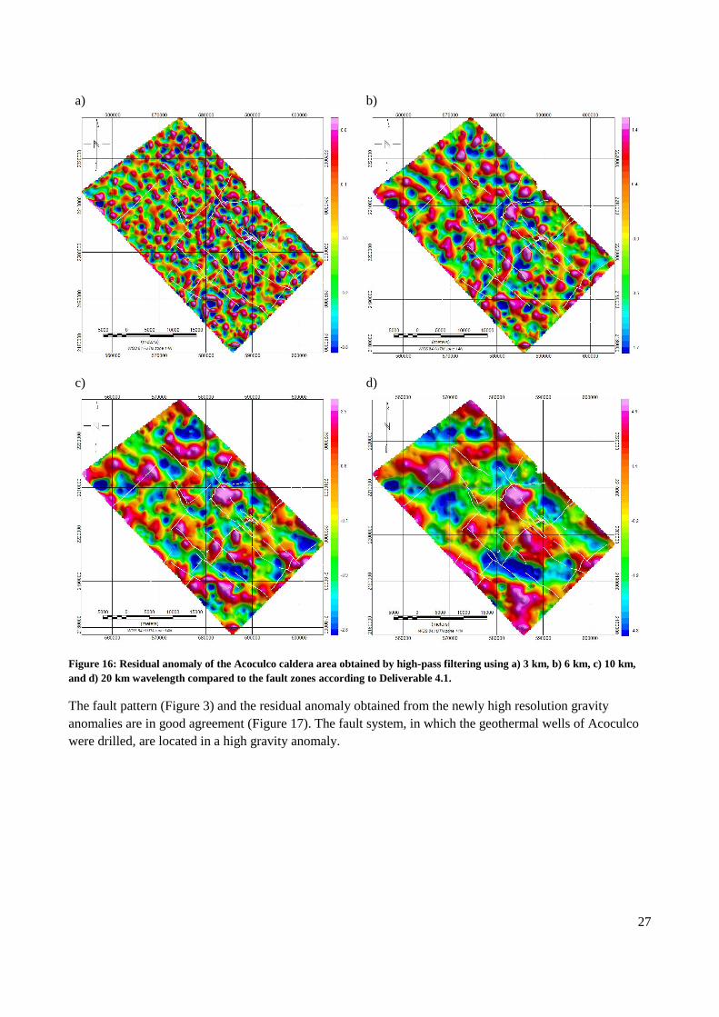
Figure 16: Residual anomaly of the Acoculco caldera area obtained by high-pass filtering using a) 3 km, b) 6 km, c) 10 km,

and d) 20 km wavelength compared to the fault zones according to Deliverable 4.1.

The fault pattern (Figure 3) and the residual anomaly obtained from the newly high resolution gravity

anomalies are in good agreement (Figure 17). The fault system, in which the geothermal wells of Acoculco

were drilled, are located in a high gravity anomaly.

28

Figure 17: Residual anomaly of the Acoculco caldera geothermal area obtained by high-pass filtering using a 20 km

wavelength compared to the fault zones according to Deliverable 4.1. The green stars reveal the locations of the geothermal

wells in Acoculco.

a)

b)

29

c)

d)

e)

Figure 18: Residual anomaly of the Acoculco caldera area obtained by band-pass filtering using a) 6-10 km, b) 6-20 km, and

c) 6-30 km, d) 10-30 km, and e) 20-30 km wavelength compared to the fault zones according to Deliverable 4.1.

Assuming that the wavelength represents depth, band-pass filters indicate that vertical extension of the

observed structural elements. In Figure 18, we present band-pass filters with a minimum wavelength of 6 km

and increasingly longer wavelength from 10 to 30 km (Figure 18a-c), as well as wavelengths of 10 to 30 km

and 20-30 km applied to the Bouguer anomaly of Acoculco. The residual anomaly after band-pass filtering

with a wavelength of 6-10 km in Figure 18a, reveals a smoothed pattern of anomalies compared to the 20 km

high-pass filtered anomalies in Figure 16d. This pattern persist with decreasing detail up to high-pass filter

wavelengths of 6-20 km, 6-30 km, and 10-30 km (Figure 18b-d). It dissolves in the band-pass filtered

residual anomaly with a wavelength of 20-30 km representing relatively large depth (Figure 18e).

4.2 Los Humeros

High-pass filters with increasing wavelength from 3 to 20 km applied to the Bouguer anomaly of Los

Humeros are presented in Figure 19. The dynamic of gravity changes from about 2 to 13 mGal at 3 and

30

20 km wavelength, respectively. Assuming a minimum accuracy of about 0.7 mGal (see section 2.4), small

and randomly distributed anomalies observed in the 3 km high-pass filter (Figure 19a) are to a large part

within the uncertainty of the measurements. A pattern of connected low and high gravity anomalies that are

above the detection limit of 0.7 mGal start appearing in the 6 km high-pass filter (Figure 19b) and

consolidate in the 10 and 20 km high-pass filter (Figure 19c and d). The latter is consistent with the residual

anomaly obtained from Gaussian filtering (Figure 15).

While the anomalies obtained from the 10 km filter reveal a ring-shaped high gravity anomaly that coincides

with the Los Potreros and Los Humeros calderas (Figure 19c), the geothermal field appears as a low gravity

anomaly. Note that this anomaly is the target of the new 11-12/17 gravity survey. This structural setting

dissolves with increasing wavelength of the high-pass filter. At a wavelength of 20 km, both high and low

gravity anomalies align along the structural directions discussed in section 1.3. The major low gravity

anomaly strikes in NE-SW direction across the entire caldera and beyond. It is, however, crosscut by a NW-

SE striking high gravity anomaly that coincides with the rim of the geothermal field.

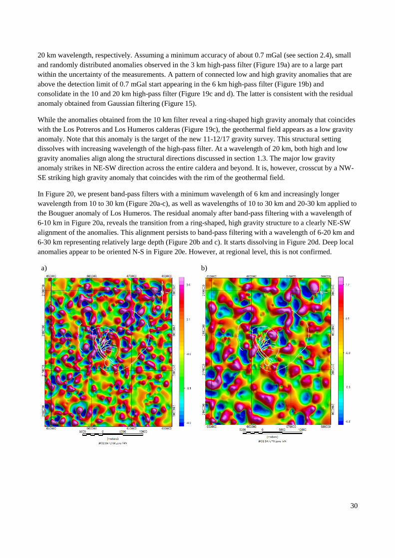
In Figure 20, we present band-pass filters with a minimum wavelength of 6 km and increasingly longer

wavelength from 10 to 30 km (Figure 20a-c), as well as wavelengths of 10 to 30 km and 20-30 km applied to

the Bouguer anomaly of Los Humeros. The residual anomaly after band-pass filtering with a wavelength of

6-10 km in Figure 20a, reveals the transition from a ring-shaped, high gravity structure to a clearly NE-SW

alignment of the anomalies. This alignment persists to band-pass filtering with a wavelength of 6-20 km and

6-30 km representing relatively large depth (Figure 20b and c). It starts dissolving in Figure 20d. Deep local

anomalies appear to be oriented N-S in Figure 20e. However, at regional level, this is not confirmed.

a)

b)

31

c)

d)

Figure 19: Residual anomaly of the Los Humeros caldera area obtained by high-pass filtering using a) 3 km, b) 6 km, c)

10 km, and d) 20 km wavelength compared to the fault zones according to Carrasco Nuñez et al., 2017a.

a)

b)

32

c)

d)

e)

f)

Figure 20: Residual anomaly of the Los Humeros caldera area obtained by band-pass filtering using a) 6-10 km, b) 6-20 km,

and c) 6-30 km, d) 10-30 km, and e) 20-30 km wavelength compared to the fault zones according to Carrasco Nuñez et al.,

2017a.

5 Inversion of gravity data from Los Humeros and Acoculco

The Butterworth filtering reveals in both areas a structural setting that differs partly from the geological

models provided in Deliverable 3.4. In the Acoculco area, a deeper dome structure is not revealed by gravity

33

data (Figure 18). In the Los Humeros area, we observe deep linear structures tending in NW-SE and NE-SW

directions (Figure 20). For this reason, forward approaches based on the geological models of Deliverable

3.4 are not expected to provide a satisfactory model to explain the gravity data. In the following, we will

instead provide results from unconstrained gravity inversion.

The inversion was performed in VOXI Earth modelling (Oasis Montaj, Geosoft), which generates 3-D voxel

models from gravity data. The model is obtained using the inverse solution of the forward modeling equation

based on Tikhonov regularization (Tikhonov, 1977), by minimizing a total objective function composed of

the data objective function and the model objective function. The regularization of the parameters is chosen

in order to maintain a suitable data misfit. The number of iterations depends on a fix misfit of 0.05 mGal

between the observed data and the predicted data.

The 3-D inversion grids of the Acoculco and Los Humeros areas (Figure 21) extend over 15 km and 14 km

in E-W and 14.5 km and 13.2 km in N-S directions, respectively. The horizontal cell size is 300 x 300 m.

The vertical extension increases gradually from 20 m below the surface to 469 m at 3000 m b.s.l. The NE-

SW profile in Los Humeros extends over 31 km. Thus, a second inversion was carried out covering the entire

profile and extending over 30 km in E-W and 27 km in N-S directions with a horizontal mesh of

600 x 600 m and vertical extensions ranging from 50 to 465 m.

a) b)

c) d)

Figure 21: Top and 3-D views of the inversion grids of Acoculco (a, b) and Los Humeros (c, d), respectively. The colored dots

represent the gravity stations.

In the following, inversion results are presented first in horizontal sections for comparison with the results

from the filtering in section 4. In addition, we present the inversion results along the 31 km long NE-SW

34

profile. The results were obtained after 37 iterations in Los Humeros and 31 iterations in Acoculco. The

inversion of the profile converges after 25 iterations.

5.1 Acoculco

The inversion results for Acoculco are presented for depth slices of 2500 and 1000 m a.s.l. and 1000 and

3000 m b.s.l. (Figure 22).

a) b)

c) d)

Figure 22: Density distribution obtained from 3-D inversion of gravity data of the Acoculco area at a) 2500 m a.s.l., b) 1000 m

a.s.l., c) 1000 m b.s.l and d) 3000 m b.s.l. Densities are provided as Δρ (103 kg m-3) with respect to the Bouguer density of

2670 kg m-3. Black lines indicate the faults at the surface.

Density changes with respect to the Bouguer plate density varies between -400 and +10 kg m-3 at near

surface to -40 and +20 kg m-3. At near surface anomalies are aligned along lines trending NE-SW and NW-

SE. Note that the wells in Acoculco were drilled in a high-density anomaly (Figure 22a). With increasing

depth, the anomalies connect to larger structure. The low density anomalies align in NE-SW and NW-SE

direction (Figure 22b) and concentrate in a single anomaly at increasing depth (Figure 22c and d). The high-

density anomalies among those the anomaly in which the two geothermal wells were drilled, align at

35

comparably shallow depth also parallel to the major fault orientations (Figure 22a and b). At depth, however,

they frame the low-density anomaly with transitions striking NE-SW and E-W (Figure 22c and d).

5.2 Los Humeros

The inversion results for Los Humeros are presented for depth slices of 2500, 1000, 0 m a.s.l. and 1000 m

b.s.l. (Figure 23).

a) b)

c) d)

Figure 23: Density distribution obtained from 3-D inversion of gravity data of the Los Humeros area at a) 2500 m a.s.l., b)

1000 m a.s.l., c) at s.l. and d) 1000 m b.s.l. Densities are provided as Δρ with respect to the Bouguer density of 2670 kg m-3.

Density changes with respect to the Bouguer plate density varies between -500 and +10 kg m-3 at near-

surface to -20 and +10 kg m-3. At near surface high density anomalies characterize the Los Potreros caldera

(Figure 23a). are aligned along lines trending NE-SW and NW-SE. Note that the wells in Acoculco were

drilled in a high density anomaly. With increasing depth the high-density anomalies align parallel to the NE-

SW and NW-SE directions. This pattern persists to depth (Figure 23b-d). At Los Humeros reservoir level,

considerable improvement was obtained by the local gravity survey carried out within the GEMex project.

36

The inversion results reveal that the N-S trending secondary faults in the northern part of the geothermal

field also coincide with relatively high-density anomalies, whereas the NE-SW to E-W trending secondary

faults are characterized by low-density.

The results along the NE-SW profile connects the local survey to the regional density distribution. Its

inversion results are shown in Figure 24.

Figure 24: Density distribution obtained from 3-D inversion of gravity data of the Los Humeros area along the 31 km long,

NE-SW striking profile. Densities are provided as Δρ with respect to the Bouguer density of 2670 kg m-3.

6 Conclusion

With the aim of forecasting potential new reservoir zones the subsurface density distribution of Acoculco

and Los Humeros was analysed for lateral variation related to fault zones.

Both, residual anomalies and inversion results reveal a high fault control on the gravity and thus the density

distribution. The alignment of the majority of the anomalies follows NE-SW and NW-SE trending fault

orientations. At reservoir level, areas of high-density anomalies in Acoculco coincide with areas of relatively

low-quality geothermal condition. A significant high-density anomaly is observed down to sea level in the

area, where the two geothermal wells were drilled. At Los Humeros, the N-S trending secondary faults in the

northern part of the geothermal field also coincide with relatively high-density anomalies, whereas the NE-

SW to E-W trending secondary faults are characterized by low-density.

37

Assuming a link between low density zones related to faults and fractures, we recommend to compare the

gravity and density distributions to active faults with high reactivation potential.

Comparing our results to other geophysical measurements, such as magnetotellurics (Deliverable 5.2), we

would like to point out that we observed coincidence with the orientation of these observables, for instance,

the induction arrows and phase tensor orientations. We therefore, strongly recommend a joint inversion of

magnetotelluric and gravity data in Task 5.4.

38

7 References

Allis RG, Hunt TM (1986) Analysis of exploitation-induced gravity changes at Wairakei

geothermal field. Geophysics 51:1647–1660

Altwegg P., Schill E., Abdelfettah Y., Radogna P.-V., Mauri G. (2015) Toward fracture porosity

assessment by gravity forward modeling for geothermal exploration (Sankt Gallen, Switzerland).

Geothermics 57, 26–38.

Altwegg, P., Renard, P., Schill, E., Radogna, P.-V., 2015. GInGER (GravImetry forGeothermal

ExploRation): a new tool for geothermal exploration using grav-ity and 3D modelling software. In:

Proc. World Geothermal Congress 2015, Melbourne, Australia, p. 7.

Baillieux, P., Schill, E., Abdelfettah, Y., Dezayes, C., 2014. Possible natural fluid path-ways from

gravity pseudo-tomography in the geothermal fields of NorthernAlsace (Upper Rhine Graben).

Geotherm. Energy 2, http://dx.doi.org/10.1186/s40517-014-0016-y

Baillieux, P., Schill, E., Edel, J.-B., Mauri, G., 2013. Localization of temperature anoma-lies in the

Upper Rhine Graben: insights from geophysics neotectonic activity.Int. Geol. Rev. 55, 1744–1762.

Blakely, R.J., 1996. Potential Theory in Gravity and Magnetic Applications. Cambridge University

Calcagno, P., Courrioux, G., Guillen, A., Chilès, J.-P., 2008. Geological modelling from field data

and geological knowledge. Part I. Modelling method coupling 3D potential-field interpolation and

geological rules. Physics of the earth and planetary interiors.

Carrasco-Núñez, G., López-Martínez, M., Hernández, J., and Vargas, V.: Subsurface stratigraphy

and its correlation with the surficial geology at Los Humeros geothermal field, eastern Trans-

Mexican Volcanic Belt, Geothermics, 67, 1–17, https://doi.org/10.1016/j.geothermics.2017.01.001,

2017a.

Carrasco-Núñez, G., Hernández, J., De Léon, L., Dávilla, P., Norini, G., Bernal, J. P., Jicha, B.,

Jicha, B., Navarro, M., and López-Quiroz, P.: Geologic Map of Los Humeros volcanic complex and

geothermal field eastern Trans-Mexican Volcanic Belt, Terra Digitalis, 1, 1–11, 2017b.

Cattin, R., Mazzotti, S., Baratin, L.-M., 2015. GravProcess: an easy-to-use MATLABsoftware to

process campaign gravity data and evaluate the associated un-certainties. Comput. Geosci. 81, 20–

27.http://dx.doi.org/10.1016/j.cageo.2015.04.005

Denlinger, R., Isherwood, W., Kovach, R., 1981. Geodetic analysis of reservoir deple-tion at The

Geysers steam field in northern California. J. Geophys. Res. Solid Earth86, 6091–6096.

Ferrari, L., Orozco-Esquivel, T., Manea, V., Manea, M., 2012. The dynamic history of the Trans-

Mexican Volcanic Belt and the Mexico subduction zone. Tectonophysics522–523, 122–149.

Guglielmetti, L., Comina, C., Abdelfettah, Y., Schill, E., Mandrone, G., 2013. Integrationof 3D

geological modeling and gravity surveys for geothermal prospection in anAlpine region.

Tectonophysics 608, 1025–1036.

39

Guillen, A., Calcagno, P., Courrioux, G., Joly, A., Ledru, P., 2008. Geological modelling from field

data and geological knowledge, Part II. Modelling validation using gravity and magnetic data

inversion. Physics of the Earth and Planetary Interiors 171, 158–169.

Hinderer J, Calvo M, Abdelfettah Y, Hector B, Riccardi U, Ferhat G, Bernard J-D. Monitoring of a

geothermal reservoir by hybrid gravimetry; feasibility study applied to the Soultz-sous-Forêts and

Rittershofen sites in the Rhine graben. Geothermal Energy. 2015. https://doi.org/10.1186/s40517-

015-0035-3.

Norini, G. Gropelli, G., Sulpizio, R., Carrasco-Núñez, G., Dávila-Harris, P., Pellicioli, C., Zucca,

F., and De Franco, R.: Structural analysis and thermal remote sensing of the Los Humeros Volcanic

Complex: Implications for volcano structure and geothermal exploration, J. Volcanol. Geoth. Res.,

301, 221–237, 2015.

Yañez-García, C., y García-Durán, S.. 1982: Exploración de la región geotérmlca Los Humeros-

Derrumbadas, estados de Puebla y VeraCruz: México, D.F. C.F.E

40

Coordination Office, GEMex project

Helmholtz-Zentrum Potsdam

Deutsches GeoForschungsZentrum

Telegrafenberg, 14473 Potsdam

Germany