Greater Sage-Grouse in the Southeast Montana Sage-Grouse Core Area

Melissa A. Foster1, John T. Ensign2, Windy N. Davis3, and Dale C. Tribby4 1: FWP Wildlife Biologist. Phone: (406) 852-2032. Email: mfoster@mt.gov.

2: FWP Wildlife Program Manager. Phone: (406) 234-0921. Email: jensign@mt.gov. 3: Former FWP Energy Specialist & BLM Liaison. Phone: (208) 756-2271. Email: windy.davis@idfg.idaho.gov.

4: BLM Supervisory Wildlife Biologist. Phone: (406) 233-2812. Email: dtribby@blm.gov.

MONTANA FISH, WILDLIFE AND PARKS (FWP) in partnership with:

USDI BUREAU OF LAND MANAGEMENT (BLM)

i

– EXECUTIVE SUMMARY – We studied 94 greater sage-grouse hens in the Southeastern Montana Sage-Grouse

Core Area (hereafter: Core Area) to determine demographic rates, quantify seasonal movements and habitat use, and make management recommendations. Sage-grouse Core Areas support Montana's highest densities of sage-grouse, and are high priority conservation focus areas critical to the long term sustainability and management of sage-grouse. Historic lek data (pre-1980) from the Core Area are unavailable, but lek counts conducted over the past 30 years indicate the population has not exhibited a long-term downward trend. The population peaked during the mid-2000’s but declined following a West Nile virus (WNv) outbreak in 2007. Sage-grouse have persisted at sustainable levels in the Core Area because traditional landowners have maintained large expanses of intact sagebrush-steppe habitat.

Sage-grouse in southeastern Montana were exposed to extreme weather conditions throughout the study. Precipitation during spring/summer 2010 was 53% above average. Precipitation during spring/summer 2011 was 67% above average, with 8 inches rainfall during May alone, which caused widespread flooding (100-year flood events). Drought conditions occurred during summer 2012. Above-average snowfall and below-average temperatures occurred during winter 2009-10. The following winter, 2010–11, was among the most severe on record (30 year winter event). In contrast, winter 2011–12 was among the mildest on record.

Nest initiation (91%) and renest initiation (42%) rates were high. Apparent nest success varied among years (43% in 2010, 33% in 2011, and 68% in 2012). Low nest success in 2011 was driven by extreme precipitation that caused 9% of nests to fail and depressed hatch rates. Models relating vegetation characteristics to nest survival generally performed poorly, which indicates cover did not limit nest success during the study. Chick survival averaged 29%. Forb cover was higher for successful (12.2% cover) than failed (7.9% cover) broods. Forb cover and richness were related to precipitation and higher during wet years.

Apparent nest success was higher for nests in pastures with livestock concurrently present (59%) than pastures without livestock (38%), and we observed no direct negative impacts (e.g., trampling) of livestock on nesting sage-grouse. Similarly, brood success from 0–14 days post-hatch was higher for broods hatched in pastures with livestock (79%) than without (61%). The mechanism driving this is unknown; it may have resulted from behavioral avoidance of livestock by predators, or reflect predator control efforts in areas with livestock. Our results concur with research elsewhere that livestock grazing is compatible with sage-grouse conservation.

During wet years 2010 and 2011, 36% of hatches and the bulk of the early brood-rearing period occurred after June 15 (a common end date for timing restrictions on disturbing activities associated with development projects). During drought year 2012, all nests hatched by June 10 but the early brood-rearing period extended to mid-July. We recommend timing restrictions be maintained until July 15: in most years nesting would be complete, nearly all chicks would be >2 weeks old, and most broods would have reached 30 days. Extending timing restrictions to benefit young chicks may be important because most chick mortality occurs

ii

within the first 4 weeks post-hatch, and chick survival is one of the most important parameters influencing population growth for sage-grouse. However, timing restrictions are only effective for minimally invasive, short duration projects and cannot offset the impacts of long-term habitat loss, fragmentation, or degradation.

The average distance between nests and the nearest lek was 1.15 miles, which may reflect low levels of fragmentation and relatively intact sagebrush-steppe habitat in the Core Area. Fifty-nine percent of nests were within one mile of a known lek location, 84% within 2 miles, 93% within 3 miles, and 97% within 4 miles. Nest success exerts great influence on population growth rates for sage-grouse. Therefore, a one-mile buffer is inadequate to avoid significant population impacts associated with development activities. We recommend a minimum 4 mile buffer around leks for highly-intrusive practices within suitable sagebrush habitat. A 4 mile buffer may not be feasible in all cases. As with any project or planned development, consultation with an area wildlife biologist, early in the process, is critical to avoid or minimize impacts. Brood hens tended to stay close to nest sites for the first 30 days following hatch ( = 0.68 mi), thus restrictive radii placed around leks may also benefit young broods.

Annual hen survival in the Core Area during 2011–12 and 2012–13 (59–61%) was higher than survival during 2010–11 (45%), which was driven by lower late summer/fall survival (due to a suspected WNv outbreak) and lower winter survival due to severe conditions. Mortality was attributed to primarily avian (≥40%) followed by mammalian predation (≥27%). No mortalities were attributed to collision with fences or power lines, and no hunting mortalities occurred. Population Viability Analyses (PVA) indicated that Core Area sage-grouse are very likely to persist at sustainable levels. Our most realistic scenario suggested a stable population (population growth rate = -0.8% annually) and 0% probability of extinction within 30 years. Severe weather events (floods and winter) had little impact on population growth (≤ 0.4% reduction in annual population growth) because of their rarity. The future impact of WNv is of concern because few tools exist to reduce WNv outbreaks, the severity of future outbreaks is impossible to reliably predict, and PVA indicated that the Core Area sage-grouse population is not undergoing rapid recovery since the 2007 outbreak. However, PVA did indicate the population has great potential to increase if environmental conditions or management actions improve population vital rates (e.g., 17.5% increase in annual population growth rate by increasing survival and reproduction rates by 5%).

We designated 19% of the Core Area as sage-grouse winter range. Critical winter range consisted of windswept flats characterized by short shrubs ( = 7.8 in), and moderate shrub density ( = 11%). Hens used areas with taller ( = 10.2 in) sagebrush during severe winter 2010–11, and 54% percent of hens shifted their winter ranges, presumably to locate open stands of sagebrush. Other hens were apparently unable to locate suitable habitat, based on reduced survival and observations of sage-grouse roosting on a barren snowscape during the severe winter. Sage-grouse winter habitat use reflects that the Core Area is located at the eastern edge of the range of Wyoming big sagebrush, and is characterized by smaller, less dense sagebrush than elsewhere in the sage-grouse range. Sage-grouse in the study used sagebrush-steppe habitat extensively throughout their annual cycle (92% of locations), but frequently (27% of locations) used areas with sparse (1–10%) sagebrush canopy cover. Given

iii

that sagebrush characteristics may be intrinsically limited by local soil and climactic conditions, management guidelines that emphasize certain heights or densities of sagebrush may be unachievable in the Core Area. Management of sage-grouse habitat should focus on protecting the integrity of winter use and other important areas rather than sagebrush manipulation.

Movement patterns varied greatly among individual sage-grouse hens but the Core Area boundary in Montana contained nearly every location in the state, which provides evidence that the core area approach (i.e., delineating priority areas for sage-grouse conservation based on lek densities) has great potential to benefit sage-grouse. However, many hens made movements into South Dakota and Wyoming adjacent to the Core Area, and cooperation among states will be necessary to maintain this sage-grouse population. We recommend minor adjustments to the Montana Core Area and Wyoming Connectivity area to create a cohesive boundary and incorporate winter range. The South Dakota draft core area encompassed nearly all locations from radio-collared sage-grouse hens.

Traditional family-owned ranching operations, the predominant local stakeholders in the Core Area, have historically managed land in a manner that is compatible with sage-grouse conservation and are well-poised to collaborate with wildlife and range professionals to maintain and improve sage-grouse habitat. Our management recommendations are standard for sage-grouse and include the following: 1) first and foremost, maintain large expanses of intact sagebrush habitat, 2) utilize livestock grazing as a management tool (we recommend rotational grazing systems consisting of large pastures that incorporate rest during the growing season and alternate season of use), 3) implement conservation efforts on a landscape scale, including various stakeholders, 4) when projects must occur, plan to minimize the impacts, and 5) minimize the potential for WNv outbreaks where possible. We do not recommend predator control for several reasons: 1) population vital rates observed in the study were normal for sage-grouse and we expected the majority of mortalities and nest failures to be a result of predation (sage-grouse are a prey species—they do not typically die of old age, and nest predation is a fact of life that all ground nesting birds have evolved with), 2) controlling avian predators is not possible due to federal law (e.g., 1940 Bald and Golden Eagle Protection Act), 3) control of one type of predator often leads to unintended increases in other predator species, 4) predator control is expensive and only effective in the short term in small areas with intense control of all predators. In contrast, habitat management can result in economically feasible, widespread, long-term benefits for sage-grouse and livestock producers alike.

iv

– TABLE OF CONTENTS –

Executive Summary ................................................................................................................ i

List of Tables .........................................................................................................................vi

List of Figures ...................................................................................................................... viii

1. Introduction ..................................................................................................................... 1 Study Area ........................................................................................................................... 5 Capture & Radiotelemetry .................................................................................................. 6

2. Nest Success & Vegetation ................................................................................................ 9 Introduction ...................................................................................................................... 10 Methods ............................................................................................................................ 11 Nest monitoring .................................................................................................... 11 Vegetation sampling ............................................................................................. 11 Analyses ................................................................................................................ 12 Results ............................................................................................................................... 13 Nesting season dates ............................................................................................ 13 Nesting vital rates ................................................................................................. 14 Fates of failed nests .............................................................................................. 15 Nest vegetation ..................................................................................................... 16 Factors influencing nest survival ........................................................................... 18 Discussion.......................................................................................................................... 20

3. Brood Success & Vegetation ............................................................................................ 25 Introduction ...................................................................................................................... 26 Methods ............................................................................................................................ 27 Brood monitoring .................................................................................................. 27 Brood site vegetation ............................................................................................ 28 Analyses ................................................................................................................ 28 Results ............................................................................................................................... 29 Brood-rearing dates & vital rates ......................................................................... 29 Brood site vegetation ............................................................................................ 31 Factors influencing brood survival ........................................................................ 33 Discussion.......................................................................................................................... 37

4. Hen Survival……… ............................................................................................................ 42 Introduction ...................................................................................................................... 43 Methods ............................................................................................................................ 43 Results ............................................................................................................................... 44 Discussion.......................................................................................................................... 46

5. Population Viability ........................................................................................................ 48 Introduction ...................................................................................................................... 49

v

Methods ............................................................................................................................ 50 Scenarios ............................................................................................................... 51 Results ............................................................................................................................... 53 Discussion.......................................................................................................................... 53

6. Movements & Seasonal Habitat Use ............................................................................... 56 Introduction ...................................................................................................................... 57 Methods ............................................................................................................................ 57 Analyses ................................................................................................................ 58 Results ............................................................................................................................... 60 Movements ........................................................................................................... 60 Seasonal habitat use ............................................................................................. 62 Discussion.......................................................................................................................... 67

7. Winter Use & Vegetation ................................................................................................ 72 Introduction ...................................................................................................................... 73 Methods ............................................................................................................................ 73 Delineating winter use areas ................................................................................ 73 Winter vegetation ................................................................................................. 74 Results ............................................................................................................................... 75 Delineating winter use areas ................................................................................ 75 Winter vegetation ................................................................................................. 76 Discussion.......................................................................................................................... 79

8. Management Recommendations .................................................................................... 82 Maintain Large Expanses of Intact Sagebrush Habitat ..................................................... 83 Management of sagebrush habitat ...................................................................... 84

Utilize Livestock Grazing as a Management Tool ............................................................. 85 Predator Control vs. Habitat Management ...................................................................... 87 Implement Conservation Efforts on a Landscape Scale .................................................. 88 When Projects Must Occur, Plan to Minimize the Impacts .............................................. 89

Breeding, nesting, and brood-rearing ................................................................... 90 Winter Range ........................................................................................................ 91

Minimize West Nile Virus Outbreaks ................................................................................ 91

Acknowledgements ............................................................................................................. 93

Literature Cited ................................................................................................................... 94

Appendix A: Weather Conditions ........................................................................................ 105

vi

– LIST OF TABLES –

Table 2.1. Median incubation initiation date and nesting season length ................................... 14

Table 2.2. Nest and renest initiation by age class and year ........................................................ 14

Table 2.3. Apparent nest success and maximum-likelihood estimates for nest success ............ 15

Table 2.4. Vegetation characteristics at sage-grouse nest sites .................................................. 17

Table 2.5. Ranking of model strengths for daily survival rates (DSR) of sage-grouse-nests ....... 19

Table 3.1. Median and range of hatch dates ............................................................................... 30

Table 3.2. Brood success ............................................................................................................. 31

Table 3.3. Average number of chicks per successful brood at 30 days post-hatch, chick survival, and chick production per hen ...................................................................... 31

Table 3.4. Shrub characteristics at sage-grouse brood-rearing locations ................................... 32

Table 3.5. Vegetative characteristics at sage-grouse brood-rearing locations ........................... 32

Table 3.6. Forb species richness at sage-grouse brood rearing locations ................................... 33

Table 3.7. Percent occurrence of 7 common forb species at sage-grouse brood-rearing locations and average percent horizontal cover of each species ............................... 34

Table 3.8. Percent occurrence for forb species occurring at <15% of brood-rearing locations ...................................................................................................................... 35

Table 4.1. Ranking of model strengths for hen survival .............................................................. 44

Table 4.2. Seasonal and annual survival ...................................................................................... 45

Table 5.1. Parameter estimates for population viability analysis scenarios. .............................. 52

Table 5.2. Population viability analysis results ............................................................................ 53

Table 6.1. Distances between nests for hens that nested more than once during the study .... 61

Table 6.2. Distances between nest and brooding sites ............................................................... 61

Table 6.3. Average distance and total distance moved over winter ........................................... 67

Table 6.4. Fidelity to winter range for hens that were tracked more than one winter .............. 67

Table 6.5. Habitat use by season and reproductive status .......................................................... 68

Table 7.1. Sagebrush canopy cover, density, and height at sage-grouse winter locations .......... 77

Table 7.2. Slope was lower in critical versus important sage-grouse winter range ..................... 78

vii

Table 7.3. Percent of sage-grouse winter locations that were within 0.25 miles from fences, roads, trees, power lines, buildings, structures, or trees ........................................... 78

Table A.1. Spring/summer monthly precipitation totals ........................................................... 105

Table A.2. Spring/summer monthly average temperatures ...................................................... 106

Table A.3. Total monthly snowfall ............................................................................................. 107

Table A.4. Winter monthly average temperatures .................................................................... 108

viii

– LIST OF FIGURES –

Fig. 1.1. Current and historic distribution of greater sage-grouse ................................................ 2

Fig. 1.2. Sage-grouse Core Areas and study area ........................................................................... 4

Fig. 1.3. Average number of greater sage-grouse males counted per lek in Carter County, Montana, 1980-2013 ....................................................................................................... 5

Fig. 1.4. The Southeast Montana Sage-grouse Core Area contains large tracts of sagebrush-steppe habitat. ................................................................................................................. 6

Fig. 1.5. Capture locations for 94 radio collared sage-grouse hens .............................................. 7

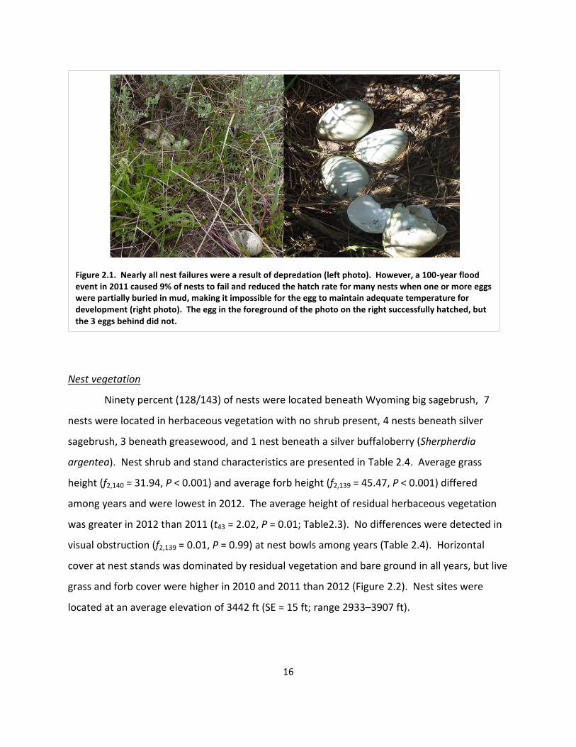
Fig. 2.1. Nearly all nest failures were a result of depredation. However, a 100-year flood event in 2011 caused 9% of nests to fail and reduced the hatch rate for many nests when one or more eggs were partially buried in mud, making it impossible for the egg to maintain adequate temperature for development ............................................ 16

Fig. 2.2. Percent horizontal cover of 5 cover classes estimated within Daubenmire (1959) frames along transects bisecting sage-grouse nests ..................................................... 18

Fig. 2.3. Results from other studies indicate that sage-grouse nests tend to be more successful when surrounding grass is taller .................................................................. 22

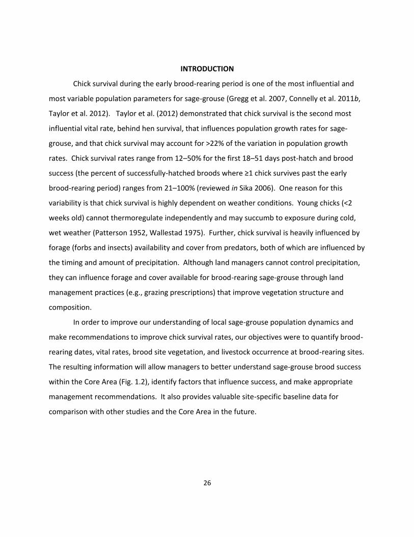
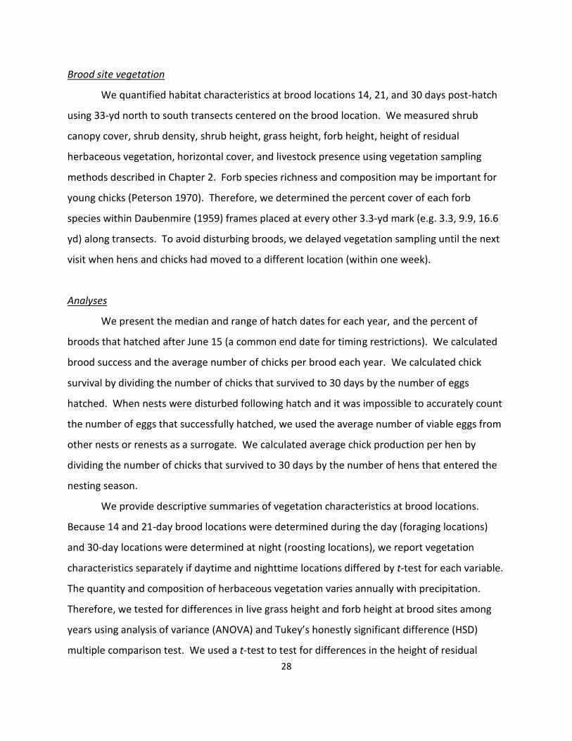
Fig. 3.1. Two week old chicks were often fully concealed underneath brood hens at night. As chicks approach 30 days old, they are too large to be fully concealed beneath the hen and can be accurately counted during nighttime brood counts ............................ 27

Fig. 3.2. Range of hatch dates, median hatch date, and early brood rearing period .................. 30

Fig. 3.3. Average percent horizontal cover for 5 habitat variables measured within Daubenmire (1959) frames along transects at sage-grouse brood-rearing locations, 2010–2012 ..................................................................................................................... 32

Fig. 3.4. Example brood rearing locations for radio collared greater sage-grouse ..................... 36

Fig. 3.5. Sweet clover dominated much of the landscape of the study area during 2011 .......... 41

Fig. 4.1. Cause-specific mortality ................................................................................................. 45

Fig. 4.2. Heavy snow cover during winter 2010–2011 reduced hiding cover and concentrated sage-grouse .................................................................................................................... 47

Fig. 5.1. Example VORTEX simulation .......................................................................................... 49

Fig. 6.1. Example movement patterns .......................................................................................... 63

Fig. 6.2. Example minimum convex polygons .............................................................................. 64

ix

Fig. 6.3. Overall dispersion of radio-collared sage-grouse during the breeding,

nesting/brood-rearing, and late summer/fall seasons. ................................................. 65

Fig. 6.4. Overall dispersion of radio-collared sage-grouse during winter.................................... 66

Fig. 7.1. Winter range polygons ................................................................................................... 76

Fig. 7.2. Examples of shrub characteristics at winter locations ................................................... 77

Fig. 7.3. Rose diagram showing aspects for winter locations. ..................................................... 78

Fig. 7.4. Winter use data was scarce for hens from the extreme northeast finger of the Core Area due to hen mortalities. It is likely that other, unidentified, winter use areas exist in Core Area south of Powderville, MT ................................................................. 80

Fig. A.1. Extraordinary precipitation during spring/summer 2010 and 2011 resulted in tremendous growth of vegetation during both years ................................................. 106

Fig. A.2. The Little Missouri River north of Albion, MT rose above 100-year flood levels during spring 2011 ....................................................................................................... 106

Fig. A.3. Below-average precipitation and above-average temperatures resulted in drought conditions during summer 2012 .................................................................................. 107

Fig. A.4. Snowfall during winter 2010-11 was nearly three times average, resulting in a vast snowscape and deep snow drifts throughout the Core Area ...................................... 108

Fig. A.5. Above-average temperatures and below-average snowfall during winter 2011-12 resulted in mild, open conditions ................................................................................ 108

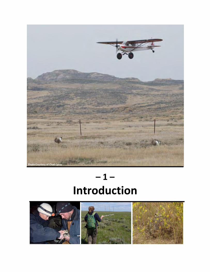
– 1 –

Introduction

Photo Courtesy of Chad Cyrus

2

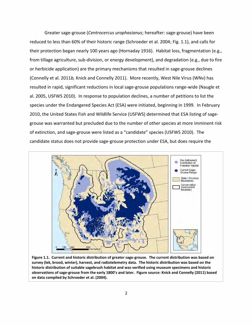
Greater sage-grouse (Centrocercus urophasianus; hereafter: sage-grouse) have been

reduced to less than 60% of their historic range (Schroeder et al. 2004; Fig. 1.1), and calls for

their protection began nearly 100 years ago (Hornaday 1916). Habitat loss, fragmentation (e.g.,

from tillage agriculture, sub-division, or energy development), and degradation (e.g., due to fire

or herbicide application) are the primary mechanisms that resulted in sage-grouse declines

(Connelly et al. 2011b, Knick and Connelly 2011). More recently, West Nile Virus (WNv) has

resulted in rapid, significant reductions in local sage-grouse populations range-wide (Naugle et

al. 2005, USFWS 2010). In response to population declines, a number of petitions to list the

species under the Endangered Species Act (ESA) were initiated, beginning in 1999. In February

2010, the United States Fish and Wildlife Service (USFWS) determined that ESA listing of sage-

grouse was warranted but precluded due to the number of other species at more imminent risk

of extinction, and sage-grouse were listed as a “candidate” species (USFWS 2010). The

candidate status does not provide sage-grouse protection under ESA, but does require the

Figure 1.1. Current and historic distribution of greater sage-grouse. The current distribution was based on survey (lek, brood, winter), harvest, and radiotelemetry data. The historic distribution was based on the historic distribution of suitable sagebrush habitat and was verified using museum specimens and historic observations of sage-grouse from the early 1800’s and later. Figure source: Knick and Connelly (2011) based on data compiled by Schroeder et al. (2004).

3

USFWS to annually review their status. This elevated status also brings about a sense of

urgency to prevent ESA listing through conservation measures such as habitat protection and

enhancement.

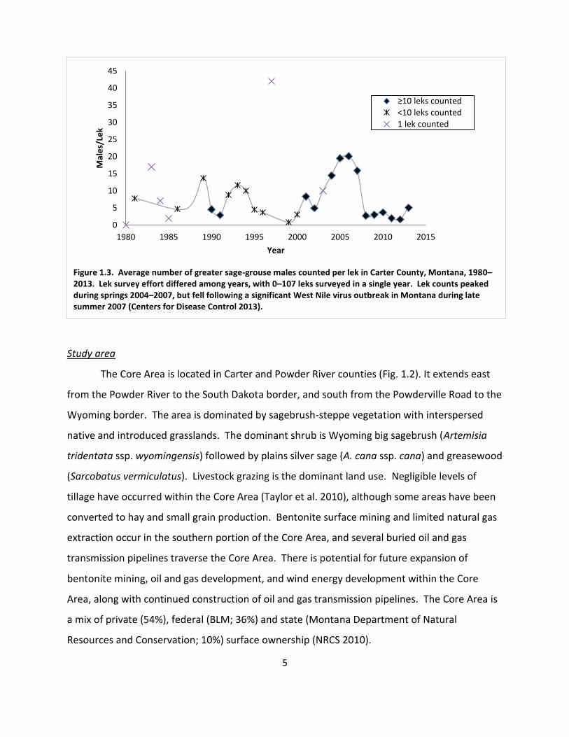
Despite population declines throughout much of the sage-grouse range, portions of

southeast Montana support stable sage-grouse populations and contain large areas of

unfragmented sagebrush-steppe habitat (Taylor et al. 2010). Montana Fish, Wildlife, and Parks

(FWP) historically monitored sage-grouse populations using hunter harvest surveys, lek counts

in a small number of geographically defined trend areas, and other opportunistic lek counts

(typically large, easily accessible leks). In response to increasing concerns over sage-grouse

populations elsewhere and lack of comprehensive lek documentation, FWP Region 7 initiated

systematic aerial survey efforts across all potential sage-grouse habitat in the region to identify

previously unknown lek locations and quantify male lek attendance. The surveys occurred over

a 10-year period and nearly doubled the number of documented lek locations in southeastern

Montana (Beyer et al. 2010). For example, of the 234 leks currently documented in Carter and

Powder River Counties, 93 (40%) were identified during systematic aerial surveys between 2006

and 2009.

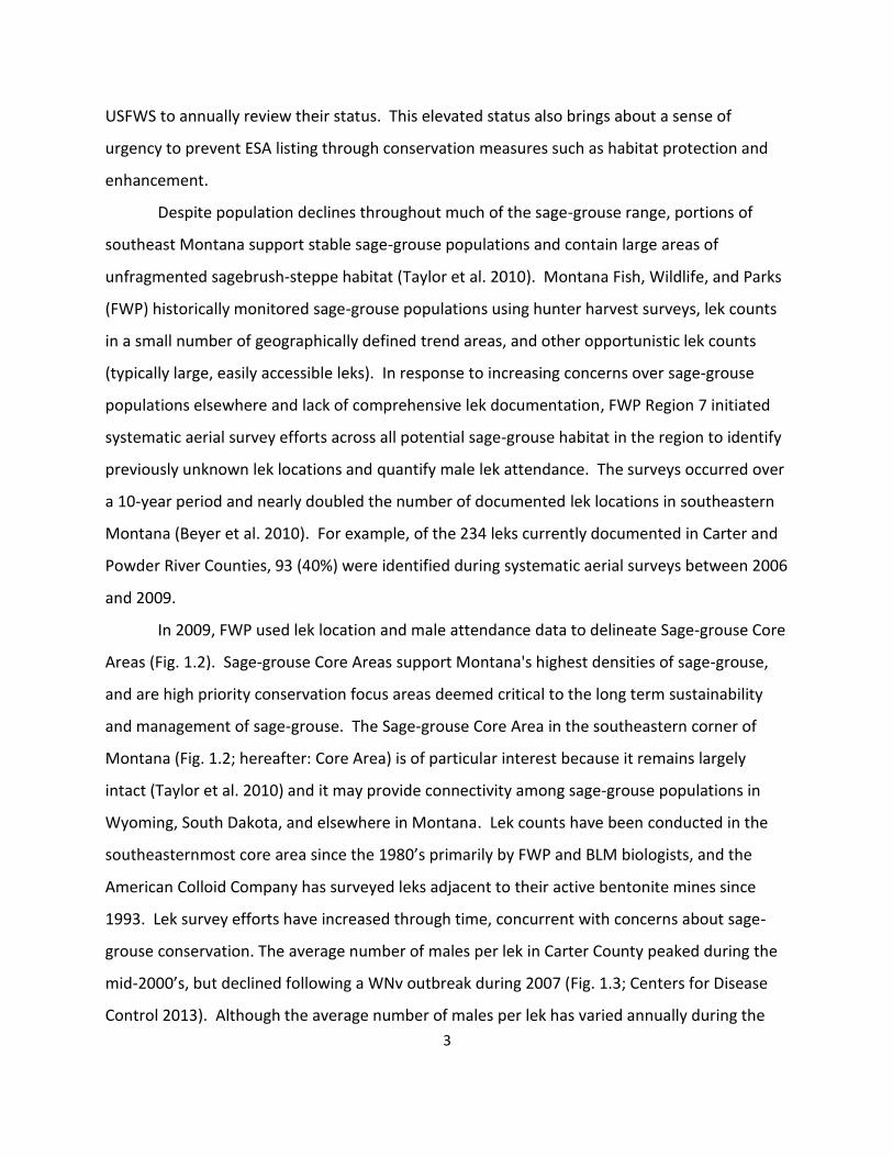
In 2009, FWP used lek location and male attendance data to delineate Sage-grouse Core

Areas (Fig. 1.2). Sage-grouse Core Areas support Montana's highest densities of sage-grouse,

and are high priority conservation focus areas deemed critical to the long term sustainability

and management of sage-grouse. The Sage-grouse Core Area in the southeastern corner of

Montana (Fig. 1.2; hereafter: Core Area) is of particular interest because it remains largely

intact (Taylor et al. 2010) and it may provide connectivity among sage-grouse populations in

Wyoming, South Dakota, and elsewhere in Montana. Lek counts have been conducted in the

southeasternmost core area since the 1980’s primarily by FWP and BLM biologists, and the

American Colloid Company has surveyed leks adjacent to their active bentonite mines since

1993. Lek survey efforts have increased through time, concurrent with concerns about sage-

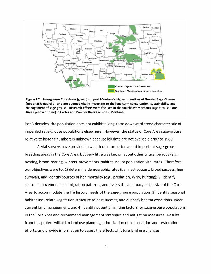
grouse conservation. The average number of males per lek in Carter County peaked during the

mid-2000’s, but declined following a WNv outbreak during 2007 (Fig. 1.3; Centers for Disease

Control 2013). Although the average number of males per lek has varied annually during the

4

Figure 1.2. Sage-grouse Core Areas (green) support Montana's highest densities of Greater Sage-Grouse (upper 25% quartile), and are deemed vitally important to the long term conservation, sustainability and management of sage-grouse. Research efforts were focused in the Southeast Montana Sage-Grouse Core Area (yellow outline) in Carter and Powder River Counties, Montana.

last 3 decades, the population does not exhibit a long-term downward trend characteristic of

imperiled sage-grouse populations elsewhere. However, the status of Core Area sage-grouse

relative to historic numbers is unknown because lek data are not available prior to 1980.

Aerial surveys have provided a wealth of information about important sage-grouse

breeding areas in the Core Area, but very little was known about other critical periods (e.g.,

nesting, brood-rearing, winter), movements, habitat use, or population vital rates. Therefore,

our objectives were to: 1) determine demographic rates (i.e., nest success, brood success, hen

survival), and identify sources of hen mortality (e.g., predation, WNv, hunting); 2) identify

seasonal movements and migration patterns, and assess the adequacy of the size of the Core

Area to accommodate the life history needs of the sage-grouse population; 3) identify seasonal

habitat use, relate vegetation structure to nest success, and quantify habitat conditions under

current land management, and 4) identify potential limiting factors for sage-grouse populations

in the Core Area and recommend management strategies and mitigation measures. Results

from this project will aid in land use planning, prioritization of conservation and restoration

efforts, and provide information to assess the effects of future land use changes.

5

Figure 1.3. Average number of greater sage-grouse males counted per lek in Carter County, Montana, 1980–2013. Lek survey effort differed among years, with 0–107 leks surveyed in a single year. Lek counts peaked during springs 2004–2007, but fell following a significant West Nile virus outbreak in Montana during late summer 2007 (Centers for Disease Control 2013).

0

5

10

15

20

25

30

35

40

45

1980 1985 1990 1995 2000 2005 2010 2015

Mal

es/

Lek

Year

≥10 leks counted <10 leks counted

1 lek counted

Study area

The Core Area is located in Carter and Powder River counties (Fig. 1.2). It extends east

from the Powder River to the South Dakota border, and south from the Powderville Road to the

Wyoming border. The area is dominated by sagebrush-steppe vegetation with interspersed

native and introduced grasslands. The dominant shrub is Wyoming big sagebrush (Artemisia

tridentata ssp. wyomingensis) followed by plains silver sage (A. cana ssp. cana) and greasewood

(Sarcobatus vermiculatus). Livestock grazing is the dominant land use. Negligible levels of

tillage have occurred within the Core Area (Taylor et al. 2010), although some areas have been

converted to hay and small grain production. Bentonite surface mining and limited natural gas

extraction occur in the southern portion of the Core Area, and several buried oil and gas

transmission pipelines traverse the Core Area. There is potential for future expansion of

bentonite mining, oil and gas development, and wind energy development within the Core

Area, along with continued construction of oil and gas transmission pipelines. The Core Area is

a mix of private (54%), federal (BLM; 36%) and state (Montana Department of Natural

Resources and Conservation; 10%) surface ownership (NRCS 2010).

6

Capture & radiotelemetry

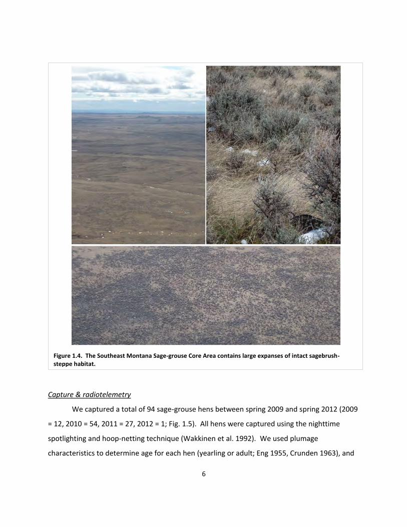
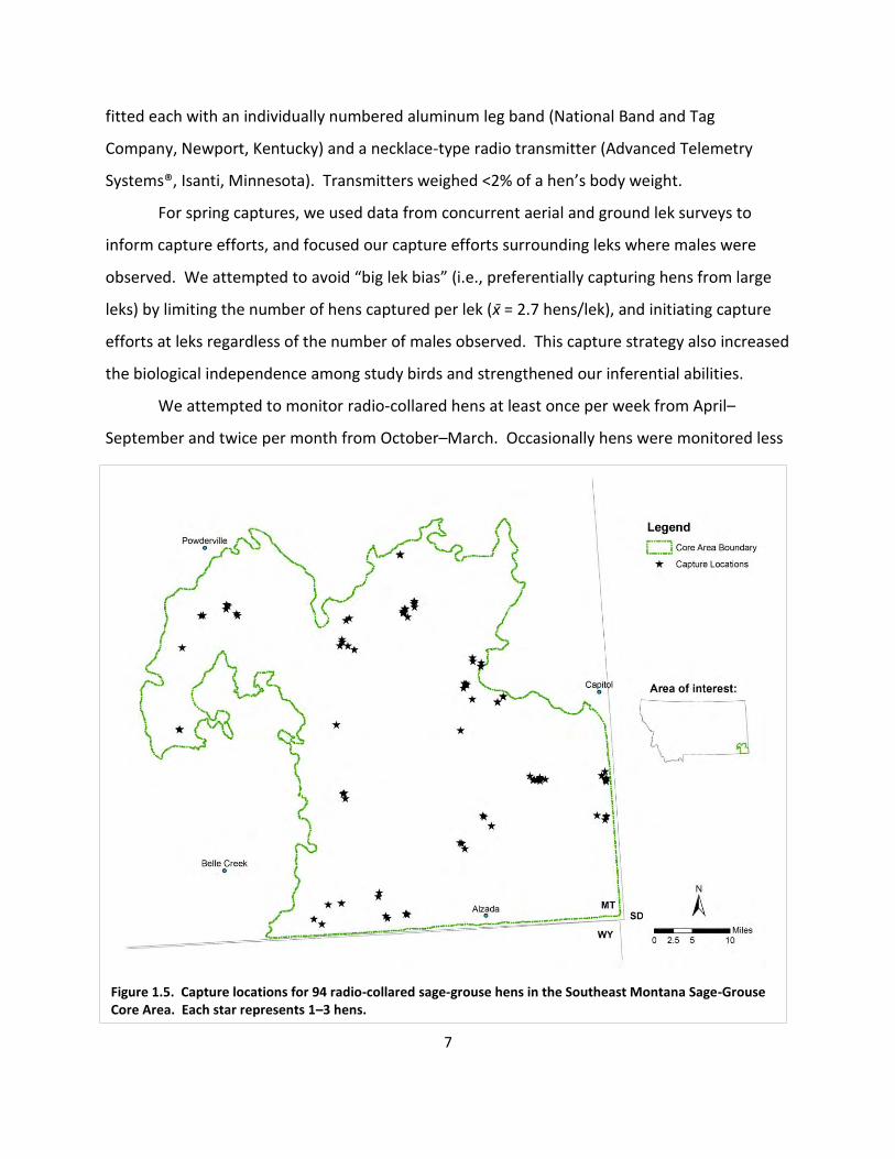
We captured a total of 94 sage-grouse hens between spring 2009 and spring 2012 (2009

= 12, 2010 = 54, 2011 = 27, 2012 = 1; Fig. 1.5). All hens were captured using the nighttime

spotlighting and hoop-netting technique (Wakkinen et al. 1992). We used plumage

characteristics to determine age for each hen (yearling or adult; Eng 1955, Crunden 1963), and

Figure 1.4. The Southeast Montana Sage-grouse Core Area contains large expanses of intact sagebrush-steppe habitat.

7

fitted each with an individually numbered aluminum leg band (National Band and Tag

Company, Newport, Kentucky) and a necklace-type radio transmitter (Advanced Telemetry

Systems®, Isanti, Minnesota). Transmitters weighed <2% of a hen’s body weight.

For spring captures, we used data from concurrent aerial and ground lek surveys to

inform capture efforts, and focused our capture efforts surrounding leks where males were

observed. We attempted to avoid “big lek bias” (i.e., preferentially capturing hens from large

leks) by limiting the number of hens captured per lek ( = 2.7 hens/lek), and initiating capture

efforts at leks regardless of the number of males observed. This capture strategy also increased

the biological independence among study birds and strengthened our inferential abilities.

We attempted to monitor radio-collared hens at least once per week from April–

September and twice per month from October–March. Occasionally hens were monitored less

Figure 1.5. Capture locations for 94 radio-collared sage-grouse hens in the Southeast Montana Sage-Grouse Core Area. Each star represents 1–3 hens.

8

frequently due to severe weather events or logistical constraints. We used telemetry homing

techniques (Samuel and Fuller 1996) to locate hens on the ground from April–September. We

conducted telemetry flights when hens could not be located on the ground and to locate all

hens from October–March. At each location, we recorded status (e.g., live, dead, nesting), GPS

location, habitat information, and other pertinent notes.

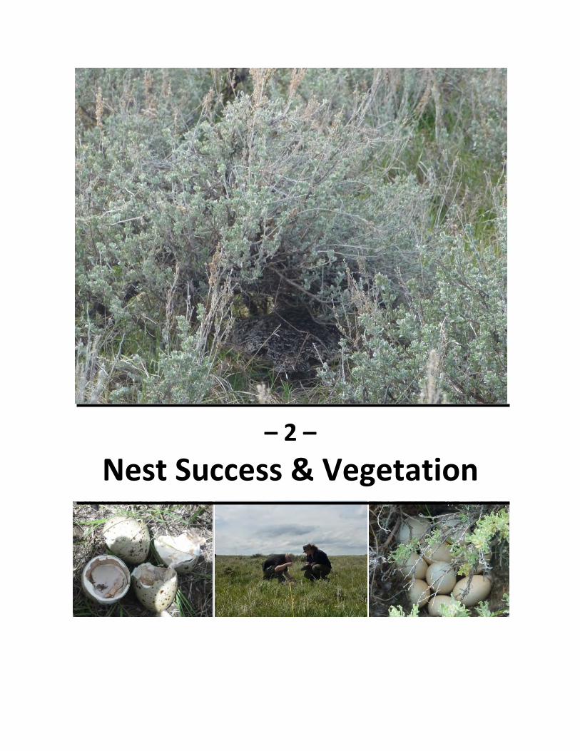
– 2 –

Nest Success & Vegetation

10

INTRODUCTION

Nest success is one of the most important parameters driving population growth rates

for sage-grouse (Taylor et al. 2010). Nest success varies among individual populations of sage-

grouse and years, and may be influenced by land management and development activities

(Connelly et al. 2011a). Therefore, it is necessary to quantify sage-grouse nest success and

identify factors that may influence or limit nest success within sage-grouse core areas in order

to better understand local population dynamics and make recommendations to improve nest

success.

Sage-grouse nest success may be influenced by a variety of factors that land managers

are unable to control such as climate, annual weather and existing levels of habitat

fragmentation and development. However, land managers may have the ability to influence

future land use and development activities. Two common practices to protect nesting sage-

grouse and improve nest success are vegetation management and restrictions on development

activities. Kevin Dougherty (University of Montana, unpublished data in Taylor et al. 2010)

demonstrated that a 2 inch increase in grass height could result in a 10% increase in nest

success, which could translate into an 8% increase in annual population growth (Taylor et al.

2010). Therefore, managed grazing is one of the few tools available for land managers to

improve rates of nest success and facilitate sage-grouse population growth (Taylor et al. 2010).

Timing restrictions to protect breeding and nesting sage-grouse from disturbance due to noise

and activity associated with development typically begin March 1 and end June 15, but nesting

season dates vary among sage-grouse populations (Schroeder et al. 1999, Gregg 2006).

Therefore, quantifying nesting season dates and adjusting timing restrictions accordingly may

minimize impacts of development on nesting grouse, as long as development activities do not

result in long-term habitat loss, fragmentation, or degradation.

We quantified nesting season dates, nesting vital rates (nest initiation and success),

fates of failed nests, nest site vegetation, and livestock occurrence at nest sites. We also

investigated the influence of vegetation, livestock occurrence, weather, and other factors (e.g.,

hen age) on sage-grouse nest success. The resulting information will allow managers to better

understand sage-grouse nest success within the Core Area (Fig. 1.2), identify factors that

11

influence success, and make appropriate management recommendations. It also provides

valuable site-specific baseline data for comparison with other studies and the Core Area in the

future.

METHODS

Nest monitoring

We monitored nests each spring from 2010–2012. We tracked hens at least once

weekly using radiotelemetry equipment to locate nests and visually confirmed that hens were

nesting from a distance of 15–20 yards. We estimated incubation initiation for each nest as the

middle date between the last observation of a hen off a nest and the first observation of the

same hen on a nest. For 8 nests with a long interval between observations (e.g., if a hen could

not be located and was later found on a nest), we flushed hens and floated eggs to estimate

incubation stage based on a 27 day incubation period (Westerkov 1950, Schroeder et al. 1999).

This technique was necessary to accurately calculate dates for incubation initiation, but may

cause some hens to abandon nests (Moynahan et al. 2007, Connelly et al. 2011a). Thus, we

revisited flushed hens the following day to ensure that any researcher-caused nest

abandonment was detected; no hens abandoned nests due to this technique. Once incubation

was confirmed, we monitored nests at least weekly from >75 yards until hatch or nest failure.

We classified failed nests as depredated (empty/destroyed nest bowl or hen dead) or

abandoned (clutch intact and hen alive). We considered nests successful if at least one egg

hatched determined by the presence of eggshells with detached membranes (Klebenow 1969).

When nest bowls were undisturbed following a successful hatch, we counted the clutch size.

We also noted whether livestock were present in the pasture where the nest occurred.

Vegetation sampling

We quantified vegetation structure at and adjacent to nest locations using protocol

consistent with sage-grouse research elsewhere (e.g., Connelly et al. 2000b, Hagen et al. 2007,

C. Wambolt, Montana State University, unpublished). We quantified shrub and herbaceous

12

vegetation structure along 2 perpendicular 98-ft line transects centered on nest bowls running

from north to south and from east to west. We recorded the species, height, and maximum

width of nest shrubs. We measured canopy cover of live shrubs using the line-intercept

method (Canfield 1941, Connelly et al. 2003). We calculated shrub density by counting shrubs

>6 inches in crown width within 3.3-ft of transects. We also measured the height of the nearest

shrub at 3.3-ft intervals along the transect line. We measured herbaceous horizontal cover by

placing 8 x 16 inch frames (Daubenmire 1959) at 10-ft intervals along line transects and

recorded the percent cover (<5%, 5–25%, 25–50%, 50–75%, 75–95% or >95%) of 5 cover classes

(live grass, residual vegetation, forb, cactus, and bare ground). We also measured the

maximum live grass, forb, and the height of residual herbaceous vegetation within frames

(residual height was only measured in 2011 and 2012). We measured visual obstruction at nest

bowls by collecting height-density readings in each cardinal direction 13 ft from the nest bowl

at a height of 3.3 ft following Robel et al. (1970).

Analyses

To evaluate the effectiveness of timing restrictions designed to benefit nesting hens, we

present the median incubation initiation date and the length of the nesting season for each

year of the study. We also present the median incubation initiation date of first nests by hen

age class (yearling vs. adult). To better understand sage-grouse population dynamics within the

Core Area and for comparison with other studies, we calculated several nesting vital rates. We

calculated: 1) nest and renest initiation rates for each age class (yearling and adult) and year of

the study, 2) mean, SE, and range for nest and renest clutch size, 3) apparent nest success

(successful nests/all nest attempts) for each age class and nest attempt each year and overall

apparent nest success for each year. Apparent nest success is useful for comparison with other

studies, but is subject to bias (Mayfield 1961, Mayfield 1975). Maximum-likelihood estimators

of daily survival rate are preferred to analyze nest survival data (Rotella 2010). We calculated

the maximum-likelihood estimates for nest success using daily survival rate (DSR) of nests

generated using program MARK (Rotella 2010) and a 27 day incubation period (Westerkov

1950, Schroeder et al. 1999). We present the percent of nests where livestock use was

13

concurrent with nesting and compared apparent nest success between nests in pastures with

and without livestock present. We censored 2 nests from success analyses because we

suspected researchers contributed to their failure. We also present fates of failed nests.

We provide descriptive information for nest site vegetation. For each nest shrub and

stand variable, we calculated mean, SE, and range. The quantity and composition of

herbaceous vegetation varies annually with precipitation. Therefore, we tested for differences

in live grass height, forb height, and visual obstruction at nest sites among years using analysis

of variance (ANOVA) and Tukey’s honestly significant difference (HSD) multiple comparison test

(α = 0.05). We used a t-test to test for differences in the height of residual herbaceous

vegetation between years (α = 0.05). We present horizontal cover (mean and SE for each cover

class) separately for each year. We used topography data in GIS to calculate the mean, SE, and

range of elevation at nest locations.

We used an information-theoretic approach and the corrected Akaike Information

Criterion (AICc; Burnham and Anderson 2002) to test among competing models for daily nest

survival (DSR) in program MARK. We were interested in assessing 1) vegetation characteristics

important for nest survival, 2) whether livestock presence influenced nest success, 3) if nest

survival was related to local weather (average temperature and average daily rainfall during the

nest survival period gathered from station USC00247034, NOAA, Ridgeway, MT), and 4)

differences in nest survival between age classes. We also tested models for different nest

success among years, nest attempt (first nest or renest), and calendar date. We compared all

models against the null model of a constant DSR.

RESULTS

Nesting season dates

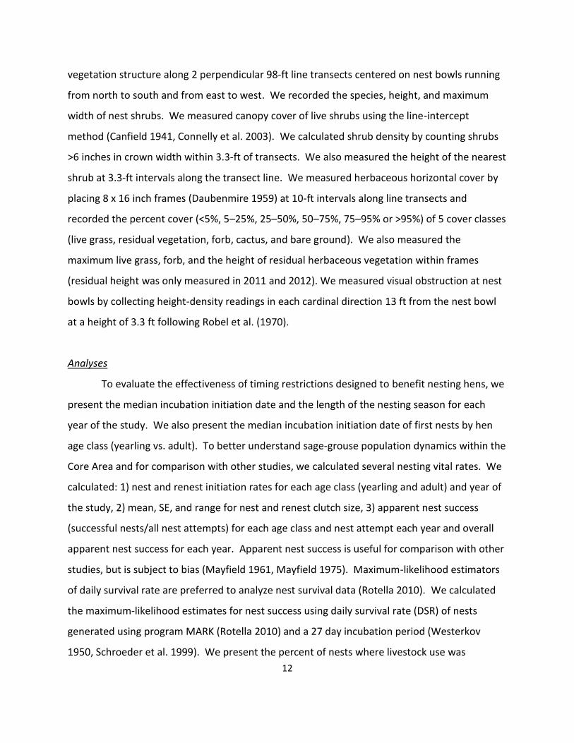
The median incubation initiation date (first nests and renests combined) was 2–3 weeks

earlier in 2012 than 2010 or 2011 (Table 2.1). The total nesting season length, beginning with

the earliest incubation initiation to the last hatch/depredation date, was similar in 2010 and

2011 (approximately 80 days), but shorter in 2012 (approximately 60 days; Table 2.1). The

14

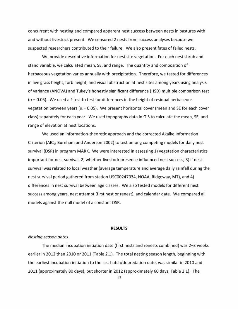
Table 2.2. Percent of radio-collared sage-grouse hens that initiated a first nest and renested by age class and year.

% Nest Initiation % Renest

Yearling 87% (80/86) 21% (5/24)

Adult

93% (34/39) 52% (23/42)

2010 87% (48/55) 40% (12/30)

2011 100% (43/43) 48% (13/27)

2012

85% (23/27) 29% (2/7)

Overall 91% (114/125) 42% (27/64)

nesting season began in mid-April each year, but lasted approximately a month longer in 2010

and 2011 than 2012 (Table 2.1). Yearling hens initiated first nests about a week later than adult

hens in both 2010 and 2011 (adult median = 4/30/10 and 5/5/11; yearling median = 5/7/10 and

5/13/11). There were no yearlings in the study in 2012.

Nesting vital rates

We summarized nesting results for 55

hens in 2010, 43 in 2011, and 27 in 2012. The

percent of hens that initiated a first nest was

variable but high for all years (≥85%; Table

2.2). The percent of hens (adult and yearling)

that renested following an unsuccessful first

nest was 42% across all years, although hens

in 2012 renested at a lower rate than 2010

and 2011 (Table 2.2). Overall, 93% of adult hens and 87% of yearlings initiated a first nest, and

52% of adult hens and 21% of yearlings renested (Table 2.2). Two adult hens initiated a 3rd nest

in 2011. Average clutch size was 7.92 eggs (SE = 0.16; range = 4–10) for first nests and 6.54

eggs (SE = 0.40; range = 4–9) for renests.

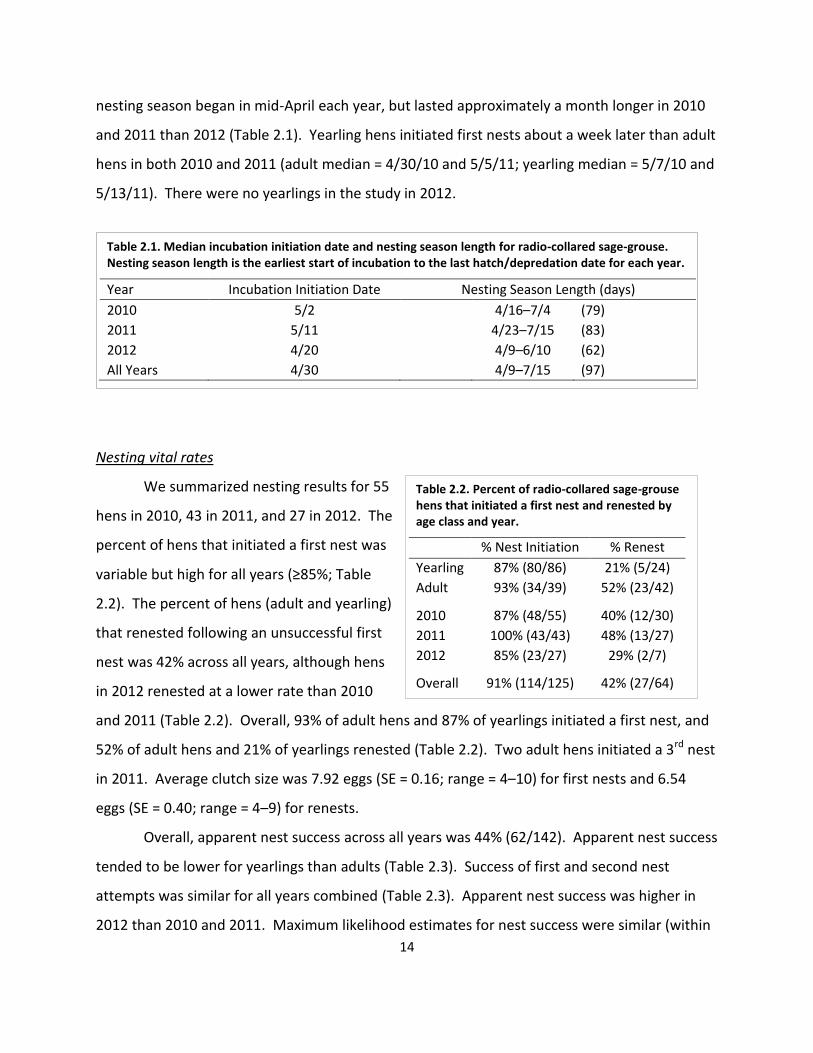
Overall, apparent nest success across all years was 44% (62/142). Apparent nest success

tended to be lower for yearlings than adults (Table 2.3). Success of first and second nest

attempts was similar for all years combined (Table 2.3). Apparent nest success was higher in

2012 than 2010 and 2011. Maximum likelihood estimates for nest success were similar (within

Table 2.1. Median incubation initiation date and nesting season length for radio-collared sage-grouse. Nesting season length is the earliest start of incubation to the last hatch/depredation date for each year.

Year Incubation Initiation Date Nesting Season Length (days)

2010 5/2 4/16–7/4 (79)

2011 5/11 4/23–7/15 (83)

2012 4/20 4/9–6/10 (62)

All Years 4/30 4/9–7/15 (97)

15

2%) to apparent nest success for 2010 and 2011, but 8% lower for 2012. Twenty-four percent

(34/142) of nests were in pastures with cattle, 2% (4/142) with sheep, and 1% (2/142) with both

cattle and sheep present. Apparent nest success was higher for nests in pastures with livestock

present (59%; 24/41) than nests in pastures without livestock (38%; 38/100).

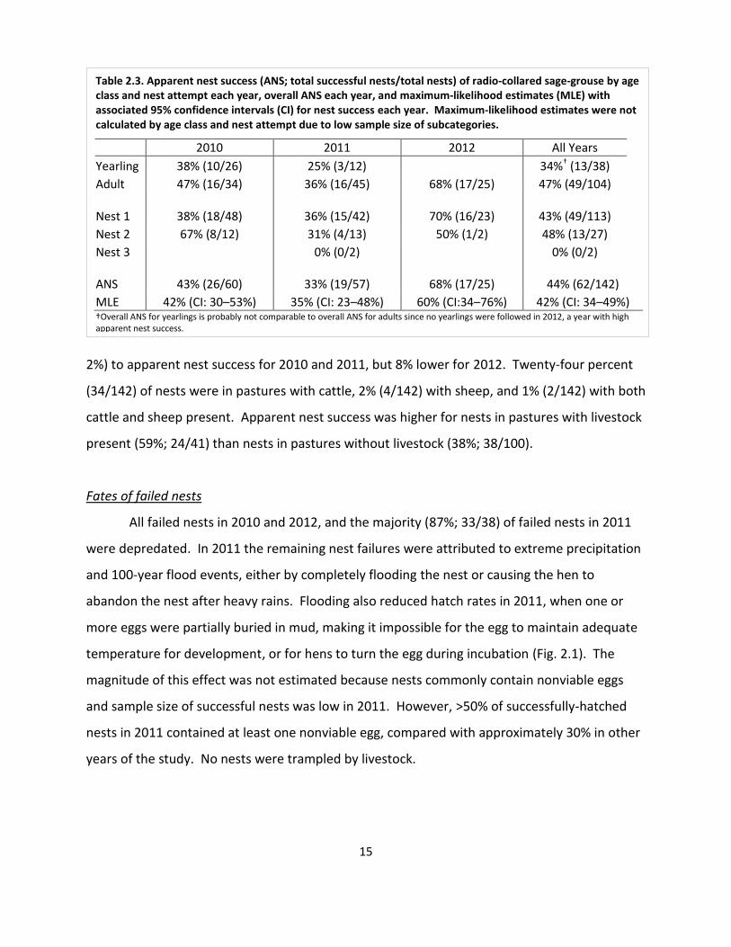
Fates of failed nests

All failed nests in 2010 and 2012, and the majority (87%; 33/38) of failed nests in 2011

were depredated. In 2011 the remaining nest failures were attributed to extreme precipitation

and 100-year flood events, either by completely flooding the nest or causing the hen to

abandon the nest after heavy rains. Flooding also reduced hatch rates in 2011, when one or

more eggs were partially buried in mud, making it impossible for the egg to maintain adequate

temperature for development, or for hens to turn the egg during incubation (Fig. 2.1). The

magnitude of this effect was not estimated because nests commonly contain nonviable eggs

and sample size of successful nests was low in 2011. However, >50% of successfully-hatched

nests in 2011 contained at least one nonviable egg, compared with approximately 30% in other

years of the study. No nests were trampled by livestock.

Table 2.3. Apparent nest success (ANS; total successful nests/total nests) of radio-collared sage-grouse by age class and nest attempt each year, overall ANS each year, and maximum-likelihood estimates (MLE) with associated 95% confidence intervals (CI) for nest success each year. Maximum-likelihood estimates were not calculated by age class and nest attempt due to low sample size of subcategories.

2010 2011 2012 All Years

Yearling 38% (10/26) 25% (3/12)

34%† (13/38)

Adult 47% (16/34) 36% (16/45) 68% (17/25) 47% (49/104) Nest 1 38% (18/48) 36% (15/42) 70% (16/23) 43% (49/113)

Nest 2 67% (8/12) 31% (4/13) 50% (1/2) 48% (13/27)

Nest 3

0% (0/2)

0% (0/2) ANS 43% (26/60) 33% (19/57) 68% (17/25) 44% (62/142)

MLE 42% (CI: 30–53%) 35% (CI: 23–48%) 60% (CI:34–76%) 42% (CI: 34–49%) †Overall ANS for yearlings is probably not comparable to overall ANS for adults since no yearlings were followed in 2012, a year with high apparent nest success.

16

Nest vegetation

Ninety percent (128/143) of nests were located beneath Wyoming big sagebrush, 7

nests were located in herbaceous vegetation with no shrub present, 4 nests beneath silver

sagebrush, 3 beneath greasewood, and 1 nest beneath a silver buffaloberry (Sherpherdia

argentea). Nest shrub and stand characteristics are presented in Table 2.4. Average grass

height (f2,140 = 31.94, P < 0.001) and average forb height (f2,139 = 45.47, P < 0.001) differed

among years and were lowest in 2012. The average height of residual herbaceous vegetation

was greater in 2012 than 2011 (t43 = 2.02, P = 0.01; Table2.3). No differences were detected in

visual obstruction (f2,139 = 0.01, P = 0.99) at nest bowls among years (Table 2.4). Horizontal

cover at nest stands was dominated by residual vegetation and bare ground in all years, but live

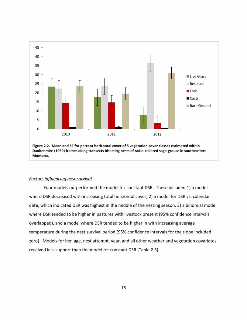
grass and forb cover were higher in 2010 and 2011 than 2012 (Figure 2.2). Nest sites were

located at an average elevation of 3442 ft (SE = 15 ft; range 2933–3907 ft).

Figure 2.1. Nearly all nest failures were a result of depredation (left photo). However, a 100-year flood event in 2011 caused 9% of nests to fail and reduced the hatch rate for many nests when one or more eggs were partially buried in mud, making it impossible for the egg to maintain adequate temperature for development (right photo). The egg in the foreground of the photo on the right successfully hatched, but the 3 eggs behind did not.

17

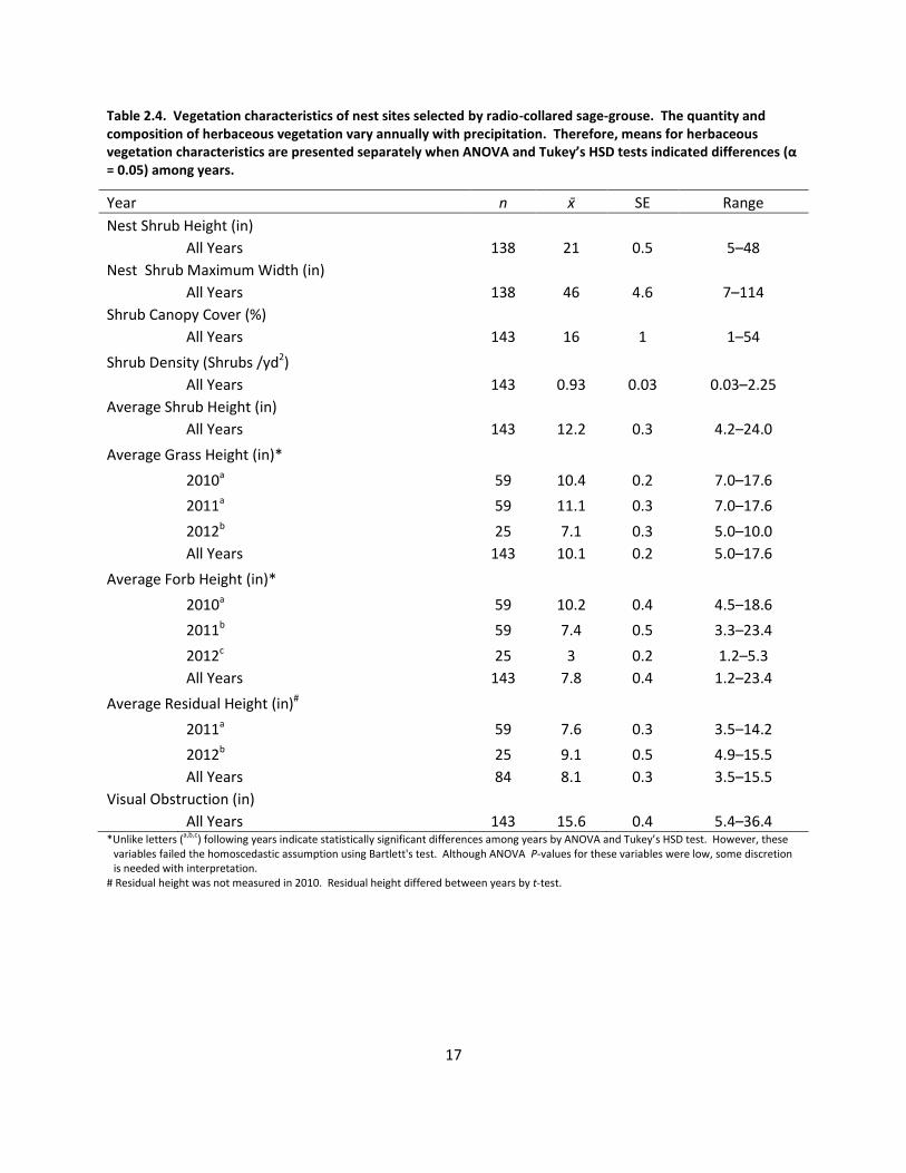
Table 2.4. Vegetation characteristics of nest sites selected by radio-collared sage-grouse. The quantity and composition of herbaceous vegetation vary annually with precipitation. Therefore, means for herbaceous vegetation characteristics are presented separately when ANOVA and Tukey’s HSD tests indicated differences (α = 0.05) among years.

Year n SE Range

Nest Shrub Height (in)

All Years 138 21 0.5 5–48

Nest Shrub Maximum Width (in)

All Years 138 46 4.6 7–114

Shrub Canopy Cover (%)

All Years 143 16 1 1–54

Shrub Density (Shrubs /yd2)

All Years 143 0.93 0.03 0.03–2.25

Average Shrub Height (in)

All Years 143 12.2 0.3 4.2–24.0

Average Grass Height (in)*

2010a 59 10.4 0.2 7.0–17.6

2011a 59 11.1 0.3 7.0–17.6

2012b 25 7.1 0.3 5.0–10.0

All Years 143 10.1 0.2 5.0–17.6

Average Forb Height (in)*

2010a 59 10.2 0.4 4.5–18.6

2011b 59 7.4 0.5 3.3–23.4

2012c 25 3 0.2 1.2–5.3

All Years 143 7.8 0.4 1.2–23.4

Average Residual Height (in)#

2011a 59 7.6 0.3 3.5–14.2

2012b 25 9.1 0.5 4.9–15.5

All Years 84 8.1 0.3 3.5–15.5

Visual Obstruction (in)

All Years 143 15.6 0.4 5.4–36.4 *Unlike letters (a,b,c) following years indicate statistically significant differences among years by ANOVA and Tukey’s HSD test. However, these

variables failed the homoscedastic assumption using Bartlett's test. Although ANOVA P-values for these variables were low, some discretion is needed with interpretation.

# Residual height was not measured in 2010. Residual height differed between years by t-test.

18

Factors influencing nest survival

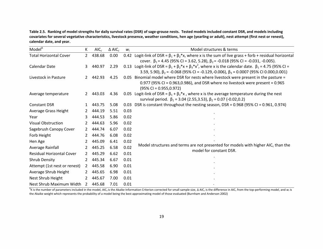
Four models outperformed the model for constant DSR. These included 1) a model

where DSR decreased with increasing total horizontal cover, 2) a model for DSR vs. calendar

date, which indicated DSR was highest in the middle of the nesting season, 3) a binomial model

where DSR tended to be higher in pastures with livestock present (95% confidence intervals

overlapped), and a model where DSR tended to be higher in with increasing average

temperature during the nest survival period (95% confidence intervals for the slope included

zero). Models for hen age, nest attempt, year, and all other weather and vegetation covariates

received less support than the model for constant DSR (Table 2.5).

Figure 2.2. Mean and SE for percent horizontal cover of 5 vegetation cover classes estimated within Daubenmire (1959) frames along transects bisecting nests of radio-collared sage-grouse in southeastern Montana.

0

5

10

15

20

25

30

35

40

45

2010 2011 2012

Live Grass

Residual

Forb

Cacti

Bare Ground

19

Table 2.5. Ranking of model strengths for daily survival rates (DSR) of sage-grouse nests. Tested models included constant DSR, and models including covariates for several vegetative characteristics, livestock presence, weather conditions, hen age (yearling or adult), nest attempt (first nest or renest), calendar date, and year.

ModelA K AICc Δ AICc wi Model structures & terms

Total Horizontal Cover 2 438.68 0.00 0.42 Logit-link of DSR = β1 + β2*x, where x is the sum of live grass + forb + residual horizontal cover. β1 = 4.45 (95% CI = 3.62, 5.28), β2 = -0.018 (95% CI = -0.031, -0.005).

Calendar Date 3 440.97 2.29 0.13 Logit-link of DSR = β1 + β2*x + β3*x2, where x is the calendar date. β1 = 4.75 (95% CI = 3.59, 5.90), β2 = -0.068 (95% CI = -0.129,-0.006), β3 = 0.0007 (95% CI 0.000,0.001)

Livestock in Pasture 2 442.93 4.25 0.05 Binomial model where DSR for nests where livestock were present in the pasture = 0.977 (95% CI = 0.963,0.986), and DSR where no livestock were present = 0.965 (95% CI = 0.955,0.972)

Average temperature 2 443.03 4.36 0.05 Logit-link of DSR = β1 + β2*x , where x is the average temperature during the nest survival period. β1 = 3.04 (2.55,3.53), β2 = 0.07 (-0.02,0.2)

Constant DSR 1 443.75 5.08 0.03 DSR is constant throughout the nesting season, DSR = 0.968 (95% CI = 0.961, 0.974)

Average Grass Height 2 444.19 5.51 0.03 . . . . . .

Model structures and terms are not presented for models with higher AICc than the model for constant DSR.

.

.

.

.

. .

Year 3 444.53 5.86 0.02

Visual Obstruction 2 444.63 5.96 0.02

Sagebrush Canopy Cover 2 444.74 6.07 0.02

Forb Height 2 444.76 6.08 0.02

Hen Age 2 445.09 6.41 0.02

Average Rainfall 2 445.25 6.58 0.02

Residual Horizontal Cover 2 445.29 6.62 0.01

Shrub Density 2 445.34 6.67 0.01

Attempt (1st nest or renest) 2 445.58 6.90 0.01

Average Shrub Height 2 445.65 6.98 0.01

Nest Shrub Height 2 445.67 7.00 0.01

Nest Shrub Maximum Width 2 445.68 7.01 0.01 AK is the number of parameters included in the model, AICc is the Akaike Information Criterion corrected for small sample size, Δ AICc is the difference in AICc from the top-performing model, and wi is the Akaike weight which represents the probability of a model being the best approximating model of those evaluated (Burnham and Anderson 2002)

DISCUSSION

The nesting season was much shorter in 2012 (62 days) than 2010 and 2011 (≥79 days),

due to high success of first nests and few renesting attempts. We attributed the difference

primarily to drought conditions in 2012 (Appendix A). The lack of yearlings in the study during

2012 may have also contributed to a shorter nesting season, since yearlings tended to initiate

first nests about a week later than adults. Similarly, the median incubation initiation date in

2012 (April 20) was nearly 2 weeks earlier than 2010 (May 2) and 3 weeks earlier than 2011

(May 11), and the nesting season lasted into early/mid-July during 2010 and 2011 but was

complete by June 10 in 2012. Therefore, timing restrictions to benefit nesting grouse that end

on June 15 may be effective during dry years, but during wetter years or years with a

protracted nest season, the median start date for incubation is early to mid-May, and therefore

only about 50% of nests would be expected to hatch by mid-June.

Nest initiation rates were higher in all years in the Core Area (Table 2.2; = 91%) than

averages from the eastern range of sage-grouse (82%, range = 67–100%; reviewed in Connelly

et al. 2011a). Yearlings and adults had similar rates of initiation for first nests (87% and 93%,

respectively), unlike studies elsewhere that documented lower nest initiation rates for yearlings

(Connelly et al. 1993, Holloran et al. 2005, Moynahan et al. 2007). Conversely, yearlings had a

much lower renesting probability than adults (23% and 52%, respectively). Others have

suggested this may be due to later dates of first nest initiation for yearlings (Coggins 1998,

Schroeder 1997, Moynahan et al. 2007). Overall, hens during the study had a higher renesting

probability (42%) than the eastern range average (20%, range 9–38%; reviewed in Connelly et

al. 2011a), even during 2012 when renesting rates were lowest (29%) during the study. High

rates of nest and renest initiation in 2010 and 2011 may have been driven by above-average

spring precipitation (Appendix A) which contributed to a long nesting season (79 and 83 days,

respectively) and provided an abundance of protein-rich insects and forbs necessary for clutch

production (Barnett and Crawford 1994, Coggins 1998, Gregg et al. 2006, Moynahan et al.

2007). Conversely, nest and renest initiation rates were lowest during drought year 2012

(Appendix A).

21

The average clutch size (7.6 eggs) was similar to that of nests from the eastern portion

of the sage-grouse range (7.5 eggs; reviewed in Connelly et al. 2011a), northcentral Montana

(8.3 eggs; Moynahan et al. 2007), northwestern South Dakota (8.3 eggs; Kaczor 2008), and

southwest North Dakota (7.9 eggs; Herman-Brunson et al. 2009). Despite consistent clutch

sizes produced, hatch rates were depressed in 2011 due to flood conditions. Extreme

precipitation in 2011 caused some eggs to become partially buried in mud, making it impossible

for eggs to maintain adequate temperature for development.

Apparent nest success varied among years (43% in 2010, 33% in 2011, and 68% in 2012).

Maximum-likelihood estimates followed a similar trend, but 95% confidence intervals

overlapped for all years (Table 2.3) and the model for different DSR among years performed

poorly (Table 2.5). Low nest success in 2011 was driven by extreme precipitation and 100-year

flood events, which caused 9% of nests to fail. Nest success is generally higher in wetter years

(Coggins 1998, Gregg et al. 2006, Moynahan et al. 2007), but we suspect that flooding coupled

with periods of below-average temperature in springs 2010 and 2011 (Appendix A) may have

limited nest success in both years. However, the model for average daily rainfall performed

poorly (Table 2.5), perhaps because rainfall has both positive (e.g., vegetation growth) and

negative (e.g., flooding) effects that may have complex interactions with the nest site (e.g.,

topography at the nest site) or pattern of rainfall (e.g., gentle rain overnight versus a quick

downpour). Also, rainfall is generally accompanied by cooler temperatures which may affect

nest survival. We observed a trend for increasing DSR with increasing average temperature

during the nest survival period, but 95% confidence intervals about the slope (β2) overlapped

zero (Table 2.5).

Vegetation, especially sagebrush canopy cover, residual vegetation, and live grass

growth, is a primary factor that impacts sage-grouse nest success (e.g., Gregg et al. 1994,

Connelly et al. 2000b, Holloran et al. 2005, Rebholz et al. 2009, Coates and Delehanty 2010), yet

models relating nest shrub and stand characteristics to nest survival generally performed poorly

(Table 2.5). The only vegetative model that outperformed the model for constant DSR was the

sum of live grass + forb + residual horizontal cover. However, the slope of the resulting

equation was negative, and solving the equation indicates that 5% increase in cover would

22

result in a 3% decrease in nest success. We suspect this counterintuitive outcome is a type II

error. However, these results are a strong indication that herbaceous and shrub cover did not

limit nest success during the study. Extreme moisture in 2010–11 resulted in tremendous

growth of live vegetation, and abundant residual cover during 2012 (Table 2.4; Figure 2.2).

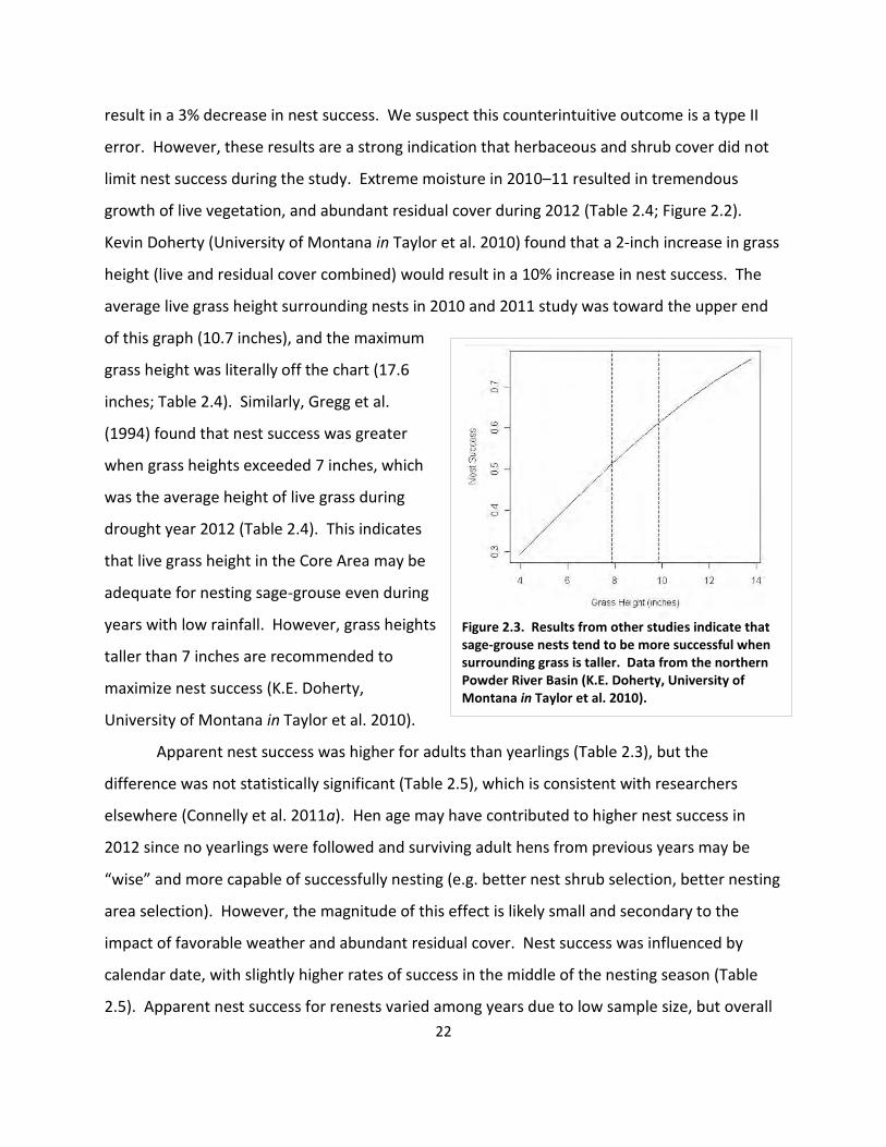
Kevin Doherty (University of Montana in Taylor et al. 2010) found that a 2-inch increase in grass

height (live and residual cover combined) would result in a 10% increase in nest success. The

average live grass height surrounding nests in 2010 and 2011 study was toward the upper end

of this graph (10.7 inches), and the maximum

grass height was literally off the chart (17.6

inches; Table 2.4). Similarly, Gregg et al.

(1994) found that nest success was greater

when grass heights exceeded 7 inches, which

was the average height of live grass during

drought year 2012 (Table 2.4). This indicates

that live grass height in the Core Area may be

adequate for nesting sage-grouse even during

years with low rainfall. However, grass heights

taller than 7 inches are recommended to

maximize nest success (K.E. Doherty,

University of Montana in Taylor et al. 2010).

Apparent nest success was higher for adults than yearlings (Table 2.3), but the

difference was not statistically significant (Table 2.5), which is consistent with researchers

elsewhere (Connelly et al. 2011a). Hen age may have contributed to higher nest success in

2012 since no yearlings were followed and surviving adult hens from previous years may be

“wise” and more capable of successfully nesting (e.g. better nest shrub selection, better nesting

area selection). However, the magnitude of this effect is likely small and secondary to the

impact of favorable weather and abundant residual cover. Nest success was influenced by

calendar date, with slightly higher rates of success in the middle of the nesting season (Table

2.5). Apparent nest success for renests varied among years due to low sample size, but overall

Figure 2.3. Results from other studies indicate that sage-grouse nests tend to be more successful when surrounding grass is taller. Data from the northern Powder River Basin (K.E. Doherty, University of Montana in Taylor et al. 2010).

23

was similar to success for first nests (Table 2.3, Table 2.5), which differs from research

conducted in central Montana where DSR was higher for renesting attempts than first nests

(Sika 2006).

Overall apparent nest success for hens in the Core Area (43%) was similar to the average

across the sage-grouse range (46%, range = 15–86%), but lower than the average for non-

altered habitats (51%, range 24–71%; reviewed in Connelly et al. 2011a). Although extreme

weather occurred during all years of the study, 2011 presented the most extreme conditions

during the nesting season. In 2011, a 100-year flood event occurred during the nesting season

that had a myriad of direct and indirect negative effects on nests and hens. Therefore, it may

be reasonable to assume that average nest success in the Core Area would be more accurately

estimated by averaging maximum-likelihood estimates for 2010 (42%; a cold, wet nesting

season) and 2012 (60%; a warm, dry nesting season), while censoring nest success from

extreme 2011. This results in 51% average nest success, which is equal to the average for

unaltered habitats and probably a realistic estimate since the Core Area consists of largely

intact habitat (Taylor et al. 2010).

Flooding drove between-year differences in apparent nest success, but depredation was

the primary cause of nest failure in every year of the study. It is impossible to reliably assign a

nest predator to species or class (e.g., aves or mammalia) based on sign left at the nest bowl

(Coates et al. 2008). Potential nest predators that were observed in the study area include red

fox (Vulpes vulpes), American badger (Taxidea taxus), bobcat (Felis rufus), coyote (Canis

latrans), striped skunk (Memphitis memphitis), raccoon (Procyon lotor), domestic cat, common

raven (Corvus corax), American crow (Corvus brachyrhynchos), and a variety of snake species.

We suspect American badgers and striped skunks were responsible the majority of nest

depredations. Both species were commonly observed during nighttime radio collaring efforts in

the Core Area, and striped skunks followed by American badger were the most prevalent

wildlife species observed at camera stations in a concurrent study in the Core Area (J.

Alexander, St. Cloud State University, unpublished data). Common ravens and American crows

do occur in the Core Area and potentially could have depredated some nests, but their

abundance is low (based on field observations) and we suspect they were minor contributors to

24

nest predation. Although the majority of nest failures were due to predation, we do not

presume that nest predation is a limiting factor for grouse within the Core Area because 1) for

sage-grouse, as with other ground nesting birds, nest predation is a normal and expected

occurrence, and 2) observed rates of nest success during our study were comparable with

healthy sage-grouse populations elsewhere.

Maximum-likelihood models indicated a trend for increased DSR for nests in pastures

with livestock present concurrent with the nest, and apparent nest success was higher for nests

in pastures with livestock (59%) than pastures without livestock (38%). Additionally, we

observed no direct negative impacts (e.g., trampling of nests) of livestock on nesting grouse. A

similar trend has occasionally been reported for other prairie nesting birds. For example, Kirby

and Grosz (1995) reported 25% higher nest success for sharp-tailed grouse (Tympanuchus

phasianellus) in grazed than ungrazed pastures and Barker et al. (1990) reported 24% higher

nest success for waterfowl nesting in twice-over rotationally-grazed pastures than idle pastures.

Kirby and Grosz (1995) suggested this effect may have been a the result of behavioral

avoidance of livestock by predators, or that grazing pastures reduced cover for predators, and

that conversely the seclusion and cover provided by ungrazed areas may attract greater

numbers of nest predators. Higher nest success in pastures with livestock may also reflect

predator control efforts in areas with livestock, or predators focusing on alternate food sources

(e.g., afterbirth) in areas with livestock. This effect was probably not an artifact of ranchers

turning cattle into pastures that contain the best cover early in the season, because our results

indicated that nest success was not related to vegetative characteristics. Regardless of the

mechanism, a trend for higher nest success in grazed pastures coupled with no indication of

vegetation structure limiting nest success are strong indicators that ranching activities that are

occurring in the Core Area are not detrimental to nesting grouse. Overall, results from our

study concur with research elsewhere that managed grazing is compatible with sage-grouse

conservation, but we caution that we did not rigorously quantify the complex interrelationships

among grazing, vegetation and sage-grouse nest success.

- 3 -

Brood Success & Vegetation

26

INTRODUCTION

Chick survival during the early brood-rearing period is one of the most influential and

most variable population parameters for sage-grouse (Gregg et al. 2007, Connelly et al. 2011b,

Taylor et al. 2012). Taylor et al. (2012) demonstrated that chick survival is the second most

influential vital rate, behind hen survival, that influences population growth rates for sage-

grouse, and that chick survival may account for >22% of the variation in population growth

rates. Chick survival rates range from 12–50% for the first 18–51 days post-hatch and brood

success (the percent of successfully-hatched broods where ≥1 chick survives past the early

brood-rearing period) ranges from 21–100% (reviewed in Sika 2006). One reason for this

variability is that chick survival is highly dependent on weather conditions. Young chicks (<2

weeks old) cannot thermoregulate independently and may succumb to exposure during cold,

wet weather (Patterson 1952, Wallestad 1975). Further, chick survival is heavily influenced by

forage (forbs and insects) availability and cover from predators, both of which are influenced by

the timing and amount of precipitation. Although land managers cannot control precipitation,

they can influence forage and cover available for brood-rearing sage-grouse through land

management practices (e.g., grazing prescriptions) that improve vegetation structure and

composition.

In order to improve our understanding of local sage-grouse population dynamics and

make recommendations to improve chick survival rates, our objectives were to quantify brood-

rearing dates, vital rates, brood site vegetation, and livestock occurrence at brood-rearing sites.

The resulting information will allow managers to better understand sage-grouse brood success

within the Core Area (Fig. 1.2), identify factors that influence success, and make appropriate

management recommendations. It also provides valuable site-specific baseline data for

comparison with other studies and the Core Area in the future.

27

METHODS

Brood monitoring

We monitored brood success at 14 and 30 days post-hatch. We conducted daytime

flush counts at 14 days post-hatch and considered the brood successful if at least one chick was

observed or hen behavior (e.g., vocalizing and walking off rather than flushing) suggested chicks

were present. Broods were assumed failed if hens were observed with other breeding-aged

birds on or before 14 days post-hatch. When brood presence was uncertain at 14 days, we

returned at night when chicks roost with the hen to verify brood status. We did not attempt to

get accurate brood counts at 14 days because 1) sage-grouse chicks are difficult to detect in

daytime flush counts (Huwer 2004), and 2) two week old chicks were often fully concealed by

brood hens at night (Fig. 3.1). We conducted nighttime brood counts 30 days post-hatch. At

this point, chicks can be accurately counted since they are large enough that they cannot be

fully concealed beneath the hen.

Figure 3.1. Left: this hen is brooding several chicks; 2 week old chicks were often fully concealed underneath brood hens at night. Right: as chicks approach 30 days old, they are too large to be fully concealed beneath the hen and can be accurately counted during nighttime brood counts.

28

Brood site vegetation

We quantified habitat characteristics at brood locations 14, 21, and 30 days post-hatch

using 33-yd north to south transects centered on the brood location. We measured shrub

canopy cover, shrub density, shrub height, grass height, forb height, height of residual

herbaceous vegetation, horizontal cover, and livestock presence using vegetation sampling

methods described in Chapter 2. Forb species richness and composition may be important for

young chicks (Peterson 1970). Therefore, we determined the percent cover of each forb

species within Daubenmire (1959) frames placed at every other 3.3-yd mark (e.g. 3.3, 9.9, 16.6

yd) along transects. To avoid disturbing broods, we delayed vegetation sampling until the next

visit when hens and chicks had moved to a different location (within one week).

Analyses

We present the median and range of hatch dates for each year, and the percent of

broods that hatched after June 15 (a common end date for timing restrictions). We calculated

brood success and the average number of chicks per brood each year. We calculated chick

survival by dividing the number of chicks that survived to 30 days by the number of eggs

hatched. When nests were disturbed following hatch and it was impossible to accurately count

the number of eggs that successfully hatched, we used the average number of viable eggs from

other nests or renests as a surrogate. We calculated average chick production per hen by

dividing the number of chicks that survived to 30 days by the number of hens that entered the

nesting season.

We provide descriptive summaries of vegetation characteristics at brood locations.

Because 14 and 21-day brood locations were determined during the day (foraging locations)

and 30-day locations were determined at night (roosting locations), we report vegetation

characteristics separately if daytime and nighttime locations differed by t-test for each variable.

The quantity and composition of herbaceous vegetation varies annually with precipitation.

Therefore, we tested for differences in live grass height and forb height at brood sites among

years using analysis of variance (ANOVA) and Tukey’s honestly significant difference (HSD)

multiple comparison test. We used a t-test to test for differences in the height of residual

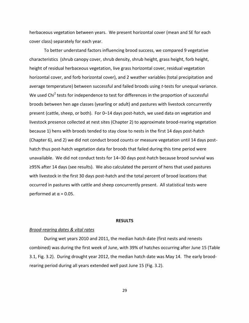
29

herbaceous vegetation between years. We present horizontal cover (mean and SE for each

cover class) separately for each year.

To better understand factors influencing brood success, we compared 9 vegetative

characteristics (shrub canopy cover, shrub density, shrub height, grass height, forb height,

height of residual herbaceous vegetation, live grass horizontal cover, residual vegetation

horizontal cover, and forb horizontal cover), and 2 weather variables (total precipitation and

average temperature) between successful and failed broods using t-tests for unequal variance.

We used Chi2 tests for independence to test for differences in the proportion of successful

broods between hen age classes (yearling or adult) and pastures with livestock concurrently

present (cattle, sheep, or both). For 0–14 days post-hatch, we used data on vegetation and

livestock presence collected at nest sites (Chapter 2) to approximate brood-rearing vegetation

because 1) hens with broods tended to stay close to nests in the first 14 days post-hatch

(Chapter 6), and 2) we did not conduct brood counts or measure vegetation until 14 days post-

hatch thus post-hatch vegetation data for broods that failed during this time period were

unavailable. We did not conduct tests for 14–30 days post-hatch because brood survival was

≥95% after 14 days (see results). We also calculated the percent of hens that used pastures

with livestock in the first 30 days post-hatch and the total percent of brood locations that

occurred in pastures with cattle and sheep concurrently present. All statistical tests were

performed at α = 0.05.

RESULTS

Brood-rearing dates & vital rates

During wet years 2010 and 2011, the median hatch date (first nests and renests

combined) was during the first week of June, with 39% of hatches occurring after June 15 (Table

3.1, Fig. 3.2). During drought year 2012, the median hatch date was May 14. The early brood-

rearing period during all years extended well past June 15 (Fig. 3.2).

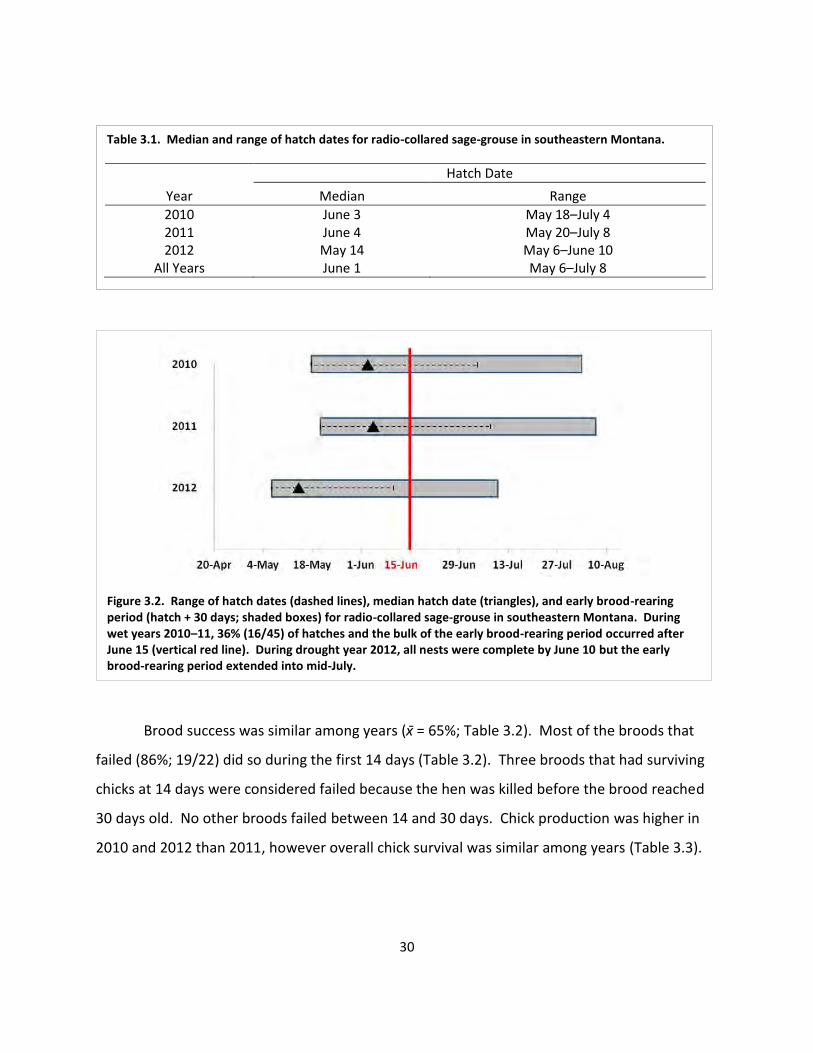
30

Brood success was similar among years ( = 65%; Table 3.2). Most of the broods that

failed (86%; 19/22) did so during the first 14 days (Table 3.2). Three broods that had surviving

chicks at 14 days were considered failed because the hen was killed before the brood reached

30 days old. No other broods failed between 14 and 30 days. Chick production was higher in

2010 and 2012 than 2011, however overall chick survival was similar among years (Table 3.3).

Figure 3.2. Range of hatch dates (dashed lines), median hatch date (triangles), and early brood-rearing period (hatch + 30 days; shaded boxes) for radio-collared sage-grouse in southeastern Montana. During wet years 2010–11, 36% (16/45) of hatches and the bulk of the early brood-rearing period occurred after June 15 (vertical red line). During drought year 2012, all nests were complete by June 10 but the early brood-rearing period extended into mid-July.

Table 3.1. Median and range of hatch dates for radio-collared sage-grouse in southeastern Montana.

Hatch Date

Year Median Range

2010 June 3 May 18–July 4 2011 June 4 May 20–July 8 2012 May 14 May 6–June 10

All Years June 1 May 6–July 8

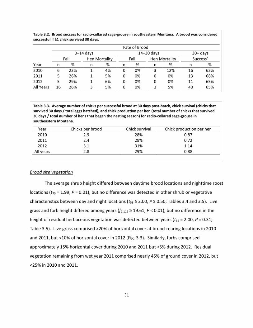
31

Brood site vegetation

The average shrub height differed between daytime brood locations and nighttime roost

locations (t75 = 1.99, P = 0.01), but no difference was detected in other shrub or vegetative

characteristics between day and night locations (t58 ≥ 2.00, P ≥ 0.50; Tables 3.4 and 3.5). Live

grass and forb height differed among years (f2,112 ≥ 19.61, P < 0.01), but no difference in the

height of residual herbaceous vegetation was detected between years (t55 = 2.00, P = 0.31;

Table 3.5). Live grass comprised >20% of horizontal cover at brood-rearing locations in 2010

and 2011, but <10% of horizontal cover in 2012 (Fig. 3.3). Similarly, forbs comprised

approximately 15% horizontal cover during 2010 and 2011 but <5% during 2012. Residual

vegetation remaining from wet year 2011 comprised nearly 45% of ground cover in 2012, but

<25% in 2010 and 2011.

Table 3.3. Average number of chicks per successful brood at 30 days post-hatch, chick survival (chicks that survived 30 days / total eggs hatched), and chick production per hen (total number of chicks that survived 30 days / total number of hens that began the nesting season) for radio-collared sage-grouse in southeastern Montana.

Year Chicks per brood Chick survival Chick production per hen

2010 2.9 28% 0.87 2011 2.4 29% 0.72 2012 3.1 31% 1.14

All years 2.8 29% 0.88

Table 3.2. Brood success for radio-collared sage-grouse in southeastern Montana. A brood was considered successful if ≥1 chick survived 30 days.

Fate of Brood

0–14 days 14–30 days 30+ days Fail Hen Mortality Fail Hen Mortality Successa

Year n % n % n % n % n %

2010 6 23% 1 4% 0 0% 3 12% 16 62% 2011 5 26% 1 5% 0 0% 0 0% 13 68% 2012 5 29% 1 6% 0 0% 0 0% 11 65% All Years 16 26% 3 5% 0 0% 3 5% 40 65%

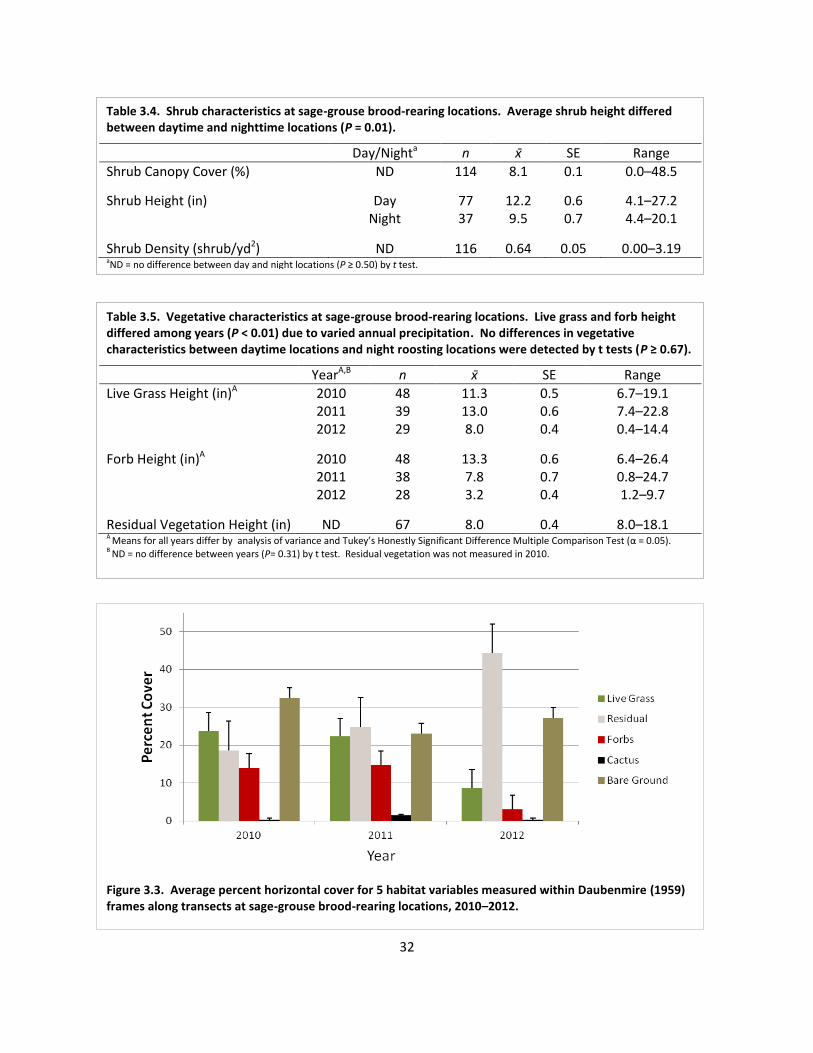
32

Table 3.5. Vegetative characteristics at sage-grouse brood-rearing locations. Live grass and forb height differed among years (P < 0.01) due to varied annual precipitation. No differences in vegetative characteristics between daytime locations and night roosting locations were detected by t tests (P ≥ 0.67).

YearA,B n SE Range

Live Grass Height (in)A 2010 48 11.3 0.5 6.7–19.1 2011 39 13.0 0.6 7.4–22.8 2012 29 8.0 0.4 0.4–14.4

Forb Height (in)A 2010 48 13.3 0.6 6.4–26.4 2011 38 7.8 0.7 0.8–24.7 2012 28 3.2 0.4 1.2–9.7

Residual Vegetation Height (in) ND 67 8.0 0.4 8.0–18.1 A Means for all years differ by analysis of variance and Tukey’s Honestly Significant Difference Multiple Comparison Test (α = 0.05). B ND = no difference between years (P= 0.31) by t test. Residual vegetation was not measured in 2010.

Table 3.4. Shrub characteristics at sage-grouse brood-rearing locations. Average shrub height differed between daytime and nighttime locations (P = 0.01).

Day/Nighta n SE Range

Shrub Canopy Cover (%) ND 114 8.1 0.1 0.0–48.5

Shrub Height (in) Day 77 12.2 0.6 4.1–27.2 Night 37 9.5 0.7 4.4–20.1

Shrub Density (shrub/yd2) ND 116 0.64 0.05 0.00–3.19 aND = no difference between day and night locations (P ≥ 0.50) by t test.

Figure 3.3. Average percent horizontal cover for 5 habitat variables measured within Daubenmire (1959) frames along transects at sage-grouse brood-rearing locations, 2010–2012.

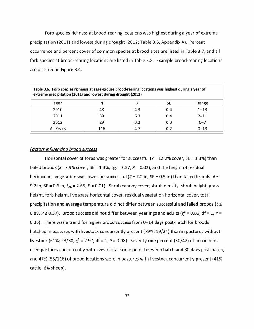
33

Forb species richness at brood-rearing locations was highest during a year of extreme

precipitation (2011) and lowest during drought (2012; Table 3.6, Appendix A). Percent

occurrence and percent cover of common species at brood sites are listed in Table 3.7, and all

forb species at brood-rearing locations are listed in Table 3.8. Example brood-rearing locations

are pictured in Figure 3.4.

Factors influencing brood success

Horizontal cover of forbs was greater for successful ( = 12.2% cover, SE = 1.3%) than

failed broods ( =7.9% cover, SE = 1.3%; t50 = 2.37, P = 0.02), and the height of residual

herbaceous vegetation was lower for successful ( = 7.2 in, SE = 0.5 in) than failed broods ( =

9.2 in, SE = 0.6 in; t26 = 2.65, P = 0.01). Shrub canopy cover, shrub density, shrub height, grass

height, forb height, live grass horizontal cover, residual vegetation horizontal cover, total

precipitation and average temperature did not differ between successful and failed broods (t ≤

0.89, P ≥ 0.37). Brood success did not differ between yearlings and adults (χ² = 0.86, df = 1, P =

0.36). There was a trend for higher brood success from 0–14 days post-hatch for broods

hatched in pastures with livestock concurrently present (79%; 19/24) than in pastures without

livestock (61%; 23/38; χ² = 2.97, df = 1, P = 0.08). Seventy-one percent (30/42) of brood hens

used pastures concurrently with livestock at some point between hatch and 30 days post-hatch,

and 47% (55/116) of brood locations were in pastures with livestock concurrently present (41%

cattle, 6% sheep).

Table 3.6. Forb species richness at sage-grouse brood-rearing locations was highest during a year of extreme precipitation (2011) and lowest during drought (2012).

Year N x SE Range

2010 48 4.3 0.4 1–13

2011 39 6.3 0.4 2–11

2012 29 3.3 0.3 0–7

All Years 116 4.7 0.2 0–13

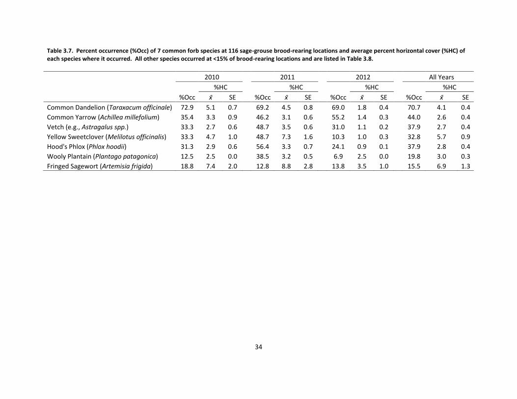
34

Table 3.7. Percent occurrence (%Occ) of 7 common forb species at 116 sage-grouse brood-rearing locations and average percent horizontal cover (%HC) of each species where it occurred. All other species occurred at <15% of brood-rearing locations and are listed in Table 3.8.

2010 2011 2012 All Years

%HC

%HC

%HC

%HC

%Occ SE

%Occ SE

%Occ SE

%Occ SE

Common Dandelion (Taraxacum officinale) 72.9 5.1 0.7

69.2 4.5 0.8

69.0 1.8 0.4

70.7 4.1 0.4

Common Yarrow (Achillea millefolium) 35.4 3.3 0.9

46.2 3.1 0.6

55.2 1.4 0.3

44.0 2.6 0.4

Vetch (e.g., Astragalus spp.) 33.3 2.7 0.6

48.7 3.5 0.6

31.0 1.1 0.2

37.9 2.7 0.4

Yellow Sweetclover (Melilotus officinalis) 33.3 4.7 1.0

48.7 7.3 1.6

10.3 1.0 0.3

32.8 5.7 0.9

Hood's Phlox (Phlox hoodii) 31.3 2.9 0.6

56.4 3.3 0.7

24.1 0.9 0.1

37.9 2.8 0.4

Wooly Plantain (Plantago patagonica) 12.5 2.5 0.0

38.5 3.2 0.5

6.9 2.5 0.0

19.8 3.0 0.3

Fringed Sagewort (Artemisia frigida) 18.8 7.4 2.0

12.8 8.8 2.8

13.8 3.5 1.0

15.5 6.9 1.3

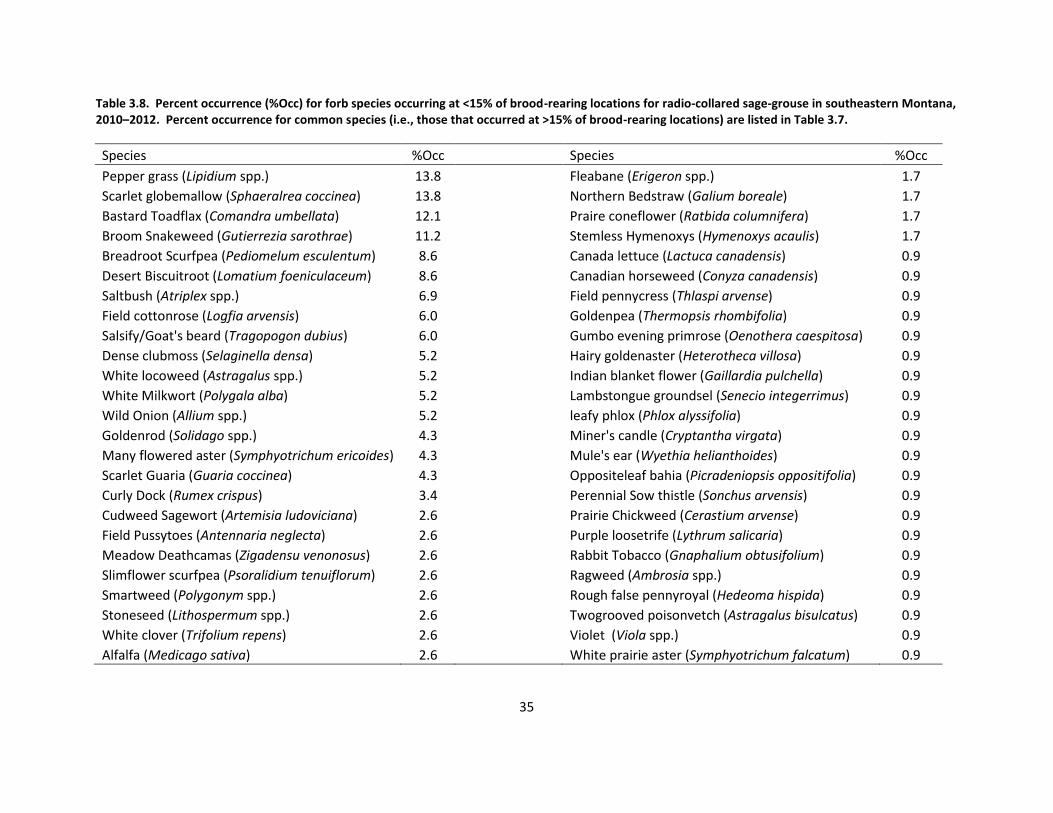
35

Table 3.8. Percent occurrence (%Occ) for forb species occurring at <15% of brood-rearing locations for radio-collared sage-grouse in southeastern Montana, 2010–2012. Percent occurrence for common species (i.e., those that occurred at >15% of brood-rearing locations) are listed in Table 3.7.

Species %Occ

Species %Occ

Pepper grass (Lipidium spp.) 13.8

Fleabane (Erigeron spp.) 1.7

Scarlet globemallow (Sphaeralrea coccinea) 13.8

Northern Bedstraw (Galium boreale) 1.7

Bastard Toadflax (Comandra umbellata) 12.1

Praire coneflower (Ratbida columnifera) 1.7

Broom Snakeweed (Gutierrezia sarothrae) 11.2

Stemless Hymenoxys (Hymenoxys acaulis) 1.7

Breadroot Scurfpea (Pediomelum esculentum) 8.6

Canada lettuce (Lactuca canadensis) 0.9

Desert Biscuitroot (Lomatium foeniculaceum) 8.6

Canadian horseweed (Conyza canadensis) 0.9

Saltbush (Atriplex spp.) 6.9

Field pennycress (Thlaspi arvense) 0.9

Field cottonrose (Logfia arvensis) 6.0

Goldenpea (Thermopsis rhombifolia) 0.9

Salsify/Goat's beard (Tragopogon dubius) 6.0

Gumbo evening primrose (Oenothera caespitosa) 0.9

Dense clubmoss (Selaginella densa) 5.2

Hairy goldenaster (Heterotheca villosa) 0.9

White locoweed (Astragalus spp.) 5.2

Indian blanket flower (Gaillardia pulchella) 0.9

White Milkwort (Polygala alba) 5.2

Lambstongue groundsel (Senecio integerrimus) 0.9

Wild Onion (Allium spp.) 5.2

leafy phlox (Phlox alyssifolia) 0.9

Goldenrod (Solidago spp.) 4.3

Miner's candle (Cryptantha virgata) 0.9

Many flowered aster (Symphyotrichum ericoides) 4.3

Mule's ear (Wyethia helianthoides) 0.9

Scarlet Guaria (Guaria coccinea) 4.3

Oppositeleaf bahia (Picradeniopsis oppositifolia) 0.9

Curly Dock (Rumex crispus) 3.4

Perennial Sow thistle (Sonchus arvensis) 0.9

Cudweed Sagewort (Artemisia ludoviciana) 2.6

Prairie Chickweed (Cerastium arvense) 0.9

Field Pussytoes (Antennaria neglecta) 2.6

Purple loosetrife (Lythrum salicaria) 0.9

Meadow Deathcamas (Zigadensu venonosus) 2.6

Rabbit Tobacco (Gnaphalium obtusifolium) 0.9

Slimflower scurfpea (Psoralidium tenuiflorum) 2.6

Ragweed (Ambrosia spp.) 0.9

Smartweed (Polygonym spp.) 2.6

Rough false pennyroyal (Hedeoma hispida) 0.9

Stoneseed (Lithospermum spp.) 2.6

Twogrooved poisonvetch (Astragalus bisulcatus) 0.9

White clover (Trifolium repens) 2.6

Violet (Viola spp.) 0.9

Alfalfa (Medicago sativa) 2.6

White prairie aster (Symphyotrichum falcatum) 0.9

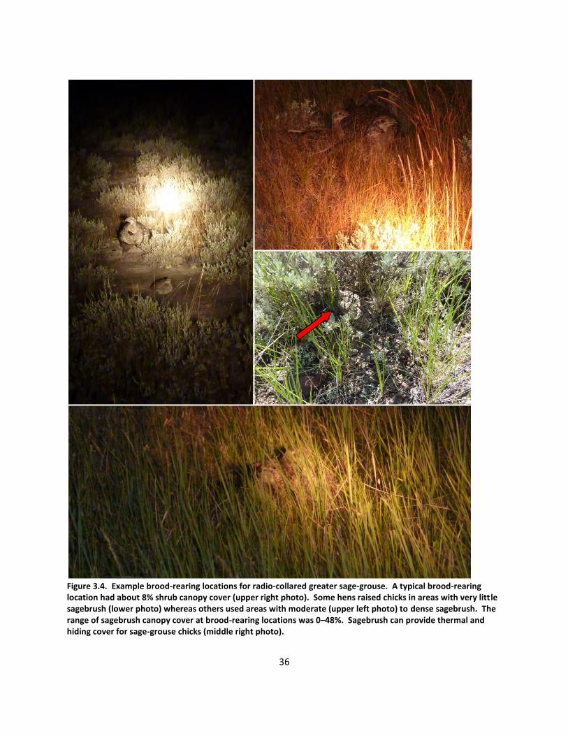
36

Figure 3.4. Example brood-rearing locations for radio-collared greater sage-grouse. A typical brood-rearing location had about 8% shrub canopy cover (upper right photo). Some hens raised chicks in areas with very little sagebrush (lower photo) whereas others used areas with moderate (upper left photo) to dense sagebrush. The range of sagebrush canopy cover at brood-rearing locations was 0–48%. Sagebrush can provide thermal and hiding cover for sage-grouse chicks (middle right photo).

37

DISCUSSION

Wet conditions during 2010 and 2011 resulted in a protracted nesting season, with 36%

of hatches and the bulk of the early brood-rearing period occurring after June 15. Nesting

season 2010 occurred during a drought year following a mild winter (Appendix A), and all nests

hatched by June 15 but the early brood-rearing period extended to July 10. Therefore, timing

restrictions that end on June 15 will not benefit later nesting hens or young broods in most

years. Timing of hatch and the early brood-rearing period during a “normal” year might be

expected to be intermediate between wet years 2010 and 2011 and drought year 2012, with a

median hatch date of approximately May 24 and latest hatch date of June 24. If timing

restrictions were maintained until July 15, it would be reasonable to assume that in most years

nearly all nesting would be complete, nearly all chicks would be >2 weeks old, and more than

half of broods would have reached 30 days. Extending timing restrictions to benefit young

sage-grouse chicks may be important because most chick mortality occurs within the first 4

weeks after hatching (Gregg et al. 2007, Dahlgren et al. 2010a), and chick survival is one of the

most important parameters influencing population growth rates for sage-grouse (Taylor et al.

2010). However, timing restrictions are only effective for minimally invasive, short duration

projects and cannot be expected to offset the impacts of long-term habitat loss, fragmentation,

or degradation.

Of 62 broods, 40 (65%) had chicks survive to 30 days. One brood hen mortality occurred

between hatching and 14 days in each of the 3 years, and 3 brood hens died between 14 and 30

days post-hatch in 2010. Sage-grouse hens commonly mix broods and adopt orphans (Dahlgren

et al. 2010a), and consequently it is possible that some orphaned chicks in our study survived.

Survival of orphaned chicks that are less than 10 days old is probably low due to the solitary

nature of hens with young chicks (Dalke et al. 1963), but survival of broods over 10 days old

may approach 100% because hen locations tend to overlap as chicks grow, and older chicks

may survive several days without a brood hen before being adopted (Patterson 1952, Keppie

1977, Connelly et al. 2006). Further, spotlight counts are highly accurate but it is possible that

detection was <100% during nighttime brood counts (Dahlgren et al. 2010b). Thus, reported

values for brood success and chick production are minimum estimates.

38

Comparison of brood and chick survival among studies is confounded because

researchers have used different field methods and intervals (ranging from 18–51 days post-

hatch) to quantify brood and chick survival (reviewed in Connelly et al. 2011a). However, it

may be reasonable to compare estimates for brood and chick survival for different durations

post-hatch given that chick mortality is highest immediately post-hatch and survival is expected

to be high during the period of discrepancy (Sika 2006, Gregg et al. 2007). Our estimate of 65%

for brood survival is in the middle of the range reported by other researchers (21–100%;

reviewed in Sika 2006). It was above the range reported from northwestern South Dakota (32–

52%; Kaczor 2008) and southwestern North Dakota (34–42%; Herman-Brunson 2007), at the

high end of the range reported for northcentral Montana (21–76%; Moynahan 2004), and

below the range reported from central Montana (71–84%; Sika 2006). Similarly, our estimate

for chick survival (29%) is in the middle of the range reported by other researchers (12–50%;

reviewed in Connelly et al. 2011a).

Brood and chick survival vary among years and study areas (Connelly et al. 2011a) but

were remarkably consistent between very wet and very dry years in our study (Tables 3.2 and

3.3, Appendix A). Cold, wet weather may be devastating to young chicks because they cannot

thermoregulate independently (Patterson 1952, Wallestad 1975), thus we expected brood and

chick survival would be related to weather variables and lower in 2010 and 2011 than 2012.

However, when food is abundant chicks do not need to spend as much time and effort foraging

and may avoid exposure by spending considerable time brooding during cold, rainy days

(Zwickel 1967, Connelly et al. 2006). Abundant forbs and insects (especially grasshoppers;

based on field observation) provided ample forage for chicks during wet years 2010 and 2011,

and may have helped chicks survive in the face of harsh weather conditions. Conversely,

weather for broods was favorable in 2012, but drought conditions resulted in low forb

abundance and concomitantly insect abundance (Southwood and Cross 2002) which can limit

brood survival (Peterson 1970, Drut et al. 1994b). Adequate cover (live vegetation in 2010 and

2011 and residual vegetation in 2012; Fig. 3.3) was available to broods during all years of the

study, and may have contributed to similar rates of brood and chick survival among years.

39

Unlike brood and chick survival, chick production varied among years. Chick production

is influenced by a variety of reproductive parameters including hen survival, nest success, hatch

rates, and chick survival, and therefore represents a comprehensive measure of sage-grouse

annual production. Chick production was lowest in 2011, which resulted from extreme

moisture during that year (Appendix A) that caused lower nest success, reduced hatch rates (Fig

2.1), and therefore a lower average number of chicks per brood.

Brood-rearing sage-grouse tended to use open stands of sagebrush ( = 8% canopy

cover), which is similar to studies elsewhere (e.g., Wallestad 1971, Connelly 1982). Brood

success during the first 14 days post-hatch was not related to shrub characteristics, which

suggests that adequate shrub cover was available for broods, or that shrub cover is secondary

to other habitat features (e.g., forb availability) for brood survival. Shrub canopy cover and

density were similar between day and night locations, but the average shrub height was slightly

higher at daytime brood locations than nighttime roost locations. We suspect that slightly

taller shrubs may offer better cover from avian predators during daylight hours.

Grass cover at brood-rearing sites was related to annual precipitation ( height: 8–13 in),

but was not related to brood success. Researchers elsewhere have reported conflicting results,

probably an artifact of location, soil type, grass composition, and grass availability. Some

suggest that brood hens select areas with taller grass than random locations (e.g., = 16.7 in,

Aldridge and Brigham 2002), whereas others have reported that brood hens select areas with

short grass (e.g., < 7 in, Sveum et al. 1998). Live and residual vegetation can provide valuable

cover from predators but cover that is too dense can inhibit brood hens from detecting and

escaping predators (Aldridge 2005, Gregg and Crawford 2009), and can also contribute to

exposure-related death of chicks during cold, wet days (Patterson 1952), which may explain our

counterintuitive finding that residual vegetation was shorter for successful broods. Optimal

grass cover given these opposing effects is probably related to individual site characteristics,

weather during the brood-rearing period, and the structure and composition of other

vegetative components. Grass cover did not differ between successful and failed broods, which

suggests grass cover was secondary to other habitat features (i.e., forbs).

40

Forbs comprised approximately 15% horizontal cover at brood sites during 2010 and

2011 but less than 5% during drought year 2012, and forb cover was higher for successful

(12.2% cover) than failed (7.9% cover) broods. Sage-grouse researchers elsewhere have

reported similar (7–14%) forb cover during early brood-rearing and the importance of forbs for

chick survival (e.g., Schoenberg 1982, Drut et al. 1994a,b, Aldridge and Brigham 2002). As

upland vegetation desiccates and senesces, brood hens tend to move to mesic areas with high

(up to 41%) forb cover to meet the dietary requirements of chicks (e.g., Peterson 1970, Dunn

and Braun 1986, Sveum et al. 1998). We did not quantify vegetation use during late brood-

rearing due to logistic constraints, but we did observe a trend toward grouse using more mesic

areas during late brood-rearing. Forty percent of locations were within 100 yards of a creek,

pond, or wetland for late brood-rearing hens compared to 25% for broodless hens and 16% for

early brood-rearing hens (see Chapter 6).

Similar to forb cover, forb species richness at brood-rearing locations was highest during

a year of extreme precipitation (2011) and lowest during drought (2012; Table 3.6). Percent

occurrence and cover of common species were fairly consistent among years (Table 3.7). We

did not quantify forb availability at random sites. However, 2011 was a sweet clover “boom”

year, and sweet clover was the dominant species in many parts of the study area (field

observation, Fig. 3.5). Sweet clover was present at 49% of brood-rearing locations but only

comprised an average 7% and maximum 16% cover where it occurred, indicating that areas of

dense sweet clover were not preferred brood-rearing habitat (Fig. 3.5, Table 3.7).

Brood success was higher in pastures with livestock concurrently present (79%) than in

pastures without livestock (61%). The mechanism for this is unknown; it may be a result of

behavioral avoidance of livestock by predators (Kirby and Grosz 1995), or predator control

efforts in areas with livestock. Extensive use of pastures concurrent with livestock is a strong

indicator that brood hens did not avoid livestock, but nor did they exhibit strong selection for

pastures with livestock. Over 70% of brood hens used pastures with livestock at some point

during the first 30 days post-hatch (a rough idea of availability), but only 47% of brood-rearing

locations were in pastures with livestock. Hens are probably selecting areas based on forage

and cover for broods rather than simply livestock presence. Recently grazed pastures may be

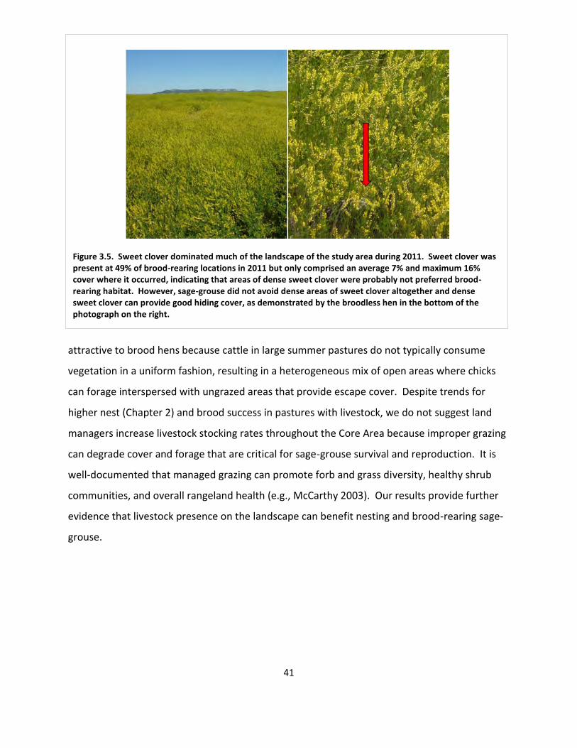
41

Figure 3.5. Sweet clover dominated much of the landscape of the study area during 2011. Sweet clover was present at 49% of brood-rearing locations in 2011 but only comprised an average 7% and maximum 16% cover where it occurred, indicating that areas of dense sweet clover were probably not preferred brood-rearing habitat. However, sage-grouse did not avoid dense areas of sweet clover altogether and dense sweet clover can provide good hiding cover, as demonstrated by the broodless hen in the bottom of the photograph on the right.

attractive to brood hens because cattle in large summer pastures do not typically consume

vegetation in a uniform fashion, resulting in a heterogeneous mix of open areas where chicks

can forage interspersed with ungrazed areas that provide escape cover. Despite trends for

higher nest (Chapter 2) and brood success in pastures with livestock, we do not suggest land

managers increase livestock stocking rates throughout the Core Area because improper grazing

can degrade cover and forage that are critical for sage-grouse survival and reproduction. It is

well-documented that managed grazing can promote forb and grass diversity, healthy shrub

communities, and overall rangeland health (e.g., McCarthy 2003). Our results provide further

evidence that livestock presence on the landscape can benefit nesting and brood-rearing sage-

grouse.

- 4 -

Hen Survival

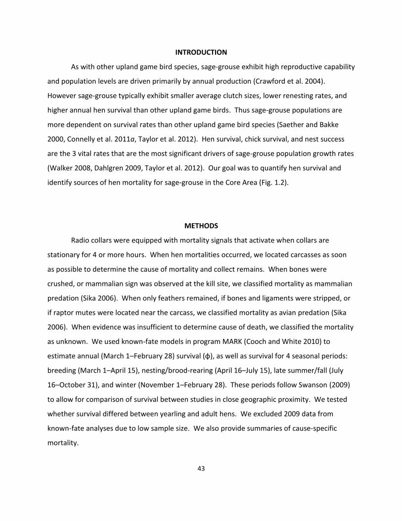
43

INTRODUCTION

As with other upland game bird species, sage-grouse exhibit high reproductive capability

and population levels are driven primarily by annual production (Crawford et al. 2004).

However sage-grouse typically exhibit smaller average clutch sizes, lower renesting rates, and

higher annual hen survival than other upland game birds. Thus sage-grouse populations are

more dependent on survival rates than other upland game bird species (Saether and Bakke

2000, Connelly et al. 2011a, Taylor et al. 2012). Hen survival, chick survival, and nest success

are the 3 vital rates that are the most significant drivers of sage-grouse population growth rates

(Walker 2008, Dahlgren 2009, Taylor et al. 2012). Our goal was to quantify hen survival and

identify sources of hen mortality for sage-grouse in the Core Area (Fig. 1.2).

METHODS

Radio collars were equipped with mortality signals that activate when collars are

stationary for 4 or more hours. When hen mortalities occurred, we located carcasses as soon

as possible to determine the cause of mortality and collect remains. When bones were

crushed, or mammalian sign was observed at the kill site, we classified mortality as mammalian

predation (Sika 2006). When only feathers remained, if bones and ligaments were stripped, or

if raptor mutes were located near the carcass, we classified mortality as avian predation (Sika

2006). When evidence was insufficient to determine cause of death, we classified the mortality

as unknown. We used known-fate models in program MARK (Cooch and White 2010) to

estimate annual (March 1–February 28) survival (φ), as well as survival for 4 seasonal periods:

breeding (March 1–April 15), nesting/brood-rearing (April 16–July 15), late summer/fall (July

16–October 31), and winter (November 1–February 28). These periods follow Swanson (2009)

to allow for comparison of survival between studies in close geographic proximity. We tested

whether survival differed between yearling and adult hens. We excluded 2009 data from

known-fate analyses due to low sample size. We also provide summaries of cause-specific

mortality.

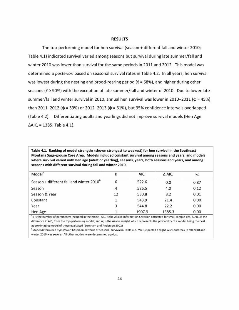
44

RESULTS

The top-performing model for hen survival (season + different fall and winter 2010;

Table 4.1) indicated survival varied among seasons but survival during late summer/fall and

winter 2010 was lower than survival for the same periods in 2011 and 2012. This model was

determined a posteriori based on seasonal survival rates in Table 4.2. In all years, hen survival

was lowest during the nesting and brood-rearing period ( = 68%), and higher during other

seasons ( ≥ 90%) with the exception of late summer/fall and winter of 2010. Due to lower late

summer/fall and winter survival in 2010, annual hen survival was lower in 2010–2011 (φ = 45%)

than 2011–2012 (φ = 59%) or 2012–2013 (φ = 61%), but 95% confidence intervals overlapped

(Table 4.2). Differentiating adults and yearlings did not improve survival models (Hen Age

ΔAICc = 1385; Table 4.1).

Table 4.1. Ranking of model strengths (shown strongest to weakest) for hen survival in the Southeast Montana Sage-grouse Core Area. Models included constant survival among seasons and years, and models where survival varied with hen age (adult or yearling), seasons, years, both seasons and years, and among seasons with different survival during fall and winter 2010.

ModelA K AICc Δ AICc wi

Season + different fall and winter 2010B 6 522.6 0.0 0.87

Season 4 526.5 4.0 0.12

Season & Year 12 530.8 8.2 0.01

Constant 1 543.9 21.4 0.00

Year 3 544.8 22.2 0.00

Hen Age 1 1907.9 1385.3 0.00 AK is the number of parameters included in the model, AICc is the Akaike Information Criterion corrected for small sample size, Δ AICc is the

difference in AICc from the top-performing model, and wi is the Akaike weight which represents the probability of a model being the best

approximating model of those evaluated (Burnham and Anderson 2002) BModel determined a posteriori based on patterns of seasonal survival in Table 4.2. We suspected a slight WNv outbreak in fall 2010 and

winter 2010 was severe. All other models were determined a priori.

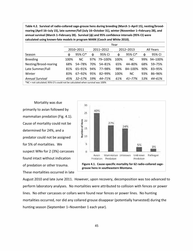
45

Figure 4.1. Cause-specific mortality for 62 radio-collared sage-grouse hens in southeastern Montana.

Mortality was due

primarily to avian followed by

mammalian predation (Fig. 4.1).

Cause of mortality could not be

determined for 24%, and a

predator could not be assigned

for 5% of mortalities. We

suspect WNv for 2 (3%) carcasses

found intact without indication

of predation or other trauma.

These mortalities occurred in late

August 2010 and late June 2011. However, upon recovery, decomposition was too advanced to

perform laboratory analyses. No mortalities were attributed to collision with fences or power

lines. No other carcasses or collars were found near fences or power lines. No hunting

mortalities occurred, nor did any collared grouse disappear (potentially harvested) during the

hunting season (September 1–November 1 each year).

Table 4.2. Survival of radio-collared sage-grouse hens during breeding (March 1–April 15), nesting/brood-

rearing (April 16–July 15), late summer/fall (July 16–October 31), winter (November 1–February 28), and

annual survival (March 1–February 28). Survival (φ) and 95% confidence intervals (95% CI) were

calculated using known-fate models in program MARK (Cooch and White 2010).

Year

2010–2011

2011–2012

2012–2013

All Years

Season φ 95% CI* φ 95% CI

φ 95% CI*

φ 95% CI

Breeding 100% NC 97% 79–100%

100% NC

99% 94–100%

Nesting/Brood-rearing 68% 54–78% 70% 54–81%

65% 44–80%

68% 59–75%

Late Summer/Fall 81% 65–91% 94% 77–98%

98% 84–100%

90% 83–95%

Winter 83% 67–92% 95% 82–99%

100% NC

93% 86–96%

Annual Survival 45% 32–57% 59% 44–71%

61% 41–77%

53% 44–61%

*NC = not calculated; 95% CI’s could not be calculated when survival was 100%

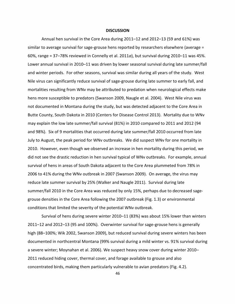
46

DISCUSSION

Annual hen survival in the Core Area during 2011–12 and 2012–13 (59 and 61%) was

similar to average survival for sage-grouse hens reported by researchers elsewhere (average =

60%, range = 37–78% reviewed in Connelly et al. 2011a), but survival during 2010–11 was 45%.

Lower annual survival in 2010–11 was driven by lower seasonal survival during late summer/fall

and winter periods. For other seasons, survival was similar during all years of the study. West

Nile virus can significantly reduce survival of sage-grouse during late summer to early fall, and

mortalities resulting from WNv may be attributed to predation when neurological effects make

hens more susceptible to predators (Swanson 2009, Naugle et al. 2004). West Nile virus was

not documented in Montana during the study, but was detected adjacent to the Core Area in

Butte County, South Dakota in 2010 (Centers for Disease Control 2013). Mortality due to WNv

may explain the low late summer/fall survival (81%) in 2010 compared to 2011 and 2012 (94

and 98%). Six of 9 mortalities that occurred during late summer/fall 2010 occurred from late

July to August, the peak period for WNv outbreaks. We did suspect WNv for one mortality in

2010. However, even though we observed an increase in hen mortality during this period, we

did not see the drastic reduction in hen survival typical of WNv outbreaks. For example, annual

survival of hens in areas of South Dakota adjacent to the Core Area plummeted from 78% in

2006 to 41% during the WNv outbreak in 2007 (Swanson 2009). On average, the virus may

reduce late summer survival by 25% (Walker and Naugle 2011). Survival during late

summer/fall 2010 in the Core Area was reduced by only 15%, perhaps due to decreased sage-

grouse densities in the Core Area following the 2007 outbreak (Fig. 1.3) or environmental

conditions that limited the severity of the potential WNv outbreak.

Survival of hens during severe winter 2010–11 (83%) was about 15% lower than winters

2011–12 and 2012–13 (95 and 100%). Overwinter survival for sage-grouse hens is generally

high (88–100%; Wik 2002, Swanson 2009), but reduced survival during severe winters has been

documented in northcentral Montana (99% survival during a mild winter vs. 91% survival during

a severe winter; Moynahan et al. 2006). We suspect heavy snow cover during winter 2010–

2011 reduced hiding cover, thermal cover, and forage available to grouse and also

concentrated birds, making them particularly vulnerable to avian predators (Fig. 4.2).

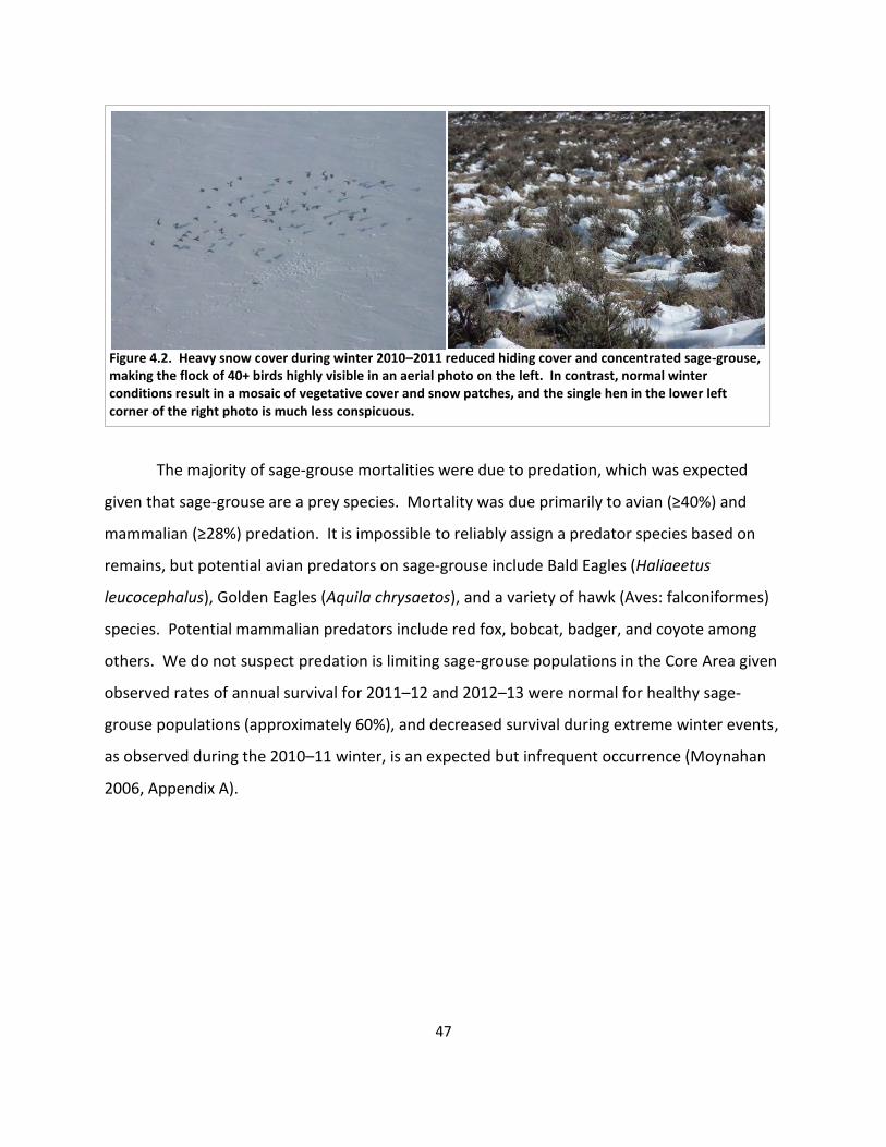
47

The majority of sage-grouse mortalities were due to predation, which was expected

given that sage-grouse are a prey species. Mortality was due primarily to avian (≥40%) and

mammalian (≥28%) predation. It is impossible to reliably assign a predator species based on

remains, but potential avian predators on sage-grouse include Bald Eagles (Haliaeetus

leucocephalus), Golden Eagles (Aquila chrysaetos), and a variety of hawk (Aves: falconiformes)

species. Potential mammalian predators include red fox, bobcat, badger, and coyote among

others. We do not suspect predation is limiting sage-grouse populations in the Core Area given

observed rates of annual survival for 2011–12 and 2012–13 were normal for healthy sage-

grouse populations (approximately 60%), and decreased survival during extreme winter events,

as observed during the 2010–11 winter, is an expected but infrequent occurrence (Moynahan

2006, Appendix A).

Figure 4.2. Heavy snow cover during winter 2010–2011 reduced hiding cover and concentrated sage-grouse, making the flock of 40+ birds highly visible in an aerial photo on the left. In contrast, normal winter conditions result in a mosaic of vegetative cover and snow patches, and the single hen in the lower left corner of the right photo is much less conspicuous.

- 5 -

Population Viability

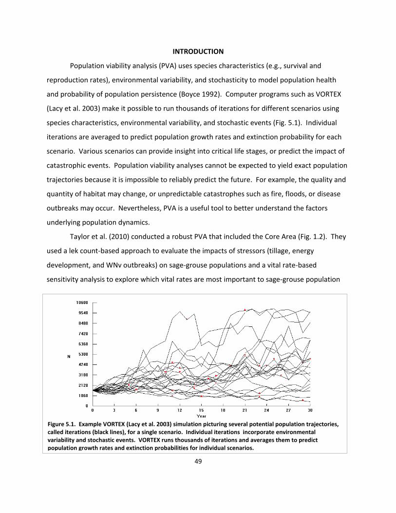
49

INTRODUCTION

Population viability analysis (PVA) uses species characteristics (e.g., survival and

reproduction rates), environmental variability, and stochasticity to model population health

and probability of population persistence (Boyce 1992). Computer programs such as VORTEX

(Lacy et al. 2003) make it possible to run thousands of iterations for different scenarios using

species characteristics, environmental variability, and stochastic events (Fig. 5.1). Individual

iterations are averaged to predict population growth rates and extinction probability for each

scenario. Various scenarios can provide insight into critical life stages, or predict the impact of

catastrophic events. Population viability analyses cannot be expected to yield exact population

trajectories because it is impossible to reliably predict the future. For example, the quality and

quantity of habitat may change, or unpredictable catastrophes such as fire, floods, or disease

outbreaks may occur. Nevertheless, PVA is a useful tool to better understand the factors

underlying population dynamics.

Taylor et al. (2010) conducted a robust PVA that included the Core Area (Fig. 1.2). They

used a lek count-based approach to evaluate the impacts of stressors (tillage, energy

development, and WNv outbreaks) on sage-grouse populations and a vital rate-based

sensitivity analysis to explore which vital rates are most important to sage-grouse population

Figure 5.1. Example VORTEX (Lacy et al. 2003) simulation picturing several potential population trajectories, called iterations (black lines), for a single scenario. Individual iterations incorporate environmental variability and stochastic events. VORTEX runs thousands of iterations and averages them to predict population growth rates and extinction probabilities for individual scenarios.

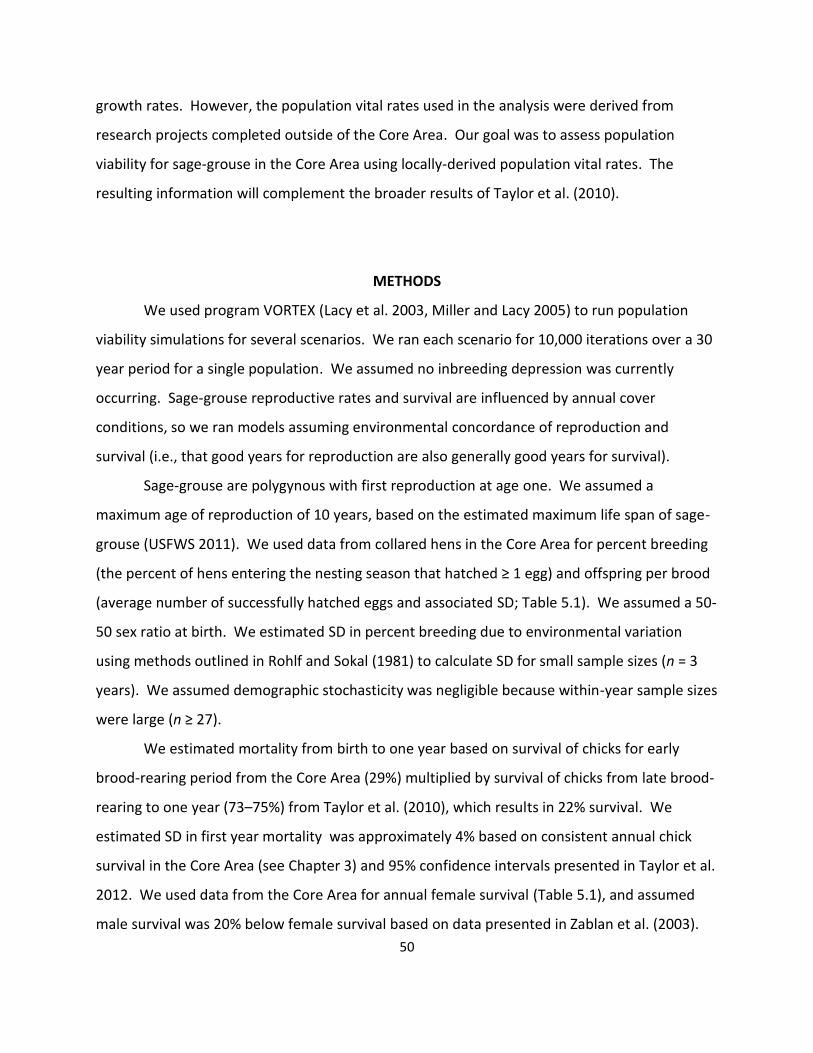
50

growth rates. However, the population vital rates used in the analysis were derived from

research projects completed outside of the Core Area. Our goal was to assess population

viability for sage-grouse in the Core Area using locally-derived population vital rates. The

resulting information will complement the broader results of Taylor et al. (2010).

METHODS

We used program VORTEX (Lacy et al. 2003, Miller and Lacy 2005) to run population

viability simulations for several scenarios. We ran each scenario for 10,000 iterations over a 30

year period for a single population. We assumed no inbreeding depression was currently

occurring. Sage-grouse reproductive rates and survival are influenced by annual cover

conditions, so we ran models assuming environmental concordance of reproduction and

survival (i.e., that good years for reproduction are also generally good years for survival).

Sage-grouse are polygynous with first reproduction at age one. We assumed a

maximum age of reproduction of 10 years, based on the estimated maximum life span of sage-

grouse (USFWS 2011). We used data from collared hens in the Core Area for percent breeding

(the percent of hens entering the nesting season that hatched ≥ 1 egg) and offspring per brood

(average number of successfully hatched eggs and associated SD; Table 5.1). We assumed a 50-

50 sex ratio at birth. We estimated SD in percent breeding due to environmental variation

using methods outlined in Rohlf and Sokal (1981) to calculate SD for small sample sizes (n = 3

years). We assumed demographic stochasticity was negligible because within-year sample sizes

were large (n ≥ 27).

We estimated mortality from birth to one year based on survival of chicks for early

brood-rearing period from the Core Area (29%) multiplied by survival of chicks from late brood-

rearing to one year (73–75%) from Taylor et al. (2010), which results in 22% survival. We

estimated SD in first year mortality was approximately 4% based on consistent annual chick

survival in the Core Area (see Chapter 3) and 95% confidence intervals presented in Taylor et al.

2012. We used data from the Core Area for annual female survival (Table 5.1), and assumed

male survival was 20% below female survival based on data presented in Zablan et al. (2003).

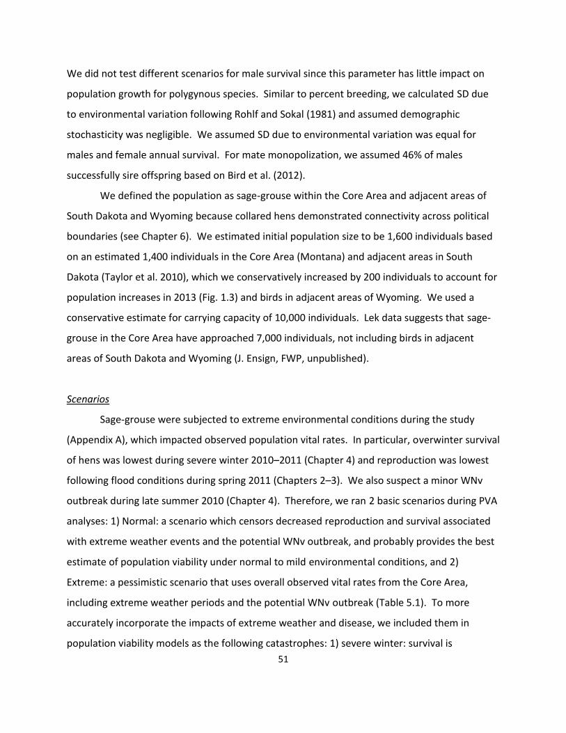
51

We did not test different scenarios for male survival since this parameter has little impact on

population growth for polygynous species. Similar to percent breeding, we calculated SD due

to environmental variation following Rohlf and Sokal (1981) and assumed demographic

stochasticity was negligible. We assumed SD due to environmental variation was equal for

males and female annual survival. For mate monopolization, we assumed 46% of males

successfully sire offspring based on Bird et al. (2012).

We defined the population as sage-grouse within the Core Area and adjacent areas of

South Dakota and Wyoming because collared hens demonstrated connectivity across political

boundaries (see Chapter 6). We estimated initial population size to be 1,600 individuals based

on an estimated 1,400 individuals in the Core Area (Montana) and adjacent areas in South

Dakota (Taylor et al. 2010), which we conservatively increased by 200 individuals to account for

population increases in 2013 (Fig. 1.3) and birds in adjacent areas of Wyoming. We used a

conservative estimate for carrying capacity of 10,000 individuals. Lek data suggests that sage-

grouse in the Core Area have approached 7,000 individuals, not including birds in adjacent

areas of South Dakota and Wyoming (J. Ensign, FWP, unpublished).

Scenarios

Sage-grouse were subjected to extreme environmental conditions during the study

(Appendix A), which impacted observed population vital rates. In particular, overwinter survival

of hens was lowest during severe winter 2010–2011 (Chapter 4) and reproduction was lowest

following flood conditions during spring 2011 (Chapters 2–3). We also suspect a minor WNv

outbreak during late summer 2010 (Chapter 4). Therefore, we ran 2 basic scenarios during PVA

analyses: 1) Normal: a scenario which censors decreased reproduction and survival associated

with extreme weather events and the potential WNv outbreak, and probably provides the best

estimate of population viability under normal to mild environmental conditions, and 2)

Extreme: a pessimistic scenario that uses overall observed vital rates from the Core Area,

including extreme weather periods and the potential WNv outbreak (Table 5.1). To more

accurately incorporate the impacts of extreme weather and disease, we included them in

population viability models as the following catastrophes: 1) severe winter: survival is

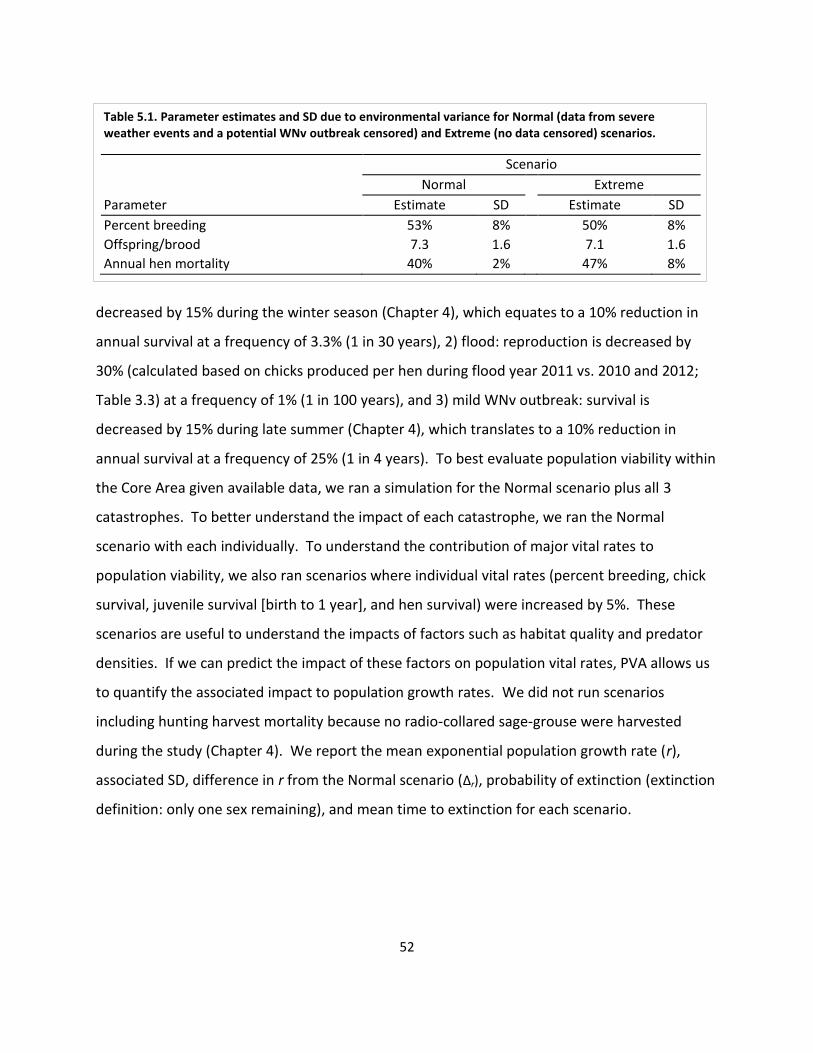
52

Table 5.1. Parameter estimates and SD due to environmental variance for Normal (data from severe weather events and a potential WNv outbreak censored) and Extreme (no data censored) scenarios.

Scenario

Normal Extreme

Parameter Estimate SD Estimate SD

Percent breeding 53% 8% 50% 8%

Offspring/brood 7.3 1.6 7.1 1.6

Annual hen mortality 40% 2% 47% 8%

decreased by 15% during the winter season (Chapter 4), which equates to a 10% reduction in

annual survival at a frequency of 3.3% (1 in 30 years), 2) flood: reproduction is decreased by

30% (calculated based on chicks produced per hen during flood year 2011 vs. 2010 and 2012;

Table 3.3) at a frequency of 1% (1 in 100 years), and 3) mild WNv outbreak: survival is

decreased by 15% during late summer (Chapter 4), which translates to a 10% reduction in

annual survival at a frequency of 25% (1 in 4 years). To best evaluate population viability within

the Core Area given available data, we ran a simulation for the Normal scenario plus all 3

catastrophes. To better understand the impact of each catastrophe, we ran the Normal

scenario with each individually. To understand the contribution of major vital rates to

population viability, we also ran scenarios where individual vital rates (percent breeding, chick

survival, juvenile survival [birth to 1 year], and hen survival) were increased by 5%. These

scenarios are useful to understand the impacts of factors such as habitat quality and predator

densities. If we can predict the impact of these factors on population vital rates, PVA allows us

to quantify the associated impact to population growth rates. We did not run scenarios

including hunting harvest mortality because no radio-collared sage-grouse were harvested

during the study (Chapter 4). We report the mean exponential population growth rate (r),

associated SD, difference in r from the Normal scenario (Δr), probability of extinction (extinction

definition: only one sex remaining), and mean time to extinction for each scenario.

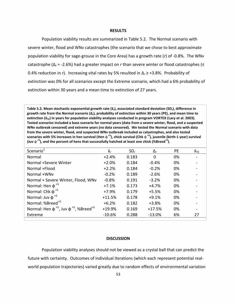
53

Table 5.2. Mean stochastic exponential growth rate ( r), associated standard deviation (SDr), difference in growth rate from the Normal scenario (Δr), probability of extinction within 30 years (PE), and mean time to extinction ( TE) in years for population viability analyses conducted in program VORTEX (Lacy et al. 2003). Tested scenarios included a base scenario for normal years (data from a severe winter, flood, and a suspected WNv outbreak censored) and extreme years (no data censored). We tested the Normal scenario with data from the severe winter, flood, and suspected WNv outbreak included as catastrophes, and also tested scenarios with 5% increases in hen survival (Hen φ

+5), chick survival (Chk φ

+5), juvenile (birth-1 year) survival

(Juv φ +5

), and the percent of hens that successfully hatched at least one chick (%Breed+5

).

Scenario1 x r SDr Δr PE x TE

Normal +2.4% 0.183 0 0% - Normal +Severe Winter +2.0% 0.184 -0.4% 0% -

Normal +Flood +2.2% 0.184 -0.2% 0% - Normal +WNv -0.2% 0.189 -2.6% 0% - Normal + Severe Winter, Flood, WNv -0.8% 0.191 -3.2% 0% - Normal: Hen φ +5 +7.1% 0.173 +4.7% 0% - Normal: Chk φ +5 +7.9% 0.179 +5.5% 0% - Normal: Juv φ +5 +11.5% 0.178 +9.1% 0% - Normal: %Breed+5 +6.2% 0.182 +3.8% 0% - Normal: Hen φ +5, Juv φ +5, %Breed+5 +19.9% 0.169 +17.5% 0% - Extreme -10.6% 0.288 -13.0% 6% 27

RESULTS

Population viability results are summarized in Table 5.2. The Normal scenario with

severe winter, flood and WNv catastrophes (the scenario that we chose to best approximate

population viability for sage-grouse in the Core Area) has a growth rate (r) of -0.8%. The WNv

catastrophe (Δr = -2.6%) had a greater impact on r than severe winter or flood catastrophes (≤

0.4% reduction in r). Increasing vital rates by 5% resulted in Δr ≥ +3.8%. Probability of

extinction was 0% for all scenarios except the Extreme scenario, which had a 6% probability of

extinction within 30 years and a mean time to extinction of 27 years.

DISCUSSION

Population viability analyses should not be viewed as a crystal ball that can predict the

future with certainty. Outcomes of individual iterations (which each represent potential real-

world population trajectories) varied greatly due to random effects of environmental variation

54

and stochasticity. We also caution that data used to conduct this PVA was collected during a

series of extreme years, which impacted rates of survival and reproduction. The Extreme

scenario is certainly pessimistic because it considers data collected during extreme weather

events as common occurrence. However, even though we incorporated observed effects of

extreme weather into the Normal scenario as catastrophes, there were likely other, more

indirect effects of abnormal weather that were impossible to quantify or censor. Therefore,

vital rates used in the Normal scenario may be pessimistic (e.g., due to drought in 2012) or

optimistic (e.g., because cover was good during all years of the study). Although PVA cannot

predict the future with great certainty, it is a useful tool to better understand the likelihood of

population persistence and factors driving population dynamics.

Overall PVA indicates that Core Area sage-grouse are very likely to persist at sustainable

levels. The mean population growth rate for our most realistic scenario (Normal + Severe

Winter, Flood, WNv; r = -0.8%) is indicative of an effectively stable population. Probability of

extinction within 30 years was 0% for nearly every scenario. Even the pessimistic Extreme

scenario had only a 6% probability of extinction in 30 years, and the mean time to extinction

was 27 years. This indicates that even if Core Area populations were to decline as predicted by

the Extreme scenario, local extinction is unlikely to be imminent. Severe weather impacted

rates of survival and reproduction during the study. However, when the effects of severe

weather were incorporated as catastrophes, they had little effect on population growth rates (≤

-0.4% reduction in r) because of their rarity.

We incorporated WNv as a catastrophe that would reduce late summer/fall survival by

15% based on reduced survival in the Core Area during 2010, which resulted in a 2.6% decrease

in population growth rate. However, WNv mortality can be much more severe. Near-

extirpation of local sage-grouse populations has been reported (e.g., 91% reduction in lek

counts following WNv outbreak; Walker et al. 2004). On average, late summer/fall survival is

reduced by 25% during WNv outbreaks, and population growth rates are reduced by 6–9%

(Walker and Naugle 2011). Lacking that crystal ball, the future impact of WNv on sage-grouse

in the Core Area is impossible to realistically quantify. Continued outbreaks similar to 2007 (Fig.

1.3) could severely reduce populations.

55

The potential for future WNv outbreaks is especially worrisome because PVA analysis

indicates that, although the population is not undergoing a rapid decline, it is not undergoing

rapid recovery since the 2007 outbreak. The Normal scenario with no catastrophes had a

growth rate of only 2.4% annually, which is barely above stable. Another factor which was not

considered in our PVA is future habitat loss, which can act synergistically with WNv to reduce

populations (Taylor et al. 2010). However, PVA did indicate that increasing individual survival

or reproduction parameters by 5% resulted in Δr ≥ 3.8%. Simultaneously increasing juvenile

survival, adult survival, and percent breeding resulted in Δr = 17.5%. This indicates the

population has great potential to increase if environmental conditions, habitat conditions or

other management actions improve survival and/or reproductive success. Reduced survival

associated with repeated WNv outbreaks could hinder population persistence and recovery,

especially if exacerbated by future habitat loss due to tillage or energy development. However,

if current habitat conditions and mortality remain stable or improve, there is great potential for

sage-grouse to continue to thrive and little potential for sage-grouse extinction in the Core

Area.

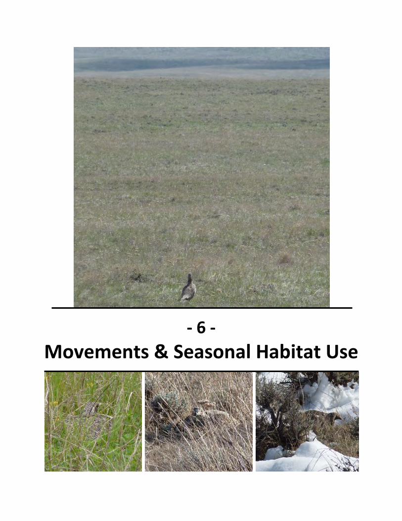
- 6 -

Movements & Seasonal Habitat Use

57

INTRODUCTION

Sage-grouse exhibit a wide range of movement strategies, from using a single home

range year-round to using multiple distinct seasonal ranges (Connelly et al. 2011b, Tack et al.

2011). Movements of up to 100 miles between seasonal ranges have been documented (Smith

2013). Sage-grouse seasonal movements may be driven by necessity (e.g. to access winter

range in a fragmented landscape), but even within large expanses of prime habitat, sage-grouse

may bypass suitable habitat to return to traditional ranges learned during their first year of life

(Berry and Eng 1985, Connelly et al. 1988, Schroeder and Robb 2003).

Sage-grouse core areas in Montana were delineated based solely on lek locations and

associated male counts (Chapter 1). Little was known about habitat use and movements of

sage-grouse during the rest of their annual cycle. It was unknown if the Core Area (Fig. 1.2), as

delineated, was adequate to meet the year-round needs of sage-grouse. Are sage-grouse

observed on leks in the Core Area moving outside the boundaries of the Core Area to meet

their seasonal needs? Should the boundary of the Core Area be adjusted to accommodate

seasonal movements? Because important areas for sage-grouse are a function of both habitat

and tradition (i.e., learned areas), tracking collared sage-grouse was necessary to understand

sage-grouse use of the landscape.

Our objective was to quantify seasonal movements, site fidelity, and habitat use of sage-

grouse within the Core Area to better understand how resident grouse use the landscape year-

round and assess the adequacy of the Core Area, as delineated, to accommodate the life history

needs of denizen grouse. The resulting information will help managers prioritize sage-grouse

conservation efforts at a landscape level and compose sound recommendations to minimize

the impacts of development and associated disturbance on resident sage-grouse.

METHODS

Our goal was to monitor radio-collared hens at least once per week from April–

September and twice per month from October–March. Occasionally, hens were monitored less

frequently due to severe weather events or logistical constraints. We used telemetry

58

techniques (Samuel and Fuller 1996) to locate hens on the ground from April–September. We

conducted telemetry flights when hens could not be located on the ground and to locate all

hens from October–March. At each location, we recorded status (e.g., live, nesting, brood-

rearing), GPS location, habitat information, and other pertinent notes.

We recorded >2,800 unique locations for 94 radio-collared hens, thus it was not

logistically feasible to exhaustively measure vegetation at each location. Therefore, we

recorded basic habitat information to quantify seasonal habitat use. For ground and aerial

locations, we classified habitat into 4 categories: sagebrush-steppe (≥1% shrub canopy cover),

grassland (<1% shrub cover), alfalfa (including mixed grass/alfalfa hay fields), and wetland. For

ground locations in sagebrush-steppe we visually estimated shrub canopy cover as 1–10%, 11–

25%, or >25%, and estimated the average height of mature shrubs by taking a single height

measurement of an average shrub. We also recorded whether a hen was located within 100

yards of a water source (e.g., pond, reservoir, creek or wetland) at all ground locations.

Analyses

We calculated the mean lek-to-nest distance and the percentage of hens that nested

within 1, 2, 3, 4, and >4 mi from known leks in the Core Area. We selected these distances

because other research has suggested sage-grouse tend to nest near leks (e.g., Braun et al.

1977) and the BLM commonly restricts activity within these distances to protect nesting grouse

from various levels of disturbance. Female sage-grouse tend to make inter-lek movements

during the breeding season (Dunn and Braun 1985), so we did not restrict analyses to the lek

nearest a hen’s capture location. However, this method may underestimate lek-to-nest

distances because we did not confirm that hens visited the lek nearest to their nest location,

nor was every lek surveyed every year to confirm activity. To better understand this bias, we

calculated the distances between nests and leks known to be active during the study for a

portion of the Core Area (the Draft Carter County Master Lease Plan [MLP] area; BLM 2013)

that was exhaustively surveyed for leks each year. The MLP area comprises 29% of the Core

Area.

59

To examine nesting-area fidelity, we calculated the median and range of distances

between nests within a nesting season and among years for individual hens that nested more

than once during the study. For brood hens, we calculated the mean and range of distances

from nest locations to brood-rearing locations at 14 and 30 days post-hatch. Distances were

calculated using Hawth’s Tools (Beyer 2004) in ArcGIS 9.3 (Environmental Systems Research

Institute, Redlands, CA).

We examined movements for each hen to determine if distinct seasonal ranges were

used. We excluded data from hens that died before seasonal ranges could be established. An

area was considered a distinct seasonal range if the hen was located in an area for several

weeks with no overlapping locations during other seasons. We provide summaries of hen

annual and seasonal movements, including number of seasonal ranges utilized, maximum

length of seasonal ranges, distances moved between seasonal ranges, and the median date of

movements between ranges. Distances (center to center) were calculated using the measure

tool in ArcGIS 9.3 (Environmental Systems Research Institute, Redlands, CA).

We calculated minimum convex polygons (MCP) for hens that were tracked >1 year

using Hawth’s Tools. One hen that was tracked >1 year was excluded from MCP analysis

because a malfunctioning radio collar resulted in large data gaps and a MCP that was biased

small. Although MCPs are not accurate home-range size estimates (i.e. not all areas within an

MCP are used by a hen), they provide a measure of how large of an area hens are using on the

landscape. We include figures showing example movement patterns and MCPs. To assess the

adequacy of the size of the Core Area to accommodate the life history needs of resident grouse,

we present figures showing the overall dispersion of study hens during spring–fall (March 1–

October 28) and winter (November 1–February 28) overlaid with core and connectivity area

delineations from South Dakota (South Dakota Game, Fish, and Parks unpublished draft sage-

grouse core area delineations obtained December 2013) and Wyoming (Wyoming Game and

Fish Department 2010).

To better understand the influence of winter severity on sage-grouse movements, we

calculated the average distance moved between each within-winter telemetry survey and total

point-to-point distances moved by year using hens as sampling units. It was necessary to

60

calculate both of these metrics because the number of winter telemetry flights varied among

years, which confounds comparison of movements among winters. Higher survey frequency

would be expected to increase total distance moved but decrease the average distance moved

between consecutive within-winter telemetry surveys. For 30 hens that were tracked >1

winter, we examined fidelity to winter range and calculated the average distance between

winter ranges when different wintering areas were used.

To examine seasonal habitat use, we compiled data on habitat variables for each hen for

4 seasons: breeding (March 1–April 15), nesting/brood-rearing (April 16–July 15), late

summer/fall (July 16–October 31), and winter (November 1–February 28). We further divided

the nesting/brood-rearing season based on a hen’s status into prenesting, nesting, early brood-

rearing (hatch–30 days post-hatch), late brood-rearing (>30 days post-hatch), and broodless

hens (for hens who did not initiate nests or following nest or brood failure). We treated hens as

sampling units and calculated averages for each habitat variable for each season/status.

RESULTS

Movements

The average distance between sage-grouse nests and known leks was 1.15 miles (SE =

0.13 miles). Fifty-nine percent (90/152) of nests were within one mile of a lek, 84% (127/152)

within 2 miles, 93% (142/152) within 3 miles, and 97% (147/152) within 4 miles. All nests were

within 5.0 miles of a lek. When analyses were restricted to known-active leks in the MLP area,

47% (25/53) of nests were within one mile of a known active lek, 68% (36/53) were within 2

miles, 88% (46/53) were within 3 miles, and 92% (49/53) were within 4 miles. All nests were

within 4.6 miles of an active lek in the MLP. Hens generally exhibited nesting area fidelity; the

overall median distance between nests was 0.28 mi (Table 6.1). The overall range of between-

year nest distances was much larger for yearlings than adults (Table 6.1). Hens moved an

average of 0.53 mile from nests in the first 14 days post-hatch, and 0.68 mile 30 days post-

hatch. The maximum distance traveled from the nest by a brooding hen in the first 30 days was

3.17 miles (Table 6.2).

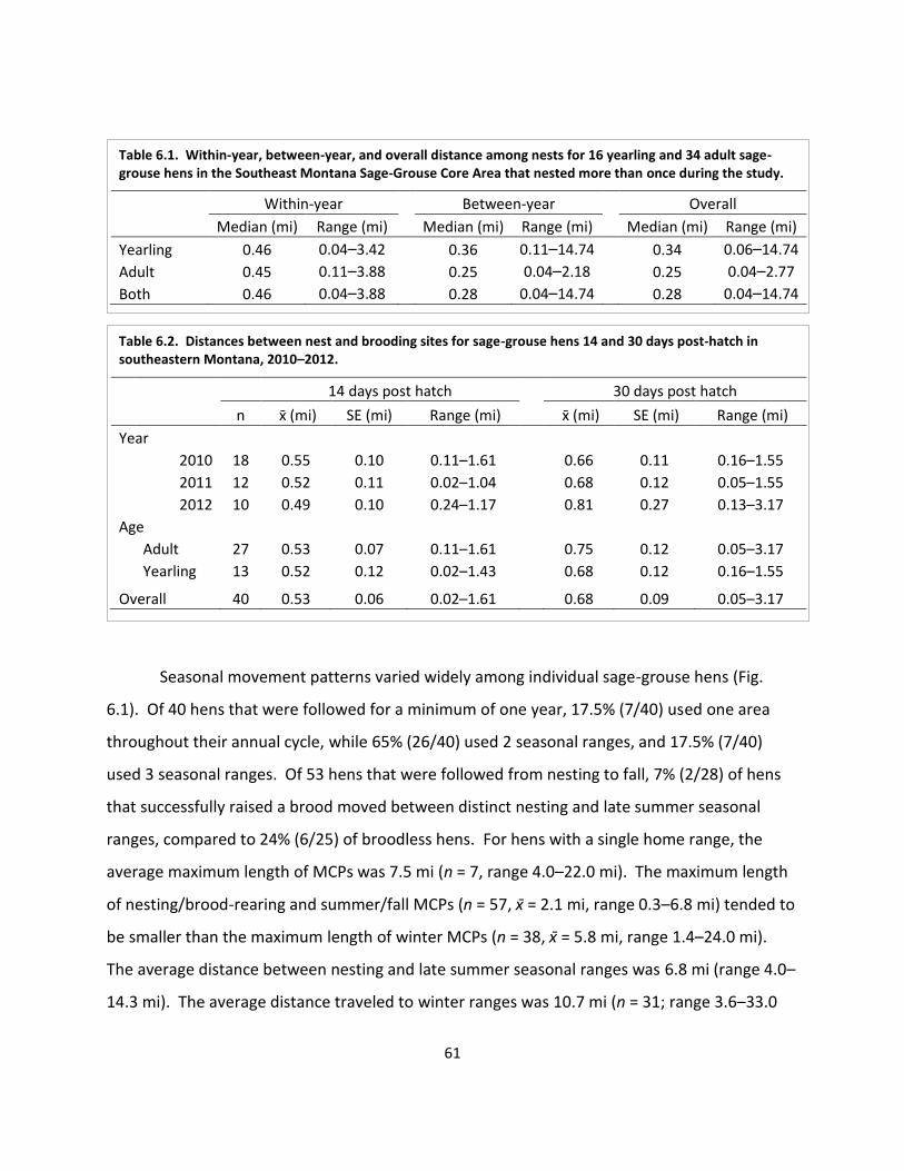
61

Seasonal movement patterns varied widely among individual sage-grouse hens (Fig.

6.1). Of 40 hens that were followed for a minimum of one year, 17.5% (7/40) used one area

throughout their annual cycle, while 65% (26/40) used 2 seasonal ranges, and 17.5% (7/40)

used 3 seasonal ranges. Of 53 hens that were followed from nesting to fall, 7% (2/28) of hens

that successfully raised a brood moved between distinct nesting and late summer seasonal

ranges, compared to 24% (6/25) of broodless hens. For hens with a single home range, the

average maximum length of MCPs was 7.5 mi (n = 7, range 4.0–22.0 mi). The maximum length

of nesting/brood-rearing and summer/fall MCPs (n = 57, = 2.1 mi, range 0.3–6.8 mi) tended to

be smaller than the maximum length of winter MCPs (n = 38, = 5.8 mi, range 1.4–24.0 mi).

The average distance between nesting and late summer seasonal ranges was 6.8 mi (range 4.0–

14.3 mi). The average distance traveled to winter ranges was 10.7 mi (n = 31; range 3.6–33.0

Table 6.2. Distances between nest and brooding sites for sage-grouse hens 14 and 30 days post-hatch in southeastern Montana, 2010–2012.

14 days post hatch

30 days post hatch

n x (mi) SE (mi) Range (mi)

x (mi) SE (mi) Range (mi)

Year

2010 18 0.55 0.10 0.11–1.61

0.66 0.11 0.16–1.55

2011 12 0.52 0.11 0.02–1.04

0.68 0.12 0.05–1.55

2012 10 0.49 0.10 0.24–1.17

0.81 0.27 0.13–3.17

Age

Adult 27 0.53 0.07 0.11–1.61

0.75 0.12 0.05–3.17

Yearling 13 0.52 0.12 0.02–1.43

0.68 0.12 0.16–1.55

Overall 40 0.53 0.06 0.02–1.61 0.68 0.09 0.05–3.17

Table 6.1. Within-year, between-year, and overall distance among nests for 16 yearling and 34 adult sage-grouse hens in the Southeast Montana Sage-Grouse Core Area that nested more than once during the study.

Within-year

Between-year

Overall

Median (mi) Range (mi)

Median (mi) Range (mi)

Median (mi) Range (mi)

Yearling 0.46 0.04–3.42

0.36 0.11–14.74

0.34 0.06–14.74

Adult 0.45 0.11–3.88

0.25 0.04–2.18

0.25 0.04–2.77

Both 0.46 0.04–3.88

0.28 0.04–14.74

0.28 0.04–14.74

62

mi). The median date of movements from either a summer or fall range to a winter range was

October 15 (range September 10–November 15), and the median date of movements from

winter ranges to nesting/summer ranges was March 20 (range March 12–June 3). The average

minimum convex polygon size for hens that were tracked ≥1 year was 71.2 mi2 (SE = 8.8 mi2,

range 7.9–238.1 mi2; see Fig. 6.2 for examples). The overall dispersion of radio-collared hens

during the breeding through fall seasons (March 1 to October 31) and winter (November 1–

February 28) are pictured in Figures 6.3 and 6.4.

The average distance moved between telemetry surveys and total distance moved over

winter were greater during winters 2009–10 and 2010–11 than milder 2011–12 or 2012–13

winters (Table 6.3). Fifty-four percent (12/22) of hens used a different winter range during the

extreme 2010–11 winter than either the previous or following winters (Table 6.4). Four of

these hens used a single home range year-round except during the severe winter. In

comparison, only 18% (3/17) of hens used a different winter range during the mild 2011–12

winter compared with the average 2012–13 winter. The average distance between winter

range for 15 hens that used different areas between years was 8.6 miles (SE = 1.1 mi, range =

3.6–17.5 mi). Many of the hens that used a different range during the severe winter moved

there after beginning winter from the same winter range used during milder winters.

Seasonal Habitat Use

Seasonal habitat use is summarized in Table 6.5. More than 98% of sage-grouse

locations during breeding, prenesting, nesting, and winter were in sagebrush-steppe habitat,

compared to 79–83% of locations during brood-rearing. Sage-grouse tended to use dense

stands of sagebrush (>25% canopy cover) in the greatest proportion during prenesting and

nesting, and moderate density sagebrush (11–25% canopy cover) in the greatest proportion

during winter and breeding. Sage-grouse tended to be located adjacent to water sources or

wetlands most often during the late brood-rearing period.

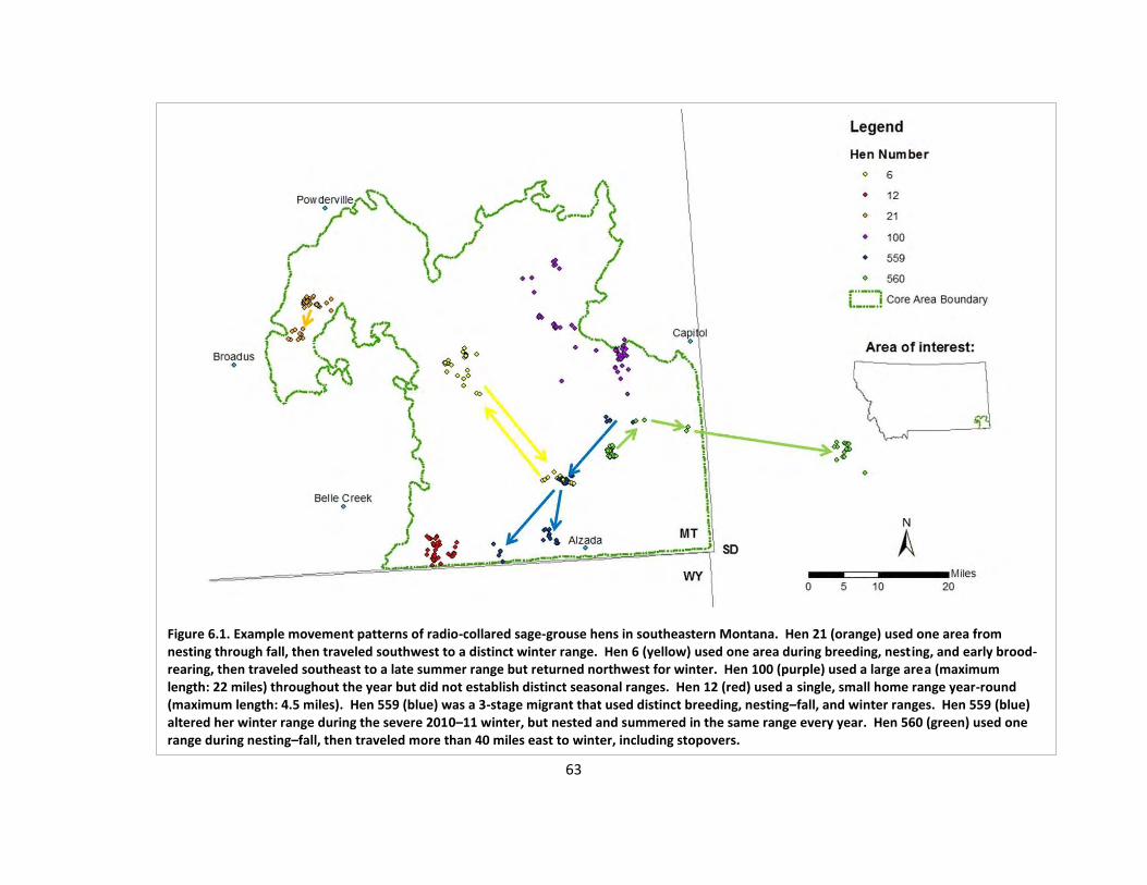
63

Figure 6.1. Example movement patterns of radio-collared sage-grouse hens in southeastern Montana. Hen 21 (orange) used one area from nesting through fall, then traveled southwest to a distinct winter range. Hen 6 (yellow) used one area during breeding, nesting, and early brood-rearing, then traveled southeast to a late summer range but returned northwest for winter. Hen 100 (purple) used a large area (maximum length: 22 miles) throughout the year but did not establish distinct seasonal ranges. Hen 12 (red) used a single, small home range year-round (maximum length: 4.5 miles). Hen 559 (blue) was a 3-stage migrant that used distinct breeding, nesting–fall, and winter ranges. Hen 559 (blue) altered her winter range during the severe 2010–11 winter, but nested and summered in the same range every year. Hen 560 (green) used one range during nesting–fall, then traveled more than 40 miles east to winter, including stopovers.

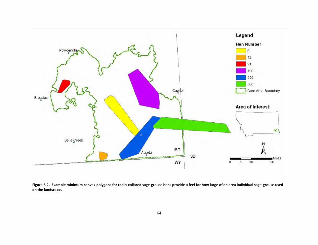
64

Figure 6.2. Example minimum convex polygons for radio-collared sage-grouse hens provide a feel for how large of an area individual sage-grouse used on the landscape.

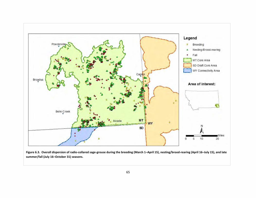
65

Figure 6.3. Overall dispersion of radio-collared sage-grouse during the breeding (March 1–April 15), nesting/brood-rearing (April 16–July 15), and late

summer/fall (July 16–October 31) seasons.

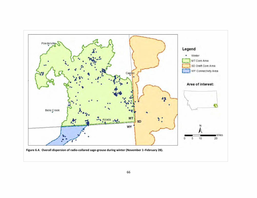
66

Figure 6.4. Overall dispersion of radio-collared sage-grouse during winter (November 1–February 28).

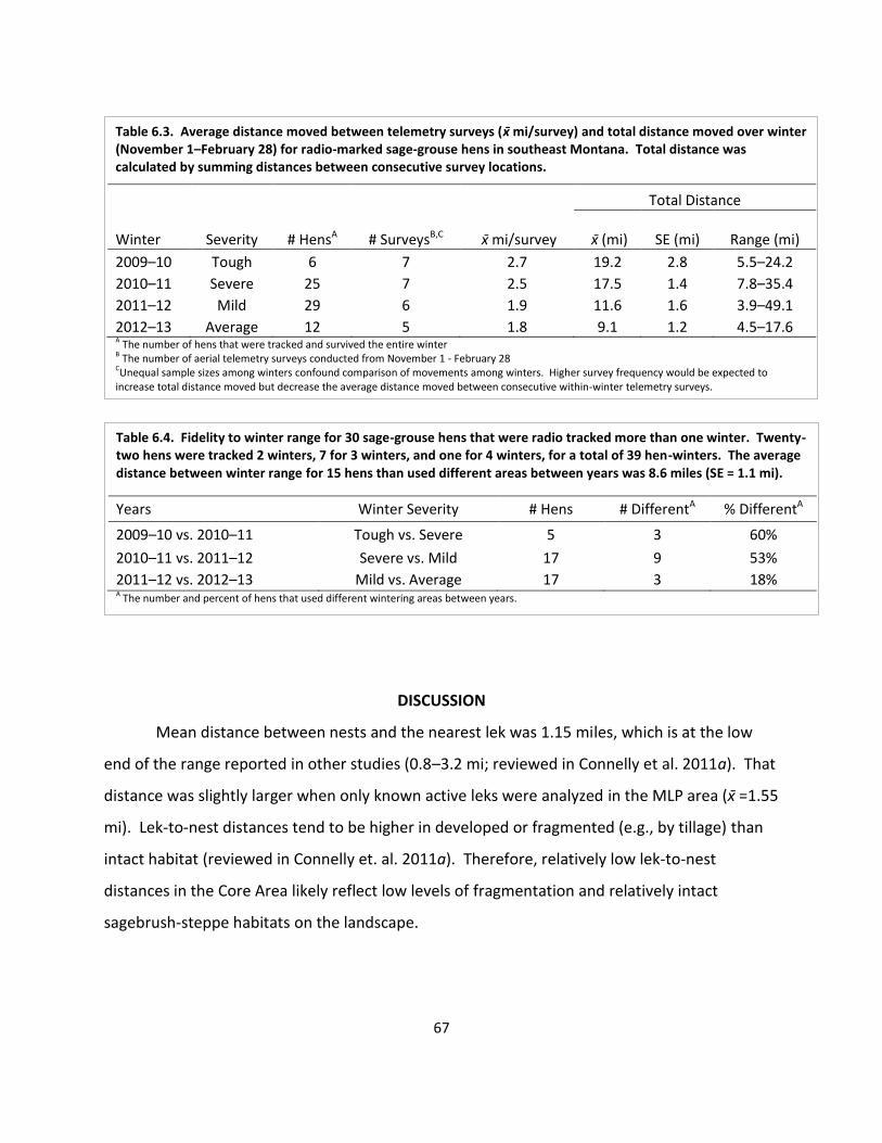
67

DISCUSSION

Mean distance between nests and the nearest lek was 1.15 miles, which is at the low

end of the range reported in other studies (0.8–3.2 mi; reviewed in Connelly et al. 2011a). That

distance was slightly larger when only known active leks were analyzed in the MLP area ( =1.55

mi). Lek-to-nest distances tend to be higher in developed or fragmented (e.g., by tillage) than

intact habitat (reviewed in Connelly et. al. 2011a). Therefore, relatively low lek-to-nest

distances in the Core Area likely reflect low levels of fragmentation and relatively intact

sagebrush-steppe habitats on the landscape.

Table 6.4. Fidelity to winter range for 30 sage-grouse hens that were radio tracked more than one winter. Twenty-two hens were tracked 2 winters, 7 for 3 winters, and one for 4 winters, for a total of 39 hen-winters. The average distance between winter range for 15 hens than used different areas between years was 8.6 miles (SE = 1.1 mi).

Years Winter Severity # Hens # DifferentA % DifferentA

2009–10 vs. 2010–11 Tough vs. Severe 5 3 60%

2010–11 vs. 2011–12 Severe vs. Mild 17 9 53%

2011–12 vs. 2012–13 Mild vs. Average 17 3 18% A The number and percent of hens that used different wintering areas between years.

Table 6.3. Average distance moved between telemetry surveys ( mi/survey) and total distance moved over winter (November 1–February 28) for radio-marked sage-grouse hens in southeast Montana. Total distance was calculated by summing distances between consecutive survey locations.

Total Distance

Winter

Severity # HensA # SurveysB,C mi/survey (mi) SE (mi) Range (mi)

2009–10 Tough 6 7 2.7 19.2 2.8 5.5–24.2

2010–11 Severe 25 7 2.5 17.5 1.4 7.8–35.4

2011–12 Mild 29 6 1.9 11.6 1.6 3.9–49.1

2012–13 Average 12 5 1.8 9.1 1.2 4.5–17.6 A The number of hens that were tracked and survived the entire winter B The number of aerial telemetry surveys conducted from November 1 - February 28 CUnequal sample sizes among winters confound comparison of movements among winters. Higher survey frequency would be expected to increase total distance moved but decrease the average distance moved between consecutive within-winter telemetry surveys.

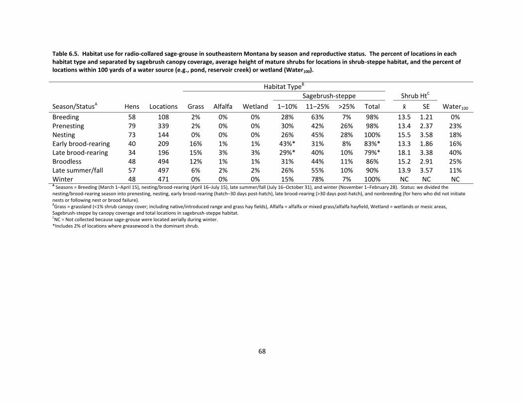
68

Table 6.5. Habitat use for radio-collared sage-grouse in southeastern Montana by season and reproductive status. The percent of locations in each habitat type and separated by sagebrush canopy coverage, average height of mature shrubs for locations in shrub-steppe habitat, and the percent of locations within 100 yards of a water source (e.g., pond, reservoir creek) or wetland (Water100).

Habitat TypeB

Sagebrush-steppe Shrub HtC

Season/StatusA Hens Locations Grass Alfalfa Wetland 1–10% 11–25% >25% Total x SE Water100

Breeding 58 108 2% 0% 0% 28% 63% 7% 98% 13.5 1.21 0% Prenesting 79 339 2% 0% 0% 30% 42% 26% 98% 13.4 2.37 23% Nesting 73 144 0% 0% 0% 26% 45% 28% 100% 15.5 3.58 18% Early brood-rearing 40 209 16% 1% 1% 43%* 31% 8% 83%* 13.3 1.86 16% Late brood-rearing 34 196 15% 3% 3% 29%* 40% 10% 79%* 18.1 3.38 40% Broodless 48 494 12% 1% 1% 31% 44% 11% 86% 15.2 2.91 25% Late summer/fall 57 497 6% 2% 2% 26% 55% 10% 90% 13.9 3.57 11% Winter 48 471 0% 0% 0% 15% 78% 7% 100% NC NC NC A Seasons = Breeding (March 1–April 15), nesting/brood-rearing (April 16–July 15), late summer/fall (July 16–October 31), and winter (November 1–February 28). Status: we divided the nesting/brood-rearing season into prenesting, nesting, early brood-rearing (hatch–30 days post-hatch), late brood-rearing (>30 days post-hatch), and nonbreeding (for hens who did not initiate nests or following nest or brood failure). BGrass = grassland (<1% shrub canopy cover; including native/introduced range and grass hay fields), Alfalfa = alfalfa or mixed grass/alfalfa hayfield, Wetland = wetlands or mesic areas, Sagebrush-steppe by canopy coverage and total locations in sagebrush-steppe habitat. CNC = Not collected because sage-grouse were located aerially during winter. *Includes 2% of locations where greasewood is the dominant shrub.

69

Restriction radii surrounding leks for surface disturbing activities typically range from

1.0–4.0 mi, and 59% of nests were within one mile of a known lek location, 84% within 2 miles,

93% within 3 miles, and 97% within 4 miles. These percentages were lower when only known

active leks were considered: only 47% of nests were found within one mile of a lek, but the

majority (92%) of nests were still found within 4 miles of an active lek. Nest success exerts

great influence on population growth rates for sage-grouse. Therefore, a one-mile buffer is

inadequate to avoid significant population impacts associated with development activities. We

recommend a minimum 4 mile buffer for highly-intrusive practices within suitable sagebrush

habitat. Brood hens tended to stay close to nest sites for the first 30 days following hatch ( =

0.68 mi), and thus restrictive radii placed around leks to protect nesting habitat may also

benefit young broods.

Sage-grouse exhibited strong nest site fidelity. The median distance between nests and

renests (0.46 mi) and the median distance between consecutive-year nests (0.28 mi) were

lower than reported in other studies (1.2–1.6 mi between nests and renests, 0.4–1.9 mi

between consecutive-year nests; reviewed in Connelly et al. 2011a). Median distances

between nests were only slightly larger for yearlings (0.34 mi) than adults (0.25 mi), which

indicates that nesting sage-grouse often exhibit fidelity to their first nesting location. However,

the maximum distance between nests was much larger for yearlings (14.74 mi) than adults

(3.88 mi), which indicates that young hens may, in some cases, exhibit considerable plasticity

with regard to nesting locations.

Brood hens moved an average 0.68 mile during the first 30 days post hatch, which is

similar to movements reported in other studies ( = 0.49–0.93 mi; reviewed in Connelly et al.

2011a). Movements during the first 14 days post-hatch were similar among years ( = 0.53 mi,

maximum = 1.61 mi), but the average and maximum distance moved by 30 days post-hatch was

greater in drought year 2012 ( = 0.81, max = 3.2 mi) than other years ( < 0.68 mi, max = 1.6

mi). This suggests that brood movements are limited by chick motility during the first 14 days

post-hatch (Schroeder et al. 1999), but that by 30 days post-hatch hens may move broods

longer distances to find higher quality foraging habitat during dry years.

70

As summer progressed and vegetation in uplands desiccated, both brood and broodless

hens tended to move to more mesic areas, and used non-sagebrush habitats (e.g., grasslands,

wetlands, alfalfa fields) in greater proportion, which has been well-documented in sage-grouse

(Klebenow 1969, Martin 1970, Peterson 1970, Wallestad 1971). Interestingly, brood hens were

less likely to move to distinct late summer ranges (7%; 2/28) than broodless hens (6/25; 24%),

which would suggest that chicks may continue to have limited motility during late summer.

However, late brooding hens were found more often in non-sagebrush mesic habitats than

broodless hens, which suggests that high-quality brood-rearing habitat was available for brood

hens in close proximity to nesting/early brood-rearing locations. We suspect that late summer

movements by broodless hens may be driven by other factors (e.g., that hens may be searching

for other broodless hens to flock with), or that the trend for broodless hens to be more likely to

use distinct late summer ranges may be an artifact of small sample size.

Sage-grouse are sagebrush obligates that depend on sagebrush for food and cover

throughout their annual cycle (Patterson 1952, Dalke et al. 1963). More than 79% of locations

in any season, and >98% of locations during breeding, prenesting, nesting, and winter were in

sagebrush-steppe habitat, similar to sage-grouse elsewhere (Connelly et al. 2011c). Sage-

grouse tended to use dense stands sagebrush (>25% canopy cover) in the greatest proportion

during prenesting and nesting, and moderate density sagebrush (11–25% canopy cover) in the

greatest proportion during winter and breeding. This moderate to dense sagebrush is

oftentimes what people think of when they visualize sage-grouse habitat, yet sage-grouse

frequently (>25% of locations) used areas with sparse (1–10% canopy cover) sagebrush during

spring through fall. Even during winter, 15% of locations were sagebrush with <10% canopy

cover. Observed patterns of habitat use in the Core Area likely reflect habitat availability for a

population on the eastern edge of the range, but nevertheless highlight the importance of

heterogeneous (including areas with dense, moderate, and sparse canopy cover) sagebrush

habitat to resident sage-grouse.

Movement patterns for individual sage-grouse hens varied greatly in the Core Area. A

majority (60%) of hens tracked >1 year made movements >6.2 miles, often used as the

definition of a migratory population (Connelly et al. 2000b). Yet, roughly 18% made no

71

movements at all between seasonal ranges, and many traveled <6.2 miles between ranges.

Fifty-four percent of hens utilized different winter ranges and movement patterns during the

severe 2010–11 winter compared with previous or subsequent winters, and 4 hens were non-

migratory except during the severe winter. Variation in migratory strategies within populations

has been documented for sage-grouse (e.g., Swanson 2009, Fedy et al. 2012), as has plasticity

related to severe winter events (Smith 2013).

The majority of locations of collared sage-grouse fell within the boundary of the Core

Area in Montana, but many hens made movements into areas of South Dakota and Wyoming

adjacent to the Core Area. Similarly, Swanson (2009) documented movements of radio-collared

sage-grouse between South Dakota and the Core Area. Cooperation among states will be

necessary to maintain sagebrush habitat on the landscape and manage this sage-grouse

population across state borders. Sage-grouse core/connectivity areas provide excellent

framework to cooperatively manage sage-grouse populations across administrative boundaries.

South Dakota draft core areas encompassed nearly all locations from radio-collared sage-

grouse hens. However, core area boundaries for Montana and South Dakota do not match up

near the historic town of Capitol, Montana. Locations of collared sage-grouse in the area,

including a handful of locations between the 2 core areas, suggest the area is important from a

connectivity standpoint. Therefore, we recommend that the Montana Core Area be expanded

to include suitable sagebrush habitat south of the Little Missouri River and Hackberry Creek.

For hens that moved into adjacent areas of Wyoming, the majority of locations were within a

connectivity area, but many locations were outside of the connectivity area to the east,

including important and critical winter range (Fig. 7.1). We recommend the Wyoming

connectivity area be expanded to incorporate sage-grouse winter range delineated in Figure

7.1. Similarly, 3 winter range polygons (Fig. 7.1) extended <1.75 miles outside of the Core Area

in Montana and should be included in the Core Area delineation.

- 7 -

Winter Use & Vegetation

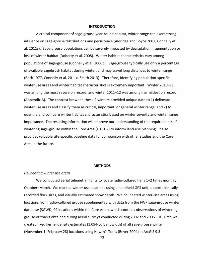
73

INTRODUCTION

A critical component of sage-grouse year-round habitat, winter range can exert strong

influence on sage-grouse distributions and persistence (Aldridge and Boyce 2007, Connelly et

al. 2011c). Sage-grouse populations can be severely impacted by degradation, fragmentation or

loss of winter habitat (Doherty et al. 2008). Winter habitat characteristics vary among

populations of sage-grouse (Connelly et al. 2000b). Sage-grouse typically use only a percentage

of available sagebrush habitat during winter, and may travel long distances to winter range

(Beck 1977, Connelly et al. 2011c, Smith 2013). Therefore, identifying population-specific

winter use areas and winter habitat characteristics is extremely important. Winter 2010–11

was among the most severe on record, and winter 2011–12 was among the mildest on record

(Appendix A). The contrast between these 2 winters provided unique data to 1) delineate

winter use areas and classify them as critical, important, or general winter range, and 2) to

quantify and compare winter habitat characteristics based on winter severity and winter range

importance. The resulting information will improve our understanding of the requirements of

wintering sage-grouse within the Core Area (Fig. 1.2) to inform land-use planning. It also

provides valuable site-specific baseline data for comparison with other studies and the Core

Area in the future.

METHODS

Delineating winter use areas

We conducted aerial telemetry flights to locate radio-collared hens 1–2 times monthly

October–March. We marked winter use locations using a handheld GPS unit, opportunistically

recorded flock sizes, and visually estimated snow depth. We delineated winter-use areas using

locations from radio-collared grouse supplemented with data from the FWP sage-grouse winter

database (SGWD; 99 locations within the Core Area), which contains observations of wintering

grouse or tracks obtained during aerial surveys conducted during 2002 and 2006–10. First, we

created fixed kernel density estimates (1,094-yd bandwidth) of all sage-grouse winter

(November 1–February 28) locations using Hawth’s Tools (Beyer 2004) in ArcGIS 9.3

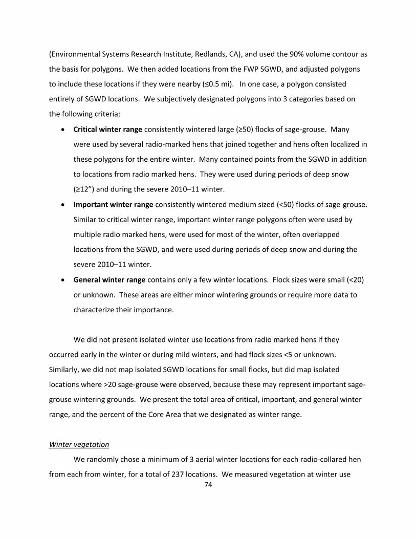
74

(Environmental Systems Research Institute, Redlands, CA), and used the 90% volume contour as

the basis for polygons. We then added locations from the FWP SGWD, and adjusted polygons

to include these locations if they were nearby (≤0.5 mi). In one case, a polygon consisted

entirely of SGWD locations. We subjectively designated polygons into 3 categories based on

the following criteria:

Critical winter range consistently wintered large (≥50) flocks of sage-grouse. Many

were used by several radio-marked hens that joined together and hens often localized in

these polygons for the entire winter. Many contained points from the SGWD in addition

to locations from radio marked hens. They were used during periods of deep snow

(≥12”) and during the severe 2010–11 winter.

Important winter range consistently wintered medium sized (<50) flocks of sage-grouse.

Similar to critical winter range, important winter range polygons often were used by

multiple radio marked hens, were used for most of the winter, often overlapped

locations from the SGWD, and were used during periods of deep snow and during the

severe 2010–11 winter.

General winter range contains only a few winter locations. Flock sizes were small (<20)

or unknown. These areas are either minor wintering grounds or require more data to

characterize their importance.

We did not present isolated winter use locations from radio marked hens if they

occurred early in the winter or during mild winters, and had flock sizes <5 or unknown.

Similarly, we did not map isolated SGWD locations for small flocks, but did map isolated

locations where >20 sage-grouse were observed, because these may represent important sage-

grouse wintering grounds. We present the total area of critical, important, and general winter

range, and the percent of the Core Area that we designated as winter range.

Winter vegetation

We randomly chose a minimum of 3 aerial winter locations for each radio-collared hen

from each from winter, for a total of 237 locations. We measured vegetation at winter use

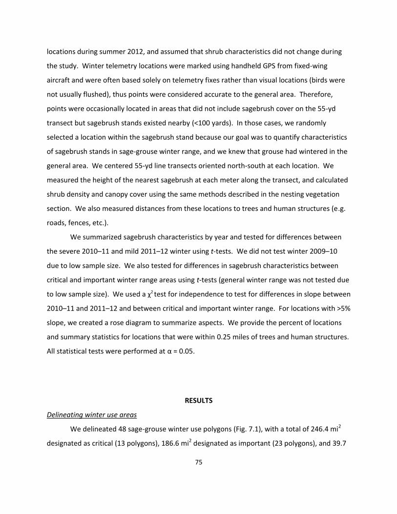
75

locations during summer 2012, and assumed that shrub characteristics did not change during

the study. Winter telemetry locations were marked using handheld GPS from fixed-wing

aircraft and were often based solely on telemetry fixes rather than visual locations (birds were

not usually flushed), thus points were considered accurate to the general area. Therefore,

points were occasionally located in areas that did not include sagebrush cover on the 55-yd

transect but sagebrush stands existed nearby (<100 yards). In those cases, we randomly

selected a location within the sagebrush stand because our goal was to quantify characteristics

of sagebrush stands in sage-grouse winter range, and we knew that grouse had wintered in the

general area. We centered 55-yd line transects oriented north-south at each location. We

measured the height of the nearest sagebrush at each meter along the transect, and calculated

shrub density and canopy cover using the same methods described in the nesting vegetation

section. We also measured distances from these locations to trees and human structures (e.g.

roads, fences, etc.).

We summarized sagebrush characteristics by year and tested for differences between

the severe 2010–11 and mild 2011–12 winter using t-tests. We did not test winter 2009–10

due to low sample size. We also tested for differences in sagebrush characteristics between

critical and important winter range areas using t-tests (general winter range was not tested due

to low sample size). We used a χ2 test for independence to test for differences in slope between

2010–11 and 2011–12 and between critical and important winter range. For locations with >5%

slope, we created a rose diagram to summarize aspects. We provide the percent of locations

and summary statistics for locations that were within 0.25 miles of trees and human structures.

All statistical tests were performed at α = 0.05.

RESULTS

Delineating winter use areas

We delineated 48 sage-grouse winter use polygons (Fig. 7.1), with a total of 246.4 mi2

designated as critical (13 polygons), 186.6 mi2 designated as important (23 polygons), and 39.7

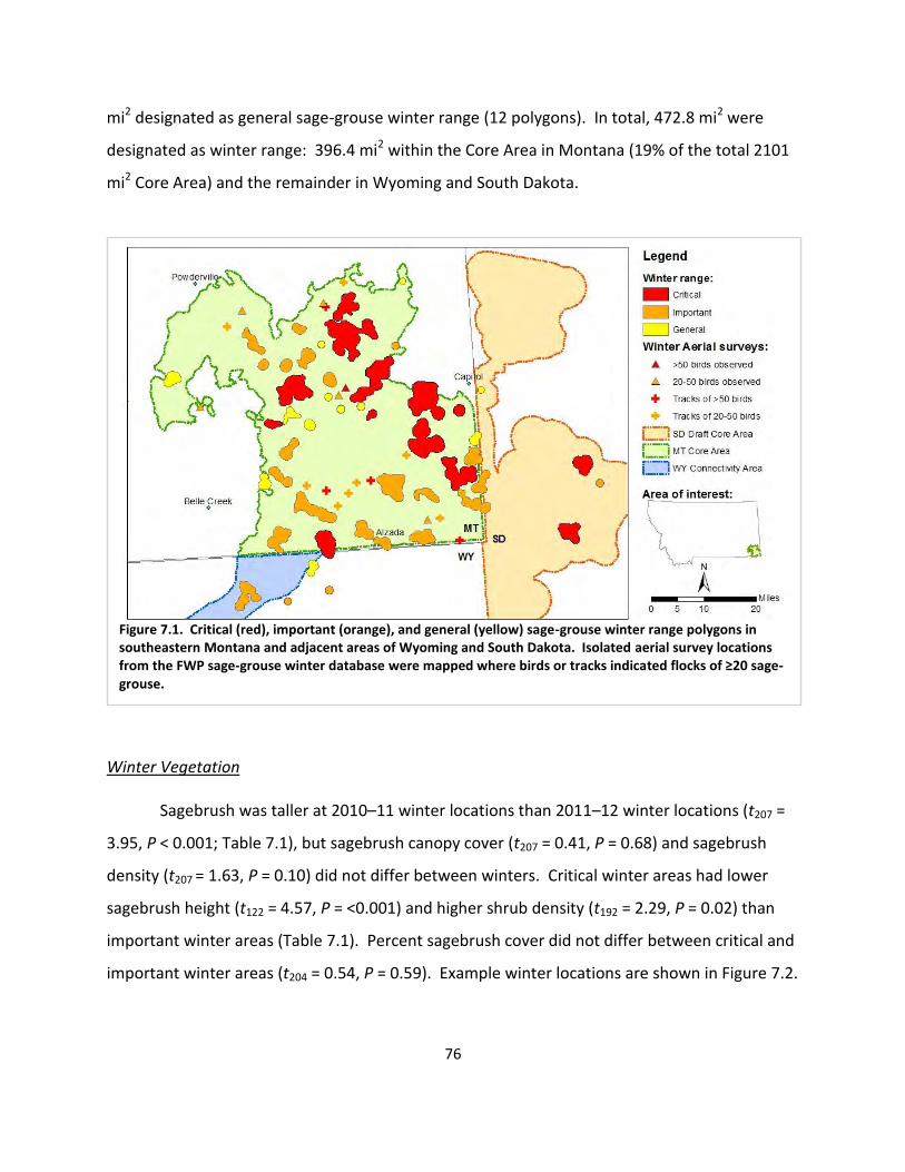
76

mi2 designated as general sage-grouse winter range (12 polygons). In total, 472.8 mi2 were

designated as winter range: 396.4 mi2 within the Core Area in Montana (19% of the total 2101

mi2 Core Area) and the remainder in Wyoming and South Dakota.

Winter Vegetation

Sagebrush was taller at 2010–11 winter locations than 2011–12 winter locations (t207 =

3.95, P < 0.001; Table 7.1), but sagebrush canopy cover (t207 = 0.41, P = 0.68) and sagebrush

density (t207 = 1.63, P = 0.10) did not differ between winters. Critical winter areas had lower

sagebrush height (t122 = 4.57, P = <0.001) and higher shrub density (t192 = 2.29, P = 0.02) than

important winter areas (Table 7.1). Percent sagebrush cover did not differ between critical and

important winter areas (t204 = 0.54, P = 0.59). Example winter locations are shown in Figure 7.2.

Figure 7.1. Critical (red), important (orange), and general (yellow) sage-grouse winter range polygons in southeastern Montana and adjacent areas of Wyoming and South Dakota. Isolated aerial survey locations from the FWP sage-grouse winter database were mapped where birds or tracks indicated flocks of ≥20 sage-grouse.

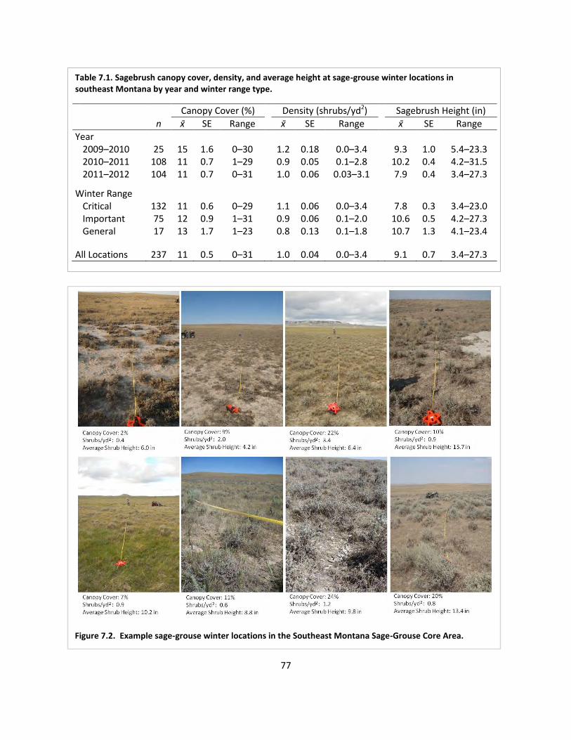
77

Table 7.1. Sagebrush canopy cover, density, and average height at sage-grouse winter locations in southeast Montana by year and winter range type.

Canopy Cover (%) Density (shrubs/yd2) Sagebrush Height (in)

n SE Range SE Range SE Range

Year 2009–2010 25 15 1.6 0–30 1.2 0.18 0.0–3.4 9.3 1.0 5.4–23.3 2010–2011 108 11 0.7 1–29 0.9 0.05 0.1–2.8 10.2 0.4 4.2–31.5 2011–2012 104 11 0.7 0–31 1.0 0.06 0.03–3.1 7.9 0.4 3.4–27.3

Winter Range

Critical 132 11 0.6 0–29 1.1 0.06 0.0–3.4 7.8 0.3 3.4–23.0 Important 75 12 0.9 1–31 0.9 0.06 0.1–2.0 10.6 0.5 4.2–27.3 General 17 13 1.7 1–23 0.8 0.13 0.1–1.8 10.7 1.3 4.1–23.4

All Locations 237 11 0.5 0–31

1.0 0.04 0.0–3.4

9.1 0.7 3.4–27.3

Figure 7.2. Example sage-grouse winter locations in the Southeast Montana Sage-Grouse Core Area.

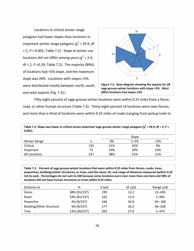
78

Table 7.3. Percent of sage-grouse winter locations that were within 0.25 miles from fences, roads, trees, powerlines, buildings/other structures, or trees, and the mean, SE, and range of distances measured (within 0.25 mi) to each. Percentages do not sum to 100 because some locations were near more than one item and 38% of locations did not have human structures or trees within 0.25 miles.

Distance to % (yd) SE (yd) Range (yd)

Fence 38% (91/237) 199 13.2 21–492

Road 34% (81/237) 163 13.9 1–492

Powerline 4% (9/237) 166 34.8 50– 390

Building/Other Structure 4% (9/237) 177 30.2 66–328

Tree 13% (30/237) 203 27.6 1–470

Locations in critical winter range

polygons had lower slopes than locations in

important winter range polygons (χ2 = 29.9, df

= 2, P < 0.001; Table 7.2). Slope at winter use

locations did not differ among years (χ2 = 2.4,

df = 2, P =0.29; Table 7.2). The majority (89%)

of locations had <5% slope, and the maximum

slope was 20%. Locations with slopes >5%

were distributed mostly between north, south,

and west aspects (Fig. 7.3).

Fifty-eight percent of sage-grouse winter locations were within 0.25 miles from a fence,

road, or other human structure (Table 7.3). Thirty-eight percent of locations were near fences,

and more than a third of locations were within 0.25 miles of roads (ranging from pickup trails to

Table 7.2. Slope was lower in critical versus important sage-grouse winter range polygons (χ2 = 29.9, df = 2, P <

0.001).

Slope

Winter Range n 0% 1–5% >5%

Critical 132 51% 45% 4% Important 75 19% 59% 23% All Locations 237 38% 51% 11%

Figure 7.3. Rose diagram showing the aspects for 28 sage-grouse winter locations with slope >5%. Most (89%) locations had slopes ≤5%

79

highways). Thirteen percent of locations were near trees, typically sparsely-treed creek

bottoms. Few (≤4%) locations were within 0.25 miles from power lines, buildings, or other

human structures.

DISCUSSION

We designated 19% of the Core Area as sage-grouse winter range. We recommend the

Wyoming connectivity area be expanded to incorporate sage-grouse winter range delineated in

Figure 7.1. Similarly, 3 winter range polygons (Fig. 7.1) extended <1.75 miles outside of the

Core Area in Montana and should be included in the Core Area delineation.

The winter use polygons we present provide a strong foundation that land managers

can use to guide management and minimize impacts of development on sage-grouse in the

Core Area. However, the polygons should be viewed as a work-in-progress. As more data

becomes available it may be justified to refine or expand existing polygons, or identify

additional areas as critical or important winter range.

In particular, we were only able to follow one hen from the northeastern portion of the

Core Area. This hen was tracked during mild winters 2011–12 and 2012–13, and remained in

the Core Area throughout winter. Note the single general winter range (yellow) polygon

northeast of Broadus, MT (Fig. 7.4). Based upon sagebrush habitat availability, it is likely that

other sage-grouse winter use areas exist in the Core Area south of Powderville, MT. Several

wintering grounds were identified northwest of Powderville, MT during aerial surveys. We

speculate that sage-grouse from the Core Area might winter in these areas, but more

information is needed. We recommend these wintering areas be given similar protection and

consideration as sage-grouse core areas until more information can be gathered.

Critical sage-grouse winter range was characterized by gentler topography, shorter

shrubs, and greater shrub density than important or general winter range. Similarly, winter use

locations in North and South Dakota were characterized by shorter, denser sagebrush than

random locations (Swanson et al. 2013). These results are contrary to many studies, where

sage-grouse select areas with taller shrubs because sagebrush exposed above snow is necessary

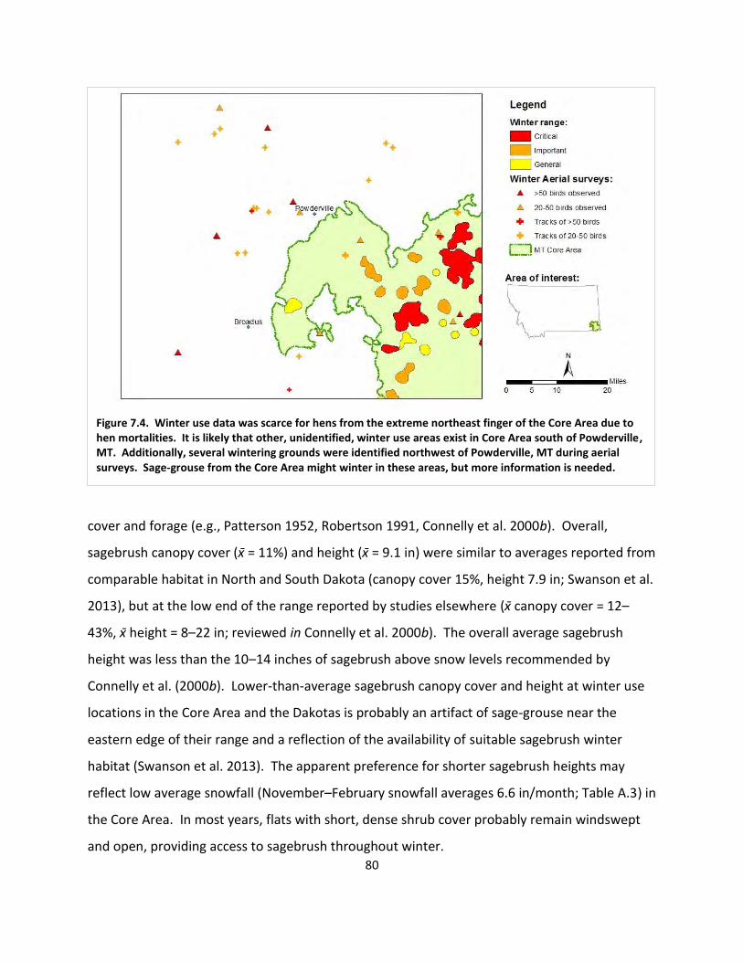
80

cover and forage (e.g., Patterson 1952, Robertson 1991, Connelly et al. 2000b). Overall,

sagebrush canopy cover ( = 11%) and height ( = 9.1 in) were similar to averages reported from

comparable habitat in North and South Dakota (canopy cover 15%, height 7.9 in; Swanson et al.

2013), but at the low end of the range reported by studies elsewhere ( canopy cover = 12–

43%, height = 8–22 in; reviewed in Connelly et al. 2000b). The overall average sagebrush

height was less than the 10–14 inches of sagebrush above snow levels recommended by

Connelly et al. (2000b). Lower-than-average sagebrush canopy cover and height at winter use

locations in the Core Area and the Dakotas is probably an artifact of sage-grouse near the

eastern edge of their range and a reflection of the availability of suitable sagebrush winter

habitat (Swanson et al. 2013). The apparent preference for shorter sagebrush heights may

reflect low average snowfall (November–February snowfall averages 6.6 in/month; Table A.3) in

the Core Area. In most years, flats with short, dense shrub cover probably remain windswept

and open, providing access to sagebrush throughout winter.

Figure 7.4. Winter use data was scarce for hens from the extreme northeast finger of the Core Area due to hen mortalities. It is likely that other, unidentified, winter use areas exist in Core Area south of Powderville, MT. Additionally, several wintering grounds were identified northwest of Powderville, MT during aerial surveys. Sage-grouse from the Core Area might winter in these areas, but more information is needed.

81

Winter 2010–11 was extreme, and snow buried stands of sagebrush throughout much

of the Core Area (Fig. 4.2, Appendix A). As a result, 54% of hens shifted their winter ranges

(Chapter 6). Sagebrush at winter use locations during the severe 2010–11 winter was taller ( =

10.2 in) than during the mild 2011–12 winter ( = 7.9 in). However, we do not suggest that

sagebrush height within winter ranges is a limiting factor for sage-grouse in the Core Area for 3

reasons: 1) Sage-grouse did not necessarily use the tallest or densest sagebrush available.

Even during severe winters, average shrub canopy cover (11%), density (0.9 shrubs/yd2) and

height (10.2 in) were lower than nesting locations which averaged 16% canopy cover, 0.98

shrubs/yd2, and 12.2 in shrub height (Chapter 2). 2) Sagebrush height interacts with

topography to determine sagebrush availability. Taller sagebrush may result in greater snow

drift making food and cover less available to wintering grouse than windswept areas with

shorter sagebrush. 3) Although survival during winter 2010–11 (83%) was lower than other

years (≥95%; Table 4.2), and observations of grouse roosting on a barren snowscape suggested

habitat was limiting during that year (Fig 4.2), a winter that extreme is a rare event (expected

frequency: 1 in 30 years; Appendix A) and has little impact on long-term population growth

rates (Δr = -0.004; Table 5.2).

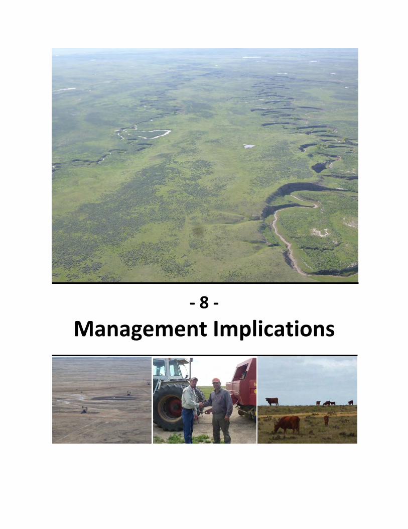
- 8 -

Management Implications

83

Sage-grouse Core Areas comprise <10% of Montana’s land area yet support more than

half of the sage-grouse in the state (NRCS 2010). They are vitally important to the long term

conservation and sustainability of sage-grouse. The Southeastern Montana Sage-grouse Core

Area (Fig. 1.2; hereafter: Core Area) is particularly important because it provides connectivity

with sage-grouse populations in adjacent states and represents a stronghold for sage-grouse

near the eastern edge of their range. Population viability analyses (PVA) suggest that sage-

grouse will continue to persist at sustainable levels in the Core Area unless catastrophic events

(e.g., disease outbreaks) occur and provided the quality and extent of sage-grouse habitat in

the Core Area is maintained or improved (Chapter 5).

Traditional family-owned ranching operations, the predominant local stakeholders in

the Core Area, have historically managed land in a manner that is compatible with sage-grouse

conservation: they have maintained intact sagebrush grasslands. Maintaining this traditional

land use by working with local stakeholders to implement conservation efforts is the most

important management action we can do to ensure the future of sage-grouse in the Core Area.

While ranchers must run profitable operations, they also have a vested interest in the long-

term sustainability of land use practices and are well-poised to collaborate with wildlife and

range professionals to maintain and improve sage-grouse habitat.

To maximize the effectiveness of conservation efforts, stakeholders should consider

organizing planning efforts on a landscape level following the model outlined by Neudecker et

al. (2011) for community-based landscape conservation. This model involves developing

private-public land partnerships that simultaneously benefit local communities, wildlife, and

other natural resources. Under the model, conservation efforts are implemented at the local

scale (e.g., individual ranches), but planning efforts consider the landscape as a whole. We

recommend the following to maintain and enhance sage-grouse habitat in the Core Area:

Maintain Large Expanses of Intact Sagebrush Habitat

Sage-grouse are sagebrush obligates that depend on sagebrush for winter forage (>95%

of winter diet) and year-round cover (Patterson 1952, Dalke et al. 1963, Remington and Braun

1985). Loss, fragmentation and degradation of sagebrush habitat are primary threats to sage-

84

grouse rangewide (USFWS 2010). Future energy development in the Core Area is of concern,

since numerous studies have highlighted the deleterious effects of energy development on

sage-grouse populations (reviewed in Naugle et al. 2011). For example, at well densities >1 well

per square mile, lek losses of 32–77% were documented in Wyoming, which is 2–5 times

greater than losses observed in undeveloped areas (Doherty et al. 2010). The Core Area

currently contains large areas of unfragmented sagebrush-steppe habitat (Montana Sage

Grouse Work Group 2005, Taylor et al. 2010). Therefore, management within the Core Area

should, first and foremost, prioritize maintaining existing sagebrush-steppe habitat by

minimizing habitat loss, fragmentation, and degradation due to factors such as tillage, industrial

development, fire, and herbicide.

Management of sagebrush habitat

When people visualize sage-grouse habitat, they typically think of vast landscapes filled

with tall, dense sagebrush. However, the Core Area is located at the eastern edge of the range

of Wyoming big sagebrush, and is characterized by smaller, less dense sagebrush than

elsewhere in the sage-grouse range. Sage-grouse in the study used sagebrush-steppe habitat

extensively throughout their annual cycle (92% of locations), but frequently (27% of locations)

used areas with sparse (1–10%) sagebrush canopy cover (Table 6.5). Dense sagebrush (>25%

canopy cover) was used in the greatest proportion during nesting, and moderate density

sagebrush (11–25% canopy cover) was used in the greatest proportion during winter (Table

6.5). Observed patterns of habitat use in the Core Area likely reflect habitat availability on the

eastern edge of their range, but nevertheless highlight the importance of maintaining

heterogeneous (including areas with thick, moderate, and sparse canopy cover) sagebrush

habitat. Given that sagebrush characteristics may be intrinsically limited by local soil and

climactic conditions, management guidelines that emphasize certain heights or densities of

sagebrush may be unachievable within the Core Area.

Occasionally, sage-grouse management guidelines recommend sagebrush reduction to

promote forb production for brood-rearing. This practice is not recommended for areas where

forb production is limited by rainfall (Kirol et al. 2012). Forb production and richness in the

85

Core Area were strongly influenced by spring and summer precipitation. Forbs comprised 15%

horizontal cover at early brood-rearing sites during wet years 2010 and 2011 but less than 5%

during drought year 2012, and forb species richness at brood-rearing locations was highest

during a year of extreme precipitation (2011) and lowest during drought (2012; Table 3.6).

Reducing sagebrush cover would not be expected to improve forb production.

Survival of hens during severe winter 2010–11 (83%) was about 15% lower than winters

2011–12 and 2012–13 (95 and 100%), and sagebrush at winter use locations during 2010–11

winter was taller ( = 10.2 in) than during the mild 2011–12 winter ( = 7.9 in). However, we do

not suggest that sagebrush height within winter ranges is a limiting factor for sage-grouse in the

Core Area for 3 reasons: 1) sage-grouse did not necessarily use the tallest or thickest sagebrush

available. 2) Sagebrush height coupled with topography determined sagebrush availability.

Taller sagebrush may result in greater snow drift making food and cover less available to

wintering grouse than windswept areas with shorter sagebrush. 3) Extreme winters are rare

(expected frequency: 1 in 30 years; Appendix A) and have little impact on long-term population

growth rates (Δr = -0.004; Table 5.2). Management of wintering sage-grouse habitat should

focus on protecting the integrity of winter use areas rather than sagebrush manipulation.

Utilize Livestock Grazing as a Management Tool

We observed no negative impacts of livestock on nesting or brood-rearing grouse.

Twenty-seven percent of nests were in pastures with livestock concurrently present, no nests

were destroyed due to trampling, and apparent nest success was higher for nests in pastures

with livestock (59%) than pastures without livestock (38%). Further, vegetation structure did

not limit nest success (Table 2.5), which suggests that grazing did not limit nest success by

reducing nest cover. Similar to nests, 47% of brood locations were in pastures with livestock

concurrently present and brood success from 0–14 days post-hatch was higher for broods

hatched in pastures with livestock (79%) than without (61%). Grazed pastures may be

attractive to brood hens because cattle in large summer pastures do not typically consume

vegetation uniformly, which results in a heterogeneous mix of open grazed areas where chicks

can forage interspersed with ungrazed or lightly grazed areas that provide escape cover. The

86

mechanism driving higher nest and brood success in pastures with livestock is unknown; it may

be a result of predators avoiding livestock or predators selecting areas with more homogeneous

cover (Kirby and Grosz 1995). It may also reflect predator control efforts in areas with livestock.

Overall, results from our study concur with research elsewhere that managed grazing is

compatible with sage-grouse conservation, but we caution that we did not rigorously quantify

the complex interrelationships among grazing, vegetation, and sage-grouse nest and brood

success. We also caution that the study occurred during years with abundant live and/or

residual cover (Figs. 2.2 and 3.3). Grazing practices in the Core Area might impact sage-grouse

during periods of prolonged (>1 year) drought, when both live and residual cover are limited.

Even during years of abundant live or residual cover, there is always potential for

improved grazing management. We recommend producers utilize rotational grazing systems

consisting of large pastures that incorporate rest during the growing season and rotate season

of use. Resting pastures benefits livestock and producers by improving rangeland health and

productivity, and also benefits sage-grouse by providing areas with dense hiding cover. Periods

of rest allow plants to build root systems and carbohydrate reserves, resulting in plants that are

more robust and productive. Resting pastures maximizes seed production and allows seedling

establishment to take place. This is especially important for preferred forage species that,

when given a choice, livestock consume first. These preferred species must be given reprieve

from grazing and allowed opportunities to reproduce. Finally, rest allows residual organic

material to accumulate between plants, which enriches and builds soil, while reducing both

wind and water erosion (McCarthy 2003). Rotating the season of use further promotes plant

diversity and ensures a variety of vegetation states, including areas with dense cover, exist on

the landscape at any given time.

Although periods of rest can benefit rangeland, livestock, and sage-grouse, we do not

recommend rest from grazing altogether. Rangelands evolved with grazing, and grazing

remains an integral part of grassland systems that provides periodic disturbance necessary to

maintain ecosystem productivity. Grazing action is important to dislodge ripe seeds which are

sown into the soil by trampling, thus improving seedling establishment (McCarthy 2003).

Grazing removes residual growth and returns organic material to the soil, which improves the

87

soil, makes plants more palatable, and improves forage quality. Managed grazing can result in

increased forb cover and diversity, and secondarily increased insect availability, which can

benefit sage-grouse chicks (Beck and Mitchell 2000, Huwer et al. 2008, Rebholz 2007). For

example, greater consumption of forbs and insects resulted in higher long-term productivity of

sage-grouse compared to areas with lower availability of preferred food sources where chicks

consumed primarily sagebrush (Drut et al. 1994b). Managed grazing may be particularly

important in dry climates where forb availability limits chick survival (Aldridge and Brigham

2002) and few tools exist for managers to increase forb cover (Fischer et al. 1996).

Working with producers to maintain and improve grazing practices may be important to

boost populations of sage-grouse in the Core Area because PVA indicated that, although the

local sage-grouse population is not undergoing drastic declines, nor is it undergoing rapid

recovery following a 2007 outbreak of WNv (Chapter 5). The benefits of managed grazing—

improved cover and forage—can improve all population vital rates. Improved nutrition can

increase egg production, nesting attempts, chick survival, and overwinter survival. Improved

cover can benefit survival of nests, broods, juvenile, and adult sage-grouse. Population viability

analyses indicated there is high potential for Core Area sage-grouse populations to increase,

especially if management actions that simultaneously benefit survival and reproductive success,

such as managed grazing, are implemented on a landscape scale. Population viability scenarios

where juvenile survival, adult survival, and percent breeding were simultaneously increased by

5% resulted in a 17.5% increase in population growth rate (Table 5.2). However, grazing

management will only benefit Core Area sage-grouse if existing large expanses of sagebrush are

maintained, because the benefits of grass structure to population vital rates are secondary to

landscape integrity (Taylor et al. 2010).

Predator Control vs. Habitat Management

Although the majority of sage-grouse mortalities and nest failures were due to

predation, we do not recommend predator control for several reasons. First, population vital

rates observed in the study were normal for sage-grouse and we expected the majority of

mortalities and nest failures to be a result of predation. Sage-grouse do not typically die of old

88

age, and nest predation is a fact of life for all ground nesting birds. Ground nesting birds have

evolved successful life history strategies to deal with nest predation (e.g., high fecundity, high

population turnover, ability to renest, and great biotic potential for populations to increase

during favorable conditions). Second, the bulk of mortality was attributed to avian predation.

All raptors are federally-protected under the 1918 Migratory Bird Treaty Act, and eagles are

further protected under the 1940 Bald and Golden Eagle Protection Act. Controlling avian

predators is not possible under our current regulatory framework. Third, predator control

often has unintended consequences. For example, lethal control of coyotes may allow for an

increase the abundance of mesopredators (e.g., red fox, striped skunk) which are more adept at

preying on sage-grouse hens and nests (Mezquida et al. 2006). Most broadband lethal predator

control substances (e.g., sodium fluoroacetate [1080]) are banned by federal law. Fourth,

predator control programs designed for game bird conservation have resulted in short term

increases in postbreeding populations, but long term breeding numbers remain unaffected in

high quality habitat (Côté and Sutherland 1997, Baines et al. 2004). Finally, predator control is

expensive and only effective in the short term in small areas with intense control of all

predators (Connelly et al. 2000a, Schroeder and Baydack 2001). In contrast, managing habitat

provides long-term, wider-range benefits for survival (Schroeder and Baydack 2001).

Vegetation management which promotes live and residual herbaceous cover can provide good

visual and olfactory cover from predators and also increases population productivity by

improving nest and brood success (Delong et al. 1995, Connelly et al. 2004, Coates and

Delehanty 2010). Managing for extensive patches of suitable habitat can result in lower nest

density, making it harder for predators to locate nests, thereby increasing nest success.

Moreover, managing for abundant herbaceous cover provides nutritional benefits for sage-

grouse which may further improve survival and production (Connelly et al. 2004, Gregg et al.

2006, Huwer et al. 2008).

Implement Conservation Efforts on a Landscape Scale

Sage-grouse require large, intact expanses of sagebrush in order to thrive (Connelly et

al. 2011c). The Core Area boundary in Montana contained nearly every location from radio-

89

marked hens in the state, which provides evidence that the core area approach (i.e., delineating

priority areas for sage-grouse conservation based on lek densities) has great potential to

benefit sage-grouse. However, many hens made movements into South Dakota and Wyoming

adjacent to the Core Area, and cooperation among states will be necessary to maintain this

sage-grouse population. The core area approach also provides an excellent framework to

cooperatively manage sage-grouse populations across administrative boundaries. We

recommend minor adjustments to the Montana Core Area and Wyoming connectivity area to

create a cohesive boundary and incorporate winter range (see Chapters 6–7). The South

Dakota draft core area encompassed nearly all locations from radio-collared sage-grouse hens.

Landscape-level conservation of sage-grouse will require organization and cooperation

of various stakeholders. The Core Area is a mix of private (54%), BLM (36%) and state (10%)

surface ownership. The BLM has outlined practices to conserve sage-grouse in their draft

Resource Management Plan, and Montana’s Greater Sage-grouse Habitat Conservation

Advisory Council (2013) has outlined practices to conserve sage-grouse habitat with regulatory

authority on state lands and for activities that require a permit from the State of Montana (this

document is currently in draft form and undergoing review by the governor). A variety of

programs such as the Sage Grouse Initiative (www.sagegrouseinitiative.com), the FWP Upland

Game Bird Habitat Enhancement Program (http://fwp.mt.gov/fishAndWildlife/habitat/wildlife/

programs/uplandgamebird/habitat.html), and Habitat Montana (http://fwp.mt.gov/

mtoutdoors/ HTML/articles/2004/HabitatMontana.htm) can assist private landowners

interested in sage-grouse conservation and help organize conservation efforts on a larger scale.

Ideally, conservation planning would extend to general sage-grouse habitat outside of the Core

Area, since these areas are important for connectivity with populations elsewhere in and

adjacent to Montana.

When Projects Must Occur, Plan to Minimize the Impacts

Development and other landscape altering projects within the Core Area should be

approached with caution and forethought, considering the immediate, long term and

cumulative impacts of such actions. Do alternatives exist which would make the project

90

unnecessary? Can the project be conducted outside of core sage-grouse habitat? When

projects must occur within the Core Area, they should be carefully planned to minimize the

impacts on resident grouse. Is it possible to conduct the project adjacent to existing

development, thereby minimizing habitat fragmentation? How can the footprint of the project

be minimized? Can the project occur within patches of unsuitable sage-grouse habitat? What

other steps can be taken to minimize impacts to sage-grouse? Consideration of sage-grouse

needs early in the planning process will help avoid and minimize impacts to resident sage-

grouse as well as other species. Project-specific recommendations are beyond the scope of this

paper. At a minimum, we recommend special consideration be given surrounding sage-grouse

leks and winter range. The recommendations below may be adapted and modified based on

site and project specifics. For example, we recommend a 4 mile buffer around leks for highly

intrusive practices but if within the 4 mile buffer unsuitable sage-grouse habitat exists, it may

be reasonable to allow development to occur in those areas. Potential impacts to sage-grouse

should be evaluated on a site-specific, case-by-case, project-by-project basis.

Breeding, nesting, and brood-rearing

Restriction radii surrounding leks typically range from 1.0–4.0 mi. Fifty-nine percent of

nests were within one mile of a known lek location, 84% within 2 miles, 93% within 3 miles, and

97% within 4 miles. Additionally, chicks have limited mobility (weak flight occurs at

approximately 10 days post-hatch, strong flight at 5 weeks of age; Schroeder et al. 1999) and

brood hens tended to stay close to nest sites for the first 30 days following hatch ( = 0.68 mi).

Thus restrictive radii placed around leks may also benefit young broods, which is important

because most chick mortality occurs within the first 4 weeks after hatching (Gregg et al. 2007,

Dahlgren et al. 2010a), and chick survival is one of the most important parameters influencing

population growth rates for sage-grouse (Taylor et al. 2010). Therefore, a one-mile buffer is

inadequate to avoid significant population impacts associated with development activities. We

recommend a minimum 4 mile buffer for highly-intrusive practices.

For activities that will result in habitat destruction, we recommend no surface

occupancy (NSO) in all sagebrush-steppe habitat within the Core Area, and especially within the

91

above-listed radii. When projects will cause disturbance (e.g., noise) but have no long-term

impact to habitat, timing restrictions may be sufficient to protect breeding, nesting, and brood-

rearing sage-grouse. Timing restrictions often run from March 1–June 15, but many hens

remain on nests and the bulk of the early brood-rearing season occurs after June 15.

Therefore, we recommend timing restrictions be maintained until July 15. In most years nearly

all nesting would be complete, all but the latest-hatched chicks would be >2 weeks old, and

more than half of broods would have reached 30 days by July 15. Land managers may consider

extending timing restrictions even further during wet years or years with a protracted nesting

season.

Winter Range

We designated 19% of the Core Area as sage-grouse winter range (Fig. 7.1). We

recommend NSO for activities that will result in habitat degradation, or timing restrictions from

December 1 to March 31 for activities that will have no long-term impacts to habitat, within

critical and important wintering areas. We recommend additional aerial surveys be conducted

within and surrounding general winter range where data is limited, since it may be necessary to

expand these areas or further classify them as important or critical winter range. We also

recommend additional aerial winter surveys in and adjacent to the northeastern portion of the

Core Area, since winter data from radio-collared hens was limited in that area (Fig. 7.4).

Pending further data, it would be prudent to consider known winter-use areas outside the Core

Area (Fig. 7.4) as potentially important wintering areas for Core Area sage-grouse and apply

NSO and timing restrictions as appropriate.

Minimize West Nile Virus Outbreaks

Mortality due to WNv can result in significant local population declines (e.g., Walker et

al. 2007). On average, late summer/fall survival is reduced by 25% during WNv outbreaks, and

population growth rates are reduced by 6–9% (Walker and Naugle 2011). An outbreak in 2007

severely reduced sage-grouse numbers in the Core Area (Fig. 1.3). The future impact of WNv

on sage-grouse in the Core Area is impossible to realistically quantify, but WNv outbreaks are a

92

major concern because population viability analyses indicated that, although the Core Area

population is not undergoing a rapid decline at present, it also has not recovered from the 2007

WNv outbreak.

Few tools exist to reduce WNv outbreaks other than eliminating mosquito breeding

habitat (i.e., standing water; Zou et al. 2006, Walker and Naugle 2011). We recommend,

whenever possible, producers interested in creating new water developments for livestock

utilize wells and pipelines rather than stock dams. Management of existing water

impoundments should focus on maintaining wetland functionality because fully-functional

wetlands contain predators including amphibians, insects, birds, and fish that eat mosquito

larvae (USEPA 2004). Maintaining large landscapes of intact sagebrush may also be important

to minimize the impacts of WNv since habitat loss acts synergistically with WNv to reduce

populations (Taylor et al. 2010).

93

– Acknowledgements –

We are indebted to the numerous private landowners that provided access to sage-

grouse habitat on their land. The project would not have been possible without local support.

In particular, we thank the Bischoff family and Arbuckle Ranch for providing field housing.

Dedicated field technicians Ashley Beyer, Chris Binschus, Lindsey Bischoff, Kaitlin Haidle, Darin

Newton, Jackie Tooke, and numerous other volunteers made the project a success despite

challenging field conditions. Darin Newton also assisted with database management and data

analyses. Dean Waltee offered his expertise and assistance on the project from start to finish.

Kent Undlin provided guidance on the project and valuable editorial comments. We are

grateful to Neil Cadwell, Chad Cyrus, Monte Reder, and Erland Laird for piloting telemetry and

survey flights. Capture and handling protocols were approved by the state of Montana

Institutional Animal Care and Use Committee.

94

– Literature Cited – Aldridge, C. L. 2005. Identifying habitats for persistence of greater sage-grouse (Centrocercus

urophasianus) in Alberta, Canada. Dissertation, University of Alberta, Edmonton, Canada.

Aldridge, C. L., and M. S. Boyce. 2007. Linking occurrence and fitness to persistence: a habitat-

based approach for greater sage-grouse. Ecological Applications 17:508-526. Aldridge, C. L., and M. B. Brigham. 2002. Sage-grouse nesting and brood habitat use in

southern Canada. Journal of Wildlife Management 66:433-444. Baines, D., R. Moss, and D. Dugan. 2004. Capercaillie breeding success in relation to forest

habitat and predator abundance. Journal of Applied Ecology 41:59-71. Barker, W. T., K. K. Sedivec, T. A. Messmer, K. F. Higgins, and D. R. Hertel. 1990. Effects of

specialized grazing systems on waterfowl production in south central North Dakota. US Fish and Wildlife Service Publication.

Barnett, J. K., and J. A. Crawford. 1994. Pre-laying nutrition of sage grouse hens in Oregon.

Journal of Range Management 47:114-118. Beck, T. D. 1977. Sage Grouse flock characteristics and habitat selection in winter. Journal of

Wildlife Management 41:18-26. Beck, J. L. and D. L. Mitchell. 2000. Influences of livestock grazing on sage grouse habitat.

Wildlife Society Bulletin 28:993-1002. Berry, J. D. and R. L. Eng. 1985. Interseasonal movements and fidelity to seasonal use areas by

female sage grouse. Journal of Wildlife Management 49:237-240 Beyer, H. L. 2004. Hawth's Analysis Tools for ArcGIS. http://www.spatialecology.com/htools. Beyer, A. C., M. A. Foster, and H. S. Denson. 2010. Upland game bird surveys, inventory and

management: July 1, 2006–June 30, 2010. Montana Department of Fish, Wildlife & Parks Pittman-Robertson Report.

Bird, K. L., C. L. Aldridge, J. E. Carpenter, C. A. Paszkowski, M. S. Boyce, and D. W. Coltman.

2012. The secret sex lives of sage-grouse: multiple paternity and intraspecific nest parasitism revealed through genetic analysis. Behavioral Ecology 24:29-38.

95

Boyce, M. S. 1992. Population viability analysis. Annual Review of Ecology and Systematics 23:481-506.

Braun, C. E., T. E. Britt, and R. O. Wallestad. 1977. Guidelines for maintenance of sage grouse

habitats. Wildlife Society Bulletin 5:99-106. Bureau of Land Management [BLM]. 2013. BLM Handbook, H-1624-1 – Planning for Fluid

Mineral Resources, Rel/ 1-1749. Burnham, K. P., and D. R. Anderson. 2002. Model selection and multi-model inference: a

practical information theoretic approach. Second edition. Springer-Verlag Inc., New York, USA.

Canfield, R. H. 1941. Application of the line interception method in sampling range vegetation.

Journal of Forestry 39:388-394. Centers for Disease Control (CDC). 2013. Statistics, surveillance, and control archive: West Nile

virus. http://www.cdc.gov/ncidod/dvbid/westnile/surv&control_archive.htm. Coates, P. S., J. W. Connelly, and D. J. Delehanty. 2008. Predators of greater sage-grouse nests

identified by video monitoring. Journal of Field Ornithology 79:421-428. Coates, P. S., and D. J. Delehanty. 2010. Nest predation of greater sage-grouse in relation to

microhabitat factors and predators. Journal of Wildlife Management 74:240-248. Coggins, K. A. 1998. Relationship between habitat changes and productivity of sage grouse at

Hart Mountain National Antelope Refuge, Oregon. Thesis, Oregon State University, Corvallis, USA.

Connelly, J. W., Jr. 1982. An ecological study of sage grouse in southeastern Idaho.

Dissertation, Washington State University, Pullman, USA. Connelly, J. W., A. D. Apa, R. B. Smith, and K. P. Reese. 2000a. Effects of predation and hunting

on adult sage grouse Centrocercus urophasianus in Idaho. Wildlife Biology 6:227-232. Connelly J. W., H. W. Browers, and R. J. Gates. 1988. Seasonal movements of sage grouse in

southeastern Idaho. Journal of Wildlife Management 52:116-122. Connelly, J. W., M. L. Commons-Kemner, J. L. Beck, K. P. Reese, E. O. Garton, N. A. Burkepile, M.

B. Lucia. 2006. Sage-grouse ecology. Idaho Department of Fish and Game, Boise, USA. Connelly, J. W., R. A. Fischer, A. D. Apa, K. P. Reese, and W. L. Wakkinen. 1993. Renesting by

sage grouse in southeastern Idaho. Condor 95:1041-1043.

96

Connelly, J. W., C. A. Hagen, and M. A. Schroeder. 2011a. Characteristics and dynamics of

greater sage-grouse populations. Pages 53-67 in S. T. Knick and J. W. Connelly, editors. Greater Sage-Grouse: Ecology and Conservation of a Landscape Species and its Habitats. Cooper Ornithological Society and University of California Press, Berkeley, USA.

Connelly, J. W., S. T. Knick, C. E. Braun, W. L. Baker, E. A. Beever, T. J. Christiansen, K. E. Doherty,

E. O. Garton, C. A. Hagen, S. E. Hanser, D. H. Johnson, M. Leu, R. F. Miller, D. E. Naugle, S. J. Oyler-McCance, D. A. Pyke, K. P. Reese, M. A. Schroeder, S. J. Stiver, B. L. Walker, and M. J. Wisdom. 2011b. Conservation of greater sage-grouse: a synthesis of current trends and future management. Pages 549-563 in Greater Sage-Grouse: Ecology and Conservation of a Landscape Species and its Habitats. Cooper Ornithological Society and University of California Press, Berkeley, USA.

Connelly, J. W., S. T. Knick, M. A. Schroeder, and S. J. Stiver. 2004. Conservation assessment of

greater sage-grouse and sagebrush habitats. Western Association of Fish and Wildlife Agencies, Cheyenne, Wyoming, USA.

Connelly, J. W., K. P. Reese, M. A. Schroeder. 2003. Monitoring of Greater Sage-Grouse Habitats

and Populations. Station Bulletin 80. College of Natural Resources Experiment Station Moscow, Idaho. S.D. Laursen director. University of Idaho, Moscow, USA.

Connelly, J. W., E. T. Rinkes, and C. E. Braun. 2011c. Characteristics of greater sage-grouse

habitats: a landscape species at micro- and macroscales. Pages 69-83 in S. T. Knick, and J. W. Connelly, editors. Greater Sage-Grouse: Ecology and Conservation of a Landscape Species and its Habitats. Cooper Ornithological Society and University of California Press, Berkeley, USA.

Connelly, J. W., M. A. Schroeder, A. R. Sands, and C. E. Braun. 2000b. Guidelines to manage

sage grouse populations and their habitats. Wildlife Society Bulletin 28:967-985. Cooch, E., and G. White. 2010. Known-fate models. Chapter 16 in Program MARK: a gentle

introduction. 9th Edition. Cooch, E. and G. White, editors. Available from http://www.phidot.org/software/mark/docs/book/

Côté, I. M., and W. J. Sutherland. 1997. The effectiveness of removing predators to protect

bird populations. Conservation Biology 11:395-405. Crawford, J. A., R. A. Olson, N. E. West, J. C. Mosley, M. A. Schroeder, T. D. Whitson, R. F. Miller,

M. A. Gregg, and C. S. Boyd. 2004. Ecology and management of sage-grouse habitat. Journal of Range Management 57:2-19.

97

Crunden, C. W. 1963. Age and sex of grouse from wings. Journal of Wildlife Management 27:846-849.

Dahlgren, D. K. 2009. Greater sage-grouse ecology, chick survival, and population dynamics,

Parker Mountain, Utah. Dissertation, Utah State University, Logan, USA. Dahlgren, D. K., T. A. Messmer, and D. N. Koons. 2010a. Achieving better estimates of greater

sage-grouse chick survival in Utah. Journal of Wildlife Management 74:1286-1294. Dahlgren, D. K., T. A. Messmer, E. T. Thacker, and M. R. Guttery. 2010b. Evaluation of brood

detection techniques: recommendations for estimating greater sage-grouse productivity. Western North American Naturalist 70:233-237.

Dalke, P. D., D. B. Pyrah, D. C. Stanton, J. E. Crawford, and E. F. Schlatterer. 1963. Ecology,

productivity, and management of sage-grouse in Idaho. Journal of Wildlife Management 27:811-841.

Daubenmire, R. 1959. A canopy coverage method of vegetation analysis. Northwest Science

33:43-64. Delong, A. K., J. A. Crawford, and D. C. Delong, Jr. 1995. Relationships between vegetation

structure and predation of artificial sage grouse nests. Journal of Wildlife Management 59:88-92.

Doherty, K. E., D. E. Naugle, and J. S. Evans. 2010. A currency for offsetting energy

development impacts: horse-trading sage-grouse on the open market. PLoS One 5:e10339.

Doherty, K. E., D. E. Naugle, B. L. Walker, and J. M. Graham. 2008. Greater sage-grouse winter

habitat selection and energy development. Journal of Wildlife Management 72:187-195.

Drut, M. S., J. A. Crawford, and M. A. Gregg. 1994a. Brood habitat use by sage grouse in

Oregon. Great Basin Naturalist 54:170–176. Drut, M. S., W. H. Pyle, and J. A. Crawford. 1994b. Diets and food selection of sage grouse

chicks in Oregon. Journal of Range Management 47:90-93. Dunn, P. O., and C. E. Braun. 1985. Natal dispersal and lek fidelity of sage grouse. Auk

102:621–627. Dunn, P. O., and C. E. Braun. 1986. Summer habitat use by adult female and juvenile sage

grouse. Journal of Wildlife Management 50:228–235.

98

Eng, R. L. 1955. A method for obtaining sage grouse age and sex ratios from wings. Journal of

Wildlife Management 19:267-272. Fedy, B. C., C. L. Aldridge, K. E. Doherty, M. O’Donnell, J. L. Beck, B. Bedrosian, M. J. Holloran, G.

D. Johnson, N. W. Kaczor, C. P. Kirol, C. A. Mandich, D. Marshall, G. McKee, C. Olson, C. C. Swanson, B. L. Walker. 2012. Interseasonal movements of greater sage-grouse, migratory behavior, and an assessment of the core regions concept in Wyoming. Journal of Wildlife Management 76:1062-1071.

Fischer, R. A., K. P. Reese, and J. W. Connelly. 1996. Influence of vegetal moisture content and

nest fate on timing of female sage grouse migration. Condor 98:868-872. Gregg, M. A., and J. A. Crawford. 2009. Survival of greater sage-grouse chicks and broods in the

Northern Great Basin. Journal of Wildlife Management 73:904-913. Gregg, M. A., J. A. Crawford, M. S. Drut, and A. K. Delong. 1994. Vegetational cover and

predation of sage grouse nests in Oregon. Journal of Wildlife Management 58:162-166. Gregg, M. A., M. R. Dunbar, and J. A. Crawford. 2007. Use of implanted radio transmitters to

estimate survival of Greater Sage-Grouse chicks. Journal of Wildlife Management 71:646-651.

Gregg, M. A., M. R. Dunbar, J. A. Crawford, and M. D. Pope. 2006. Total plasma protein and

renesting by greater sage-grouse. Journal of Wildlife Management 70:472-478. Hagen, C. A., J. W. Connelly, and M. A. Schroeder. 2007. A meta-analysis of greater sage-

grouse Centrocercus urophasianus nesting and brood-rearing habitat. Wildlife Biology 13:42-50.

Herman-Brunson, K. M. 2007. Nesting and brood-rearing success and habitat selection of

greater sage-grouse and associated survival of hens and broods at the edge of their historic distribution. Thesis, South Dakota State University, Brookings, USA.

Herman-Brunson, K. M., K. C. Jensen, N. W. Kaczor, C. C. Swanson, M. A. Rumble, and R. W.

Klaver. 2009. Nesting ecology of greater sage-grouse Centrocercus urophasianus at the eastern edge of their historic distribution. Wildlife Biology 15:395-404.

Holloran, M. J., B. J. Heath, A. G. Lyon, S. J. Slater, J. L. Kuipers, and S. H. Anderson. 2005.

Greater sage-grouse nesting habitat selection and success in Wyoming. Journal of Wildlife Management 69:638-649.

99

Hornaday, W. T. 1916. Save the sage grouse from extinction, a demand from civilization to the western states. New York Zoological Park Bulletin 5:179-219.

Huwer, S. L. 2004. Evaluating greater sage-grouse brood habitat using human-imprinted

chicks. Thesis, Colorado State University, Fort Collins, USA. Huwer, S. L., D. R. Anderson, T. E. Remington, and G. C. White. 2008. Using human-imprinted

chicks to evaluate the importance of forbs to sage-grouse. Journal of Wildlife Management 72:1622-1627.

Kaczor, N. W. 2008. Nesting and brood-rearing success and resource selection of greater sage-

grouse in northwestern South Dakota. Thesis, South Dakota State University, Brookings, USA.

Keppie, D. M. 1977. Inter-brood movements of juvenile spruce grouse. Wilson Bulletin 89:67-

72. Kirby, D. R., and K. L. Grosz. 1995. Cattle grazing and sharp-tailed grouse nesting success.

Rangelands 17:124-126. Kirol, C. P., J. L. Beck, J. B. Dinkins, and M. R. Conover. 2012. Microhabitat selection for nesting

and brood-rearing by the greater sage-grouse in xeric big sagebrush. The Condor 114:75-89.

Klebenow, D. A. 1969. Sage grouse nesting and brood habitat in Idaho. Journal of Wildlife

Management 33:649-662. Knick, S. T., and J. W. Connelly. 2011. Greater sage-grouse and sagebrush: an introduction to

the landscape. Pages 1-9 in Greater Sage-Grouse: Ecology and Conservation of a Landscape Species and its Habitats. Cooper Ornithological Society and University of California Press, Berkeley, USA.

Lacy, R. C., M. Borbat, and J. P. Pollak. 2003. VORTEX: A Stochastic Simulation of the Extinction

Process. Version 9. Chicago Zoological Society, Brookfield, IL, USA.

Martin, N. S. 1970. Sagebrush control related to habitat and sage grouse occurrence. Journal of Wildlife Management 34:313-320.

Mayfield, H. 1961. Nesting success calculated from exposure. Wilson Bulletin 73:255-261. Mayfield, H. 1975. Suggestions for calculating nest success. Wilson Bulletin 87:456-466.

100

McCarthy, J. J. 2003. Results from the use of a system of “rest rotational grazing” for livestock to improve wildlife habitat in Montana. Journal of Mountain Ecology 7:13-16.

Mezquida, E. T., S. J. Slater, and C. W. Benkman. 2006. Sage-grouse and indirect interactions:

potential implications of coyote control on sage-grouse populations. The Condor 108:747-759.

Miller, P. S., and R. C. Lacy. 2005. VORTEX: a stochastic simulation of the extinction process.

Version 9.50 user manual. Conservation Breeding Specialist Group (SSC/IUCN), Apple Valley, Minnesota, USA.

Montana Sage Grouse Work Group. 2005. Management plan and conservation strategies for

sage grouse in Montana – final. Rev 2-1-2005. Montana’s Greater Sage-grouse Habitat Conservation Advisory Council. 2013. Draft greater

sage-grouse habitat conservation strategy. http://fwp.mt.gov/fishAndWildlife/management/sageGrouse/habitatConservation/.

Moynahan, B. J. 2004. Landscape-scale factors affecting population dynamics of greater sage-

grouse (Centrocercus urophasianus) in north central Montana. Dissertation, University of Montana, Missoula, USA.

Moynahan, B. J., M. S. Lindberg, J. J. Rotella, and J. W. Thomas. 2007. Factors affecting nest

survival of greater sage-grouse in northcentral Montana. Journal of Wildlife Management 71:1773-1783.

Moynahan, B. J., M. S. Lindberg, and J. W. Thomas. 2006. Factors contributing to process

variance in annual survival of female greater sage-grouse in Montana. Ecological Applications 16:1529-1538.

Natural Resources Conservation Service [NRCS]. 2010. Greater sage-grouse habitat

conservation strategy: core area 13 map. http://www.mt.nrcs.usda.gov/technical/ecs/ biology/sagegrouse/sagegrouse_strategy.html.

Naugle, D. E., C. L. Aldridge, B. L. Walker, T. E. Cornish, B. J. Moynahan, M. J. Holloran, K. Brown,

G. D. Johnson, E. T. Schmidtmann, R. T. Mayer, C. Y. Kato, M. T. Matchett, T. J. Christiansen, W. E. Cook, T. Creekmore, R. D. Falise, E. T. Rinkes, and M. S. Boyce. 2004. West Nile virus: a pending crisis for Greater Sage-Grouse. Ecology Letters 7:704-713.

Naugle, D. E. C. L. Aldridge, B. L. Walker, K. E. Doherty, M. R. Matchett, J. McIntosh, T. E.

Cornish, and M. S. Boyce. 2005. West Nile virus and sage-grouse: what more have we learned? Wildlife Society Bulletin 33:616-623.

101

Naugle, D. E., K. E. Doherty, B. L. Walker, H. E. Copeland, M. J. Holloran, and J. D. Tack. 2011. Sage-grouse and Cumulative Impacts of Energy Development. Pages 55-70 in Energy Development and Wildlife Conservation in Western North America. Island Press, Washington DC, USA.

National Oceanic and Atmospheric Administration [NOAA]. 2013. National Climactic Data

Center climate data online search tool. http://www.ncdc.noaa.gov/cdo-web/search. Neudecker, G. A., A. L. Duvall, and J. W. Stutzman. 2011. Community-based landscape

conservation: a roadmap for the future. Pages 211-230 in Naugle, D.E. editor. Energy Development and Wildlife Conservation in Western North America. Island Press, Washington DC, USA.

North Dakota State Climate Office. 2011. North Dakota monthly climate summary, May 2011.

http://www.ndsu.edu/ndsco/publication/ndsco/summary/2011/may.pdf. Patterson, R. L. 1952. The sage-grouse in Wyoming. Sage Books, Inc., Denver, Colorado, USA. Peterson, J. G. 1970. The food habits and summer distribution of juvenile sage grouse in central

Montana. Journal of Wildlife Management 34:147-155. Rebholz, J. L. 2007. Influence of habitat characteristics on greater sage-grouse reproductive

success in the Montana Mountains, Nevada. Thesis, Oregon State University, Corvallis, USA.

Rebholz, J. L., D. W. Robinson, and M. D. Pope. 2009. Nest site characteristics and factors

affecting nest success of greater sage-grouse. The Open Ornithology Journal 2:1-6. Remington, T. E., and C. E. Braun. 1985. Sage grouse food selection in winter, North Park,

Colorado. Journal of Wildlife Management 49:1055-1061. Robel, R. J., J. N. Briggs, A. D. Dayton, and L. C. Hulbert. 1970. Relationships between visual

obstruction measurements and weight of grassland vegetation. Journal of Range Management 23:295-297.

Robertson, M. D. 1991. Winter ecology of migratory sage grouse and associated effects of

prescribed fire in southern Idaho. Thesis, University of Idaho, Moscow, ID. Rohlf, F. J., and R. R. Sokal. 1981. Statistical Tables. 2nd edition. W. H. Freeman and Company,

New York, USA.

102

Rotella, J. 2010. Nest survival models. Ninth edition. Pages 17-1 to 17-20 in Cooch, E., and G. White, editors. Program MARK: a Gentle Introduction. http://www.phidot.org/software/mark/docs/book/.

Saether, B. E., and A. Bakke. 2000. Avian life-history variation and contribution of demographic

traits to the population growth rate. Ecology 81:642-653. Samuel, M. D., and M. R. Fuller. 1996. Wildlife radiotelemetry. Fifth edition. Pages 370-418 in

T. A. Bookhout, editor. Research and Management Techniques for Wildlife and Habitats. The Wildlife Society, Bethesda, Maryland, USA.

Schoenberg, T. J. 1982. Sage grouse movements and habitat selection in North Park, Colorado.

Thesis, Colorado State University, Fort Collins, USA. Schroeder, M. A. 1997. Unusually high reproductive effort by sage grouse in a fragmented

habitat in north-central Washington. Condor 99:933-941. Schroeder, M. A., C. L. Aldridge, A. D. Apa, J. R. Bohne, C. E. Braun, S. D. Bunnell, J. W. Connelly,

P. A. Deibert, S. C. Gardner, M. A. Hilliard, G. D. Kobriger, S. M. McAdam, C. W. McCarthy, J. J. McCarthy, D. L. Michell, E. V. Rickerson and S. J. Stiver. 2004. Distribution of sage-grouse in North America. The Condor 106:363-376.

Schroeder, M. A., and R. K. Baydack. 2001. Predation and the management of prairie grouse.

Wildlife Society Bulletin 29:24-32. Schroeder, M. A., and L. A. Robb. 2003. Fidelity of greater sage-grouse Centrocercus

urophasianus to breeding areas in a fragmented landscape. Wildlife Biology 9:291-299. Schroeder, M. A., J. R. Young, and C. E. Braun. 1999. Sage grouse (Centrocercus urophasianus).

Pages 1-28 in A. Poole and F. Gill, editors. The Birds of North America, Number 425. The Birds of North America, Philadelphia, Pennsylvania, USA.

Sika, J. L. 2006. Breeding ecology, survival rates and mortality causes of hunted and non-

hunted greater sage-grouse in central Montana. Thesis, Montana State University, Bozeman, USA.

Smith, R. E. 2013. Conserving Montana’s sagebrush highway: long distance migration in sage-

grouse. Thesis, University of Montana, Missoula, USA. Southwood, T. R. E., and D. J. Cross. 2002. Food requirements of grey partridge Perdix perdix

chicks. Wildlife Biology 8:175-183.

103

Sveum, C. M., J. A. Crawford, and W. D. Edge. 1998. Use and selection of brood-rearing habitat by sage grouse in south-central Washington. Great Basin Naturalist 58:344–351.

Swanson, C. C. 2009. Ecology of greater sage-grouse in the Dakotas. Dissertation, South

Dakota State University, Brookings, USA. Swanson, C. C., M. A. Rumble, T.W. Grovenburg, N. W. Kaczor, R. W. Klaver, K. M. Herman-

Brunson, J. A. Jenks, and K. C. Jensens. 2013. Greater sage-grouse winter habitat use on the eastern edge of their range. Journal of Wildlife Management 77:486-494.

Tack, J. D., D. E. Naugle, J. C. Carlson, and P. J. Fargey. 2011. Greater sage-grouse Centrocercus

urophasianus migration links the USA and Canada: a biological basis for international prairie conservation. Oryx 46:64–68.

Taylor, R. L., D. E. Naugle, and L. S. Mills. 2010. Viability analyses for conservation of sage-

grouse populations. Completion report to the Bureau of Land Management, Miles City, Montana, USA.

Taylor, R. L., B. L Walker, D. E. Naugle, and L. S. Mills. 2012. Managing multiple vital rates to

maximize Greater Sage-Grouse population growth. Journal of Wildlife Management 76:336-347.

United States Environmental Protection Agency [EPA]. 2004. Wetlands and West Nile virus.

http://www.epa.gov/owow/wetlands/pdf/WestNile.pdf. U. S. Fish and Wildlife Service. 2010. 12-month findings for petitions to list the Greater Sage-

Grouse (Centrocercus urophasianus) as threatened or endangered. Federal Registry 75:13910-14014.

U.S. Fish and Wildlife Service. 2011. Greater sage-grouse: fact sheet.

http://www.fws.gov/home/feature/2012/pdfs/GreaterSageGrouseFactSheet.pdf. Wakkinen, W. L., K. P. Reese, J. W. Connelly, and R. A. Fischer. 1992. An improved spotlighting

technique for capturing sage grouse. Wildlife Society Bulletin 20:425-426. Walker, B. L. 2008. Greater sage-grouse response to coal-bed natural gas development and

West Nile virus in the Powder River Basin, Montana and Wyoming. Dissertation, University of Montana, Missoula, USA.

Walker, B. L., and D. E. Naugle. 2011. West Nile virus ecology in sagebrush habitat and impacts

on greater sage-grouse populations. Pages 127-142 in S. T. Knick, and J. W. Connelly, editors. Greater Sage-Grouse: Ecology and Conservation of a Landscape Species and its

104

Habitats. Cooper Ornithological Society and University of California Press, Berkeley, USA.

Walker, B. L., D. E. Naugle, K. E. Doherty, and T. E. Cornish. 2004. From the Field: outbreak of

West Nile virus in greater sage-grouse and guidelines for monitoring, handling, and submitting dead birds. Wildlife Society Bulletin 32:1000-1006.

Walker, B. L., D. E. Naugle, K. E. Doherty, and T. E. Cornish. 2007. West Nile virus and greater

sage-grouse: estimating infection rate in a wild bird population. Avian Diseases 51:691-696.

Wallestad, R. O. 1971. Summer movements and habitat use by sage grouse broods in central

Montana. Journal of Wildlife Management 35:129–136. Wallestad, R. O. 1975. Life history and habitat requirements of sage grouse in central

Montana. Montana Department of Fish and Game, and U.S .Department of Interior Bureau of Land Management, Helena, Montana, USA.

Westerkov, K. 1950. Methods for determining the age of game bird eggs. Journal of Wildlife

Management 14:56-67. Wik, P. A. 2002. Ecology of Greater sage-grouse in south-central Owyhee County, Idaho. M.S.

Thesis, University of Idaho, Moscow, USA. Wyoming Game and Fish Department [WGFD]. 2010. Sage-Grouse Core Management Areas:

Version 3. Wyoming Game and Fish Department. http://wgfd.wyo.gov/web2011/wildlife-1000382.aspx.

Zablan, M. A., C. E. Braun, and G. C. White. 2003. Estimation of greater sage-grouse survival in

North Park, Colorado. Journal of Wildlife Management 67:144-154. Zou, L., S. N. Miller, and E. T. Schmidtmann. 2006. Mosquito larval habitat mapping using

remote sensing and GIS: implications of coalbed methane development and West Nile virus. Journal of Medical Entomology 43:1034-1041.

Zwickel, F. C. 1967. Early behavior in young blue grouse. Murrelet 48:2-7.

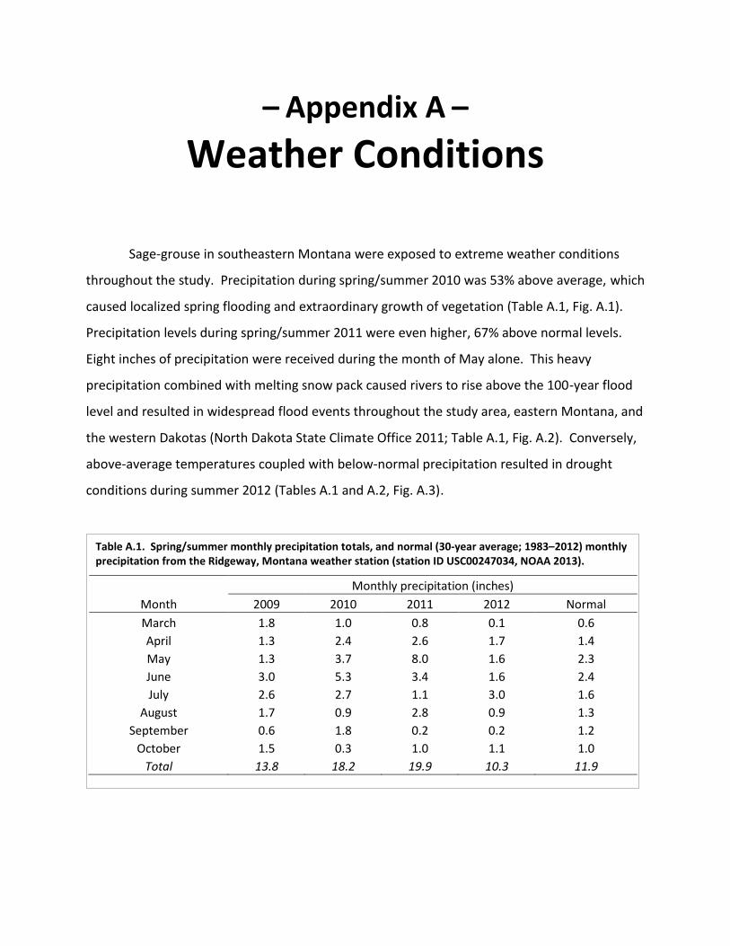
– Appendix A –

Weather Conditions

Sage-grouse in southeastern Montana were exposed to extreme weather conditions

throughout the study. Precipitation during spring/summer 2010 was 53% above average, which

caused localized spring flooding and extraordinary growth of vegetation (Table A.1, Fig. A.1).

Precipitation levels during spring/summer 2011 were even higher, 67% above normal levels.

Eight inches of precipitation were received during the month of May alone. This heavy

precipitation combined with melting snow pack caused rivers to rise above the 100-year flood

level and resulted in widespread flood events throughout the study area, eastern Montana, and

the western Dakotas (North Dakota State Climate Office 2011; Table A.1, Fig. A.2). Conversely,

above-average temperatures coupled with below-normal precipitation resulted in drought

conditions during summer 2012 (Tables A.1 and A.2, Fig. A.3).

Table A.1. Spring/summer monthly precipitation totals, and normal (30-year average; 1983–2012) monthly precipitation from the Ridgeway, Montana weather station (station ID USC00247034, NOAA 2013).

Monthly precipitation (inches)

Month 2009 2010 2011 2012 Normal

March 1.8 1.0 0.8 0.1 0.6

April 1.3 2.4 2.6 1.7 1.4

May 1.3 3.7 8.0 1.6 2.3

June 3.0 5.3 3.4 1.6 2.4

July 2.6 2.7 1.1 3.0 1.6

August 1.7 0.9 2.8 0.9 1.3

September 0.6 1.8 0.2 0.2 1.2

October 1.5 0.3 1.0 1.1 1.0

Total 13.8 18.2 19.9 10.3 11.9

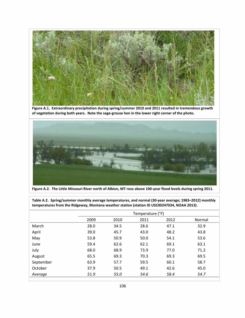
106

Table A.2. Spring/summer monthly average temperatures, and normal (30-year average; 1983–2012) monthly temperatures from the Ridgeway, Montana weather station (station ID USC00247034, NOAA 2013).

Temperature (°F)

2009 2010 2011 2012 Normal

March 28.0 34.5 28.6 47.1 32.9

April 39.0 45.7 43.0 48.2 43.8

May 53.8 50.9 50.0 54.1 53.6

June 59.4 62.6 62.1 69.1 63.1

July 68.0 68.9 73.9 77.0 71.2

August 65.5 69.3 70.3 69.3 69.5

September 63.9 57.7 59.5 60.1 58.7

October 37.9 50.5 49.1 42.6 45.0

Average 51.9 55.0 54.6 58.4 54.7

Figure A.2. The Little Missouri River north of Albion, MT rose above 100-year flood levels during spring 2011.

Figure A.1. Extraordinary precipitation during spring/summer 2010 and 2011 resulted in tremendous growth of vegetation during both years. Note the sage-grouse hen in the lower right corner of the photo.

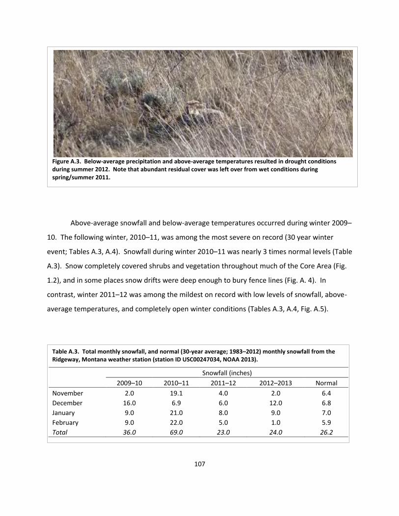
107

Above-average snowfall and below-average temperatures occurred during winter 2009–

10. The following winter, 2010–11, was among the most severe on record (30 year winter

event; Tables A.3, A.4). Snowfall during winter 2010–11 was nearly 3 times normal levels (Table

A.3). Snow completely covered shrubs and vegetation throughout much of the Core Area (Fig.

1.2), and in some places snow drifts were deep enough to bury fence lines (Fig. A. 4). In

contrast, winter 2011–12 was among the mildest on record with low levels of snowfall, above-

average temperatures, and completely open winter conditions (Tables A.3, A.4, Fig. A.5).

Table A.3. Total monthly snowfall, and normal (30-year average; 1983–2012) monthly snowfall from the Ridgeway, Montana weather station (station ID USC00247034, NOAA 2013).

Snowfall (inches)

2009–10 2010–11 2011–12 2012–2013 Normal

November 2.0 19.1 4.0 2.0 6.4

December 16.0 6.9 6.0 12.0 6.8

January 9.0 21.0 8.0 9.0 7.0

February 9.0 22.0 5.0 1.0 5.9

Total 36.0 69.0 23.0 24.0 26.2

Figure A.3. Below-average precipitation and above-average temperatures resulted in drought conditions during summer 2012. Note that abundant residual cover was left over from wet conditions during spring/summer 2011.

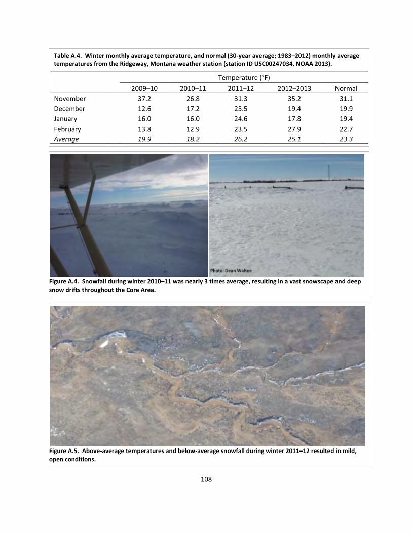
108

Figure A.5. Above-average temperatures and below-average snowfall during winter 2011–12 resulted in mild, open conditions.

Figure A.4. Snowfall during winter 2010–11 was nearly 3 times average, resulting in a vast snowscape and deep snow drifts throughout the Core Area.

Table A.4. Winter monthly average temperature, and normal (30-year average; 1983–2012) monthly average temperatures from the Ridgeway, Montana weather station (station ID USC00247034, NOAA 2013).

Temperature (°F)

2009–10 2010–11 2011–12 2012–2013 Normal

November

37.2 26.8 31.3 35.2 31.1

December

12.6 17.2 25.5 19.4 19.9

January

16.0 16.0 24.6 17.8 19.4

February

13.8 12.9 23.5 27.9 22.7

Average

19.9 18.2 26.2 25.1 23.3