Grossman’s Missing Health Threshold TITUS GALAMA, ARIE KAPTEYN

WR-684

May 2009

This paper series made possible by the NIA funded RAND Center for the Study of Aging (P30AG012815) and the NICHD funded RAND Population Research Center (R24HD050906).

WORK ING P A P E R

This product is part of the RAND Labor and Population working paper series. RAND working papers are intended to share researchers’ latest findings and to solicit informal peer review. They have been approved for circulation by RAND Labor and Population but have not been formally edited or peer reviewed. Unless otherwise indicated, working papers can be quoted and cited without permission of the author, provided the source is clearly referred to as a working paper. RAND’s publications do not necessarily reflect the opinions of its research clients and sponsors.

is a registered trademark.

GROSSMAN’S MISSING HEALTH THRESHOLD

Titus J. Galama∗ Arie Kapteyn∗

May 5, 2009

Abstract

We present a generalized solution to Grossman’s model of health capital (1972),relaxing the widely used assumption that individuals can adjust their health stockinstantaneously to an “optimal” level without adjustment costs. The Grossman modelthen predicts the existence of a health threshold above which individuals do notdemand medical care. Our generalized solution addresses a significant criticism: themodel’s prediction that health and medical care are positively related is consistentlyrejected by the data. We suggest structural and reduced form equations to test ourgeneralized solution and contrast the predictions of the model with the empiricalliterature.

Keywords: health, demand for health, health capital, medical care, labor

JEL Codes : I10, I12, J00, J24

∗RAND Corporation; This research was supported by the National Institute on Aging, under grants R01AG030824,P30AG012815 and P01AG022481. We are grateful to Arthur van Soest, Eddy van Doorslaer, Hans van Kippersluis,Erik Meijer, Raquel Fonseca, Pierre-Carl Michaud and James Hosek for useful discussions and comments.

1

1 Introduction

Grossman’s model of health capital (1972a, 1972b, 2000) is considered a breakthrough in theeconomics of the derived demand for medical care. In Grossman’s human capital frameworkindividuals demand medical care (e.g., invest time and consume medical goods and services)for the consumption benefits (health provides utility) as well as production benefits (healthyindividuals have greater earnings) that good health provides. The model has been employedwidely to explore a variety of phenomena related to health, medical care, inequality in health, therelationship between health and socioeconomic status, occupational choice, etc (e.g., Muurinenand Le Grand, 1985; Case and Deaton 2005; Cropper 1977).

Yet the Grossman model has also received significant criticism. For example, the model hasbeen criticized for its simplistic deterministic nature (e.g., Cropper 1977, Dardanoni and Wagstaff

1987), for not determining length of life (e.g., Ehrlich and Chuma, 1990), for allowing completehealth repair (Case and Deaton 2005), and for its formulation in which medical investment inhealth has constant returns which is argued to lead to an unrealistic “bang-bang” solution (e.g.,Ehrlich and Chuma, 1990). The criticism has led to theoretical and empirical extensions of themodel (often by the same authors who provided the criticism), which to a large extent address theissues identified.1 For an extensive review see Grossman (2000) and the work referenced therein.

However, there is one most significant criticism that thus far has not satisfactorily beenaddressed. Zweifel and Breyer (1997; p. 62) reject the Grossman model’s central propositionthat the demand for medical care is derived from the demand for good health: “ ... the notion thatexpenditure on medical care constitutes a demand derived from an underlying demand for healthcannot be upheld because health status and demand for medical care are negatively rather thanpositively related ...” In a review of the empirical literature Zweifel and Breyer conclude that themodel’s prediction that health and medical care should be positively related (healthy individualsconsume more medical goods and services) is consistently rejected by the data. For example,Cochrane et al. (1978) find in a study of various determinants of mortality across various countriesthat indicators of medical care usage are positively related to mortality. And more specifically,Wagstaff (1986) and Leu and Gerfin (1992), in estimating structural and reduced form equationsof the Grossman model, find that measures of medical care are negatively correlated with measuresof health and that the relationships are highly significant.2

It is of importance that this criticism be addressed. Dismissal of the central proposition ofthe Grossman model essentially amounts to rejecting the model itself. And a model of health andmedical care should at a minimum predict the correct sign of the relationship between the two.

Several authors have sought to explain the consistently negative relation between health and

1With the exception perhaps of the “bang-bang” solution and for allowing complete health repair, which we willdiscuss briefly in this work.

2Numerous other studies do not specifically test Grossman’s structural and reduced form equations, but broadly testsimilar relations between measures of health and measures for the demand for medical goods and services, controllingfor relevant demographic and other characteristics. These studies find similar results. See section 4 for a discussion.

2

medical care in empirical studies. For example, Grossman argues that the observed negativerelation could be attributed to biases that arise if the conditional demand function is estimatedwith health treated as exogenous (Grossman 2000; p. 386).

Muurinen and Le Grand (1985), in attempting to explain the positive relation betweenmortality and medical care usage found by Cochrane et al. (1978), suggest that the negativerelation between indicators of health and of medical care (apart from suggesting that medicalcare is actually harmful) could be explained by differences in socioeconomic status. Individualswith fewer resources derive relatively higher production benefits from their health stock. Theythus would have relatively greater usage of the stock (i.e., higher rates of health deterioration)which would require higher medical care to compensate for health losses. But if health cannot becompletely repaired due to the increased use-intensity they would have inferior health states. Highmortality would then be positively correlated with use of health services.

Wagstaff (1986) provides a detailed discussion of potential reasons why estimates of theGrossman model may lead to a negative relation between measures of medical care usage andmeasures of health. On the one hand, one might argue that the coefficients determined in Wagstaff

(1986) and similar analyses are not reliable estimates of the model’s parameters. For example,Wagstaff suggests that in moving from the theoretical to the empirical model inappropriateassumptions may have been introduced (see Wagstaff 1986 for details). Or the identificationof medical care with market inputs may insufficiently characterize health inputs if non-medicalinputs are important in the production of health. On the other hand, one may take the estimatesat face value and seek explanations in terms of the underlying model. Interestingly, Wagstaff

(1986) suggests that, contrary to what is assumed in Grossman’s theoretical work, the negativerelationship may reflect a non-instantaneous adjustment of health capital to its “optimal” value.3

This, Wagstaff argues, may be the result of a constraint on medical care or be due to the existenceof adjustment costs. Wagstaff finds in subsequent analysis (Wagstaff 1993) that a reformulation ofGrossman’s empirical model with non-instantaneous adjustment is not only more consistent withGrossman’s theoretical model but also with the data.

Indeed, in earlier theoretical work building on a simplified version of the Grossman model(Galama et al. 2009) we concluded that the widely employed assumption in the Grossmanliterature that any health “excess” or “deficit” can be adjusted instantaneously and at no adjustmentcost may be too restrictive. Any “excess” in health capital cannot rapidly dissipate as individualswith “excessive” health can at best decide not to consume medical care.4 As a consequence theirhealth deteriorates at the natural deterioration rate d(t) (i.e., non instantaneous) until health reachesGrossman’s “optimal” level. Thus an individual’s health is not always at the predicted “optimal”

3Throughout this paper we will refer to Grossman’s solution for the optimal health level as “optimal” health (usingquotation marks) to reflect the fact that the Grossman solution is not always the optimal solution. Grossman’s solutionis optimal only in the absence of corner solutions. In this work we explore corner solutions in which individuals do notconsume medical care for periods of time. The Grossman solution is then strictly speaking not the optimal solution.

4In other words medical care is restricted to be non-negative and the situation where individuals do consume medicalcare represents a corner solution.

3

level. While the widely employed assumption that an individual’s health follows Grossman’ssolution for the “optimal” path allows one to derive simple model predictions for empiricalvalidation (and indeed this may be the primary reason for its use), it is otherwise unnecessaryand is not demanded by theory. Importantly, Wagstaff’s (1993) work suggests that individuals donot adjust their health stocks instantaneously. In other words, not only is there no theoretical basisfor the assumption, empirical evidence suggests the assumption is not valid.

In this paper we relax the widely used assumption that individuals can adjust their health stockto Grossman’s “optimal” level instantaneously. We do not restrict an individual’s health pathto Grossman’s “optimal” solution but allow for corner solutions where the optimal response forhealthy individuals is to not consume medical goods and services for some period of time. Wethen find that the Grossman model predicts a substantially different pattern of medical care overthe life-time than previously was assumed. Healthy individuals initially do not demand medicalcare till their health has deteriorated to a certain threshold level given by Grossman’s “optimal”health. Subsequently their health evolves as the Grossman solution for the “optimal” path asindividuals begin to demand medical care. In other words, Grossman’s “optimal” health level isin fact a “health threshold” rather than an “optimal” trajectory. This simple pattern potentiallyaddresses the most damning criticism: we find that the Grossman model predicts that healthyindividuals (those above the threshold) do not consume medical care, but the unhealthy (at thethreshold) do. Grossman’s model thus predicts that healthy individuals demand less medical care,not the opposite, in agreement with the empirical literature.

Our working hypothesis is that a significant share of the population is healthy for much oftheir life. In our definition the healthy do not demand medical care. This would help explain theobserved negative relation between measures of health and measures of medical care. Further, aswe will see, this hypothesis can explain a number of other empirical facts.

A consequence of the assumption that a significant share of the population is healthy formuch of their life, combined with the threshold nature of the demand for medical care, is thathealth investment in the Grossman model is to be strictly interpreted as medical care. It isthe type of health investment (own time inputs and purchases of goods and services in themarket) that individuals engage in when they are unhealthy and seek to “repair” their health.The Grossman literature sometimes views health investment as including a wide range of othertypes of investments, such as: preventive care (e.g., medical check ups), healthy dieting, andsports / exercise. Strictly speaking, the Grossman model does not contain the concept of healthyor unhealthy consumption nor of preventive care. In contrast to medical care, individualsengage in such activities when they are healthy as well as when they are unhealthy. In otherwords, these types of health investment are not part of the current formulation of the Grossmanmodel where health investments take place only when individuals are unhealthy. The Grossmanmodel, however, does offer an alternative way to include such health investments, by slowing thedeterioration rate. For example, Case and Deaton (2005) model the effect of healthy consumption(e.g., healthy dieting, sports / exercise) as slowing and unhealthy consumption (e.g., smoking,excessive alcohol consumption) as accelerating the rate of deterioration. Preventive care may

4

operate in a similar manner. Here we consider these extensions as beyond the scope of the currentpaper.

As mentioned before, we are motivated by the lack of a theoretical justification in theGrossman literature for employing the assumption that health is always at Grossman’s “optimal”level (see Galama et al. 2009) and by Wagstaff’s (1993) empirical analysis that suggests theassumption is not valid. A further motivation comes from the observation that the above attemptsto explain the observed negative relationship between measures of health and measures of medicalcare do not pass the principle of Occam’s razor when compared to the simple explanation putforward here that individuals cannot adjust their health stocks instantaneously (Wagstaff 1986,1993; Galama et al. 2009). Our proposed explanation is the simplest in that we adopt theGrossman model as is and make one fewer assumption than is commonly made in the Grossmanliterature.

The aim of this paper is to investigate the solutions and predictions of the Grossman modelwithout restricting the solutions to Grossman’s so-called “optimal” solution by allowing forcorner solutions. We proceed as follows. In section 2, we reformulate the Grossman modelin continuous time allowing for corner solutions, solve the optimal control problem and derivefirst-order conditions for consumption and health. In section 3 we present structural form andreduced form solutions for health, medical care and consumption to enable empirical testing of ourreformulation of the Grossman model. In section 4 we contrast the predictions of our generalizedsolution of the Grossman model with the traditional solution and with the empirical literature. Weconclude in section 5 and provide detailed derivations in the Appendix.

2 General framework: the full Grossman model

We present the original human-capital model of the derived demand for health by Grossman(Grossman 1972a, 1972b, 2000) in continuous time (see also Wagstaff, 1986; Wolfe, 1985;Zweifel and Breyer, 1997; Ehrlich and Chuma, 1990). Health is treated as a form of humancapital (health capital) and individuals derive both consumption (health provides utility) andproduction benefits (health increases earnings) from it. The demand for medical care is a deriveddemand: individuals demand “good health”, not the consumption of medical care. In the originalformulation of the Grossman model (Grossman 1972a, 1972b, 2000) health yields an output ofhealthy time and consumption and medical care constitute both own-time inputs and goods orservices purchased in the market. Simplified versions of the Grossman model have been presentedby Case and Deaton (2005) who assume consumption and production benefits are functions ofhealth rather than healthy time, Wolfe (1985) who assumes health does not provide utility, andCase and Deaton (2005) and Wagstaff (1986) who do not include time inputs into the productionof consumption nor in the production of medical care. For an excellent review of the basic conceptsof the Grossman model see Muurinen and Le Grand (1985).

5

Individuals maximize the life-time utility function∫ T

0UC(t), s[H(t)]e−βtdt, (1)

where T denotes total life time, β is a subjective discount factor and individuals derive utilityUC(t), s[H(t)] from consumption C(t) and from reduced sick time s[H(t)]. Sick time is assumedto be a function of health H(t). Time t is measured from the time individuals begin employment.Utility decreases with sick time ∂U(t)/∂s(t) ≤ 0 and increases with consumption ∂U(t)/∂C(t) ≥ 0.Sick time decreases with health ∂s(t)/∂H(t) ≤ 0. Further we assume diminishing marginalbenefits: ∂2U(t)/∂2s(t) ≥ 0 and ∂2U(t)/∂2C(t) ≤ 0.

The objective function (1) is maximized subject to the following constraints:

H(t) = I(t) − d(t)H(t), (2)

A(t) = δA(t) + Ys[H(t)] − pX(t)X(t) − pm(t)m(t), (3)

and we have initial and end conditions: H(0), A(0) and A(T ) are given.H(t) and A(t) in equations (2) and (3) denote time derivatives of health H(t) and assets A(t).

Health (equation 2) can be improved through medical health investment I(t) (medical care) anddeteriorates at the “natural” health deterioration rate d(t). Using equation (2) we can write H(t) asa function of medical care I(t) and initial health H(0),

H(t) = H(0)e−

t∫0

d(s)ds+

t∫0

I(x)e−

t∫x

d(s)dsdx. (4)

Assets A(t) (equation 3) provide a return δ (the interest rate), increase with income Ys[H(t)]and decrease with purchases in the market of goods X(t) and medical goods and services m(t) atprices pX(t) and pm(t), respectively. Income Ys[H(t)] is assumed to be a decreasing function ofsick time s[H(t)].

Integrating equation (3) over the life time we obtain the life-time budget constraint

T∫0

pX(t)X(t)e−δtdt +T∫

0pm(t)m(t)e−δtdt =

A(0) − A(T )e−δT +T∫

0Ys[H(t)]e−δtdt.

(5)

The left-hand side of (5) represents life-time consumption of market goods and life-timeconsumption of medical goods and services, and the right-hand side represents life-time financialresources in terms of life-time assets and life-time earnings.

Goods X(t) purchased in the market and own time inputs τC(t) are used in the production ofconsumption C(t). Similarly medical goods and services m(t) and own time inputs τI(t) are used

6

in the production of medical care I(t). The efficiencies of production are assumed to be a functionof the consumer’s stock of knowledge E (an individual’s human capital exclusive of health capital[e.g., education]) as it is generally believed that the more educated are more efficient consumersof medical care (see, e.g., Grossman 2000),

I(t) = I[m(t), τI(t); E], (6)

C(t) = C[X(t), τC(t); E]. (7)

The total time available in any period Ω(t) is the sum of all possible uses τw(t) (work), τI(t)(medical care), τC(t) (consumption) and s[H(t)] (sick time),

Ω(t) = τw(t) + τI(t) + τC(t) + s[H(t)]. (8)

In this formulation one can interpret τC(t), the own-time input into consumption C(t) asrepresenting leisure.

Income YH[s(t)] is taken to be a function of the wage rate w(t) times the amount of timespent working τw(t),

YH[s(t)] = w(t)Ω(t) − τI(t) − τC(t) − s[H(t)]

. (9)

So far we have simply followed Grossman’s formulation in continuous time. See Wagstaff

(1986), Wolfe (1985), Zweifel and Breyer (1997), and Ehrlich and Chuma (1990) for similarformulations. Our formulation differs however in one crucial respect from prior work: weexplicitly impose the constraint that medical care is non-negative for all ages and allow for cornersolutions in which individuals do not demand medical care (I(t) = 0).

2.1 Periods where individuals do not demand medical care: I(t) = 0

It is commonly assumed that any initial “excess” in health capital can be shed and any “deficit”can be repaired over a small period of time and at negligible cost. In other words, individuals arecapable of ensuring that their health is at a certain desirable or “optimal” level (e.g., Grossman1972a, 1972b, 2000; Case and Deaton 2005; Muurinen 1982; Wagstaff 1986; Zweifel and Breyer1997, Ehrlich and Chuma 1990; Ried 1998).5 This assumption is not necessarily always statedexplicitly. The literature generally assumes that there are no corner solutions. In making thisassumption the literature restricts the solution to Grossman’s “optimal” solution. While this allowsone to derive simple model predictions for empirical validation, it is unnecessary.

It is useful to view medical health investment I(t) as encompassing activities related tohealth repair (e.g., purchases of medical goods and services and own-time inputs) and to viewhealth-damaging environments (e.g., work and living environments, etc) as affecting the rate d(t)

5While many authors realize that medical health investments cannot be negative (i.e. that corner solutions exist),the literature has not fully explored the implications of this constraint.

7

at which health capital deteriorates (see, e.g., Wagstaf 1986; Case and Deaton 2005). Similar toGrossman (1972a, 1972b, 2000) we treat the health deterioration rate d(t) as strictly exogenous.

Healthy individuals, those with health levels above the “optimal” level, may desire to substitutehealth capital for more liquid capital. In other words, individuals may wish to “sell” theirhealth. But, as equation (4) shows individuals cannot “choose” health optimally. Instead theycan consume medical care (medical health investment) I(t) optimally. But medical care I(t),viewed as health-promoting cannot be traded (individuals cannot “sell” health through negativemedical health investment) and is therefore positive for all ages I(t) ≥ 0. As a result health cannotdeteriorate faster than the health deterioration rate d(t). This corresponds to the corner solutionI(t) = 0.

Thus, we have the following optimal control problem: the objective function (1) is maximizedwith respect to the control functions C(t) and I(t) and subject to the constraints (2 and 3). TheLagrangean or generalized Hamiltonian (see, e.g., Seierstad and Sydsaeter 1987) of this problemis:

= = UC(t), s[H(t)]e−βt + qH(t)I(t) − d(t)H(t)

+ qA(t)δA(t) + Ys[H(t)] − pX(t)X(t) − pm(t)m(t) + qI(t)I(t), (10)

where qH(t) is the adjoint variable associated with the differential equation (2) for health H(t),qA(t) is the adjoint variable associated with the differential equation (3) for assets A(t), and qI(t) isa multiplier associated with the condition that health investment is non negative, I(t) ≥ 0.

2.2 First-order conditions

The first-order condition for maximization of (1) with respect to consumption, subject to theconditions (2) and (3) is (see the Appendix for details)

∂U(t)/∂C(t) = qA(0)πC(t)e(β−δ)t, (11)

where the Lagrange multiplier qA(0) is the shadow price of life-time wealth (see, e.g., Case andDeaton 2005) and πC(t) is the marginal cost of consumption C(t)

πC(t) ≡pX(t)

∂C(t)/∂X(t)=

w(t)∂C(t)/∂τC(t)

. (12)

The first-order condition for maximization of (1) with respect to health, subject to theconditions (2) and (3) is (see the Appendix for details)

∂U(t)∂s(t)

∂s(t)∂H(t)

= qA(0)πI(t)

[d(t) + δ − πI(t)

]−∂Y(t)∂s(t)

∂s(t)∂H(t)

e(β−δ)t +

[qI(t) − qI(t)d(t)

]eβt

≡ qA(0)[πH(t) − ϕH(t)

]e(β−δ)t +

[qI(t) − qI(t)d(t)

]eβt, (13)

8

where πI(t) is the marginal cost of medical health investment I(t) (see equation 10 in Grossman2000)

πI(t) ≡pm(t)

∂I(t)/∂m(t)=

w(t)∂I(t)/∂τI(t)

(14)

πI(t) ≡ π(t)/π(t), πH(t) is the user cost of health capital at the margin,

πH(t) ≡ πI(t)[d(t) + δ − πI(t)

], (15)

and ϕH(t) is the marginal production benefit of health

ϕH(t) ≡∂Y(t)∂s(t)

∂s(t)∂H(t)

. (16)

Note that we have to impose that the user cost of health capital at the margin exceeds themarginal production benefits of health πH(t) > ϕH(t). Without this condition, the consumption ofmedical care would finance itself by increasing wages by more than the user cost of health. As aresult of this, consumers would choose infinite medical care paid for by infinite earnings increasesto reach infinite health.

Equations (11) and (13) describe the first-order conditions for the constrained optimizationproblem. Equation (11) is similar to equation 4a by Wagstaff (1986) and equation 6 by Caseand Deaton (2005). Equation (13) is similar to equations 13, 1-13 and 11 of Grossman (1972a),(1972b) and (2000), respectively, equation 4b by Wagstaff (1986), equation 3.5 of Zweifel andBreyer (1997), and equation 6 by Case and Deaton (2005), for qI(t) = 0 (i.e., I(t) > 0).6 Theessential difference between our results and those of fore mentioned authors is in the term qI(t)which is non-vanishing for I(t) = 0.

2.3 Grossman’s solutions for consumption and health

The first-order condition (13) contains an expression in the multiplier qI(t) which is non-vanishing(qI(t) , 0) for corner solutions in which individuals do not demand medical care (I(t) = 0). Let’sfirst focus on the solution where qI(t) = 0. This special case corresponds to the solutions found byGrossman (1972a, 1972b, 2000). The first-order condition (13) determines the “optimal” level ofhealth for the “traditional” Grossman solution.

Denoting Grossman’s “optimal” solutions for consumption, consumption goods, medical care,medical goods and services, own time input into the production of consumption, own time inputinto the production of medical care, sick time and health by C

∗(t), X

∗(t), I

∗(t), m

∗(t), τC

∗

, τI∗

, s∗(t),

and H∗(t), we have:

∂U(t)/∂C∗(t) = qA

∗

(0)πC∗

(t)e(β−δ)t, (17)

6Various other authors have presented first-order conditions for the Grossman model. The list provided here is notexhaustive.

9

and,

∂U(t)∂s∗(t)

∂s∗(t)

∂H∗(t)

= qA∗

(0)πI∗

(t)[d(t) + δ − πI

∗

(t)]−∂Y(t)∂s∗(t)

∂s∗(t)

∂H∗(t)

e(β−δ)t

≡ qA∗

(0)[πH

∗

(t) − ϕH∗

(t)]

e(β−δ)t. (18)

The first-order condition (17) determines the level of consumption. It requires the marginalbenefit of consumption to equal the product of the shadow price of life-time wealth qA

∗

(0),the marginal cost of consumption πC

∗

(t), and a time varying exponent that either grows ordecays with time, depending on the difference β − δ between the time preference rate β and theinterest rate δ. Increasing lifetime resources will lower qA

∗

(0)7 and hence increase consumption.The marginal cost of consumption πC

∗

(t) increases with the price pX∗

(t) of consumptiongoods X

∗(t) and with wages w(t), and decreases with the efficiency of consumption goods in

producing consumption, ∂C∗(t)/∂X

∗(t) and with the efficiency of time inputs τC

∗

(t) in producingconsumption, ∂C

∗(t)/∂τC

∗

(t) (see equation 12). Since the marginal benefit of consumption∂U(t)/∂C

∗(t) is a decreasing function of consumption C

∗(t), higher prices of consumption goods

pX∗

(t), higher wages w(t) and lower efficiencies ∂C∗(t)/∂X

∗(t) and ∂C

∗(t)/∂τC

∗

(t)8 lower theequilibrium level of consumption C

∗(t).

The marginal benefit of health (equation 18) equals the product of the shadow price of life-timewealth qA

∗

(0), the user cost of health capital at the margin πH∗

(t) minus the marginal productionbenefits of health ϕH

∗

(t), and a time varying term with exponent −(β − δ)t. Since the marginalbenefit of health [∂U(t)/∂s

∗(t)][∂s

∗(t)/∂H

∗(t)] is a decreasing function in health H

∗(t), lower

lifetime resources (higher qA∗

(0)), higher user cost of health capital πH∗

(t) and lower productionbenefits of health ϕH

∗

(t) will lower the level of health H∗(t). The user cost of health capital

(see equations 14 and 15) increases with the price pm∗

(t) of medical goods/services, with wagesw(t), the health deterioration rate d(t) and the rate of return on assets δ (reflecting an opportunitycost). The user cost of health capital decreases with the efficiency of medical goods/services inproducing medical care, ∂I(t)/∂m

∗(t), the efficiency of time input τI

∗

(t) in producing medical care,∂I∗(t)/∂τI

∗

(t), and with πI∗

(t), the rate of relative change in the marginal cost of medical care πI∗

.The marginal production benefit of health ϕH

∗

(t) (equation 16) increases with the extent to whichhealth increases earnings [∂Y(t)/∂s

∗(t)][∂s

∗(t)/∂H

∗(t)].

A lower price of medical goods/services thus increases health. This is pertinent in across-country comparison, but also when comparing across the life-cycle, for instance if healthcare is subsidized for certain age groups (like Medicare in the U.S.) Also, more efficient medicalcare will lead to greater health. Efficiency can explain variations within a country (if for instanceindividuals with a higher education level are more efficient consumers of medical care, Goldmanand Smith, 2002) or across countries (if health care is more efficient in one country than inanother).

7This result can be obtained by substituting the solutions for consumption, health, and medical care in the budgetconstraint (equation 5) and solving for qA(0). See, for example, Galama et al. (2009).

8I.e., where large increases in X∗(t) and/or τC∗

(t) result in an insignificant increase in C∗(t).

10

2.4 Corner solutions

We allow for corner solutions in which individuals do not demand medical care I(t) = 0. Thissituation occurs when individuals have initial health endowments H(0) that are greater thanGrossman’s “optimal” level of health H

∗(0).

We follow a simple intuitive approach. The corner solution is associated with a non-vanishingLagrange multiplier qI(t). The solution for consumption is still provided by the first-ordercondition (11) as this condition is independent of the Lagrange multiplier qI(t). The solutionfor medical care is simply

I(t) = 0. (19)

We do not need to use the first-order condition (13) to obtain the solution for health. Usingequation (4) and I(x) = 0 we have

H(t) = H(0)e−

t∫0

d(s)ds. (20)

In other words, in the absence of medical care health deteriorates at the natural deterioration rated(t). The corner solution is fully determined by equations (11), (19) and (20).

3 Empirical model

The Grossman literature assumes that an individual’s health follows Grossman’s “optimal” healthpath, H

∗(t) (e.g., Grossman 1972a, 1972b, 2000; Case and Deaton 2005; Muurinen 1982; Wagstaff

1986; Zweifel and Breyer 1997, Ehrlich and Chuma 1990; Ried 1998). In other words, theliterature assumes that either the initial health endowment H(0) is at or very close to Grossman’s“optimal” health stock H

∗(0) or that individuals find this health level desirable and are capable of

rapidly dissipating or repairing any “excess” or “deficit” in health.Corner solutions, where individuals do not demand medical care (I(t) = 0), occur when

individuals are healthy, i.e. H(t) > H∗(t). Health then deteriorates at the natural deterioration

rate d(t) (see equation 20) until it reaches Grossman’s level H(t) = H∗(t). Individuals then

begin to demand medical care I(t) > 0. In other words, the Grossman solution for the “optimal”health stock represents a health “threshold” instead. In our generalized solution of the Grossmanmodel, H

∗(t) is the minimum health level individuals “demand” to be economically productive

(production benefits of health) or satisfied (consumption benefits of health). Individuals onlyconsume medical care when they are “unhealthy” (health levels at the threshold) and not whenthey are “healthy” (health levels above the threshold).

Wolfe (1985) assumes an initial surplus of health and is, to the best of our knowledge, theonly researcher who has attempted to explore the consequences of corner solutions in Grossman’smodel in some detail. Wolfe employs a simplified Grossman model where health (or, alternatively,reduced sick time as in Grossman’s original formulation) does not provide utility. Wolfe interprets

11

the onset of “ . . . a discontinuous mid-life increase in health investment . . . ” with retirement. Wehowever do not associate the discontinuous increase in medical health investment with retirementbut with becoming unhealthy (health levels at the health threshold leading to consumption ofmedical care to improve health). We allow the onset of medical health investment to take placeanytime during the life of individuals, including allowing for the possibility that the onset neveroccurs. While Wolfe (1985) provides a convincing argument that high initial health endowmentsare plausible9, we simply assume that initial health H(0) can take any positive value (includingvalues below the health threshold).

We distinguish three scenarios as shown in figure 1. We show the simplest case in whichthe health threshold H

∗(t) is constant across age (e.g., for constant user cost of health capital

πH∗

(t) = πH∗

(0), constant production benefits of health ϕH∗

(t) = ϕH∗

(0) and for β = δ; seeequations 17 and 18) but the scenarios are valid for more general cases. Scenarios A and B beginwith initial health H(0) greater than the initial health threshold H

∗(0) and scenario C begins with

initial health H(0) below the initial health threshold H∗(0). In scenario A health H(t) reaches the

health threshold H∗(t) during life (before the age of death T ) at age t1. In scenario B health H(t)

never reaches the health threshold H∗(t) during the life of the individual. In scenario C individuals

begin working life with health levels H(0) below the initial health threshold H∗(0).

In scenarios A and B the solution for health is determined by the corner solution presentedin section 2.4 for young ages (scenario A) or all ages (scenario B). In scenario A, after healthreaches the threshold level the solutions are determined by the “traditional” Grossman solution. Inscenarios A and B we do not have to assume that individuals adjust their health to reach the healththreshold.

In contrast, in scenario C we follow the traditional Grossman model and assume that anindividual is able to adjust his/her health level to reach the health threshold (“optimal” health).Individuals will invest initial assets A(0) to improve initial health H(0) such that initial healthequals the initial health threshold H(0) = H

∗(0). These solutions have been criticized by

Ehrlich and Chuma (1990) as being unrealistic “bang-bang” solutions; the adjustment takes placeinstantaneously. It is, however, not necessary to assume that the adjustment is instantaneous asindividuals will have had ample time to consume medical care before they enter the labor force.There is also naturally an adjustment cost associated with these medical investments in the sensethat such individuals begin their work life with fewer assets as a result of the purchase of medicalcare in the market before they entered the labor force. In other words, by the time individuals enterthe labor force their health has gradually reached the health threshold and the adjustment cost is

9On the grounds that “. . . the human species, with its goal of self-preservation, confronts a different problem thanthe individual who seeks to maximize utility. The evolutionary solution to the former may entail an excessive healthendowment in the sense that an individual might prefer to have less health and to be compensated with wealth in amore liquid form . . . ” In other words, humans may have been endowed with “excessive” health as a result of ourevolutionary history which required good physical condition to hunt and gather food, defend ourselves, survive periodsof hunger etc. Today’s demands on human’s physical condition are essentially based on the utility of good health andon economic productivity, which in an increasingly knowledge-intensive environment may be significantly smaller thanin pre-historic times.

12

reflected in reduced assets. The health of such individuals will then continue to evolve along thehealth threshold (the “optimal” health path).

Further, as mentioned before, our working hypothesis is that most individuals are healthy formost of their life (health levels above the health threshold). A consequence of this is that scenarioC, where initial health is below the initial health threshold, is less relevant for our discussion.That is, we do not disagree with Ehrlich and Chumas criticism of the Grossman model. Theformulation could benefit from a more realistic incorporation of medical technology (allowed toinstantaneously take effect in the Grossman model) or from diminishing returns to medical careso that a consumer doesn’t demand such investment all at once (the solution Ehrlich and Chumaoffer; see also Case and Deaton, 2005). For the purpose of the current research such extensionswould complicate the model and provide relatively little benefit.

Figure 1: Three scenarios for the evolution of health. t1 in scenario A denotes the age at whichhealth (solid line) has evolved towards the threshold health level (dotted line).

Following Grossman (1972a, 1972b, 2000) and Wagstaff (1986) we derive structural andreduced form equations for empirical testing. Empirical tests of Grossman’s model in the empiricalliterature have been based on estimating two sub-models (1) the “pure investment” model in whichthe restriction [∂U(t)/∂s(t)][∂s(t)/∂H(t)] = 0 is imposed and (2) the “pure consumption” modelin which the restriction [∂Y(t)/∂s(t)][∂s(t)/∂H(t)] = 0 is imposed. To allow comparison withprevious research we adopt the same restrictions and explore the same two sub-models. AsWagstaff (1986) notes equation (18) can be transformed into a linear estimating equation withthe restriction [∂U(t)/∂s(t)][∂s(t)/∂H(t)] = 0 or [∂Y(t)/∂s(t)][∂s(t)/∂H(t)] = 0, but this is notthe case for the more general model. In addition, without imposing these restrictions analyticalsolutions for health, medical care and consumption cannot be obtained without making furtherassumptions. Lastly, the two sub models represent two essential characteristics of health: healthas a means to produce (investment) and health as a means to provide utility (consumption). Wenow discuss each sub-model in turn.

13

3.1 Pure investment model

In the following we follow Grossman (1972a, 1972b, 2000). We impose

[∂U(t)/∂s(t)][∂s(t)/∂H(t)] = 0, (21)

assume that sick time is a power law in health

s(t) = β0 + β1H(t)−β2 , (22)

where β1 and β2 are positive constants (e.g., Wagstaff 1986).10 We thus have[∂Y(t)/∂s(t)][∂s(t)/∂H(t)] = β1β2w(t)H(t)−(β2+1). We further assume that medical healthinvestment (medical care) is produced by combining own time and medical goods/servicesaccording to a Cobb-Douglass constant returns to scale production function

I(t) = µI(t)m(t)1−kIτI(t)kI eρI E , (23)

where µI(t) is an efficiency factor, 1 − kI is the elasticity of medical care I(t) with respect tomedical goods/services m(t), kI is the elasticity of medical care I(t) with respect to health timeinput τI(t), and ρI determines the extent to which education E improves the efficiency of medicalcare I(t). Further, the ratio of the marginal product of medical care with respect to medicalgoods/services ∂I(t)/∂m(t) and the marginal product of medical care with respect to own timeinvestment ∂I(t)/∂τI(t) equals the ratio of the price of medical goods/services pm(t) to the wagerate w(t) (representing the opportunity cost of time; see equation 14)

∂I(t)/∂m(t)∂I(t)/∂τI(t)

=pm(t)w(t)

=1 − kI

kI

τI(t)m(t)

. (24)

Lastly, we follow Wagstaff (1986) and Cropper (1981) and assume the health deterioration rated(t) to be of the form

d(t) = d•eβ3t+β4X(t), (25)

where d•≡ d(0)e−β4X(0) and X(t) is a vector of environmental variables (e.g., working and living

conditions, hazardous environment, etc) that affect the deterioration rate. The vector X(t) mayinclude other exogenous variables that affect the deterioration rate, such as education (Muurinen,1982).

3.1.1 Health threshold

Structural form equations The structural form equation for the health “threshold” (Grossman’ssolution for “optimal” health) is as follows (see the Appendix for details)

lnH(t) = β5 + ε(1 − kI)lnw(t) − ε(1 − kI)lnpm(t) + ερIE − ε(β3 + β6)t − εβ4X(t)

− ε ln d•− ε ln1 + d−1

•e−β3t−β4X(t)[δ − kIw(t) − (1 − kI) pm(t) − β6], (26)

10But note that negative values can be allowed as long as β1β2 > 0

14

where ε ≡ (β2 + 1)−1, the constant β5 ≡ ε ln(β1β2) + ε ln[kkII (1 − kI)

(1−kI )] + ε ln µI(0), and weallow medical technology µI(t) = µI(0)e−β6t to depend on age (e.g., the efficiency of medicalgoods/services m(t) and own time inputs τI(t) in improving health could diminish with age).11 Itis customary to assume that the term ln d

•in equation (26) is an error term with zero mean and

constant variance ξ1(t) ≡ − ln d•

(as in Wagstaff, 1986, and Grossman 1972a, 1972b, 2000) andthat the term ln[1 + δ/d(t)− πI(t)/d(t)] (the last term in equation 26) is small or constant (see, e.g.,Grossman 1972a, 2000),12 or that it is time dependent ln[1+δ/d(t)− πI(t)/d(t)] ∝ t (e.g, Wagstaff,1986). We do not have to make these assumptions as in our generalized solution of the Grossmanmodel the rate of deterioration d(t) is observable for those times that individuals do not demandmedical care (i.e., for corner solutions). While we assume that the last term in equation (26) issmall, our formulation allows us to estimate and test this common assumption.

The demand for health (equation 26) thus increases with wages w(t) and with education Eand decreases with prices pm(t) and the health deterioration rate (terms d

•, β3 and β4X(t)). The

relation with age t is ambiguous. To ensure that health declines with age, it is commonly assumedthat health deterioration increases with age, d(t) > 0 (i.e. that β3 > 0).13 But since wagesw(t) generally increase with years of experience (e.g., Mincer 1974) it is possible that the healththreshold initially increases with age t.

The structural equation for the “optimal” consumption of medical goods/services is as follows

lnm(t) = β7 + ln H(t) + kIlnw(t) − kIlnpm(t) − ρIE

+ (β3 + β6)t + β4X(t) + ln d•

+ ln[1 + H(t)d−1•

e−β3t−β4X(t)], (27)

where β7 ≡ − ln µI(0) − kI ln[kI/(1 − kI)

]. It is customary to assume that the last term in

equation (27), ln[1+H(t)/d(t)] = ln[1+H(t)d−1•

e−β3t−β4X(t)], is small and can be ignored (Grossman1972b) or treated as an error term (Wagstaff 1986). This would require that the effective rate ofchange in health H(t) is smaller than d(t)H(t). This assumption is perhaps not unreasonable ifmedical care is efficient and slows down the effective health decline H(t). Note, once more that inour generalized solution of the Grossman model d(t) can be observed during times when cornersolutions hold. The last term in equation (27) can thus be estimated. For small H(t)/d(t), we haveln[1 + H(t)/d(t)] ∼ H(t)/d(t).

Equation (27) predicts that Grossman’s “optimal” demand for medical goods/services andGrossman’s “optimal” demand for health are positively related. This is the crucial prediction

11For example, elderly and frail patients may not be able to cope with certain aggressive chemotherapy regiments.Note also that advances in medical technology could be modeled by an increasing µI(0) with time (e.g., µI(0) increaseswith subsequent cohorts).

12This would require that the real interest rate δ and changes in the ratio of the price of medical goods/services andthe efficiency of medical goods/services in producing medical care πI(t) = pm(t)/[∂I(t)/∂m(t)] are much smaller thanthe health deterioration rate d(t) or that changes in the interest rate and in πI(t) follow the same pattern as changes ind(t) (so that the term is approximately constant).

13Assuming that the efficiency of medical care decreases with age β6 > 0 provides an alternative means to achievethe same result.

15

which empirical studies consistently reject. Further, the demand for medical goods/servicesincreases with wages w(t) and the health deterioration rate (terms d

•, β3 and β4X(t)), and decreases

with education E and prices pm(t).The literature usually focuses on the equations for health (26) and medical care (27), but note

that equation (11) provides a condition for consumption C(t) as well, which, after making somereasonable assumptions, can be utilized to obtain expressions for consumption goods X(t) (see theAppendix for details). The budget constraint (equation 5) then provides the solution for assetsA(t).

Reduced form equations Wagstaff (1986) notes that one way of overcoming the unobservabilityof health capital is to estimate reduced-from demand functions for health and medicalgoods/services. Combining (26) and (27) and eliminating any expression in health H(t) we find(see the Appendix for details):

ln m(t) = β8 + [kI + ε(1 − kI)]lnw(t) − [kI + ε(1 − kI)]lnpm(t)

− (1 − ε)ρIE − ε[β3 − (1 − ε)β6]t − εβ4X(t) − ε ln d•

− ε ln1 + d−1•

e−β3t−β4X(t)[δ − kIw(t) − (1 − kI) pm(t) − β6]

+ lnε(1 − kI)[w(t) − pm(t)] − ε(β3 + β6) − εβ4∂X(t)/∂t + d•eβ3t+β4X(t) + εO(t), (28)

where β8 ≡ β5 + β7 and

O(t) =d(t)[δ − kIw(t) − (1 − kI) pm(t) − β6] + kI[

w(t)w(t) − w(t)2] + (1 − kI)[

pm(t)pm(t) − pm(t)2]

[d(t) + δ − kIw(t) − (1 − kI) pm(t) − β6],(29)

which we assume to be small (of the order d(t) × δ, d(t) × w(t), etc).The demand for medical goods/services (equation 28) increases with wages w(t) and the

efficiency of medical care (term β6), and decreases with prices pm(t), education E, and the healthdeterioration rate (terms d

•, β3 and β4X(t)).14

3.1.2 Corner solution

We have (using equations 20 and 25)

ln H(t) = ln H(0) − d•

∫ t

0eβ3 s+β4X(s)ds, (30)

andm(t) = 0. (31)

Note that during periods in which the corner solutions hold it is in principle possible to determinethe rate of deterioration d

•empirically. Hence we do not have to assume that the term ln d

•in

equations (26) and (27) is an error term.14For 0 < ε < 1.

16

3.1.3 Regime switching

The time t1 when health has deteriorated to the “threshold” level must satisfy the followingcondition (given by equating 26 with 30):

lnH(t1) = β5 + ε(1 − kI)lnw(t1) − ε(1 − kI)lnpm(t1) + ερIE − ε(β3 + β6)t1 − εβ4X(t1)

− ε ln d•− ε ln1 + d−1

•e−β3t1−β4X(t1)[δ − kIw(t1) − (1 − kI) pm(t1) − β6]

= ln H(0) − d•

∫ t1

0eβ3 s+β4X(s)ds (32)

The model thus implies a switch of regimes at time t1. Before t1 the evolution of health isgiven by equation (30), whereas after t1 it is given by (26). Empirically, this would generate aswitching regression model with endogenous switching. Once health hits the “optimal” path, theprocess governing health switches from (30) to (26). Similarly, before t1 the demand for medicalgoods/services is given by equation (31), whereas after t1 it is given by (27) or, alternatively, by(28).

3.2 Pure consumption model

In the following we follow Wagstaff (1986). We impose

[∂Y(t)/∂s(t)][∂[s(t)/∂H(t)] = 0. (33)

To convert (18) into estimable equations we have to specify a functional form for the utilityfunction.

3.2.1 Utility specification

Grossman (1972a, 1972b, 2000) formulates his model in terms of sick time15 and assumes thatsick time s(t) is a function of health H(t); s(t) = s[H(t)]. An alternative formulation is providedby Case and Deaton (2005). Case and Deaton formulate a simplified Grossman model in whichutility and income are functions of health H(t) directly, rather than indirectly through sick-times(t) which in turn is assumed to be a function of health s(t) = s[H(t)] (as in Grossman 1972a,1972b, 2000). Following Case and Deaton we write utility UC(t), s[H(t)] = U[C(t),H(t)] andincome Ys[H(t)] = Y[H(t)] as functions of health H(t) instead of sick time s(t). Essentially bothformulations are equivalent except that Case and Deaton’s formulation is more general, allowingfor example for earnings to be influenced not only by reductions in sick time but also increasedworker efficiency resulting from good health. And, at any time we can revert back to the originalspecification in terms of sick time if deemed desirable.

15One possible reason for this formulation is that the NORC data set the author employed in empirical testing of themodel contained information on sick days

17

We begin by noting that (see the first-order conditions 11 and 13)

∂U(t)∂H(t)

= πC(t)−1[πH(t) − ϕH(t)

] ∂U(t)∂C(t)

+[qI(t) − qI(t)d(t)

]eβt. (34)

In other words, the marginal benefit of health ∂U(t)/∂H(t) is given by the function πC(t)−1[πH(t)−ϕH(t)] times the marginal benefit of consumption ∂U(t)/∂C(t) and an additional expression inqI(t). For Grossman’s solutions we have qI(t) = 0 and the additional term vanishes.

Equation (34) suggests that the marginal utility of health ∂U(t)/∂H(t) and the marginal utilityof consumption ∂U(t)/∂C(t) are functions of both health H(t) and consumption C(t). To allow forthis we specify the following constant relative risk aversion (CRRA) utility function:

U[C(t),H(t)] =1

1 − ρ

[C(t)ζH(t)1−ζ

]1−ρ, (35)

where ζ (0 ≤ ζ ≤ 1) is the relative “share” of consumption versus health and ρ (ρ > 0) thecoefficient of relative risk aversion.

The functional form for the utility function can account for the observation that the marginalutility of consumption declines as health deteriorates (e.g., Finkelstein, Luttmer and Notowidigdo,2008). The authors find that a one-standard deviation increase in the number of chronic diseasesis associated with an 11 percent decline in the marginal utility of consumption relative tothis marginal utility when the individual has no chronic diseases (the 95 percent confidenceinterval ranges between 2 percent and 17 percent). This would rule out the strongly separablefunctional form for the utility function employed by Wagstaff (1986), where the marginal utility ofconsumption is independent of health. While we follow Wagstaff (1986) in most of the derivationswe do not adopt his utility specification.

3.2.2 Health threshold

Structural form equations The structural equation for the health “threshold” (Grossman’ssolution for “optimal” health) is as follows (see the Appendix for details)

lnH(t) = β9 + ln X(t) + ln pX(t) − kI ln w(t) − (1 − kI) ln pm(t)

+ ρIE − (β3 + β6)t − β4X(t) − ln d•

− ln1 + d−1•

e−β3t−β4X(t)[δ − kIw(t) − (1 − kI) pm(t) − β6], (36)

where β9 ≡ ln µI(0) − ln(1 − kC) + ln[kkII (1 − kI)

(1−kI )] + ln[(1 − ζ)/ζ]. The health threshold thusincreases with consumption goods X(t), prices for consumption goods pX(t), and education E anddecreases with wages w(t), prices of medical goods/services pm(t), and the health deteriorationrate (terms d

•, β3 and β4X(t)). The last term is generally assumed to be small and can be estimated

in our formulation.

18

The structural form equation for medical goods/services is the same as for the pure investmentmodel (equation 27) and is repeated for convenience:

lnm(t) = β7 + ln H(t) + kIlnw(t) − kIlnpm(t) − ρIE

+ (β3 + β6)t + β4X(t) + ln d•

+ ln[1 + H(t)d−1•

e−β3t−β4X(t)], (37)

where β7 ≡ − ln µI(0) − kI ln[kI/(1 − kI)

].

Combining equation (36) with (37) and eliminating any expression in health H(t) we find (seethe Appendix for details):

lnm(t) = β12 + ln X(t) + ln pX(t) − ln pm(t) − ln d•− β3t − β4X(t)

− ln1 + d−1•

e−β3t−β4X(t)[δ − kIw(t) − (1 − kI) pm(t) − β6]

+ lnd•eβ3t+β4X(t) − (1 − kI) pm(t) − kIw(t) − (β3 + β6) − β4∂X(t)/∂t

+ X(t) + pX(t) + O(t), (38)

where β12 ≡ β7 + β9, and the expression for O(t) is provided by equation (29).

Reduced form equations Note that the health threshold (equation 36) is expressed directly asa function of consumption goods X(t). This relation is different from the one found by Wagstaff

(1986; his equation 12), which is the result of our choice for the functional form of the utilityfunction (equation 35). Wagstaff (1986) finds that health H(t) is a function of the shadow priceof life-time wealth qA(0). We can obtain a similar reduced form expression to the one found byWagstaff (1986) by using the first-order condition (11) and making some reasonable assumptionsto obtain an expression for consumption good X(t). We then find (see the Appendix for details):

lnH(t) = β10 − χ(1/ρχ − 1)(1 − kC) ln pX(t) − χ(1 − kI) ln pm(t)

− χ[kI + (1/ρχ − 1)kC] ln w(t) + χ[ρI + (1/ρχ − 1)ρC]E

− χ[(β3 + β6) + (1/ρχ − 1)β11 + (β − δ)/ρχ]t − χβ4X(t) − χ ln d•

+ ln qA(0)−1/ρ

− χ ln1 + d−1•

e−β3t−β4X(t)[δ − kIw(t) − (1 − kI) pm(t) − β6], (39)

where

β10 ≡ χ ln µI(0) + χ(1/ρχ − 1) ln µC(0) + χ ln[kkII (1 − kI)

(1−kI )]

+ χ(1/ρχ − 1) ln[kkCC (1 − kC)(1−kC)] + χ ln[(1 − ζ)/ζ] + ln ζ1/ρ,

andχ ≡

1 + ρζ − ζ

ρ, (40)

and we allow the efficiency of consumption to depend on age µC(t) = µC(0)e−β11t.An expression for the shadow price of life-time wealth qA(0) in equation (39) can be obtained

by using the life-time budget constraint (equation 5), substituting the solutions for consumption,

19

health, and medical care and solving for qA(0) (see, for example, Galama et al. 2009). The shadowprice of life-time wealth qA(0) is found to be a complicated function of life-time wealth (assets,life-time income), wages w(t), prices pm(t), pX(t), education E and the health deterioration rate(terms d

•, β3 and β4X(t)). Wagstaff (1986) provides a simple approximation for the shadow price

of life-time wealth qA(0) (his equations 15 and 16) which may be easier to use in empirical testingof the model.

Assuming that both medical goods / services m(t) and time input τI(t) increase medical caresuggests 0 ≤ kI ≤ 1, and if education E increases the efficiency of medical care then ρI > 0 (seeequation 23). Similarly we have 0 ≤ kC ≤ 1 and ρC > 0 (see equation 62). Finkelstein, Luttmerand Notowidigdo (2008) provide evidence that the marginal utility of consumption declines ashealth deteriorates. Assuming further diminishing marginal benefits of health ∂2U(t)/∂2H(t) < 0we find 1 < χ < 1 + 1/ρ (and hence 0 < ρ < 1 and 1/ρχ > 1).

For these parameter values we find that the health threshold (equation 39) increases witheducation E, life-time wealth qA(0)−1/ρ, and decreases with the price of consumption goods pX(t),the price of medical care pm(t), wages w(t), and the health deterioration rate (terms d

•, β3 and

β4X(t)). The health threshold could increase or decrease with age depending on the sign ofχ(β3 +β6)+χ(1/ρχ−1)β11 +[(β−δ)/ρ] and on the evolution of wages w(t) with years of experience(e.g., Mincer, 1974).

Combining equation (37) with (39) we find:

lnm(t) = β13 − χ(1/ρχ − 1)(1 − kC) ln pX(t) − [kI + χ(1 − kI)] ln pm(t)

− χ[(1 − 1/χ)kI + (1/ρχ − 1)kC] ln w(t) + χ[(1 − 1/χ)ρI + (1/ρχ − 1)ρC]E

− χ[(1 − 1/χ)(β3 + β6) + (1/ρχ − 1)β11 + (β − δ)/ρχ]t

− (χ − 1)β4X(t) − (χ − 1) ln d•

+ ln qA(0)−1/ρ

− χ ln1 + d−1•

e−β3t−β4X(t)[δ − kIw(t) − (1 − kI) pm(t) − β6], (41)

where β13 ≡ β7 + β10. The demand for medical goods/services (equation 41) increases witheducation E, life-time wealth qA(0)−1/ρ, and decreases with the price of consumption goods pX(t),the price of medical goods/services pm(t), wages w(t), and the health deterioration rate (terms d

•,

β3 and β4X(t)). The health threshold could increase or decrease with age depending on the sign ofχ(1 − 1/χ)(β3 + β6) + χ(1/ρχ − 1)β11 + [(β − δ)/ρ] and on the evolution of wages w(t) with yearsof experience (e.g., Mincer, 1974).

3.2.3 Corner solution

The solutions are given by the corner solutions (30) and (31) derived in section 2.4.

20

3.2.4 Regime switching

The time t1 when health has deteriorated to the “threshold” level must satisfy the followingcondition (given by equating 36 or 39 with 30):

lnH(t1) = β9 + ln X(t1) + ln pX(t1) − kI ln w(t1) − (1 − kI) ln pm(t1)

+ ρIE − (β3 + β6)t1 − β4X(t1) − ln d•

− ln1 + d−1•

e−β3t1−β4X(t1)[δ − kIw(t1) − (1 − kI) pm(t1) − β6]

= β10 − χ(1/ρχ − 1)(1 − kC) ln pX(t1) − χ(1 − kI) ln pm(t1)

− χ[kI + (1/ρχ − 1)kC] ln w(t1) + χ[ρI + (1/ρχ − 1)ρC]E

− χ[(β3 + β6) + (1/ρχ − 1)β11 + (β − δ)/ρχ]t1 − χβ4X(t1) − χ ln d•

+ ln qA(0)−1/ρ

− χ ln1 + d−1•

e−β3t1−β4X(t1)[δ − kIw(t1) − (1 − kI) pm(t1) − β6]

= ln H(0) − d•

∫ t1

0eβ3 s+β4X(s)ds. (42)

Similar to the previous discussion for the pure investment model, the model thus implies aswitch of regimes at time t1. Before t1 the evolution of health is given by equation (30), whereasafter t1 it is given by (36) or by (39). Empirically, this would generate a switching regressionmodel with endogenous switching. Once health hits the optimal path, the process governing healthswitches from (30) to (36), or alternatively to (39). Similarly, before t1 medical care is given byequation (31), whereas after t1 it is given by (37) or alternatively (38) or (41).

4 Model Predictions

The Grossman model has been tested in a number of empirical studies on a variety of datasetsfrom different countries (Grossman 1972a; Wagstaff 1986, 1993; Leu and Doppman 1986; Leuand Gerfin 1992; van Doorslaer 1987; Van de Ven and van der Gaag, 1982; Erbsland, Riedand Ulrich 2002; Gerdtham et al. 1999; Gerdtham and Johannesson 1999).16 Despite the large

16Grossman (1972a) employs the 1963 health interview survey conducted by the National Opinion ResearchCenter (NORC) of the U.S. civilian noninstitutionalized population. Grossman employs measures of sick time andself-reported health and restricts the dataset to individuals with positive sick time. Wagstaff (1986) employs the 1976Danish Welfare Survey (DWS) and uses principal components analysis (PCA) to derive a smaller number of healthcomponents from a long list of health indicators. Wagstaff also uses the wealth of DWS measures of work environmentand use-related health depreciation. Measures of medical care employed are general practitioner visits, weeks inhospital and number of complaints for which medicine are taken. Wagstaff (1993) employs the Danish Health Survey(DHS) and uses a latent variable health model (multiple indicators multiple causes; MIMIC). Leu and Doppman (1986)employ a latent health variable, latent earnings and latent transfer income model based on Socio-medical indicators forthe population of Switzerland (SOMIPOPS) data combined with the Swiss income and wealth study (SEVS). Generalpractitioner consultations, hospital days and sick days are used as measures of medical care. Leu and Gerfin (1992)employ the same datasets as Leu and Doppman (1986) but follow a different methodology (health is a latent variable butno other latent variables are employed). Van Doorslaer (1987) estimates a latent health and latent medical knowledge

21

variety in methodologies and the diversity in cultural and institutional environments these datasetsrepresent, the studies are broadly in agreement with one another and confirm the predictions ofthe Grossman model for the demand for health. Health is found to increase with income (wages,life-time earnings), and education, and decreases with age, the price of medical goods/services,being single, and with environmental factors, such as, physically and mentally demanding workenvironments, manual labor, psychological stress factors.17

While reduced form estimates of the demand for medical care are generally in agreementwith the predictions of the Grossman model, this is not true for structural estimates (see Wagstaff

1986). Structural estimates allow for direct testing of the relationship between health (mostoften a latent health variable is employed) and medical care. The most noticeable feature ofsuch structural estimates is the consistently negative relationship between health and medical care(healthy individuals do not go to the doctor). But this relationship is predicted to be positive in thetraditional solution of the Grossman model (see equation 27; those who consume more medicalcare are healthier). Further, the negative relationship between health and medical care is foundto be the most statistically significant of any relationship between medical care and any of theindependent variables (see, e.g., Grossman 1972a; Wagstaff 1986, 1993; Leu and Doppman 1986;Leu and Gerfin 1992; van Doorslaer 1987; Van de Ven and van der Gaag, 1982; Erbsland, Riedand Ulrich 2002).

We assume that each of the scenarios A, B and C occur in reality (see Figure 1). In otherwords, that there exist healthy individuals who consume medical care during some part of their life(scenario A; initial health above the initial health threshold and the threshold reached during life),very healthy individuals who never consume medical care (scenario B; initial health well above theinitial health threshold and the threshold never reached), and ill individuals who consume medicalcare their entire life (scenario C; initial health at the health threshold). We do not a-priori knowthe distribution of healthy, very healthy and ill individuals in the population but if a statisticallysignificant share of individuals have initial health endowments H(0) above the initial healththreshold H

∗(0) (scenarios A and B) then empirical tests should be able to distinguish between

variable model to the Health Interview Survey of the Belgian National Health Research Project on Primary Health Careconducted in 1976 among the Dutch-speaking (Flemish) population. Van de Ven and van der Gaag (1982) employa MIMIC model with latent health and data from a health-care survey among 8000 households in The Netherlands.Erbsland, Ried and Ulrich (2002) use data from the German Socio Economic Panel (SOEP). They use a model with alatent health and a latent environment variable and restrict the analysis to the working population and to those with apositive demand for medical services. Gerdtham et al. (1999) use a rating scale and a time-trade off method to obtainmeasures of health as well as a self-reported measure of health from data collected in Uppsala County in Sweden.Gerdtham and Johannesson (1999) use a self-reported health measure from 1991 data of the Level of Living Survey(LNU), a random sample of the Swedish population. Both Gerdtham et al. (1999) and Gerdtham and Johannesson(1999) provide estimates of the demand for health but no structural estimates for the demand of medical care.

17In addition, these studies find that health increases with healthy behavior (sports, healthy eating and sleeping habits)and decreases with being overweight and with smoking. Females are found to be in lower health. And, moderate alcoholconsumption is found to have a positive or negligible impact on health (e.g., Gerdtham et al. 1999, Leu and Doppman1986). Since the effect of consumption (healthy and unhealthy forms) on health as well as health behaviors (exercise,sleeping habits) and gender differences are not part of the Grossman model we do not discuss these here.

22

the interpretation of the Grossman model advocated here (represented by the joint occurrences ofscenarios A, B and C) and the interpretation adopted in the literature (represented by scenario Conly).

In the following we will contrast the predictions of our interpretation of the Grossman modelwith the more generally held interpretation and with empirical observations from the literature.

4.1 Similarities

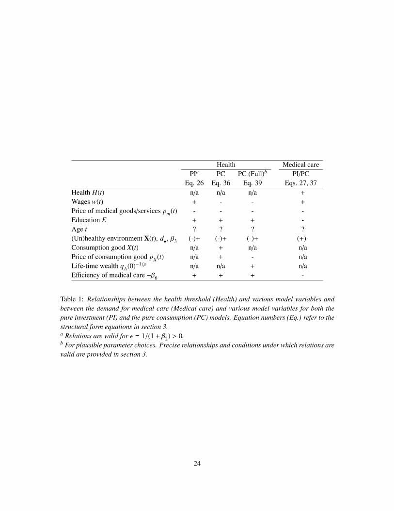
The predictions for the demand for health and for medical care for unhealthy individuals (thoseindividuals whose health is at the threshold) in our generalized solution of the Grossman modelare, with the exception of some minor differences in formulation, the same as for the originalsolution of the Grossman model. Those predictions have largely been verified in the empiricalliterature, with the exception of the relation between the demand for health and the demand formedical care (see for details the earlier discussion and references therein). We summarize ourpredictions in Table 1.

Our generalized solution of the Grossman model broadly replicates the predictions of thetraditional solution of the Grossman model. This can be seen as follows. Since the empiricalliterature has not distinguished between healthy and unhealthy individuals (a concept introducedin this work) a mixture of healthy and unhealthy individuals will have been included in the samplesinvestigated. If at any time the proportion of unhealthy individuals (those whose health is at thehealth threshold and who behave according to the traditional Grossman solution) is significant thiscould produce the observed relationships, with the exception of the relation between health andmedical care. The reason that the relationship between health and medical care is different stemsfrom the significantly different behavior between healthy and unhealthy individuals. The healthydo not consume medical care while the unhealthy do. If both healthy and unhealthy individualsare included in a sample this would produce the observed strong negative relationship betweenmeasures of health and measures of medical care. At the same time, if we can restrict the sampleto the unhealthy, we should observe the positive relationship between health and medical care aspredicted by Grossman.18

As Table 1 shows we expect health to decrease with the price of medical goods/services pm(t),unhealthy environmental factors (X(t), d

•, β3), and increase with education E19 and with the

efficiency of medical care −β6. The relation with age t is ambiguous as wages w(t) increasewith working experience (e.g., Mincer, 1974) potentially countering the “aging” variables β3, β6,

18Note that in retirement there is no production benefit from health as income, a pension / savings, is independentof the health status of the individual. Whether individuals demand less health as a result is unclear. The increasedavailability of leisure could reduce or increase the demand for health depending on whether leisure is a substitute orcompliment of health (see for a discussion Galama et al. 2009). Given potential differences in the demand for healthbetween workers and retirees it may be necessary to distinguish between workers and retirees to potentially establishthe positive relationship between health and medical care.

19Note that education could possible enter through lowering the rate of health deterioration d(t) in addition, or as analternative, to increasing the efficiency of medical care; see, e.g., Muurinen (1982)

23

Health Medical carePIa PC PC (Full)b PI/PC

Eq. 26 Eq. 36 Eq. 39 Eqs. 27, 37Health H(t) n/a n/a n/a +

Wages w(t) + - - +

Price of medical goods/services pm(t) - - - -Education E + + + -Age t ? ? ? ?(Un)healthy environment X(t), d

•, β3 (-)+ (-)+ (-)+ (+)-

Consumption good X(t) n/a + n/a n/aPrice of consumption good pX(t) n/a + - n/aLife-time wealth qA(0)−1/ρ n/a n/a + n/aEfficiency of medical care −β6 + + + -

Table 1: Relationships between the health threshold (Health) and various model variables andbetween the demand for medical care (Medical care) and various model variables for both thepure investment (PI) and the pure consumption (PC) models. Equation numbers (Eq.) refer to thestructural form equations in section 3.a Relations are valid for ε = 1/(1 + β2) > 0.b For plausible parameter choices. Precise relationships and conditions under which relations arevalid are provided in section 3.

24

β − δ. The effect of wages w(t) is unclear, with a positive effect on health in the pure investment(PI) and a negative effect on health in the pure consumption (PC) model. Do note however thatthe predictions for the PC model have less predictive power than for the PI model. The structuralform equation (36) includes consumption good X(t), an endogenous variable, which in turn is afunction of exogenous variables, such as wages w(t), the price of medical goods/services pm(t),education E, etc. The inclusion of consumption good X(t) in the structural form equation maydistort the relationships between health and the exogenous variables. While the structural formequation (39) does not suffer from this problem, the predictions shown in the table depend onassumptions about model parameters (see table note b in the Table 1). In addition, the shadowprice of life-time wealth qA(0) is a complicated function of various exogenous variables over thelife cycle. Equation (39) thus suffers from a similar lack of transparency.

With regard to the demand for medical care, Table 1 shows that we expect the demand formedical goods/services to decrease with the price of medical goods/services pm(t), education Eand the efficiency of medical care −β6, and to increase with health H(t), wages w(t) and unhealthyenvironmental factors (d

•, β3, X(t)). The predictions for the PI and PC models are the same.

As discussed earlier the positive relationship between health and medical care is expected to beobservable only if the sample can be restricted to unhealthy individuals.

4.2 Differences

In addition to the above predictions of our generalized solution of the Grossman model that arethe same as in the traditional solution of the model, there are a number of distinctly differentpredictions. Those are discussed in detail below. We denote the predictions of our interpretationof the Grossman model by Health threshold, the more generally held interpretation by “Optimal”stock and the empirical observations from the literature by Empirical literature.

1. Medical care and health are negatively correlated if measured across healthy andunhealthy individuals

“Optimal” stock: Health and medical care are positively correlated (see equations 27 and37), i.e. individuals who consume more medical care are healthier.

Health threshold: Healthy individuals (H(t) > H∗(t)) do not consume medical care, while

unhealthy individuals (H(t) = H∗(t)) do. I.e. healthy individuals do not go to the doctor

much, do not take much medicine, are not found to stay often in hospitals. Measured acrossa sample of healthy and unhealthy individuals we expect unhealthy individuals to consumemore medical care than healthy individuals.

Empirical literature: As discussed earlier the most striking feature of structural formestimates of the demand for medical care (see, e.g., Grossman 1972a; Wagstaff 1986, 1993;Leu and Doppman 1986; Leu and Gerfin 1992; van Doorslaer 1987; Van de Ven and vander Gaag 1982; Erbsland, Ried and Ulrich 2002) is the persistent and highly statisticallysignificant negative relation found between measures of health and measures of medical

25

care. The studies employ a variety of methodologies and a variety of datasets representingdifferent cultural and institutional settings in a number of different countries (Europe andU.S.), yet their findings are largely in agreement with one another. None of these studiesseparate a healthy from an unhealthy population and hence we expect to observe a strongnegative correlation between health and medical care if the population consists of bothhealthy and unhealthy individuals.20

2. Healthy people do not consume medical care

“Optimal” stock: In the standard solution of the Grossman model individuals consumemedical care at all ages.

Health threshold: In our generalized solution healthy individuals (individuals whose healthH(t) is above the threshold H

∗(t)) do not consume medical goods/services, i.e. we

would expect some fraction of the population at any given time to not consume medicalgoods/services.

Empirical literature: We would expect that healthy people pay few visits to the doctor(perhaps only to prevent illness, such as for a “health check up”) and that they do notrequire much medical care (hospital stays, use medicine, etc). For example, Wagstaff (1986)observes that 48% of the 1976 Danish Welfare Survey (DWA) sample he employed recordedzero general practitioner visits and 46.5% recorded zero weeks in hospital.

3. Effective health deterioration slows when individuals reach the health threshold

“Optimal” stock: In the standard solution of the Grossman model health evolves asGrossman’s “optimal” health stock, i.e. we do not expect to see discontinuous changesin the evolution of health.

Health threshold: Healthy people (H(t) > H∗(t)) do not consume medical goods/services

and their health deteriorates at the “natural” deterioration rate H(t) = −d(t)H(t). When, as aresult of health deterioration their health reaches the health threshold H(t) = H

∗(t) (i.e., they

have become unhealthy by our definition) they begin to consume medical goods/servicesand their health deteriorates at a lower effective rate H(t) = I(t) − d(t)H(t). If medicalcare improves one’s health (e.g., medical care is effective), we expect to observe slowereffective health deterioration H(t) or even health improvement when individuals reach thehealth threshold and begin to consume medical goods/services).21

20Grossman (1972a) however selected a sub sample of the NORC dataset by restricting the data to those individualsthat reported positive sick time and Erbsland, Ried and Ulrich (2002) restricted the sample to individuals reportingpositive demand for health services. Interestingly Grossman (1972a) shows the least statistically significant negativerelation between health and medical outlays of all the studies (t-stat of -5.84 [see table 7 OLS estimates]). Erbsland,Ried and Ulrich (2002) report t-values of around -10 for three measures of medical care usage. Other studies, on theother hand, report values of at least -10 and up to -90. Perhaps the restriction of the samples to individuals that reportpositive sick time or positive medical care partially limited the sample to unhealthy respondents.

21Note the distinction between the effective health deterioration rate H(t) and the “natural” health deterioration rated(t).

26

Empirical literature: Van Kippersluis et al. (2008) examine inequality in self-reportedhealth (SRH) as a function of income in 11 European countries. The authors transform theordinal SRH information onto a cardinal scale using utility scores for the SRH categoriestaken from the 2001 Canadian Community Household Survey (CCHS). The authors finda remarkable consistency in the pattern of health with age. In most countries healthdeteriorates gradually from early adulthood until around age 50 after which it generallylevels off before accelerating rapidly after age 70. The authors find this middle-age plateau(ages 50-70) rather puzzling, but it would be consistent with a slowing of the decline inhealth resulting from increased medical care as the average individual reaches a healththreshold. After age 70, as terminal illnesses set in, health again declines rapidly.

Smith (2004, 2007) uses self-reported health (SRH) status from the National HealthInterview Survey (NHIS) and PSID to show how disparity in health between low-and high-income individuals (the so-called socio-economic status [SES]-health gradient)increases with age till about age 60 after which the disparity narrows (see Van Doorslaeret al. 2008 for an excellent review of the literature on the SES-health gradient over the lifecycle). The percentage of individuals reporting excellent or very good health status declinesrapidly till age 60 for the first income quartile households (lowest income) and then remainsfairly constant out till age 90. The 2nd to 4th income quartiles however show a more gradualdecline.

Similarly, Case and Deaton (2005) present several plots of self-reported health (SRH) statusfrom the NHIS as a function of age. Women and men in the bottom income quartile showa rapid deterioration in SRH between ages 20 and 60 after which the SRH curve flattenssignificantly (see their figure 2). Again we see no evidence for a flattening of SRH withincreasing age for the upper income quartile (in fact we see gradually deteriorating SRHstatus). This suggests that high SES individuals reach a health threshold much later (theirSRH deteriorates slower) than low SES individuals. As a result they see no need to consumemedical goods/services even at late ages and their effective health deterioration does notslow with age.

Van Kippersluis et al. (2009) find similar results for the Netherlands using a rich datasetbased on the Health Interview Surveys and administrative data from Statistics Netherlands(CBS). The data allows the authors to study SRH as well as mortality, to disentangle theeffect of ageing from that of cohort effects and to use actual (not reported) income fromtax files. The authors find the pattern of the SES-health gradient over the life cycle in theNetherlands to be remarkably similar to that in the U.S., despite significant differences inthe two countries’ institutions.

Wagstaff (1993) fits an empirical reformulation of the Grossman model to two data subsets,those aged under 41 and those aged over 41. The author finds that for the over 41s the rate ofeffective health deterioration H(t) is lower than for the under 41s (the estimated relationshipis Ht ∝ 0.849Ht−1 for the over 41s [table 2b in Wagstaff 1993] and Ht ∝ 0.687Ht−1 for the

27

under 41s [table 2a in Wagstaff 1993]). Further, the fit is better for the over 41s (R2 = 0.595)than for the under 41s (R2 = 0.394). Since we expect that an older population will haverelatively more individuals with health levels at or near the health “threshold” we wouldexpect this population to provide a better fit to the “traditional” solution of the Grossmanmodel.

So, perhaps older individuals, and in particular low income individuals, are slowing theireffective health deterioration H(t) in late age by consuming medical goods/services as athreshold model would predict.22

4. Effective health deterioration and medical care are negatively correlated

“Optimal” stock: According to the structural form equation (26) we find H(t) ∝ −ε(β3 +

β6)H(t) (assuming variation in wages w(t), prices pm(t) and environment X(t) is slow). Thus,high effective health deterioration requires that β3+β6 is large and/or that health H(t) is large(ε > 0 is required to reproduce other empirical findings; see note a in Table 1). The modelthen predicts that medical goods/services m(t) ∝ H(t)e(β3+β6)t are also high and increaseexponentially with age (see equation 27). This would produce a positive correlation betweeneffective health deterioration and medical goods/services.

Health threshold: Measured across healthy and unhealthy individuals we expect to observethat healthy individuals will have rapid health deterioration (H(t) = −d(t)H(t)) and lowdemand for medical care (I(t) = 0; they do not consume medical goods/services) whileunhealthy individuals will be characterized by low effective health deterioration rates(H(t) = I(t) − d(t)H(t)) and high demand for medical care (I(t) > 0). This would produce anegative correlation between effective health deterioration and the consumption of medicalgoods/services.

Empirical literature: The discussion under item 3 suggests that individuals may slow theireffective health deterioration as they age and begin to consume medical care. Furtherresearch is needed to empirically test this prediction.

5. Medical care increases discontinuously when individuals become unhealthy

“Optimal” stock: In the standard solution of the Grossman model health evolves as the“optimal” health stock and individuals consume medical care continuously, i.e. there is noswitching of dynamics and we do not expect to see discontinuous changes in medical care.

Health threshold: Healthy people (H(t) > H∗(t)) do not consume medical care. When, as

22At these high ages SRH may suffer from selection effects. Unhealthy individuals may have higher mortality anddrop out of the sample in higher numbers than healthy individuals. Further, SRH status suffers from framing bias, thatis, individuals compare their health with a reference of what constitutes good health in their respective age group. Inother words, they may be answering the question “Considering my age I am in good/bad health” instead of “I am ingood/bad health”. Both effects would either reduce the significance of the observed flattening of SRH or could providean alternative explanation for the observation.

28

a result of health deterioration their health reaches the health threshold H(t) = H∗(t) (i.e.,

they have become unhealthy by our definition) they begin to consume medical care.

Empirical literature: The literature has, as far as we know, not tested this prediction before.The empirical test is described in Section 3. Some moderate support for the notion that thedynamics of healthy and unhealthy individuals are significantly different comes from thefollowing observation. Grossman noted in his original work (Grossman 1972a; chapter V,p. 56) that over two thirds of the NORC sample he used in empirical testing of his model,reported no sick days. He notes that “. . . Since the characteristics of these two groups[reporting sick days and no sick days] are very similar, it is difficult to explain the behaviorof the [group that had no sick days]. Put differently, the two groups essentially represent“two different samples,” and problems arise when the data are pooled . . . ”23

6. Blue collar workers let their health deteriorate faster and to lower levels than whitecollar workers

“Optimal” stock: Blue and white collar workers24 consume medical care at all times. Bluecollar workers (see equation 26) have lower levels of health, assuming lower wages w(t),lower levels of education E, higher “natural” deterioration rates d(t) (i.e. higher values of d

•,

β3, and β4 and assuming ε > 0, 0 < kI < 1 and ρI > 0; see equation 25). The “traditional”solution of the Grossman model is unclear about the effective health deterioration rate H(t)for blue versus white collar workers.25

Health threshold: In scenario A, initially while blue and white collar workers are healthy(health above the “threshold”), a blue collar worker’s health deteriorates faster than that ofa white collar worker, assuming blue collar workers have higher health deterioration ratesd(t) as a result of physically demanding work and working environments that are moredetrimental to health (see equation 30). The health of blue collar workers deteriorates tolower levels as their health threshold is lower (see discussion above under “Optimal” stockand equation 26). Once workers reach the health threshold it is unclear what the nature ofdifferences (if any) is for the effective health deterioration rate H(t) for blue versus white

23Strictly speaking we distinguish healthy from unhealthy individuals by whether they are above (healthy) or below(unhealthy) the health threshold and whether they do not (healthy) or do (unhealthy) consume medical care. But thenumber of sick days is assumed to be a function of health, and healthy individuals are expected to report relativelyfewer sick days than unhealthy individuals.

24Blue collar workers are broadly defined as individuals who generally have 1) lower levels of education, 2) lowerwages, and 3) perform “hard” labor (e.g., construction). White collar workers on the other hand generally 1) are moreeducated, 2) earn higher wages, and 3) perform “light” jobs (e.g., office workers). As a result of “hard” labor and worseworking environments blue collar workers are believed to be characterized by higher “natural” health deterioration ratesd(t) than white collar workers (e.g., Case and Deaton, 2005; Muurinen and Le Grand, 1985).

25Assuming wages w(t), medical prices pm(t) and environmental variables X(t) are relatively constant with age t wehave H(t) ∝ −ε(β3 + β6)H(t). From this it is not immediately obvious that the effective health deterioration rate wouldbe different for blue versus white collar workers, though β3 (the exponential rate of decay of d(t); see equation 25), maybe higher for blue collar workers.

29

collar workers (see discussion above under “Optimal” stock).

Empirical literature: Case and Deaton (2005) investigate the rate of change in self reportedhealth by occupation using data from the NHIS. The authors find that those who areemployed in manual occupations have worse health than those who work in professionaloccupations and that the health effect of occupation operates at least in part independentlyof the personal characteristics of the workers. Cutler et al. (2008) present similar resultsusing mortality as an indicator of health. Van Kippersluis et al. (2009) present similarresults using the self reported health status of Dutch working males.

Further, as discussed earlier under item 3, the health of women and men in the bottomincome quartile deteriorates much faster than that of the top income quartile. It is muchharder to assess from the self-reported health measures presented in Smith (2004, 2007),Case and Deaton (2005) and Van Kippersluis et al. (2009) whether blue collar workerslet their health deteriorate to lower levels of health, though generally speaking blue collarworkers are found to be in worse health than white collar workers (e.g., Case and Deaton,2005; Smith 1999, 2004, 2007, Van Kippersluis et al. 2008, 2009; as well as the evidenceprovided by the aforementioned studies that estimated the demand for health and foundhealth to increase with, e.g., education, wages and to decrease with, e.g., physicallydemanding work). Similar patterns hold for other measures of socioeconomic status, suchas education and wealth and other indicators of health, such as disability, and mortality (e.g.,van Doorslaer et al. 2008).

7. The relationship between education and health is expected to be positive and differsfor healthy and unhealthy individuals

“Optimal” stock: Health and education are positively related if the efficiency of medical careincreases with education (equation 26 for ρI > 0). If health deterioration d(t) decreases witheducation E, i.e., education is part of the vector X(t) of environmental variables that affectthe deterioration rate, then the education component of β4 (β4,E) is negative and hence higherlevels of education E through their affect on the deterioration rate d(t) increase the level ofhealth. The effect is similar to the presumed increased efficiency of medical care usagethrough education, ρI > 0, and both effects cannot be separated in the “traditional” solutionof the Grossman model (the term in the structural form equation is ln H(t) ∝ ε(ρI − β4,E)E).There is no difference between healthy and unhealthy individuals as in the “traditional”solution of the Grossman model this distinction is not made.

Health threshold: In scenario A, initially while individuals are healthy any relationshipbetween health and education (see equation 30) works only through the effect (if any)of education on the rate of deterioration d(t) and we have ln H(t) ∝ −eβ4,E (β4,E < 0).When individuals have reached the health “threshold” both pathways (through the presumedincreased efficiency of medical care usage and through any affect on the rate of deteriorationd(t)) are relevant and we have the same relationship as for the “optimal” stock: ln H(t) ∝

30

ε(ρI − β4,E)E.

Empirical literature: A positive association between education and health has beenestablished in the empirical literature (see, e.g., the evidence provided by theaforementioned studies that estimated the demand for health and found health to increasewith education). To the best of our knowledge the literature has not yet made an attempt totest the interpretation of the Grossman model advocated here, i.e., to distinguish betweenhealthy and unhealthy individuals and test differences in their respective relationshipsbetween health and education. The empirical test is described in Section 3.

5 Discussion

We have presented arguments for a generalized solution of the Grossman model (Grossman 1972a,1972b). Our generalized solution of the Grossman model can deal with an important criticismof the model: that the model’s prediction that health and medical care are positively relatedis consistently rejected by the data (e.g., Zweifel and Breyer 1997, p. 62). We find that thisprediction is based on the widely used and unnecessary assumption that the health stock is alwaysat Grossman’s solution for “optimal” health. There is no theoretical basis for this assumption andempirical evidence suggests it is not valid. Removing this widely used restriction and allowing forthe existence of corner solutions where individuals do not consume medical care, we find that theGrossman model predicts the existence of a health threshold.

We have contrasted the predictions of the generalized solution of the Grossman modeladvocated here with the empirical literature. Our generalized solution replicates the predictionsof the traditional Grossman model (which have largely been verified in the empirical literature)with the exception of the problematic prediction that health and medical care should be positivelycorrelated (which has been rejected in the empirical literature). As with the traditional solutionof the Grossman model (a special case of our generalized solution) we broadly expect healthto decrease with the cost of medical goods/services and with environmental factors that aredetrimental to health (e.g., working conditions) and to increase with education. The effect ofincome is unclear as different sub models predict a different relation with health. With regardto the demand for medical care, we expect medical care to decrease with the cost of medicalgoods/services pm(t) and with education, and to increase with wages and with environmentalfactors that are detrimental to health.

In addition, our generalized solution of the Grossman model produces a number of predictionsthat are different from the traditional solution of the Grossman model. First, it replicates theobserved negative relation between health and medical care as in our generalized solution of theGrossman model healthy individuals (whose health is above the health threshold) do not consumemedical care while the unhealthy (at the threshold) do. Second, we find that individuals do notconsume medical care at all times as healthy people do not consume medical care. Basicallyour generalized solution of the Grossman model predicts the intuitively natural behavior that

31

healthy individuals do not go to the doctor or stay in hospital while the unhealthy do (exceptfor preventive care or as a result of a sudden health shock, both phenomena are currently not partof the Grossman model). Third, we find that effective health deterioration slows as individualsreach the health threshold and begin to consume medical care. Fourth, our generalized solutionof the Grossman model predicts that the effective health deterioration rate H(t) (the net effectof “aging” and medical care) will be smaller for individuals who consume more medical care.Fifth, we predict that the consumption of medical care increases discontinuously as healthyindividuals begin to consume medical care once their health reaches the health threshold. Sixth,our generalized solution of the Grossman model can account for the observation that blue collarworkers tend to have faster rates of effective health deterioration H(t) than white collar workers(e.g., Case and Deaton 2005). Lastly, because the model distinguishes between healthy andunhealthy individuals who behave differently, the model allows for a number of tests that are notpossible in the traditional interpretation of the Grossman model. For example, Muurinen (1982)has argued that education improves health through lowering the natural health deterioration rated(t) (aging) and not just (or perhaps not at all) through improving the efficiency of an individual’sconsumption of medical care (Grossman 1972a, 1972b). Since the first pathway (lowering thedeterioration rate) operates only for healthy individuals and both pathways operate for unhealthyindividuals it should in theory be possible to establish empirically the relative importance of bothpathways. Also, while the natural deterioration rate d(t) is not directly observable in the traditionalinterpretation of the Grossman model, it is directly observable in our interpretation as individualswho are healthy let their health deteriorate at exactly this rate (assuming good empirical measuresof health status are available).

A review of the empirical literature suggests that our generalized solution of the Grossmanmodel can account for a greater number of observations than can the traditional solution.Ultimately though, the model needs to be verified in direct empirical testing. To this end wehave provided detailed structural and reduced form equations for the pure consumption and pureinvestment models for both the healthy and unhealthy phases of life. Empirically, the proposedmodel is a switching regression model with endogenous switching. Once health hits the healththreshold, the process governing health and medical care switches.

The corner solutions presented in this work contribute to better describing the behavior ofindividuals whose health is above the threshold level for parts of the life cycle (the healthy and thevery healthy). However, for those individuals whose health is at the threshold over the life cycle(the ill) we have simply adopted the assumption commonly made in the Grossman literature thatindividuals are able to adjust their health to a desirable level. This assumption may be less severethough in the case of the ill. It is, for example, not necessary to assume that the adjustment isinstantaneous as individuals will have had ample time to consume medical care before they enterthe labor force. There is also naturally an adjustment cost associated with these investments in thesense that such individuals begin their work life with fewer assets as a result of the purchase ofmedical care in the market before they entered the labor force.

Natural extensions of the model would be to include uncertainty and health shocks (e.g., to

32

address the criticism by Cropper 1977, Dardanoni and Wagstaff 1987), to revisit the assumptionof complete health repair (e.g., the criticism by Case and Deaton 2005), to revisit the unrealisticso-called “bang-bang” solutions that the model produces when an individual’s health is initiallybelow the threshold (the ill; the criticism by Ehrlich and Chuma, 1990), to include length of lifeas a decision variable (endogenous T ; e.g., Ehrlich and Chuma, 1990), to include healthy andunhealthy behaviors such as unhealthy consumption (e.g., smoking), healthy consumption (e.g.,dieting; see Case and Deaton, 2005) and preventive care, and to explore the solutions in whichthe decision to perform “hard” labor is endogenous (see, e.g., Case and Deaton, 2005). FollowingCropper (1981) and Wagstaff (1986) we have assumed that the natural deterioration rate d(t) isexogenously determined by environmental factors such as, e.g., working conditions, hazardousenvironment, etc. The model thus assumes that blue collar workers have no choice but to performhard labor and face worse living, working and schooling environments. But, as Case and Deaton(2005) argue, individuals may accept risky and unhealthy work environments, in exchange forhigher pay.

33

References

Case, A., and A. Deaton (2005), “Broken Down by Work and Sex: How our Health Declines”,in: David A. Wise (ed.) (2005), Analyses in the Economics of Aging, The University of ChicagoPress, Chicago, pp. 185-212.

Cochrane, A.L., A.S St Leger, and F. Moore (1978), “Health service ‘input’ and mortality ‘output’in developed countries”, J. Epid. Communit. Hlth 32, pp. 200-205

Cropper, M. L. (1977), “Health, Investment in Health, and Occupational Choice”, The Journal ofPolitical Economy, Vol. 85, No. 6, pp. 1273-1294.

Cropper, M. L. (1981), “Measuring the Benefits from Reduced Morbidity”, The AmericanEconomic Review, Vol. 71, No. 2, Papers and Proceedings of the Ninety-Third Annual Meetingof the American Economic Association., pp. 235-240.

Ehrlich, I. and Chuma, H. (1990), “A Model of the Demand for Longevity and the Value of LifeExtension”, The Journal of Political Economy, Vol. 98, No. 4, pp. 761-782.

Erbsland, M., Ried, W. and Ulrich, V. (2002), “Health, Health Care, and the Environment:Econometric Evidence from German Micro Data”, in Econometric Analysis of Health Data, JohnWiley & Sons, Ltd, pp. 25-36.

Finkelstein, A., Luttmer, E.F.P. and Notowidigdo, M.J. (2008), “What Good Is Wealth WithoutHealth? The Effect of Health on the Marginal Utility of Consumption”, NBER Working Paper14089.

Galama, T.J., Kapteyn, A., Fonseca, F., Michaud, P.C. (2009), “Grossman’s Health Threshold andRetirement.”, RAND Working Paper, WR-658.

Gerdtham, U.G., Johannesson, M., Lundberg, L., Isacson D. (1999), “The demand for health:results from new measures of health capital”, European Journal of Political Economy, Volume 15,Number 3, pp. 501-521.

Gerdtham, U.G., and Johannesson, M. (1999), “New estimates of the demand for health : resultsbased on a categorical health measure and Swedish micro data”, Social science & medicine, Vol.49, No. 10, pp. 1325-1332.

Goldman, D.P. and J.P. Smith (2002), “Can Patient Self-Management Help Explain the SESHealth Gradient?”, PNAS 99, pp. 10929-10934.

34

Grossman, M. (1972a), “The Demand for Health-A theoretical and Empirical Investigation”, NewYork: National Bureau of Economic Research.

Grossman, M. (1972b), “On the Concept of Health Capital and the Demand for Health”, TheJournal of Political Economy, Vol. 80, No. 2, pp. 223-255.

Grossman, M. (2000), “The Human Capital Model”, in Handbook of Health Economics, Volume1, pp. 347-408, A.J. Culyer and J.P. Newhouse (Eds.), Elsevier Science.

Leu, R.E. and Doppman, R.J. (1986), “Gesundheitszustandsmessung und Nachfrage nachGesundheitsleistungen”, in: E. Wille (Hrsg.) Informations- und Planungsprobleme in ffentlichenAufgabenbereichen, Frankfurt am Main/Bern/New York: Lang 1986, pp. 1-90.

Leu, R.E. and Gerfin, M. (1992), “Die Nachfrage nach Gesundheit - Ein Empirisher Testdes Grossman-Modells” (Demand for health - an empirical test of the Grossman model), in:Oberender, P. (ed.), Steuerungsprobleme im Gesundheitswesen, Baden-Baden: Nomos, pp. 61-78.

Mincer, J.A. (1974), “Schooling, Experience, and Earnings”, Columbia University Press.

Muurinen, Jaana-Marja (1982), “Demand for health: a generalized Grossman model”, Journal ofHealth Economics 1, pp. 5-28.

Muurinen, Jaana-Marja, and Le Grand, Julian (1985), “The Economic Analysis of Inequalities inHealth”, Soc. Sci. Med, Vol. 20, No. 10, pp. 1029-1035.

Seierstad, A. and K. Sydsaeter (1987), “Optimal Control Theory With Economic Applications”,in Advanced Texbooks in Economics, Volume 24, Series Editors: C.J. Bliss and M.D. Intriligator,Elsevier, North Holland.

Smith, J.P. (1999), “Healthy bodies and thick wallets”, Journal of Economic Perspectives 13(2):pp. 145-166.

Smith, J. (2004), “Unraveling the SES-health connection”, in Aging, Health, and Public Policy:Demographic and Economic Perspectives, a supplement to Population and Development Review30: pp. 108-132.

Smith, J.P. (2007), “The impact of socioeconomic status on health over the life course”, Journalof Human Resources 42(4): pp. 739-764.

35

Ried, Walter (1998), “Comparative dynamic analysis of the full Grossman model”, Journal ofHealth Economics 17, pp. 383-425.

Van Doorslaer, E.K. (1987), “Health, knowledge and the demand for medical care” , Assen, 171pp., ISBN 90-232-2335-7.

Van Doorslaer, E.K., Van Kippersluis, H., O’Donnell, O., Van Ourti, T. (2008), “SocioeconomicDifferences in Health over the Life Cycle: Evidence and Explanations.”, Netspar Panel paperprepared for the Netspar Panel Day 16 October, 2008, Tilburg

Van Kippersluis, H., Van Ourti, T., O’Donnell, O. and Van Doorslaer, E. (2008) “Health andincome across the life cycle and generations in Europe”, Tinbergen Institute discussion paperseries 08-009/3, Erasmus University Rotterdam.

Van Kippersluis, H., O. O’Donnell, E. van Doorslaer and Van Ourti, T., (2009) “SocioeconomicDifferences in Health over the Life Cycle in an Egalitarian Country.”, Tinbergen Institutediscussion paper series 09-006/3, Erasmus University Rotterdam.

Van de Ven, W. and van der Gaag, J. (1982), “Health as an unobservable: A MIMIC-model of thedemand for health care.”, Journal of Health Economics, Vol. 1, pp. 157-183.

Wagstaff, A. (1986), “The demand for health: Some new empirical evidence. ”, Journal of HealthEconomics, Vol. 5, pp. 195-233.

Wagstaff, A. (1993), “The demand for health: An empirical reformulation of the Grossmanmodel”, Health Economics, Vol. 2, pp. 189-198.

Wolfe, John R. (1985), “A Model of Declining Health and Retirement”, The Journal of PoliticalEconomy, Vol. 93, No. 6, pp. 1258-1267.

Zweifel, P., Breyer, F., (1997), Health Economics, Oxford University Press, New York.

36

A Appendix: derivations

A.1 First-order conditions

Associated with the Lagrangian (equation 10) we have the following conditions:

qA(t) = −∂=(t)/∂A(t)⇒

qA(t) = −δqA(t)⇔

qA(t) = qA(0)e−δt, (43)

qH(t) = −∂=(t)/∂H(t)⇒

qH(t) = qH(t)d(t) −∂U(t)∂s(t)

∂s(t)∂H(t)

e−βt

− qA(0)e−δt∂Y[H(t)]∂s(t)

∂s(t)∂H(t)

, (44)

∂=(t)/∂X(t) = 0⇒

∂U(t)/∂C(t) = qA(0)(

pX(t)∂C(t)/∂X(t)

)e(β−δ)t

≡ qA(0)πCe(β−δ)t, (45)

∂=(t)/∂τC(t) = 0⇒

∂U(t)/∂C(t) = qA(0)(

w(t)∂C(t)/∂τC(t)

)e(β−δ)t

≡ qA(0)πCe(β−δ)t, (46)

∂=(t)/∂m(t) = 0⇒

qH(t) + qI(t) = qA(0)(

pm(t)∂I(t)/∂m(t)

)e−δt

≡ qA(0)πIe−δt, (47)

∂=(t)/∂τI(t) = 0⇒

qH(t) + qI(t) = qA(0)(

w(t)∂I(t)/∂τI(t)

)e−δt

≡ qA(0)πIe−δt. (48)

Equation (45) provides the first-order condition for maximization of (1) with respect toconsumption, subject to the conditions (2) and (3). Using (47) to obtain an expression for

37

qH(t) and substituting the results for qH(t) and qH(t) in (44) we find the first-order conditionfor maximization of (1) with respect to health, subject to the conditions (2) and (3). The resultingfirst-order conditions are provided by equations (11) and (13) in section 2.

A.2 Structural and reduced form: pure investment model

We begin with the first-order condition for optimal health (18). We have (using equations 22through 24)

πI(t) =∂Y(t)∂s(t)

∂s(t)∂H(t)

[d(t) + δ − πI(t)

]−1(49)

= β1β2w(t)H(t)−(β2+1)[d(t) + δ − πI(t)]−1 (50)

=pm(t)

∂I(t)/∂m(t)=

e−ρI E

µI(t)kkII (1 − kI)

(1−kI )w(t)kI pm(t)(1−kI ). (51)

This leads to the structural form equation (26).Now consider the equations for medical health investment (equations 2 and 23) and using (24),

lnI(t) = ρIE + (1 − kI)lnm(t) + kIlnτI(t) + ln µI(t) (52)

= ρIE + lnm(t) + kIlnpm(t) − kIlnw(t) + ln µI(t) + kI ln[kI/(1 − kI)] (53)

= ln[H(t) + d(t)H(t)] (54)

= lnd(t) + lnH(t) + ln[1 + H(t)/d(t)]. (55)

This leads to the structural form equation (27).Using (26) and (27) we find

ln m(t) = β8 + [kI + ε(1 − kI)]lnw(t) − [kI + ε(1 − kI)]lnpm(t)

− (1 − ε)ρIE + (1 − ε) ln d•

+ (1 − ε)(β3 + β6)t + (1 − ε)β4X(t)

− ε ln1 + d−1•

e−β3t−β4X(t)[δ − kIw(t) − (1 − kI) pm(t) − β6]

+ ln[1 + H(t)/d(t)], (56)

where β8 ≡ β5 + β7.Combining equations (53) and (54) we find:

H(t) + d(t)H(t) = µI(t)[kI/(1 − kI)]kI m(t)pm(t)kI w(t)−kI eρI E , (57)

the solution of which is

H(t) = eρI E[kI/(1 − kI)]kI

∫ t

0µI(x)m(x)pm(x)kI w(x)−kI e−

∫ tx d(s)dsdx. (58)

38

We then have

1 + H(t)/d(t) =µI(t)m(t)pm(t)kI w(t)−kI

d(t)∫ t

0 µI(x)m(x)pm(x)kI w(x)−kI e−∫ t

x d(s)dsdx. (59)

Substituting equation (59) into equation (56) and differentiating the result with respect to timet we find the reduced form expression (28).

While the literature largely focuses on the relations for health H(t) and medical goods/servicesm(t) the model does allow for the derivation of relations for consumption goods X(t) and assetsA(t). In the pure investment model we have ∂U(t)/∂H(t) = 0, i.e. utility U(t) is independent ofhealth H(t). We assume a simple functional form for the utility function:

U[C(t)] =C(t)1−ρ

1 − ρ. (60)

The first-order condition (equation 11) then leads to:

C(t)−ρ = qA(0)πC(t)e(β−δ)t. (61)

Grossman (1972a, 1972b, 2000) assumes that medical health investment is produced bycombining time and medical goods/service according to a Cobb-Douglass constant returns to scaleproduction function (see equation 23). A similar assumption can be made that consumption isproduced by combining time τC and consumption goods X(t) as follows:

C(t) = µC(t)X(t)1−kCτC(t)kC eρC E , (62)

where µC(t) is an efficiency factor, 1 − kC is the elasticity of consumption C(t) with respect toconsumption goods X(t), kC is the elasticity of consumption C(t) with respect to time input τC(t),and ρC determines the extent to which education E improves the efficiency of consumption C(t).

Further the ratio of the marginal product of medical care with respect to medicalgoods/services ∂I(t)/∂m(t) and the marginal product of medical care with respect to own-timeinvestment ∂I(t)/∂τI(t) equals the ratio of the price of medical goods/services pm(t) to the wagerate w(t) (representing the opportunity cost of time; see equation 24). Similarly, the ratio of themarginal product of consumption with respect to consumption goods ∂C(t)/∂X(t) and the marginalproduct of consumption with respect to time inputs ∂C(t)/∂τC(t) equals the ratio of the price ofconsumption good pX(t) to the wage rate w(t) (see equation 12). We then have

πI(t) =pm(t)

∂I(t)/∂m(t)=

pm(t)1−kI w(t)kI e−ρI E

µI(t)kkII (1 − kI)

(1−kI ), (63)

πC(t) =pX(t)

∂C(t)/∂X(t)=

pX(t)1−kC w(t)kC e−ρC E

µC(t)kkCC (1 − kC)(1−kC)

. (64)

39

Assuming the Cobb-Douglass constant returns to scale production function for medical healthinvestment (equation 23) and for consumption (equation 62) we obtain the following expressionsfor consumption goods X(t) and medical goods/services m(t)

X(t) = (1 − kC)πC(t)pX(t)

C(t), (65)

m(t) = (1 − kI)πI(t)pm(t)

[H(t) − d(t)H(t)]. (66)

Using equations (61, 64, and 65) we find

ln X(t) = β13 − [kC + (1 − kC)/ρ] ln pX(t) + kC[(ρ − 1)/ρ] ln w(t)

− ρC[(ρ − 1)/ρ]E − [(β − δ)/ρ]t + ln qA(0)−1/ρ, (67)

where β13 ≡ ln(1 − kC) − [(ρ − 1)/ρ] ln[kkCC (1 − kC)(1−kC)] − [(ρ − 1)/ρ] ln µC(t).

It is straightforward though tedious to derive an expression for the shadow price of life-timewealth qA(0), using the life-time budget constraint (5), the expression for sick time s[H(t)](equation 22), income Y[H(t)] (equation 9), consumption good X(t) (the above equation), healthH(t) (equation 26), and medical goods/services m(t) (equation 27). qA(0) is then found to bea complicated function of life-time wealth (assets, life-time income), wages w(t), prices pm(t),pX(t), education E and the health deterioration rate (terms d

•, β3 and β4X(t)). The expression

itself is not very insightful and is hence not reproduced here.

A.3 Structural and reduced form: pure consumption model

Using the utility specification (35), the first-order conditions (11) and (13), and equation (34) wefind

∂U[C(t),H(t)]∂C(t)

= ζC(t)ζ−ρζ−1H(t)1−ζ−ρ+ρζ

= qA(0)πC(t)e(β−δ)t (68)∂U[C(t),H(t)]

∂H(t)= (1 − ζ)C(t)ζ−ρζH(t)−ζ−ρ+ρζ

= qA(0)[πH(t) − ϕH(t)

]e(β−δ)t +

[qI(t) − qI(t)d(t)

]eβt

= πC(t)−1[πH(t) − ϕH(t)

] ∂U[C(t),H(t)]∂C(t)

+[qI(t) − qI(t)d(t)

]eβt (69)

The solution for the health threshold (Grossman’s solution for “optimal” health) followsfrom combining equation (68) with (69), assuming ϕH(t) = 0 (pure consumption) and usingqI(t) = qI(t) = 0. We then find:

ln H(t) = ln C(t) + ln(1 − ζζ

)+ ln πC − ln πI − ln d(t)

− ln[1 + δ/d(t) − πI(t)/d(t)]. (70)

40

Combining equations (25, 63, 64, 65 and the above expression) leads to the structural formequation (36). Further, combining equations (65, 68, 69 and 70) we find:

H(t) = qA(0)−1/ρζ1/ρ(1 − ζζ

)χπC(t)−χ(1/ρχ−1)πI(t)

−χd(t)−χ[1 + δ/d(t) − πI(t)/d(t)]−χ (71)

which leads to the structural form equation (39).As in the pure investment model one can find and expression for the shadow price of life-time

wealth qA(0) for the pure consumption model, using the life-time budget constraint (5), theexpression for income Y[H(t)] (equation 9), consumption good X(t) (equation 65), health H(t)(equation 39), and medical goods/services m(t) (equation 37). As in the pure investment modelthe expression is found to be a complicated function of life-time wealth (assets, life-time income),wages w(t), prices pm(t), pX(t), education E and the health deterioration rate (terms d

•, β3 and

β4X(t)).Combining equation (36) with (37) we find:

lnm(t) = β12 + ln X(t) + ln pX(t) − ln pm(t) + ln[1 + H(t)/d(t)]

− ln1 + d−1•

e−β3t−β4X(t)[δ − kIw(t) − (1 − kI) pm(t) − β6], (72)

where β12 ≡ β7 + β9.Substituting equation (59) into equation (72) and differentiating the result with respect to time

t we find the reduced form expression (38).

41