ground cover monitoring for australia: sampling strategy
TRANSCRIPT

SUSTAINABLE AGRICULTURE FLAGSHIP
Ground cover monitoring for Australia: Sampling strategy and selection of ground cover control sites
T J Malthus, S Barry, L A Randall, T McVicar, V M Bordas, J B Stewart, J-P Guerschman, L Penrose CSIRO EP13058 March 2013
Citation Malthus TJ, Barry S, Randall LA, McVicar T, Bordas VM, Stewart JB, Guerschman J-P, Penrose L (2013) Ground cover monitoring for Australia: Sampling strategy and selection of ground cover control sites. CSIRO, Australia.
Author affiliations Tim Malthus, CSIRO Land and Water Simon Barry, CSIRO Mathematics, Informatics and Statistics Lucy Randall, Australian Bureau of Agricultural and Resource Economics and Sciences (ABARES) Tim McVicar, CSIRO Land and Water Vivienne Bordas, ABARES Jane Stewart, ABARES Juan Pablo Guerschman, CSIRO Land and Water Lindsay Penrose, ABARES
Copyright and disclaimer © 2013 CSIRO To the extent permitted by law, all rights are reserved and no part of this publication covered by copyright may be reproduced or copied in any form or by any means except with the written permission of CSIRO.
Important disclaimer CSIRO advises that the information contained in this publication comprises general statements based on scientific research. The reader is advised and needs to be aware that such information may be incomplete or unable to be used in any specific situation. No reliance or actions must therefore be made on that information without seeking prior expert professional, scientific and technical advice. To the extent permitted by law, CSIRO (including its employees and consultants) excludes all liability to any person for any consequences, including but not limited to all losses, damages, costs, expenses and any other compensation, arising directly or indirectly from using this publication (in part or in whole) and any information or material contained in it.
Ground cover monitoring for Australia: Sampling strategy and selection of ground cover control sites | i
Contents
Acknowledgments ............................................................................................................................................. iii
Executive summary............................................................................................................................................ iv
1 Introduction and background ............................................................................................................... 1 1.1 Report structure .......................................................................................................................... 1
2 Objectives .............................................................................................................................................. 2
3 Outcomes .............................................................................................................................................. 3
4 The Expert Workshop ............................................................................................................................ 4 4.1 Summary of workshop discussion .............................................................................................. 4 4.2 Workshop conclusions and recommendations .......................................................................... 6
5 Areas of interest .................................................................................................................................... 8 5.1 Rangelands .................................................................................................................................. 8 5.2 Broadacre cropping ..................................................................................................................... 9
6 Stratification ........................................................................................................................................ 10 6.1 Principles ................................................................................................................................... 10 6.2 Datasets required...................................................................................................................... 11 6.3 Number of samples ................................................................................................................... 14 6.4 Specific site selection ................................................................................................................ 16
7 Validation analysis and annual review ................................................................................................ 18 7.1 Why collect more data? ............................................................................................................ 18 7.2 Steps to validation .................................................................................................................... 20 7.3 Determining the number of samples required ......................................................................... 21
8 Expanding the validation dataset ........................................................................................................ 24
9 Conclusions and recommendations .................................................................................................... 25
Appendix A The fractional cover product – basis of the algorithm ............................................................. 27
Appendix B Initial validations of the MODIS fractional cover product ........................................................ 29
Appendix C Expert Workshop attendees ..................................................................................................... 38
Appendix D Expert Workshop agenda ......................................................................................................... 39
Appendix E Sampling protocol for 2010–2011 ............................................................................................ 40
Shortened forms and glossary .......................................................................................................................... 45
References ........................................................................................................................................................ 46
ii | Ground cover monitoring for Australia: Sampling strategy and selection of ground cover control sites
Figures Figure 1 Steps to achieve a validated fractional cover product ......................................................................... 2
Figure 2 Recommended sampling and validation strategy for the fractional cover product ............................ 7
Figure 3 Datasets used in the sampling stratification ...................................................................................... 12
Figure 4 Existing SLATS site data ...................................................................................................................... 13
Figure 5 Existing sites ranked for similarity with the SLATS method ............................................................... 14
Figure 6 Theoretical explanation of model improvement as validation effort expands a) initial situation (blue circles), b) addition of first validation samples (red circles) with initial linear model c) recalculated linear model to all validation data, d) recalculated non-linear model to all validation data, e) addition of further validation data (yellow dots) ................................................................................................................ 19
Figure 7 Simulated example of reduction in prediction error with increasing calibration sample size ........... 22
Figure 8 Hypothetical reductions in error (RMSE) in fractional cover estimates as validation effort increases, stratified on soil and major vegetation types .................................................................................. 23
Figure 9 Hypothetical reductions in error (RMSE) in fractional cover estimates following improvements to the algorithm ................................................................................................................................................ 23
Apx Figure A.1 Theoretical basis of the Guerschman et al. (2009) algorithm (a), application to Hyperion data (b) and resultant MODIS adaptation using SWIR bands 2 and 3 (c). ........................................................ 28
Apx Figure A.2 Example of the MODIS fractional cover continental product .................................................. 28
Apx Figure B.1 Flag class frequencies for the MODIS fractional cover product (for 2000–08). ....................... 30
Apx Figure B.2 Classification of monthly averaged Enhanced Vegetation Index (for 2000–08) ...................... 32
Apx Figure B.3 Classification of land cover ....................................................................................................... 33
Apx Figure B.4 Flag class frequencies by land cover classes ............................................................................ 34
Apx Figure B.5 Seasonal analysis of Flag 0 occurrences indicating unconstrained unmixing .......................... 35
Apx Figure B.6 Seasonal analysis of Flag 1 occurrences indicating partially unconstrained unmixing ............ 36
Tables Table 1 Sample allocations proportional to area based on a 90:10 split between rangelands and non-rangelands ........................................................................................................................................................ 16
Table 2 Sample allocations in rangelands proportional to soil classes ............................................................ 17
Table 3 Sample allocations in rangelands equally distributed in each soil class .............................................. 17
Apx-Table B.1 Analysis of soil colour for areas with greater than 80% of each flag class ................................ 31
Apx-Table B.2 Analysis of frequency of occurrence of flag values as a percentage of Enhanced Vegetation Index values ...................................................................................................................................................... 31
Apx-Table E.1 Soil colour, by per cent under agricultural land uses, for each jurisdiction .............................. 41
Apx-Table E.2 Soil colour, by area under agricultural land uses, for each jurisdiction .................................... 41
Ground cover monitoring for Australia: Sampling strategy and selection of ground cover control sites | iii
Acknowledgments
The authors thank all participants at the Expert Workshop (17–18 August 2010) for their involvement and their ongoing input to achieving a validated remotely sensed fractional cover product for Australia. The workshop and this report were funded by the Australian Government Department of Agriculture, Fisheries and Forestry.

iv | Ground cover monitoring for Australia: Sampling strategy and selection of ground cover control sites
Executive summary
High frequency, spatially explicit ground cover information is required to improve wind and water erosion modelling and monitoring, and our understanding of the impact of climate variability and changing management practice on pasture condition, particularly in the rangelands. Ultimately, a national network of sensor independent reference sites is required to improve validation of land cover products derived from remotely sensed data and which are monitored using agreed standardised sampling approaches.
To meet these needs the Australian Government Department of Agriculture, Fisheries and Forestry has funded delivery of a validated remotely sensed time-series of fractional cover for Australia using MODIS satellite data based on the method of Guerschman et al. (2009). The fractional cover product will provide monthly ground cover data to better parameterise the CEMSYS (Shao et al. 2007) wind erosion model and the SedNet (Wilkinson et al. 2004) water erosion model.
The fractional cover dataset is derived from two indices which provide information on vegetation amount and colour. Plotting these indices against each other, the amounts of three cover components—for each satellite pixel—can be estimated, namely:
• photosynthetic (green) vegetation cover • non-photosynthetic (brown) vegetation cover • bare soil.
Before it can be routinely used the fractional cover product needs to be validated. Validation will establish confidence in the approach and encourage operational use of the data products. The successful operational use of medium resolution data will help build a case to fund work based on sensors operating at higher spatial resolution. To date, only a qualitative analysis of algorithm retrieval and accuracy of the fractional cover product has been undertaken.
Defining the uncertainty of the cover fraction estimates requires quantitative validation of the fractional cover product. Users need to know whether the product (and version) is suitable for their purpose and/or region. Defining uncertainty enables: assessment of its impact as a data input into other models (e.g. CEMSYS and SedNet); informed decisions on the basis of the data itself and; ultimately improvement in the predictions through modifying the fractional cover algorithm by understanding the possible sources of the error.
A limited qualitative evaluation showed that the fractional cover algorithm works well in areas with high greenness, such as the intensive land use zone. This includes land covers such as cropping, woodlands and aquatic vegetation. It performs poorly for some soil types—gibber and to a certain extent red, black and bright soils—and low vegetation covers, particularly those typical of the rangelands. This lack of performance for these surfaces may reflect their absence from the area upon which the end-member dataspace was developed—the Northern Territory savanna. It could also be that differences in soil spectral reflectance may be influencing fractional cover estimation using the algorithm.
An Expert Workshop on Sampling Strategy and Selection of Ground Cover Control Sites was held at CSIRO Land and Water, Canberra in August 2010. The workshop brought together experts from federal and state agencies with the aim to:
• develop a statistically robust sampling strategy for ground cover validation sites • prioritise target areas for field measurement of fractional cover • validate the fractional cover product.
To implement the sampling strategy a national network of field sites will be established through collaboration with state agencies. This report elaborates on the main recommendations made at the workshop.

Ground cover monitoring for Australia: Sampling strategy and selection of ground cover control sites | v
The required precision of the satellite fractional cover data was established as +/- 15% of the bare ground component. This is the level of precision required by the erosion models.
Currently it is not possible to quantitatively estimate the number of validation sites required to achieve the desired precision. This requires field knowledge to establish actual variability in the fractional cover data. Previous experience of validating other national satellite datasets support a minimum of 1500 sites to achieve credible validation for the fractional cover product.
A systematically distributed sampling approach is recommended. This is guided by 8 principles to ensure sampling effort is representatively spread across priority areas, is geographically distributed, encompasses ground cover variability and meets requirements for homogeneity at the MODIS scale. These principles are:
• sample all non-woody vegetation types used for grazing and broadacre cropping • target field validation effort at 90% in rangeland areas and 10% in broadacre cropping areas • field sites to have less than 12% foliage projected cover or 20% tree canopy cover • sample the full range of ground cover from 0 to 100% • field sites to be spatially homogeneous at the MODIS scale • target key soil colours: gibber, red soils, black soils, bright soils, and others • consider other issues such as soil moisture, timing of sampling and the need for repeat visits to sites • ensure an adequate number of sites in each priority environment.
The sampling strategy should be iteratively implemented with annual reviews. Initially the focus should be on wide spatial coverage across the priority cover ranges and soil colours and on the analysis of existing ground cover data from Queensland and New South Wales. Sampling effort should be reviewed annually to assess both the validity of the estimated 1500 sample size and the impact of current ground cover sampling effort on the overall uncertainty of the product. Sampling should be adapted to allow visits to areas poorly represented in field data already obtained, to assess temporal variability and the inclusion of future sampling sites.
As field validation data becomes available, the number of validation sites required to establish confidence in the data will become increasingly apparent. A data simulation approach based on the variance between field observations and the satellite data is recommended to achieve this.
Errors due to ‘scaling’, caused by differences between the scale of ground-based validation measurement and the 500m MODIS pixel may be important source of uncertainty in the validation process. To understand these errors a method is proposed using higher resolution Landsat satellite data as an intermediate step. It is suggested this validation approach will reduce scaling errors.
The sampling strategy addresses the need to achieve confidence in the data while addressing the practical challenges of achieving rigour in a purely statistical sense. Rigour is addressed by consistency, encapsulating:
• a standard methodology for the identification of priority areas for site visits • guidance to field teams on the selection of specific sites to sample • a standard methodology for acquiring field data by the state-based validation teams, including consistent
training in the method and common guidelines • refinement of the sampling effort after annual review as new validation information becomes available • a statistical methodology to better estimate the number of samples potentially required as field
validation data is acquired.


Ground cover monitoring for Australia: Sampling strategy and selection of ground cover control sites | 1
1 Introduction and background
Ground cover is a key indicator of soil condition and stability and for improvement in grazing land and farming practices across Australia under the Caring for our Country program and related initiatives. Ground cover is the non-woody vegetation, biological crusts and stones in contact with the soil surface and is a sub-component of land cover. High frequency (monthly), spatially explicit ground cover data is seen as critical to:
• more accurate estimates of soil erosion rates through improved parameterisation of the CEMSYS wind erosion model (Shao et al. 2007) and the SedNet water erosion model (Wilkinson et al. 2004)
• improved monitoring of changes in ground cover across Australia in response to management intervention and climatic fluctuations.
A satellite-based overview is the first step in a nationwide, monitoring framework. Such an approach should differentiate between three principal ground cover fractions:
• photosynthetic (green) vegetation (PV) • non-photosynthetic (brown) vegetation (NPV) • bare soil (BS).
A MODIS satellite based fractional cover product produced at a resolution of 500 metres is the first step in monitoring ground cover at higher spatial and temporal resolution (Guerschman et al. 2009). The Australian Government Department of Agriculture, Fisheries and Forestry wish to operationalise and improve this product to: provide ongoing estimates of ground cover for Australia: improve wind and water erosion modelling and monitoring and; report on the impact of Caring for our Country initiatives. However, validation is required to establish confidence in the product and to encourage operational use of the data products (Stewart et al. 2011). The successful operational use of such medium resolution data will help build a case to fund work based on sensors operating at higher spatial resolution.
To design a robust validation framework for this and any other remotely sensed ground cover product, an Expert Workshop was held in Canberra from 17–18 August 2010. It discussed phased implementation of a validation methodology in priority areas—primarily the rangelands—to better understand the variation in fractional cover estimates through time and space.
This report gives the approach recommended at the Expert Workshop to implement a national sampling strategy. The approach identifies areas for site visits based on a set of principles addressing areas where information is most urgently required.
1.1 Report structure
The report identifies the overall objectives and desired outcomes from the sampling (validation) strategy. Section 4 summarises the discussion points and recommendations from the Expert Workshop. Figure 2 gives the main steps and associated activities to achieve the validation. Section 5 outlines the areas of interest to the Department of Agriculture, Fisheries and Forestry—the rangelands and broadacre cropping—and what influences changes in ground cover. The principles which define the stratified approach to the sampling strategy are introduced in Section 6. Also given are the datasets required to geographically allocate sampling areas. An informed initial number of samples required for credible confidence in the national fractional cover product and their potential allocation is outlined. Section 7 introduces the aims and recommended approach to validation and the steps to achieve the desired accuracy in the fractional cover product. Section 8 highlights additional datasets that could be incorporated into the validation exercise. Conclusions and recommendations are made in Section 9.
2 | Ground cover monitoring for Australia: Sampling strategy and selection of ground cover control sites
2 Objectives
The overall objective of this report is to provide a robust approach to the validation of satellite derived vegetation fractional cover products for priority areas of Australia, to give more accurate estimates of ground cover (and hence exposed soil). Priority areas are non-woody vegetation covered areas which represent 99 million hectares of Australia (rangelands and major agricultural systems in particular) and regions most at risk of soil loss (see Section 5).
The approach addresses the spatial and temporal variability observed in ground cover over Australia to prioritise areas for field validation over the next three years to 2013 and beyond, with flexibility to incorporate additional sites.
Whilst the focus is initially on the MODIS fractional cover product (Guerschman et al. 2009), the validation framework is independent of both satellite sensor and fractional cover algorithm enabling validation of any fractional cover product using the same approach. The aim is to establish a scalable, national network of sensor independent reference sites to improve validation of remotely sensed cover products which are monitored by state agencies using agreed standardised sampling approaches.
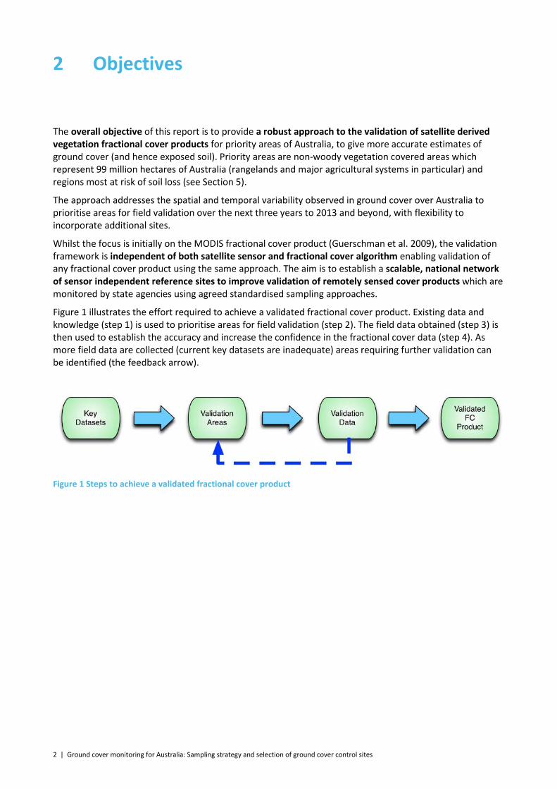
Figure 1 illustrates the effort required to achieve a validated fractional cover product. Existing data and knowledge (step 1) is used to prioritise areas for field validation (step 2). The field data obtained (step 3) is then used to establish the accuracy and increase the confidence in the fractional cover data (step 4). As more field data are collected (current key datasets are inadequate) areas requiring further validation can be identified (the feedback arrow).
Figure 1 Steps to achieve a validated fractional cover product
Ground cover monitoring for Australia: Sampling strategy and selection of ground cover control sites | 3
3 Outcomes
The desired outcomes of the validation sampling strategy are to:
• establish the accuracy of fractional cover products across the priority environments. The desired accuracy, set by the requirements of the CEMSYS and SedNet erosion models, is +/- 15% of the bare ground component (J. Leys and P. Hairsine, pers. comms.).
• reduce uncertainty, and hence increase accuracy of the products, achieved by:
– increasing confidence in the products as more validation information is acquired (by reducing the confidence interval of the prediction)
– modifications to the existing fractional cover algorithm.

4 | Ground cover monitoring for Australia: Sampling strategy and selection of ground cover control sites
4 The Expert Workshop
An Expert Workshop on Sampling Strategy and Selection of Ground Cover Control Sites was held at CSIRO Land and Water, Black Mountain, Canberra on the 17–18 August 2010 (Appendices 3 and 4). The workshop brought together 13 experts from federal and state agencies to discuss the development of a statistically robust sampling strategy for ground cover validation.
At the outset of the meeting, it was intended that the sampling strategy would:
• address the spatial and temporal variability observed in ground cover over Australia (in particular its major agricultural systems and rangelands)
• consider the current focus on the rangelands (Section 5) • on the basis of knowledge at the time, consider the perceived limitations of the current version of the
MODIS fractional cover product (Appendix B) and prioritise areas to target for field validation • identify the principles by which the number and likely locations of validation sites can be established on
the basis of the prioritised areas (Section 6) • consider existing suitable validation sites in the rangelands and the proposed Terrestrial Ecosystem
Research Network (TERN) validation sites.
Additionally, the meeting also discussed:
• the need for flexibility—to incorporate additional sites should the budget for validation effort increase, or target changed priority areas or conduct repeat validation visits on the basis of new information
• the limitations of the models that will use the fractional cover data (e.g. CEMSYS, SedNet) and the reliability of the ground cover data they require
• adopting the field sampling method for site description and measurement based on the Queensland DERM Statewide Land Cover And Trees Study (SLATS) modified discrete point sampling method along 100 metre transects, using the star-shaped transect approach (Scarth et al. 2006) for pastoral environments and the cross-transect method (Schmidt et al. 2010) for agricultural crops sown in lines
• the often conflicting criteria for validation site selection, the need for statistical rigour and the practicalities of implementing the sampling strategy.
4.1 Summary of workshop discussion
The workshop began by stating the importance for ground cover and soil condition information to assess impacts of the Caring for our Country program and of the importance of erosion modelling in that process. The MODIS fractional cover product is seen as the first step in monitoring ground cover at higher resolution allowing for an initial assessment of variation in ground cover through time and space. The need for a ground validation effort to establish confidence in the data was recognized given the limited validation of the product to date. The aims of the sampling strategy were outlined.
The conceptual basis for the fractional cover algorithm (Guerschman et al. 2009, Appendix A) was outlined and its value as a tool for assessing changes over time was discussed. Using local expert knowledge and the output flag analysis (Appendix B) a qualitative evaluation of product accuracy for selective areas was discussed. Although the accuracy of the current fractional cover product was not known, those who had used it felt it was accurate in relative terms, such as showing trends in ground cover fractions over time.
The spectral and spatial limitations of the MODIS sensor data were recognized. It was acknowledged that the fractional cover algorithm may overlook useful spectral information available in Landsat and MODIS sensor data and utilized in other ground cover unmixing approaches. The need to establish the current algorithm’s representativeness across the continent was recognized given that data from the Northern

Ground cover monitoring for Australia: Sampling strategy and selection of ground cover control sites | 5
Territory were used to establish current end-member locations. Similarly, the suitability of the BS/NPV/PV triangle being fixed with respect to time and space also required evaluation.
Alternative approaches to developing a sampling strategy were discussed including index-based site selection approaches. This approach proposed to use remote sensing indices which form the basis of the fractional cover algorithm (Appendix A) to identify areas to be focused on geographically; however, it was felt this approach would potentially overlook spectral variation not represented in the fractional cover triangle itself. A second approach proposed the use of stratified approaches enabled through multi-criteria decision support analysis of existing geographical information (e.g. land cover, soils, and access data). The coarse resolution of this approach (5 km) limited its use in identifying specific sites for validation but it was agreed this method could be a useful approach to communicate the process (Lesslie et al. 2008).
The required accuracy and reliability of the fractional cover data was also discussed. As the ground cover data will be used as an input into wind and water erosion modelling, the model requirements drive the need for reliability. For CEMSYS data precision was established as +/- 15% of the bare ground component (J. Leys, pers. comm.). SedNet needs the cover fractions (in particular differentiation between bare soil and non-photosynthetic vegetation) to predict sheet and rill erosion. Previously, 2001 National Land and Water Resources Audit cover satellite-based time series data was used giving an over-estimation of erosion in northern and central Australia (Hairsine et al. 2009). Data precision for SedNet for fractional cover was similarly established as +/- 15% (P. Hairsine, pers. comm.). Thus, for both models if an estimated fractional cover value for a pixel falls within this precision range it is considered accurate.
The experts agreed that there was no developed approach for allocating samples for broad-scale spectral unmixing which could be adopted for the fractional cover validation effort. Although the two approaches proposed above were useful, it was felt there was insufficient information on the variation in spectra of the different key landscape components to calculate explicit sample sizes to achieve a particular product precision. In the absence of this information the workshop used the practical experience of the participants to consider the number of validation sites necessary to cover areas where it is known the algorithm works well (‘validation’, to establish levels of confidence in the data) and on specific land classes shown to be problematic in the qualitative validation (Appendix B, ‘calibration’, to allow for algorithm improvement). Primarily, this included rangeland areas dominated by grassland and shrublands, with gibber, red, black, and bright soils. As this represents most of the rangelands, it was agreed that validation over wide spatial scales was the initial priority and, as validation information increased, to focus on spatio-temporal sampling. An initial validation analysis based on existing field data, available for Queensland and parts of NSW, was also recommended.
The expert group acknowledged the need to focus effort on priority areas of rangelands (as key sources of wind erosion), with additional effort on croplands (which would require higher temporal resolution ~4 times a year to capture the nature of their variability in cover fractions) (Stewart et al. 2011). Moreover, the need for temporal sampling, at some stage, was recognized, to capture growth response cover changes (e.g. in agricultural areas and following recent rains) to determine temporal reliability of the data. However, in the absence of sufficient spatial validation data, the initial prioritization of sampling sites would be based on spatial coverage, with site revisits planned for later sampling seasons.
The practicalities of implementing a sampling strategy were also discussed. The need for sampling sites to be suitable for the resolution of the MODIS product (500 metres) was recognized. Discussion also focused on the robustness of the SLATS sampling method and the contributions to error from its extent (100 x 100 metres compared to MODIS pixel size), radial pattern and from operator error. The value in using Landsat data to assist the site selection process (through assessment of homogeneity) was recognized as was allowing field teams flexibility to determine the ultimate location of a sampling site using local knowledge.
The workshop recommended a stratification guided by principles. These principles ensure sampling effort is representatively spread across areas of interest using agreed criteria for site selection (Section 6).
The workshop recommended that the sampling strategy be adaptive, with reviews undertaken annually to modify effort as validation information increased. An ongoing analysis would allow the assessment of soil, vegetation and spectral classes that may have been overlooked as well as expansion of the sampling effort should more resources become available.
6 | Ground cover monitoring for Australia: Sampling strategy and selection of ground cover control sites
4.2 Workshop conclusions and recommendations
• The absence of existing validation data (with the exception of Queensland and a limited set of sites in New South Wales), make it a non-trivial task to determine statistically the number of validation sites required to establish confidence in the data.
• Reliability of the fractional product is driven by the models that will ultimately use the data (e.g. CEMSYS wind erosion and SedNet sediment erosion models). An aspirational aim of +/- 15% of the bare ground component was agreed focussing on the relative accuracy of the signal over time.
• A preliminary analysis of existing Queensland and New South Wales validation data, and any new validation measurements should be undertaken as part of the first validation exercise. This will give an informed idea of the actual number of sites required statistically. As the validation data set increases, any reductions in variance can be assessed.
• Sampling sites should be representative at the MODIS resolution scale (500 metres). • Initial principles for validation site selection include: all non-woody vegetated areas used for agriculture
(grazing and broadacre cropping); a focus on the rangelands with limited emphasis on croplands; full range of ground covers (0 – 100% for each cover fraction) sampled and soil colours targeted known to affect algorithm performance. These principles are elaborated in Section 6.
• Validation sites should be spread spatially using a stratification method (Section 6) but prioritised on what states can reasonably access, including the use of existing suitable sites.
• An iterative sampling strategy should be implemented, initially with wide spatial coverage and limited temporal coverage. Sampling effort should be annually reviewed and adapted to meet identified information needs (e.g. sites poorly represented in field data already obtained) and the inclusion of new sampling sites if resources become available. Site revisits to assess temporal variability should be planned for later sampling.
Figure 2 illustrates the validation approach with the activities required to achieve a sampling strategy and process for achieving the desired accuracy of the fractional cover product. The process for making future decisions around the sampling strategy, in the form of annual review, algorithm modification and refinement of the sampling sites is also shown. The activities required are:
Stratification – using datasets and principles addressing variability to prioritise areas for targeted field validation. In so doing, the likely number of samples required is identified. This activity represents the main thrust of this report (Section 6).
Field validation – the acquisition of field data to establish accuracy of the fractional cover product. This is guided by 1) a sampling protocol, used to assist site selection (Appendix E), and 2) a sampling handbook, so that the field cover data is obtained in a standardised manner (Muir et al. 2011).
Validation analysis and annual review – an assessment of the validation progress to determine 1) the overall uncertainty in the fractional cover product, 2) the adequacy of the field measurement campaign to achieve this goal and 3) to inform the number of sampling sites ultimately required. Section 7 gives the framework for this activity.
Algorithm modification – improvements in the fractional cover algorithm to meet desired accuracies specified for the product. Briefly covered in Section 7.
Refinement of areas of interest – refinement and modification of the sampling effort to address new priorities for field validation identified in the validation analysis. Elements of these priorities are outlined in Section 7.

Ground cover monitoring for Australia: Sampling strategy and selection of ground cover control sites | 7
Figure 2 Recommended sampling and validation strategy for the fractional cover product
8 | Ground cover monitoring for Australia: Sampling strategy and selection of ground cover control sites
5 Areas of interest
5.1 Rangelands
“The rangelands encompass tropical woodlands and savannas in the far north; vast treeless grassy plains (downs country) across the mid-north; hummock grasslands (spinifex), mulga woodlands and shrublands through the mid-latitudes; and saltbush and bluebush shrublands that fringe the agricultural areas and Great Australian Bight in the south. Across this gradient, seasonal rainfall changes from summer-dominant (monsoonal) in the north to winter-dominant in the south. Soils are characteristically infertile. Great climate variability and the dominating influence of short growing seasons distinctly characterise rangeland environments.” (Bastin et al. 2008)
The rangelands are defined here as those areas where the rainfall is too low or unreliable and the soils too poor to support regular cropping (Bastin et al. 2008). They cover approximately 81% of Australia comprising predominantly the arid and semiarid interior and the monsoonal north and include diverse savannas, woodlands, shrublands, grasslands and wetlands. The IBRA regionalization (Thackway and Cresswell 1995) identifies 52 bioregions1
Agricultural production—principally extensive grazing of many grassland types—in the rangelands is widespread; 3.2 million km2 of the rangelands (more than 43% of Australia) are grazed (McKeon et al. 2004). The rangelands thus have significant economic, social and cultural values and given their extensive size play a significant role in carbon storage.
or parts of bioregions in the rangelands. The rangelands thus contain a rich diversity of species and habitats with many habitats remaining relatively unmodified but extremely vulnerable to change.
The defining characteristic of the rangelands is variability in both space and time. Rainfall varies greatly from year to year, season to season with change principally driven by episodic cycles of drought and wet periods. Water is a key force defining land use and management. Other drivers of change include extensive grazing of natural vegetation by domestic livestock and feral pests (occurring across most of the rangelands), fire, land clearance of wooded regions leading to habitat loss and fragmentation, and exotic weed invasions. All these influences affect how well rangeland landscapes retain resources. Many of these pressures can accelerate soil erosion and alter vegetation composition and structure and hence affect fractional cover. Functional landscapes are identified as having high cover of more persistent patches of perennial vegetation, which are spatially arranged to efficiently capture rainfall and runoff and resist wind erosion.
The high variability in the rangelands means that assessing change is particularly difficult: change can be slow and hard to detect, or it can occur rapidly (Bastin et al. 2008). Mapping and monitoring is a considerable challenge because of the large area, spatial complexity and temporal variability of the arid zone vegetation. Stocking densities of grazers varies (linked to the underlying inherent primary productivity of pastoral bioregions) such that grazing impacts are highly variable. The scale and variability in Australia's rangelands presents a significant challenge, not only in obtaining adequate baseline data, but in assessing trends, and identifying the causes of change. This variability translates into wide variability in observed fractional cover.
1 A bioregion is a large, geographically distinct area of land and/or water that has assemblages of ecosystems forming recognizable patterns within the landscape

Ground cover monitoring for Australia: Sampling strategy and selection of ground cover control sites | 9
5.2 Broadacre cropping
Broadacre cropping covers ~8% of the country (> 200,000 km2) in a belt that runs down the east coast of Australia, around the south coast and halfway up the west coast. One to two crop cultivations per year are typical—with most cropping land left fallow for 3–9 months. These periods are likely to be dominated by high non-photosynthetic vegetation (stubble) cover or bare soil (~68% of cropped areas are left intact, 18% have residue removed; Barson et al. 2012). Zero till is a common practice which attempts to maintain soil cover. As for rangelands the distribution of cropping is driven by climatic factors, particularly rainfall amounts, timing and reliability, while at the local scale soil and landscape features are important. The most intensive land use is generally in the wetter temperate parts of Australia. The variations in climate and resulting variations in cropping management mean highly variable fractional cover proportions in both space and time.
For both these agricultural systems, the response of vegetation to climate variability (i.e. transitions into drought followed by recovery after sustained rainfall) is the main effect that the fractional cover product will ultimately monitor (although variable stocking rates may contribute to variation in this response).
The agricultural landscapes of Australia support a diversity of soils with most ancient and low in both organic content and fertility. Combined with climatic interactions and human impacts, sustainable agricultural systems are difficult to develop (ANRA 2009). Soils contribute to the diversity of vegetation response and highly varying rates of erodibility. Variations in soil colour are also wide and are highly likely to influence the fractional cover algorithm retrieval.
10 | Ground cover monitoring for Australia: Sampling strategy and selection of ground cover control sites
6 Stratification
This section outlines the stratification activity to identify specific sites for field validation. Principles are proposed to define priority validation areas, the key datasets for the stratification are given and the initial, likely number of samples required is established.
6.1 Principles
A set of principles were drafted at the Expert Workshop for the sampling strategy. These principles aim to achieve the desired outcome of +/- 15% accuracy of the bare ground component while addressing variability and the need to stratify the location of sampling sites.
The overarching principles, in order of their priority and with brief justifications, are:
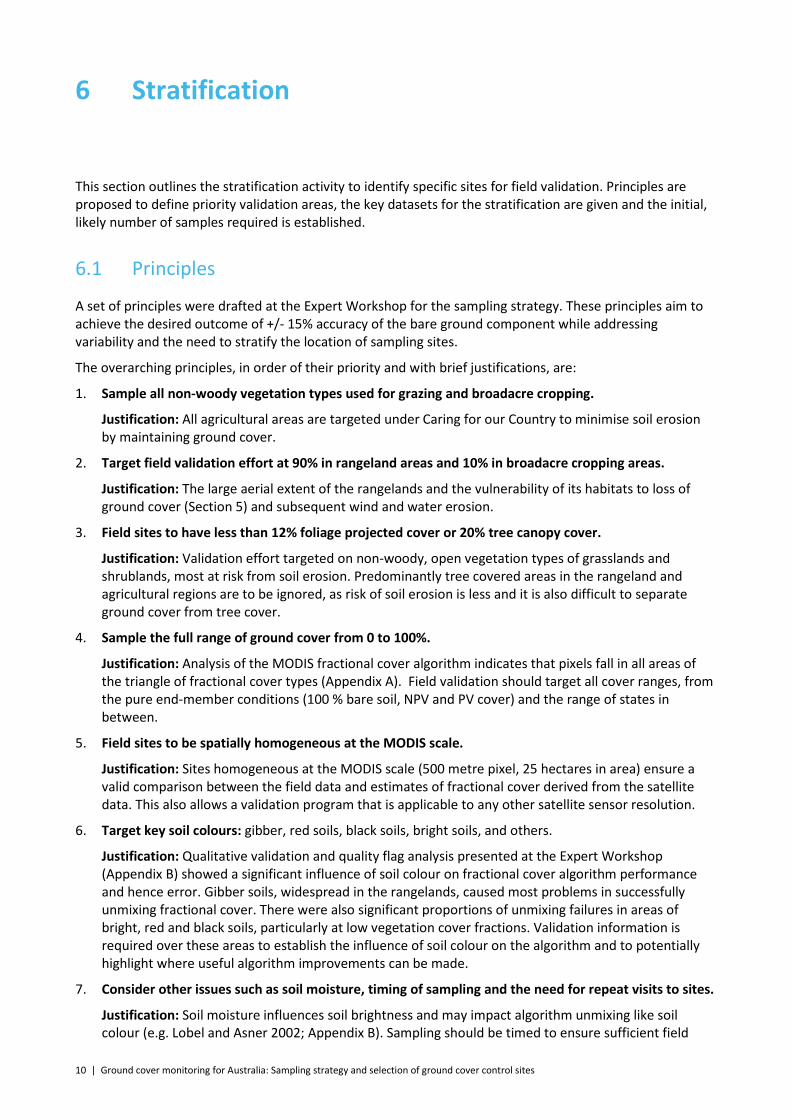
1. Sample all non-woody vegetation types used for grazing and broadacre cropping.
Justification: All agricultural areas are targeted under Caring for our Country to minimise soil erosion by maintaining ground cover.
2. Target field validation effort at 90% in rangeland areas and 10% in broadacre cropping areas.
Justification: The large aerial extent of the rangelands and the vulnerability of its habitats to loss of ground cover (Section 5) and subsequent wind and water erosion.
3. Field sites to have less than 12% foliage projected cover or 20% tree canopy cover.
Justification: Validation effort targeted on non-woody, open vegetation types of grasslands and shrublands, most at risk from soil erosion. Predominantly tree covered areas in the rangeland and agricultural regions are to be ignored, as risk of soil erosion is less and it is also difficult to separate ground cover from tree cover.
4. Sample the full range of ground cover from 0 to 100%.
Justification: Analysis of the MODIS fractional cover algorithm indicates that pixels fall in all areas of the triangle of fractional cover types (Appendix A). Field validation should target all cover ranges, from the pure end-member conditions (100 % bare soil, NPV and PV cover) and the range of states in between.
5. Field sites to be spatially homogeneous at the MODIS scale.
Justification: Sites homogeneous at the MODIS scale (500 metre pixel, 25 hectares in area) ensure a valid comparison between the field data and estimates of fractional cover derived from the satellite data. This also allows a validation program that is applicable to any other satellite sensor resolution.
6. Target key soil colours: gibber, red soils, black soils, bright soils, and others.
Justification: Qualitative validation and quality flag analysis presented at the Expert Workshop (Appendix B) showed a significant influence of soil colour on fractional cover algorithm performance and hence error. Gibber soils, widespread in the rangelands, caused most problems in successfully unmixing fractional cover. There were also significant proportions of unmixing failures in areas of bright, red and black soils, particularly at low vegetation cover fractions. Validation information is required over these areas to establish the influence of soil colour on the algorithm and to potentially highlight where useful algorithm improvements can be made.
7. Consider other issues such as soil moisture, timing of sampling and the need for repeat visits to sites.
Justification: Soil moisture influences soil brightness and may impact algorithm unmixing like soil colour (e.g. Lobel and Asner 2002; Appendix B). Sampling should be timed to ensure sufficient field

Ground cover monitoring for Australia: Sampling strategy and selection of ground cover control sites | 11
visits, and hence data, across annual cycles of growth (PV dominated) and senescence (NPV dominated) in rangeland areas. Repeated sampling of sites already visited will be an additional component of the annual reviews in subsequent years, particularly in cropping areas where it will be necessary to capture variations in ground cover through seasonal growth cycles. Repeated sampling helps to establish the temporal reliability of the product.
8. Through review, ensure an adequate number of sites in each priority environment.
Justification: Priority areas need to be adequately sampled and visited for field ground cover data (across potentially 90 classes of ground cover—high, medium, low for the three components, covering the 5 soil colour classes, and 2 soil moisture levels—dry and wet). The steps to achieve this are outlined in Section 7.
These principles are independent of both a specific fractional cover algorithm and satellite sensor. They address variability in priority areas to provide a framework for the sampling stratification. The approach ensures that the field data can be used to both calibrate and validate any ground cover product and to assist improvement in product accuracy. They are also intended to ensure that field validation is representative across Australia.
6.2 Datasets required
Spatial datasets used in the sampling site stratification process are:
1. Rangelands boundary (Figure 3a) – based on the Australian Collaborative Rangeland Information System (ACRIS) boundary (Bastin et al. 2008). Used to ensure that 90% effort is targeted in this zone.
2. Agricultural / non agricultural area binary classification (Figure 3b) – generated from a reclassification of Catchment scale land use of Australia - update March 20102
3. Forest cover (Figure 3c) – derived from the Forests of Australia 2008
. Used to eliminate non-agricultural areas. The data derived are indicative only for parts of the rangelands and could be improved by merging with the national land use product.
3
4. Foliage projective cover (Figure 3d) – defined as the percentage of ground area occupied by the vertical projection of foliage and developed principally for determining trends in woody vegetation (Montreal Process Implementation Group for Australia 2008)
dataset, and used to eliminate areas of dominant tree cover from the analysis.
4
5. Soil colour (Figure 3e) – dataset derived from the Digital Atlas of Australian Soils
. Used to eliminate areas of woodland and tree cover from the analysis not identified in dataset 3, such that the focus is on grassland and shrubland cover types.
5 based on 1:2.5 million scale maps of the Northcote soil classification (Northcote et al. 1960–1968, Northcote 1979) and the Interim Biogeographic Regionalisation for Australia (IBRA) land surface of Australia (Thackway and Cresswell 1995). To formulate this dataset, advice on soil colour, by IBRA6
6. Land cover (Figure 3f) – use to identify areas used for broadacre cropping based on the National Dynamic Land Cover Dataset (Lymburner et al. 2011)
and sub IBRA regions was provided by jurisdictions and an expert panel. Used to broadly identify the five priority soil types identified for this study (gibber, bright soils, red soils, black soils and other).
7
2
http://adl.brs.gov.au/anrdl/metadata_files/pa_luausr9abll07611a00.xml
.
3 http://adl.brs.gov.au/anrdl/metadata_files/pa_foraug9abll0062008_11a.xml 4
http://adl.brs.gov.au/anrdl/metadata_files/pa_foraug9abll0062008_11a.xml 5
http://adl.brs.gov.au/anrdl/metadata_files/pa_daaslr9abd_00111a01.xml 6
http://www.environment.gov.au/metadataexplorer/full_metadata.jsp?docId=%7BAC901094-DA0D-4BF2-B957-3202AA189258%7D&loggedIn=false 7
http://www.ga.gov.au/earth-observation/landcover.html

12 | Ground cover monitoring for Australia: Sampling strategy and selection of ground cover control sites
Figure 3 Datasets used in the sampling stratification Note: Plantations in forest cover (map d) and bare and mining in land cover (map f) are present in the datasets but not visible at the scale shown
a b
c d
e f
Ground cover monitoring for Australia: Sampling strategy and selection of ground cover control sites | 13
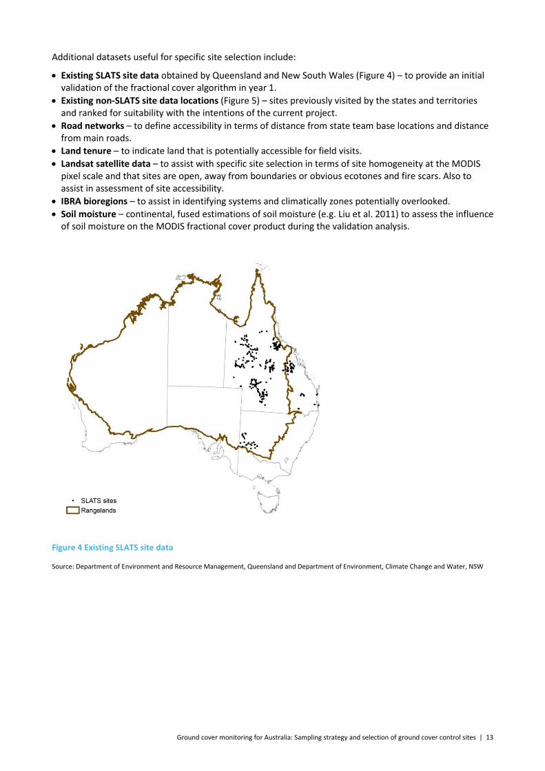
Additional datasets useful for specific site selection include:
• Existing SLATS site data obtained by Queensland and New South Wales (Figure 4) – to provide an initial validation of the fractional cover algorithm in year 1.
• Existing non-SLATS site data locations (Figure 5) – sites previously visited by the states and territories and ranked for suitability with the intentions of the current project.
• Road networks – to define accessibility in terms of distance from state team base locations and distance from main roads.
• Land tenure – to indicate land that is potentially accessible for field visits. • Landsat satellite data – to assist with specific site selection in terms of site homogeneity at the MODIS
pixel scale and that sites are open, away from boundaries or obvious ecotones and fire scars. Also to assist in assessment of site accessibility.
• IBRA bioregions – to assist in identifying systems and climatically zones potentially overlooked. • Soil moisture – continental, fused estimations of soil moisture (e.g. Liu et al. 2011) to assess the influence
of soil moisture on the MODIS fractional cover product during the validation analysis.
Figure 4 Existing SLATS site data
Source: Department of Environment and Resource Management, Queensland and Department of Environment, Climate Change and Water, NSW
14 | Ground cover monitoring for Australia: Sampling strategy and selection of ground cover control sites
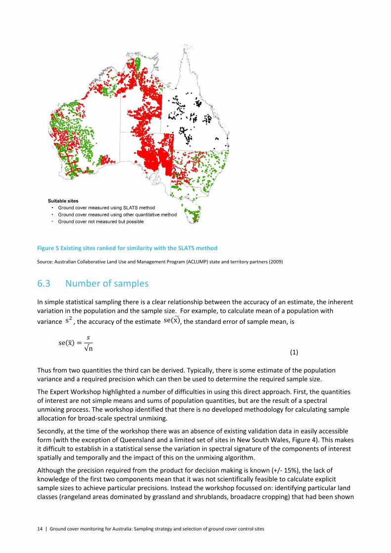
Figure 5 Existing sites ranked for similarity with the SLATS method
Source: Australian Collaborative Land Use and Management Program (ACLUMP) state and territory partners (2009)
6.3 Number of samples
In simple statistical sampling there is a clear relationship between the accuracy of an estimate, the inherent variation in the population and the sample size. For example, to calculate mean of a population with variance , the accuracy of the estimate , the standard error of sample mean, is
(1)
Thus from two quantities the third can be derived. Typically, there is some estimate of the population variance and a required precision which can then be used to determine the required sample size.
The Expert Workshop highlighted a number of difficulties in using this direct approach. First, the quantities of interest are not simple means and sums of population quantities, but are the result of a spectral unmixing process. The workshop identified that there is no developed methodology for calculating sample allocation for broad-scale spectral unmixing.
Secondly, at the time of the workshop there was an absence of existing validation data in easily accessible form (with the exception of Queensland and a limited set of sites in New South Wales, Figure 4). This makes it difficult to establish in a statistical sense the variation in spectral signature of the components of interest spatially and temporally and the impact of this on the unmixing algorithm.
Although the precision required from the product for decision making is known (+/- 15%), the lack of knowledge of the first two components mean that it was not scientifically feasible to calculate explicit sample sizes to achieve particular precisions. Instead the workshop focussed on: identifying particular land classes (rangeland areas dominated by grassland and shrublands, broadacre cropping) that had been shown
s2 se(x)�
se(x�) =𝑠𝑠√n

Ground cover monitoring for Australia: Sampling strategy and selection of ground cover control sites | 15
to be problematic in earlier qualitative validation as areas that would provide maximum information and; sampling protocols at local areas to deal with spatial and temporal scaling issues (Sections 6.1 and 6.2).
A credible sampling scheme is presented. The approach taken is consistent with the workshop discussions. The workshop endorsed that the process of developing any product of this size will be iterative; as data is collected and resources committed to its analysis greater clarity will be achieved about the information needs for a national product (outlined in Section 8).
6.3.1 INDICATIVE SAMPLE NUMBER
The development of an indicative sampling scheme for fractional cover validation is best begun by considering what can be learned from other existing national remote sensing products. The primary example in Australia is the land cover product used in the National Carbon Accounting System (NCAS, Furby 2002). This product uses sophisticated classifiers rather than spectral unmixing so comparisons have to be made cautiously. However, it is still the only operational continental remote sensing monitoring product.
At its inception the NCAS project collected multiple samples from 800 aerial photos across all 85 IBRA bioregions in Australia (Lowell et al. 2003). This initial sample set did not produce sufficiently accurate estimates of land cover over all of Australia so an additional sample of 1000 10 km by 10 km IKONOS satellite images were obtained and multiple calibration samples derived from these. This produced a dataset of around 3000 samples to be used for validation (P. Caccetta, pers. comm.). Samples were distributed stratified firstly by soil and vegetation type and then by change/state class and were located by visual inspection.
Whether 3000 is an appropriate number of samples is debatable. Given this level of sampling there are still issues with the accuracy of the NCAS data for a number of applications. Against this, there are potential efficiencies that can be achieved when using spectral unmixing approaches such as that used in the fractional cover algorithm, as opposed to the hard classification approach adopted in NCAS. Firstly, unsupervised methods can be used to extract additional signal information from the entire image. Secondly, certain spectral signals may lack variation over larger regions; indicating the spectral consistency of objects across the space—if an object has more consistent variation across space then it may require a lower intensity of sampling effort. Thirdly, error in spectral signal may have less of an effect when detecting changes rather than current state (in other words, it may be easier to detect the relative changes in an object and with less error than in performing object classification first and using that as the basis for the change detection). On the basis of this, and following discussions with Mark Berman, an international expert on spectral unmixing with experience in its application to remote sensing, it was considered that 1000-1500 sites would be a credible sample, provided that they contained a reasonable number of relatively pure pixels (to reduce error), established by targeting large, homogeneous areas. Given this, the following discussion assumes a sample of 1500 sites. It is unlikely that a broadly credible national product could be constructed with fewer samples, and the requirement may be higher.
6.3.2 INDICATIVE SAMPLING SCHEME
Given that the Expert Workshop identified reasonably quickly that there was no way of calculating ‘required’ sample sizes, and that initial funding provided for a relatively low number of sites (~500), discussion concentrated on prioritising locations for sampling and the protocols for the different jurisdictions. To envisage a national sampling regime requires additional considerations. These are:
• On a purely statistical basis it is recommended that the sample be distributed systematically across the in-scope region. This has a number of advantages. Firstly, it gives maximum spatial representation, and in the absence of information about the spatial patterns of variation this is prudent. A systematic sample, however, has the weakness of not providing spatial information locally to a sample point, but this should not be an issue in this case. A systematic sample should also be approximately self-weighting, such that each pixel is equally ‘representative’. A systematic spatial sample will allocate samples approximately proportional to the area of any spatial strata.
16 | Ground cover monitoring for Australia: Sampling strategy and selection of ground cover control sites
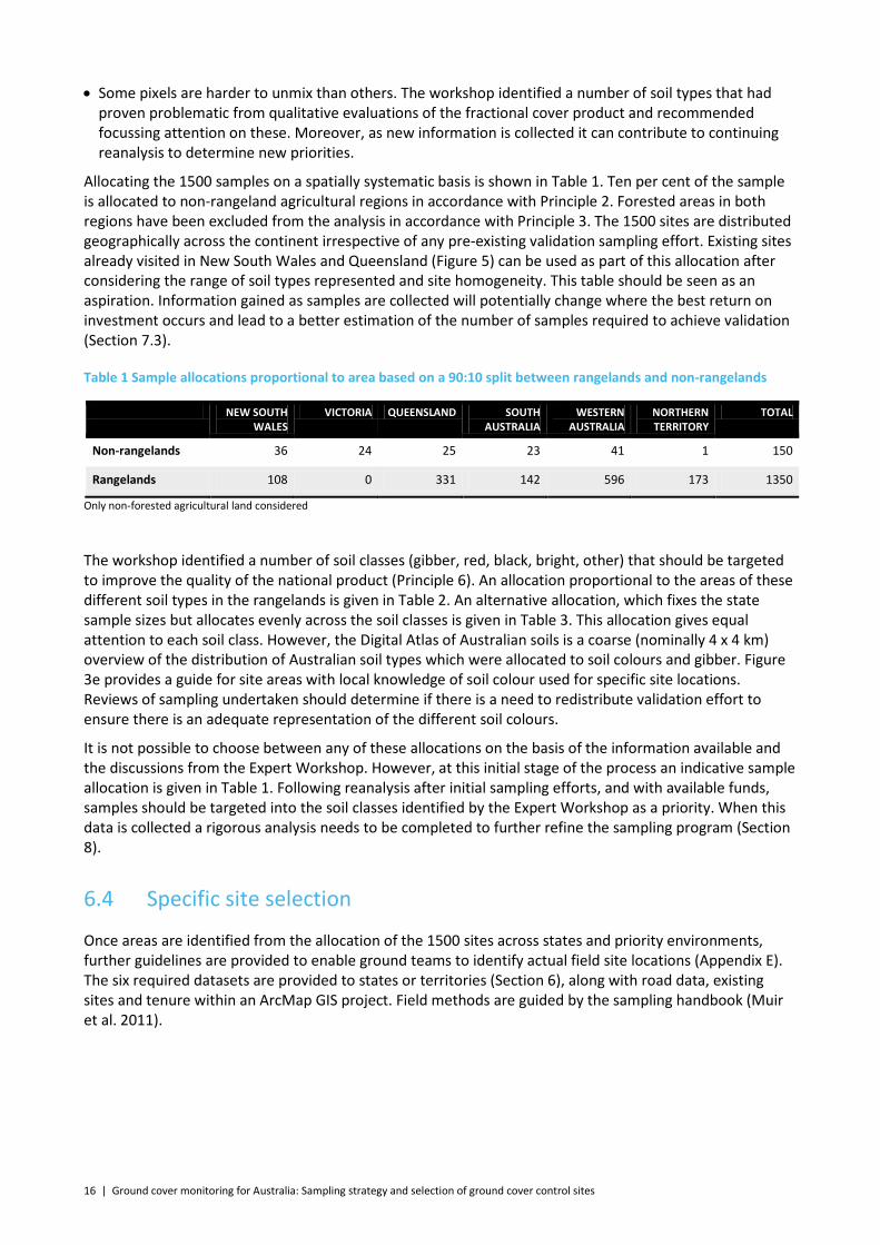
• Some pixels are harder to unmix than others. The workshop identified a number of soil types that had proven problematic from qualitative evaluations of the fractional cover product and recommended focussing attention on these. Moreover, as new information is collected it can contribute to continuing reanalysis to determine new priorities.
Allocating the 1500 samples on a spatially systematic basis is shown in Table 1. Ten per cent of the sample is allocated to non-rangeland agricultural regions in accordance with Principle 2. Forested areas in both regions have been excluded from the analysis in accordance with Principle 3. The 1500 sites are distributed geographically across the continent irrespective of any pre-existing validation sampling effort. Existing sites already visited in New South Wales and Queensland (Figure 5) can be used as part of this allocation after considering the range of soil types represented and site homogeneity. This table should be seen as an aspiration. Information gained as samples are collected will potentially change where the best return on investment occurs and lead to a better estimation of the number of samples required to achieve validation (Section 7.3).
Table 1 Sample allocations proportional to area based on a 90:10 split between rangelands and non-rangelands
NEW SOUTH WALES
VICTORIA QUEENSLAND SOUTH AUSTRALIA
WESTERN AUSTRALIA
NORTHERN TERRITORY
TOTAL
Non-rangelands 36 24 25 23 41 1 150
Rangelands 108 0 331 142 596 173 1350
Only non-forested agricultural land considered
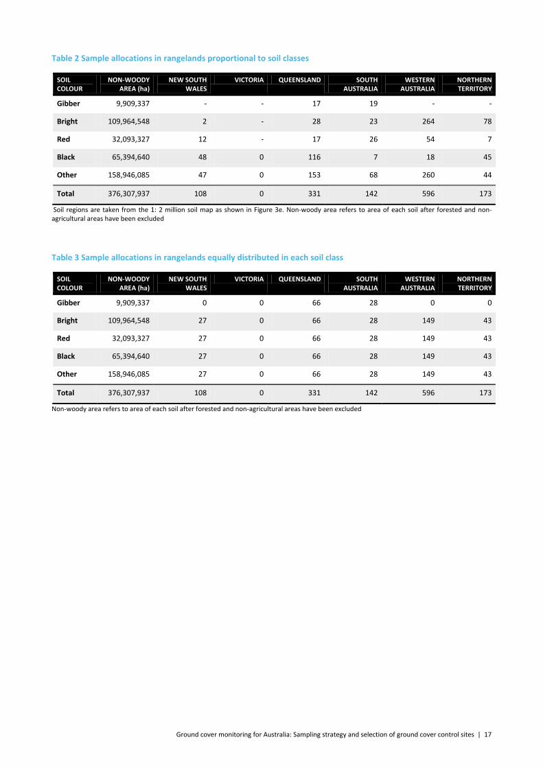
The workshop identified a number of soil classes (gibber, red, black, bright, other) that should be targeted to improve the quality of the national product (Principle 6). An allocation proportional to the areas of these different soil types in the rangelands is given in Table 2. An alternative allocation, which fixes the state sample sizes but allocates evenly across the soil classes is given in Table 3. This allocation gives equal attention to each soil class. However, the Digital Atlas of Australian soils is a coarse (nominally 4 x 4 km) overview of the distribution of Australian soil types which were allocated to soil colours and gibber. Figure 3e provides a guide for site areas with local knowledge of soil colour used for specific site locations. Reviews of sampling undertaken should determine if there is a need to redistribute validation effort to ensure there is an adequate representation of the different soil colours.
It is not possible to choose between any of these allocations on the basis of the information available and the discussions from the Expert Workshop. However, at this initial stage of the process an indicative sample allocation is given in Table 1. Following reanalysis after initial sampling efforts, and with available funds, samples should be targeted into the soil classes identified by the Expert Workshop as a priority. When this data is collected a rigorous analysis needs to be completed to further refine the sampling program (Section 8).
6.4 Specific site selection
Once areas are identified from the allocation of the 1500 sites across states and priority environments, further guidelines are provided to enable ground teams to identify actual field site locations (Appendix E). The six required datasets are provided to states or territories (Section 6), along with road data, existing sites and tenure within an ArcMap GIS project. Field methods are guided by the sampling handbook (Muir et al. 2011).
Ground cover monitoring for Australia: Sampling strategy and selection of ground cover control sites | 17
Table 2 Sample allocations in rangelands proportional to soil classes
SOIL COLOUR
NON-WOODY AREA (ha)
NEW SOUTH WALES
VICTORIA QUEENSLAND SOUTH AUSTRALIA
WESTERN AUSTRALIA
NORTHERN TERRITORY
Gibber 9,909,337 - - 17 19 - -
Bright 109,964,548 2 - 28 23 264 78
Red 32,093,327 12 - 17 26 54 7
Black 65,394,640 48 0 116 7 18 45
Other 158,946,085 47 0 153 68 260 44
Total 376,307,937 108 0 331 142 596 173
Soil regions are taken from the 1: 2 million soil map as shown in Figure 3e. Non-woody area refers to area of each soil after forested and non-agricultural areas have been excluded
Table 3 Sample allocations in rangelands equally distributed in each soil class
SOIL COLOUR
NON-WOODY AREA (ha)
NEW SOUTH WALES
VICTORIA QUEENSLAND SOUTH AUSTRALIA
WESTERN AUSTRALIA
NORTHERN TERRITORY
Gibber 9,909,337 0 0 66 28 0 0
Bright 109,964,548 27 0 66 28 149 43
Red 32,093,327 27 0 66 28 149 43
Black 65,394,640 27 0 66 28 149 43
Other 158,946,085 27 0 66 28 149 43
Total 376,307,937 108 0 331 142 596 173
Non-woody area refers to area of each soil after forested and non-agricultural areas have been excluded
18 | Ground cover monitoring for Australia: Sampling strategy and selection of ground cover control sites
7 Validation analysis and annual review
At the beginning of each sampling year (2011, 2012 and 2013), adaptive reviews of the data collected and progress in validation are recommended. These reviews will determine the adequacy of the validation measurements undertaken in targeted areas of cover ranges and soil colours. To support this ongoing analysis will require additional investment.
The validation analysis will:
• assess the assumption that the 1500 sample size will provide enough information to give an informative validation of the fractional cover product and desired levels of confidence
• determine if sampling sites visited are sufficiently homogeneous at the MODIS scale and of reliable quality
• ascertain if a sufficient range in spectral coverage of data has been acquired. Redirect sampling effort if needed to meet this requirement for spectral coverage
• assess the impact of current ground cover sampling effort on the overall uncertainty of the product to determine i) new priority areas for targeted sampling ii) improvements in the fractional cover algorithm itself
• review timing of sampling to identify if validation effort has been adequately concentrated at key times of year (for example relative proportions of green (PV) versus dry (NPV) vegetation components)
• redirect sampling effort if needed to meet requirement for temporal coverage • identify additional areas where the algorithm needs improvement • consider the utility of the current product and raw data as new information from new sensors becomes
available.
As the multi-criteria approach to stratification is not an exact optimization, issues of the spatial representativeness of the validation can also be assessed at this stage. These tasks are not trivial and would require significant resourcing.
Achieving validation is an iterative activity, refined over several years of effort.
7.1 Why collect more data?
Collecting additional data is useful for model calibration and validation. The following examples (Figure 6) use the analogy of a model estimate (y axis) derived from one or more independent variables (x axis) through a simple mathematical equation. Here, the estimated variable is ground cover and the independent variables are the reflectances derived from remote sensing data.
The examples demonstrate that the collection of field data serves the double purpose of:
• ensuring that all the potential (environmental) conditions where the model intends to be used are covered. In other words, the model is not extrapolated to conditions where it does not work
• new observations can be used as independent validation of the model.
Figure 6a illustrates the initial situation where a first set of field observations (n = 10) range from x = 1 to x = 10. A linear model fits the data well. Twenty additional observations are collected (Figure 6b). The range of x now spans from 1 to 20. The initial, linear, model still fits the data well, but makes poor predictions in overestimating those observations ranging from x = 11 to 20.
The same model structure, that is a linear fit, is re-calibrated using all the available observations (n=30, Figure 6c). Now the model performs worse than the initial one (as evidenced through the decreased r2) and also seems to over predict the estimated variable at low (x < 5) and high (x > 15) values and under predict when x is between 5 and 15.

Ground cover monitoring for Australia: Sampling strategy and selection of ground cover control sites | 19
Figure 6 Theoretical explanation of model improvement as validation effort expands a) initial situation (blue circles), b) addition of first validation samples (red circles) with initial linear model c) recalculated linear model to all validation data, d) recalculated non‐linear model to all validation data, e) addition of further validation data (yellow dots)
The data suggests that a linear model is not appropriate to represent the observed data. A logarithmic model does a better job (Figure 6d). Now the model fits the observations much better than the linear model. Finally, another 20 observations are collected spanning the same range of x (1 to 20) and the model is tested on those data (Figure 6e).
The validation of the MODIS fractional cover algorithm, with information lacking upon which to base a validation effort is effectively the situation of Figure 6a. There is a model and a set of very few validation
a
e
dc
b
20 | Ground cover monitoring for Australia: Sampling strategy and selection of ground cover control sites
points. More points are required to test if the same model applies as the validation is expanded spatially and into priority areas (such as different soil colours, vegetation types, etc).
The example demonstrates that as time progresses the accuracy of the model can be increased through reducing the confidence interval of the prediction as there is a greater number of validation sites. Although overall variance may not change, more samples means increased model confidence can be achieved.
7.2 Steps to validation
7.2.1 ASSESS SITE HETEROGENEITY
The first step in a validation analysis will be to assess how representative the fractional cover data obtained at specific field sites using the SLATS method (three 100 metre transects arranged in a star shape) are compared to the MODIS scale (500 metres, equivalent to 25 hectares). The recommended steps to determine this are:
• select the closest available cloud free Landsat image (30 metre resolution) to the date of the field visit • define the equivalent of the MODIS pixel (500 metres) around the field site • estimate the spectral variability around the field site that is evident in the Landsat data • categorically classify heterogeneity into 3 classes (low, medium and high heterogeneity).
Validation analysis should then proceed on the basis of sites differentiated by their relative heterogeneity (i.e. to determine if heterogeneity is positively associated with model error).
7.2.2 ASSESS VALIDATION DATA OBTAINED
Through basic descriptive statistics and geospatial analysis, assess the range of covers represented:
• In the three cover fractions (PV, NPV, and BS) in ranges from absent to full cover. Identify cover fractions significantly overlooked, potentially as a result of concentration of effort during one part of the year.
• In spatial distribution:
– coverage reflecting 90:10 effort split across rangelands and cropping areas, respectively (plotted against the rangelands boundary layer)
– across priority vegetation types (plotted against land cover layer). Identify key types potentially oversampled or overlooked
– across priority soil types and colours (plotted against soil layer). Identify key soil types/colours potentially oversampled or overlooked.
The analyses identify data gaps to inform priorities for validation effort in subsequent years. The spatial heterogeneity of areas should also be considered when determining the sampling effort. For example, desert regions may not need as much validation effort to adequately describe the heterogeneity represented.
7.2.3 COMPARE FIELD DATA WITH MODIS-DERIVED FRACTIONAL COVER
• Plot field observations (observed) against MODIS-derived fractional cover (predicted) for each of the three cover fractions (PV, NPV and BS).
• Assess the degree of agreement using Root Mean Square Error (RMSE), coefficient of determination (r2), and other statistics.
• Note any bias in the predictions and the dispersion of the data. • Validate the degree to which the algorithm under- or over-estimates cover fractions in different cover
ranges by plotting distributions of the predicted and observed covers. • Where useful, differentiate sites by region, soil colour and soil moisture, and site heterogeneity. Assess
any variations in the separate relationships and attempt to explain.
Ground cover monitoring for Australia: Sampling strategy and selection of ground cover control sites | 21
• From the flag outputs, differentiate the sites by unconstrained and constrained unmixing. Assess variations in the separate relationships and attempt to explain.
7.2.4 ASSESS PRIORITIES FOR REVISITING SITES
Whilst some analysis of temporal variation can be assessed using information from multiple-revisited sites in existing Queensland SLATS data, the need for repeated sampling of sites already visited should be a component of the annual review.
In cropping areas 3 to 4 repeat visits will be required to map changes over the crop growing cycle; revisiting other sites already measured allows the potential to capture growth response (e.g. to recent rains) and to get a sense of the temporal reliability of the fractional cover product by removing the spatial dimension. In the rangelands, temporal sampling allows for the validation of the precision of changes in the green and dry vegetation fractions through the seasonal cycle (i.e. with what precision can the fractional cover product detect change in the same place?).
7.2.5 ALGORITHM IMPROVEMENT
As outlined in Section 7.1, increasing the number of samples should increase model accuracy and highlight conditions under which the model is predicting poorly and requires modification.
Consideration should be given to the following when improving the model:
• poorly located end-members, poorly represented triangle shape – requirement for model recalibration • systematic biases in fractional cover estimation (over- and under-estimation) • the possibility that more variables (dimensions) are required (e.g. further spectral information) • the model is dynamic in time and space (end-members can change) • relaxing the assumption that the unmixing is linear. • data from alternative satellite sensors.
7.3 Determining the number of samples required
The validation effort is intended to increase the reliability of the fractional cover estimates. Monitoring progress to the goal of +/- 15% accuracy is fundamental to the validation activity.
When using satellite data to estimate fractional cover, errors will be introduced and will propagate through the processing chain. Sources of error are:
• processing related – caused by the design of the sensor and its calibration and characterisation, and to processing of the data through the processing chain—including suitability of radiometric calibration
• positional – related to the geometric accuracy of the image • scale related – due to the size of the pixel of the satellite data being used to estimate fractional cover • model related – a result of the fractional cover algorithm itself, estimation error in the model parameters
used and variation not explained by the model itself.
Similarly, there are also sources of error in the field estimation of fractional cover, caused by:
• estimation error in the fractions of cover by the operator • any bias in cover estimation introduced by the SLATS star-shaped transect technique • positional error in the location of the sample point and/or transects • scaling from ground-based measurements to the 500 metre MODIS pixel size – including the relative
homogeneity of the area measured to the pixel(s) that represents that area.
To fully understand the uncertainty associated with the estimation of fractional cover using MODIS satellite data would require the establishment of a full error budget. This would quantify the error from the possible sources highlighted above. For the purposes of this study, error is assumed to arise from the fractional

22 | Ground cover monitoring for Australia: Sampling strategy and selection of ground cover control sites
cover algorithm itself (considered the likely largest source of error in the estimation process), and from scaling differences between the ground-based measurement and the MODIS pixel.
7.3.1 DATA SIMULATION
Data simulation can be used to help estimate the number of samples needed. A number of paired ‘predicted versus measured’ observations are generated with random error introduced, each used to separately estimate regression parameters. The core steps in this approach are to:
• vary calibration sample size • for each sample size, add random error to each ‘predicted value’ estimated using the overall regression
between predicted and observed for all field observations • estimate the standard deviation of parameter estimates, developed from individual regression
parameters for many hundreds of independently simulated datasets for each calibration sample size • plot the relationship between sample size and parameter standard errors (Figure 7).
Figure 7 Simulated example of reduction in prediction error with increasing calibration sample size
7.3.2 UNDERSTANDING ERRORS DUE TO SCALING
In the validation process, as more samples become available from the field teams over time, the error (uncertainty) in estimation of fractional cover should decrease. In future validation analyses, higher spatial resolution data (e.g. from Landsat, 30 metre resolution) could be used to ‘bridge’ between the field sample and MODIS scale estimates of fractional cover. This approach is implemented by first relating the ground-based observations to the Landsat scale imagery; relationships between the Landsat imagery and MODIS data are then developed to transfer the information to the MODIS resolution across wider regional and continental scales.
Figure 8 indicates hypothetical reductions in error (expressed as Root Mean Square Error, RMSE) that could be expected, for a given soil and vegetation type, as validation effort increases over time and/or as more resources become available for field sampling. Each suggests a reduction in error as sampling effort increases. They are summarised as:
• Figure 8a – upscaling through Landsat data reduces error with only a low number of samples required, but error remains high (increasing sampling effort will do little to markedly reduce the error)
• Figure 8b – a low RMSE may be achieved but a high number of validation sites is required • Figure 8c – upscaling through Landsat data makes no difference to the reduction in error (indicating
scaling issues are not important) • Figure 8d – upscaling through Landsat data makes a significant difference above a certain number of
validation sites.
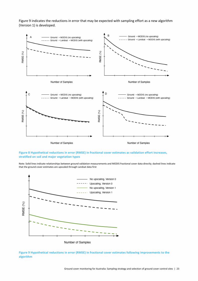
Ground cover monitoring for Australia: Sampling strategy and selection of ground cover control sites | 23
Figure 9 indicates the reductions in error that may be expected with sampling effort as a new algorithm (Version 1) is developed.
Figure 8 Hypothetical reductions in error (RMSE) in fractional cover estimates as validation effort increases, stratified on soil and major vegetation types
Note: Solid lines indicate relationships between ground validation measurements and MODIS fractional cover data directly; dashed lines indicate that the ground cover estimates are upscaled through Landsat data first
Figure 9 Hypothetical reductions in error (RMSE) in fractional cover estimates following improvements to the algorithm
24 | Ground cover monitoring for Australia: Sampling strategy and selection of ground cover control sites
8 Expanding the validation dataset
To reach the number of sampling sites proposed in this report requires additional resources or access to suitable site data funded from other sources. Nationwide measurement efforts that could contribute to the validation of the fractional cover dataset include initiatives of the Terrestrial Ecosystem Research Network (TERN), funded from NCRIS and EIF sources. Of these, the most promising is AusPlots, a subcomponent of the TERN Long-term Australian Multi-scale Plot System (LAMPS) facility. AusPlots is a series of replicated continental-scale surveillance plots implemented in rangelands and forest biomes, to be monitored at low intensity via standardised methods. AusPlots-Rangelands is establishing a network of 100 x 100m plots across the rangelands, building on previous monitoring efforts by state and territory governments, including the Australian Collaborative Rangelands Information System (ACRIS).
Following extensive consultation, a repeatable, quantifiable, and standard sampling method has been devised. 1,000 permanent baseline assessment sites are envisaged in the rangelands with locations stratified on the basis of bioregion, vegetation community type, condition and historical disturbance. The specific location of each plot is ultimately determined in the field.
The intention is to sample the plots once to three times per decade (though only once under NCRIS/EIF funding). Parameters measured include plant taxonomy, vegetation structure, Leaf Area Index, cover, soil parameters, plant genetics, spatial patterning and a measure of homogeneity. These measurements are achieved by a combination of point and transect measures across the plots (B. Sparrow, pers. comm.).
Stratification of the plot locations is based on different criteria than those identified as high priority in this report. A different sampling approach to the SLATS method has also been adopted. Nevertheless, the AusPlots dataset may have considerable value for fractional cover product validation in providing a complementary dataset with additional spatial coverage across the rangelands. Moreover, the appropriateness of each site to MODIS scale validation can be assessed on the basis of a site homogeneity measure. The low sampling intensity will not, however, meet the shorter-term needs for temporal resolution data.
Other TERN initiatives of relevance include:
• Long-Term Ecological Research Network, designed to continue measurements at a core set of existing extensive plot networks or plot transects in key national ecosystems and biomes. Most sites are networks of long archives of plots of variable size, but the AusPlots measurement method will be adopted. This includes estimates of the relative proportions of ground cover.
• TERN AusCover, the primary aim of which is to provide Australian-wide biophysical map products and remote sensing data time-series, but for which field calibration and validation effort is included. Validation will be targeted at up to seven intensive sites (5 x 5 km) covering a range of key biomes, selected for homogeneity, for intensive airborne hyperspectral and lidar studies, and combined with intensive field measurement programs. As such, sampling sites will be few and less concentrated in the rangelands, but will provide data to assess accuracy of fractional cover estimation at a range of scales.
Ground cover monitoring for Australia: Sampling strategy and selection of ground cover control sites | 25
9 Conclusions and recommendations
From the Expert Workshop’s recommendations a sampling strategy to address validation of the fractional cover product is proposed. This aims to validate the MODIS fractional cover product beyond the very limited validation presented in Guerschman et al. (2009). Validation is critical to establish a) confidence in the reliability of the data for use in erosion models, b) highlight areas of low confidence (high error) as useful guidance for algorithm improvement, and c) reliability in monitoring the fractional cover components. In addition to providing inputs to the CEMSYS and SedNet models, the fractional cover product also has potential to track trends in ground cover for land managers. For on-ground decision making reliability of the cover estimates is important.
In the absence of existing validation data, the sampling scheme addresses statistical rigour to achieve confidence in the fractional cover data. It acknowledges the practical challenges in achieving validation of the dataset at continental scale. A stratified sampling approach at 1500 sites is proposed (Figure 3, Tables 1–3) with samples distributed systematically across the targeted areas, focused on areas where accurate cover data is most urgent to inform wind and water erosion studies (across the rangelands and broadacre croplands). It is further focused on grass and shrubland cover types and high priority soils (black, red, gibber and bright).
During year 1 (2010–2011), existing Queensland (~500 sites) and NSW (~30 sites) field estimates of ground cover, obtained using the SLATS method, will be used to perform an initial analysis of the MODIS fractional cover product stratified by soil colour/type, and type and amount of vegetation cover/structure. The output of this analysis, performed by CSIRO Land and Water (Guerschman et al. 2012), will be a preliminary identification of areas where the fractional cover algorithm performs well and less well and allow initial estimates of variability. Consistency in the results across the two states can be assessed and to a certain extent temporal variation. Results will further inform the development of the sampling strategy in subsequent years (2 and 3; 2011–2013) during annual review, for both further validation and algorithm improvement.
Current resourcing may not support sufficient field sampling visits to adequately validate the fractional cover product. Further resources are required and additional TERN-funded surveillance (AusPlots) data could be incorporated. Resourcing is also required for annual review and analysis so the sampling strategy can be adaptively implemented to focus effort on prioritised information needs.
In this study rigour is addressed by consistency, encapsulating:
• a standard methodology for the identification of priority areas for site visits • guidance to field teams on the selection of specific sites to sample • a standard methodology for acquiring field data by the state-based validation teams, including consistent
training in the method and common guidelines • refinement of the sampling effort after annual review as new validation information becomes available • identifying a statistical methodology to better estimate the number of samples potentially required as
field validation data is acquired.
The methodology is independent of both ground cover algorithm and specific satellite sensor. The validation methodology recommends:
• sampling effort is distributed systematically across priority areas in the rangelands and broadacre cropping following the 8 principles in Section 6.1
• in the absence of core knowledge, a reasoned, credible initial number of sampling sites is 1500 sites; their distribution across states and territories and priority soil types is presented in Tables 1 to 3

26 | Ground cover monitoring for Australia: Sampling strategy and selection of ground cover control sites
• an annual analysis of the acquired validation data to confirm existing sites, assess the validity of the assumption of 1500 sites, and assess the impact of sampling effort on overall product uncertainty; Section 7 outlines the main steps involved in this analysis
• higher spatial resolution satellite data (e.g. Landsat) is used in future analysis to understand errors arising from scaling differences between on-ground measurements and the MODIS data.
Ground cover monitoring for Australia: Sampling strategy and selection of ground cover control sites | 27
Appendix A The fractional cover product – basis of the algorithm
The approach of Guerschman et al. (2009) is based on the feature-space plot of the Normalised Difference Vegetation Index (NDVI) versus the Cellulose Absorption Index (CAI). ‘Pure’ end-members for photosynthetic (green) vegetation, non-photosynthetic (brown) vegetation and bare soil group at the apices of a triangle of the dispersion in pixel space (Apx Figure A.1). A pixel is assigned cover values in proportions of these three fractions on the basis of where it lies in the pixel space.
The two indices used to derive the cover plots in Apx Figure A.1 are:
NDVI = (ρ800- ρ600) / (ρ800+ ρ600) (2)
CAI = 0.5·(ρ2000+ ρ2200) - ρ2100 (3)
where ρ### represents reflectances measured in the satellite bands with centre wavelengths as specified (in nm).
The product was initially developed based on hyperspectral field data obtained in the northern part of the Northern Territory in July 2005. It was validated with the use of 3 Hyperion hyperspectral images obtained at different times of the same year for the same region (Apx Figure A.1b).
To adapt the index to provide fractional cover estimates across Australia using MODIS/Terra satellite data (atmospherically corrected, nadir BRDF-adjusted reflectance data – MOD43B4 Collection 4 data) a band ratio based on MODIS SWIR bands 2 and 3 was used as a proxy for the CAI. This gives a compressed triangle for the MODIS product (Apx Figure A.1c). Nevertheless, the resulting product provides continental fractional cover estimates at 16-day intervals at 500 metre resolution (example, Apx Figure A.2), from 2000 to the present day.
Quality flags are used to highlight the extent the unmixing process into the three cover components is constrained. The current flags used are:
• 0 – pixel processed normally, unmixing ‘unconstrained’ • 1 – unmixing partially constrained, fractional cover estimated • 2 – unmixing constrained, fractional cover not calculated (fractional cover 0%; pixel lies outside the
triangle) • 255 – MODIS NBAR data not available, for example due to cloud.
Further details about the algorithm and its development are in Guerschman et al. (2009).

28 | Ground cover monitoring for Australia: Sampling strategy and selection of ground cover control sites
a b c
Apx Figure A.1 Theoretical basis of the Guerschman et al. (2009) algorithm (a), application to Hyperion data (b) and resultant MODIS adaptation using SWIR bands 2 and 3 (c).
Apx Figure A.2 Example of the MODIS fractional cover continental product
Note: BS, bare soil; PV, photosynthetic vegetation; NPV, non-photosynthetic vegetation
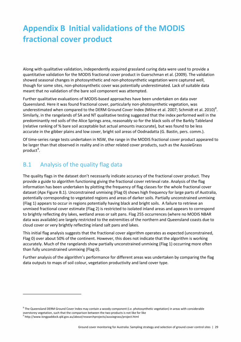
Ground cover monitoring for Australia: Sampling strategy and selection of ground cover control sites | 29
Appendix B Initial validations of the MODIS fractional cover product
Along with qualitative validation, independently acquired grassland curing data were used to provide a quantitative validation for the MODIS fractional cover product in Guerschman et al. (2009). The validation showed seasonal changes in photosynthetic and non-photosynthetic vegetation were captured well, though for some sites, non-photosynthetic cover was potentially underestimated. Lack of suitable data meant that no validation of the bare soil component was attempted.
Further qualitative evaluations of MODIS-based approaches have been undertaken on data over Queensland. Here it was found fractional cover, particularly non-photosynthetic vegetation, was underestimated when compared to the DERM Ground Cover Index (Milne et al. 2007; Schmidt et al. 2010)8
Of time-series range tests undertaken in NSW, the range in the MODIS fractional cover product appeared to be larger than that observed in reality and in other related cover products, such as the AussieGrass product
. Similarly, in the rangelands of SA and NT qualitative testing suggested that the index performed well in the predominantly red soils of the Alice Springs area, reasonably so for the black soils of the Barkly Tableland (relative ranking of % bare soil acceptable but actual amounts inaccurate), but was found to be less accurate in the gibber plains and low cover, bright soil areas of Oodnadatta (G. Bastin, pers. comm.).
9
B.1 Analysis of the quality flag data
.
The quality flags in the dataset don’t necessarily indicate accuracy of the fractional cover product. They provide a guide to algorithm functioning giving the fractional cover retrieval rate. Analysis of the flag information has been undertaken by plotting the frequency of flag classes for the whole fractional cover dataset (Apx Figure B.1). Unconstrained unmixing (Flag 0) shows high frequency for large parts of Australia, potentially corresponding to vegetated regions and areas of darker soils. Partially unconstrained unmixing (Flag 1) appears to occur in regions potentially having black and bright soils. A failure to retrieve an unmixed fractional cover estimate (Flag 2) is restricted to isolated inland areas and appears to correspond to brightly reflecting dry lakes, wetland areas or salt pans. Flag 255 occurrences (where no MODIS NBAR data was available) are largely restricted to the extremities of the northern and Queensland coasts due to cloud cover or very brightly reflecting inland salt pans and lakes.
This initial flag analysis suggests that the fractional cover algorithm operates as expected (unconstrained, Flag 0) over about 50% of the continent. However, this does not indicate that the algorithm is working accurately. Much of the rangelands show partially unconstrained unmixing (Flag 1) occurring more often than fully unconstrained unmixing (Flag 0).
Further analysis of the algorithm’s performance for different areas was undertaken by comparing the flag data outputs to maps of soil colour, vegetation productivity and land cover type.
8 The Queensland DERM Ground Cover Index may contain a woody component (i.e. photosynthetic vegetation) in areas with considerable overstorey vegetation, such that the comparison between the two products is not like for like 9 http://www.longpaddock.qld.gov.au/about/researchprojects/aussiegrass/project.html

30 | Ground cover monitoring for Australia: Sampling strategy and selection of ground cover control sites
Apx Figure B.1 Flag class frequencies for the MODIS fractional cover product (for 2000–08).
B.2 Flag analysis by soil colour
Qualitative evidence suggests that the soil surface’s spectral colour influences the fractional cover result (G. Bastin, pers. comm.). To discover possible associations between the flag class data and some of the principal soils in Australian rangelands, areas where the flag class frequencies exceed 80% were overlaid on the derived 1:2.5 million scale soil colour map (Figure 3e). The results are presented in Apx Table B.1. The assumption is that if the frequency of Flag 1, 2 and 255 is higher than the national percentage then this indicates an association between the flag classes and soil colour.

Ground cover monitoring for Australia: Sampling strategy and selection of ground cover control sites | 31
Apx-Table B.1 Analysis of soil colour for areas with greater than 80% of each flag class
FLAG CLASS
SOIL COLOUR 0 1 2 255 TOTAL
Gibber 4% 60% 34% 3% 100%
Bright 47% 32% 14% 7% 100%
Red 47% 36% 14% 3% 100%
Black 42% 40% 13% 5% 100%
Other 45% 30% 18% 8% 100%
Flag 0, pixel processed normally, unmixing unconstrained; Flag 1, unmixing partially constrained, fractional cover estimated; Flag 2, unmixing constrained, fractional cover not calculated (fractional cover 0%); Flag 255, MODIS NBAR data not available e.g. cloud
Associations appear to be acute in areas of sparse vegetation as opposed to areas where ground cover is higher. Flag 255 had a fairly low frequency of occurrence (less than 7%). The analysis suggests that gibber in particular is associated with very high frequencies of Flag 1 and 2, with 60% of the flag area falling in the high frequency zone for Flag 1. Low Flag 0 percentages (where algorithm was successfully applied) for gibber indicate that the algorithm consistently failed over gibber areas. For the remaining soil colours, most of the data falls in Flag 0 and 1. This indicates that more than 75% of the data have been successfully processed using the fractional cover algorithm.
B.3 Flag analysis by vegetation productivity
The flag data were compared with vegetation productivity data compiled from MODIS Enhanced Vegetation Index (EVI, or greenness) data for 2000–0810
This analysis showed that the algorithm ‘worked’ most frequently (Flag 0) in areas of high productivity (high EVI). Low and medium values of EVI had higher proportions of Flag 1. Low values of EVI had a higher proportion of Flag 2 compared with medium and high values of EVI. This suggests that the algorithm is more prone to error in areas of low to medium productivity, such as the rangelands.
(Apx Figure B.2). The intensive land use zone falls within the high EVI class, whilst the low EVI class delineates the deserts and sparse shrublands and hummock grasslands. The frequency of EVI classes was compared to flag classes in Table B.2.
Apx-Table B.2 Analysis of frequency of occurrence of flag values as a percentage of Enhanced Vegetation Index values
FLAG CLASS
SOIL COLOUR 0 1 2 255 TOTAL
Low 15% 52% 27% 6% 100%
Medium 38% 47% 10% 5% 100%
High 56% 20% 15% 9% 100%
EVI classes: Low (<0.13); Medium (0.13–0.19); High (0.19–0.72) based on an equal area distribution
10 modis.gsfc.nasa.gov/data/dataprod/dataproducts.php?MOD_NUMBER=13;
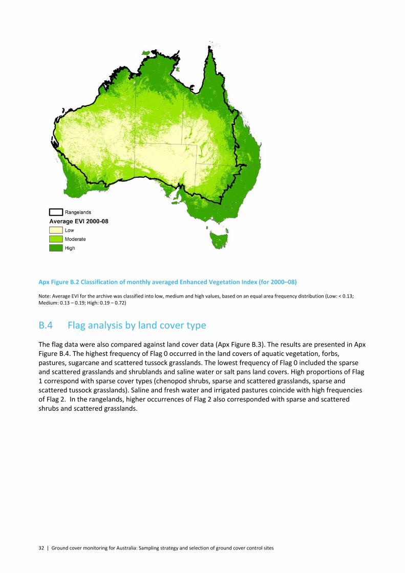
32 | Ground cover monitoring for Australia: Sampling strategy and selection of ground cover control sites
Apx Figure B.2 Classification of monthly averaged Enhanced Vegetation Index (for 2000–08)
Note: Average EVI for the archive was classified into low, medium and high values, based on an equal area frequency distribution (Low: < 0.13; Medium: 0.13 – 0.19; High: 0.19 – 0.72)
B.4 Flag analysis by land cover type
The flag data were also compared against land cover data (Apx Figure B.3). The results are presented in Apx Figure B.4. The highest frequency of Flag 0 occurred in the land covers of aquatic vegetation, forbs, pastures, sugarcane and scattered tussock grasslands. The lowest frequency of Flag 0 included the sparse and scattered grasslands and shrublands and saline water or salt pans land covers. High proportions of Flag 1 correspond with sparse cover types (chenopod shrubs, sparse and scattered grasslands, sparse and scattered tussock grasslands). Saline and fresh water and irrigated pastures coincide with high frequencies of Flag 2. In the rangelands, higher occurrences of Flag 2 also corresponded with sparse and scattered shrubs and scattered grasslands.

Ground cover monitoring for Australia: Sampling strategy and selection of ground cover control sites | 33
Apx Figure B.3 Classification of land cover
Source: Geoscience Australia

34 | Ground cover monitoring for Australia: Sampling strategy and selection of ground cover control sites
Apx Figure B.4 Flag class frequencies by land cover classes
Note: Flag 0, pixel processed normally, unmixing unconstrained; Flag 1, unmixing partially constrained, fractional cover estimated; Flag 2, unmixing constrained, fractional cover not calculated (fractional cover 0%); Flag 255, MODIS NBAR data not available e.g. cloud
Ground cover monitoring for Australia: Sampling strategy and selection of ground cover control sites | 35
B.5 Seasonal quality flag analysis
An analysis of the occurrences of quality flags at different times of the year assists field site selection and timing of field data acquisition. The mean frequency for each season from autumn 2000 to summer 2011 was calculated for each of the flags.
Only the data for Flag 0 (Apx Figure B.5) and Flag 1 (Apx Figure B.6) are presented as these are most important, in terms of the rangelands, as identified above. High Flag 0 frequencies are found throughout the year, particularly for those areas with moderate or evenly spread rainfall. Unconstrained unmixing is more widespread in autumn and winter and least often in summer. The lowest occurrences of Flag 1 (partially unconstrained mixing) were in autumn and winter and most often in the rangelands in spring and summer (Apx Figure B.6).
Apx Figure B.5 Seasonal analysis of Flag 0 occurrences indicating unconstrained unmixing

36 | Ground cover monitoring for Australia: Sampling strategy and selection of ground cover control sites
Apx Figure B.6 Seasonal analysis of Flag 1 occurrences indicating partially unconstrained unmixing
B.6 Summary of the quality flag analysis
The flag analysis showed fractional cover processing was most successful (Flag 0) for all soils except gibber, but there were also significant proportions of Flag 1 (>30%) and Flag 2 (>13%) in areas of bright, red and black soils (Apx Table B.1). The algorithm was also most successful for areas with high greenness and land covers such as cropping, woodlands and aquatic vegetation. The combination of these soils and land-cover types is more likely to be found in the intensive land use zone.
The fractional cover analysis performed poorly, giving a higher proportion of occurrences of Flag 1 and 2, in rangeland areas where low greenness, gibber soils and sparse and scattered vegetation were found. This suggests that validation sites in the rangelands are a priority to improve the fractional cover processing.
Spring and summer had higher occurrences of processing errors, particularly in the rangelands. There were fewer occurrences of processing errors in autumn and winter. This supports targeting site visits initially, where practical, in spring and summer where validation will potentially most quickly lead to improved algorithm accuracy and fewer processing errors.
Ground cover monitoring for Australia: Sampling strategy and selection of ground cover control sites | 37
B.7 Conclusions on initial validation
Much of the validation undertaken on the MODIS fractional cover product so far is qualitative giving no quantitative indication of the product’s accuracy.
There is reasonable qualitative agreement with knowledge in some areas, and a strong association between algorithm retrieval performance and soil type. Whilst the analysis of the flag data is not a validation per se, it does highlight the poor fractional cover retrieval over gibber soils and to a lesser extent for red and black soils. Poor algorithm performance over these soils may reflect that the algorithm’s end-members were based on transect data from mainly seasonally green, tropical savannah in the Northern Territory. However, soil colour and moisture content can also have significant impacts on soil reflectance and thus on measures of vegetation greenness derived from remotely sensed reflectance (Huete et al. 1985, Liu et al. 2002, Lobell and Asner 2002). Soil moisture variations may also affect both retrieval and accuracy of the fractional cover algorithm (Bastin et al. 2006).
The algorithm also appears to be more prone to errors in areas of sparse vegetation typical of the rangelands. This may be a result of the confounding influences of soil colour and moisture status, which would have a greater influence in more sparsely, vegetated areas. Similarly, in a simple index such as this, the spectral similarities between senescent cover and bright soils (Asner and Heidebrecht 2003) and between shade and dark soil (Okin et al. 2001) may also cause the algorithm to fail.
In some areas seasonal variation in estimated ground cover appears to be realistic with perhaps some over or under estimation at the extremes of ground cover.
There is a clear need for significant further quantitative validation of the MODIS fractional cover product. Confidence in the data needs to be established, as does further understanding of the regions and conditions under which errors may occur in fractional cover estimates and which might aid the further development of the product.
Further effort aimed at quantitative validation needs to take into account influences on the fractional cover algorithm retrieval and accuracy brought about by:
• differences in soil colour • variations in soil moisture content • vegetation amount, in particular the algorithms accuracy in low vegetation covers where risk of erosion
may be highest.
The validation effort should initially concentrate on the rangelands in regions of varying soil colour background and vegetation cover.

38 | Ground cover monitoring for Australia: Sampling strategy and selection of ground cover control sites
Appendix C Expert Workshop attendees
GROUND COVER MONITORING FOR AUSTRALIA
Expert Workshop on Sampling Strategy and Selection of Ground Cover Control Sites
Tuesday 17th August and Wednesday 18th of August 2010
Christian Lab Conference Room, CSIRO Land and Water, Christian Laboratories, Black Mountain, Canberra
Workshop attendees
Bob Karfs Department of Employment, Economic Development and Innovation, Queensland11
Gary Bastin
CSIRO Ecosystem Sciences
Glenn Stone CSIRO Mathematics, Informatics and Statistics
Jane Stewart Australian Bureau of Agricultural and Resource Economics and Sciences
Jeff Thompson Department of Geography, Australian Defence Force Academy
John Leys Department of Environment, Climate Change and Water, New South Wales12
Lucy Randall
Australian Bureau of Agricultural and Resource Economics and Sciences
Michele Barson Department of Agriculture Fisheries and Forestry
Peter Scarth Department of Environment and Resource Management, Queensland13
Simon Barry
CSIRO Mathematics, Informatics and Statistics
Tim Danaher Department of Environment, Climate Change and Water, New South Wales
Tim Malthus CSIRO Land and Water
Tim McVicar CSIRO Land and Water
Vivienne Bordas Australian Bureau of Agricultural and Resource Economics and Sciences
11 Now Department of Agriculture, Fisheries and Forestry, Queensland 12 Now Department of Premier and Cabinet, Office of Environment and Heritage, New South Wales 13 Now Department of Science, Information Technology, Innovation and the Arts, Queensland

Ground cover monitoring for Australia: Sampling strategy and selection of ground cover control sites | 39
Appendix D Expert Workshop agenda
GROUND COVER MONITORING FOR AUSTRALIA
Expert Workshop on Sampling Strategy and Selection of Ground Cover Control Sites
Tuesday 17th August and Wednesday 18th of August 2010
Christian Lab Conference Room, CSIRO Land and Water, Christian Laboratories, Black Mountain, Canberra
Agenda
Day 1 – Tuesday 17th 09:00–17:30
1. Welcome – introduction, aims and outputs of the workshop (Michele Barson / Jane Stewart)
2. Introduction to the fractional cover product and project (Tim Malthus)
3. Quality issues with the fractional cover product (Lucy Randall)
4. Approaches to site selection
• multi criteria (Simon Barry) • index based (Tim McVicar)
5. Introduction to the MCAS toolbox and datasets (Lucy Randall)
6. Discussion to identify initial issues of concern
(12:30 to 13:30 Lunch)
7. Interactive session (Simon Barry)
Prioritisation of sampling sites using MCAS, aiming to:
• identify the top 10 data layers to be used in prioritisation • determine if we can reach a consensus on key priorities • explore different permutations in site selection • identify what potential data layers/information is still missing.
Day 2 – Wednesday 18th 09:00–12:30
8. Analysis of yesterday’s outcomes, Summing up commonalities identified (TBD)
9. Establishment of a general sampling prioritisation map (TBD)
10. Next steps – discussion on specific site selection and sampling protocols (TBD). For example:
• What accuracy are we aiming for? • How many sites? • How frequently will we sample? • When do we have enough sites?
11. Conclusions and close
40 | Ground cover monitoring for Australia: Sampling strategy and selection of ground cover control sites
Appendix E Sampling protocol for 2010–201114
E.1 Background
A national field data collection campaign commenced in 2010–11 to validate the MODIS-derived vegetation fractional cover product developed by Guerschman et al. (2009). To prioritise where to locate sites for this campaign a sampling protocol was developed based on expert advice from a sampling strategy workshop held on 17 and 18 August 2010.
Site selection for measurement of fractional ground cover for site data collected in 2010 and 2011 was stratified based on:
• soil colour—to interpret reflectance of bare soil • agricultural land uses—focused on rangelands and extensive grazing systems (excluding conservation or
indigenous protected areas) • non-treed areas and open woodlands—where tree canopy cover was less than 20 per cent.
Partner agencies were trained in site description and measurement of fractional cover based on Queensland DERM’s Statewide Landcover and Trees Study methodology. This document provides protocols which were used for site selection only. Refer to the field manual (Muir et al. 2011) for further details on establishing, describing and measuring a site.
Fractional ground cover has been considered as three components:
• photosynthetic vegetation (PV)—green attached leaf • non-photosynthetic vegetation (NPV)—dry attached leaf and litter • bare soil (BS)—crust, disturbed, rock and cryptogam.
E.2 Steps
The sampling process consisted of five steps that can be briefly summarised as:
• Step 1: Partner agencies selected sites according to cover and soil colour • Step 2: Partner agencies calculated the proportion of field sites for each soil colour • Step 3: Partner agencies selected an image tile using sampling.mxd • Step 4: Partner agencies selected a cloud-free image from the GloVis website • Step 5: Partner agencies collected site data based on field manual.
E.2.1 STEP 1
Partner agencies selected sites that represented the:
• soil colours of interest (Apx Table E.1, Apx Table E.2 and Apx Figure E.1) • range of fractional cover, given seasonal conditions:
– low brown (NPV) or green (PV) cover – high green cover – high brown cover.
14 Extract from Stewart et al. (2012)
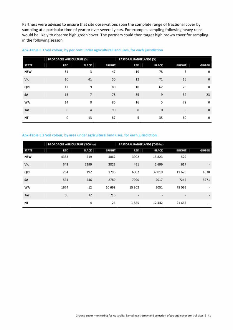
Ground cover monitoring for Australia: Sampling strategy and selection of ground cover control sites | 41
Partners were advised to ensure that site observations span the complete range of fractional cover by sampling at a particular time of year or over several years. For example, sampling following heavy rains would be likely to observe high green cover. The partners could then target high brown cover for sampling in the following season.
Apx-Table E.1 Soil colour, by per cent under agricultural land uses, for each jurisdiction
BROADACRE AGRICULTURE (%) PASTORAL RANGELANDS (%)
STATE RED BLACK BRIGHT RED BLACK BRIGHT GIBBER
NSW 51 3 47 19 78 3 0
Vic 10 41 50 12 71 16 0
Qld 12 9 80 10 62 20 8
SA 15 7 78 35 9 32 23
WA 14 0 86 16 5 79 0
Tas 6 4 90 0 0 0 0
NT 0 13 87 5 35 60 0
Apx-Table E.2 Soil colour, by area under agricultural land uses, for each jurisdiction
BROADACRE AGRICULTURE (‘000 ha) PASTORAL RANGELANDS (‘000 ha)
STATE RED BLACK BRIGHT RED BLACK BRIGHT GIBBER
NSW 4383 219 4062 3902 15 823 529 -
Vic 543 2299 2825 461 2 699 617 -
Qld 264 192 1796 6002 37 019 11 670 4638
SA 534 246 2789 7990 2017 7245 5271
WA 1674 12 10 698 15 302 5051 75 096 -
Tas 50 32 716 - - - -
NT - 4 25 1 885 12 442 21 653 -

42 | Ground cover monitoring for Australia: Sampling strategy and selection of ground cover control sites
Apx Figure E.1 Soil colour
E.2.2 STEP 2
Partner agencies calculated the proportion of field sites for each soil colour based on the amount of each soil colour estimated to be under broadacre agriculture and pastoral rangelands. Partner agencies multiplied the total number of sites to be collected by the soil colour percentages in Apx Table E. 1.
E.2.3 STEP 3
Partner agencies selected an image tile using the spatial data layers provided by ABARES in an ArcMap GIS project file called sampling.mxd.
• Soil colour based on the Digital Atlas of Australian Soils15, interpreted into colours using Northcote (1979) and then refined by expert opinion. Gibber targets derived using land systems data for South Australia, IBRA sub-regions16
– red (Code 3)
and expert opinion.
– black (Code 5) – bright (Code 2) – gibber (Code 1) – other (Code 0) was not identified as a priority.
15 http://adl.brs.gov.au/anrdl/metadata_files/pa_daaslr9abd_00111a01.xml 16 http://www.environment.gov.au/metadataexplorer/full_metadata.jsp?docId=%7BAC901094-DA0D-4BF2-B957-3202AA189258%7D&loggedIn=false

Ground cover monitoring for Australia: Sampling strategy and selection of ground cover control sites | 43
• Land use/cover
– Tree cover mask included:
- no tree cover (Code 0) - forest/plantation (Code 1) based on Forests of Australia 200817
– Agricultural mask derived from Catchment scale land use of Australia–Update March 2010
. 18
- grazing of native pastures, modified pastures and cropping (Code 0)
. Classified into:
- non-agricultural (Code 1).
– Rangeland boundary (Bastin et al. 2008) included:
- rangelands (Code 0) - non-rangelands (Code 2) from rangeland boundary.
– Site accessibility included:
- distance from field team—states created using location and straight-line distance - distance from all roads—included in ArcMap project - existing sites—included in ArcMap project - tenure—included in ArcMap project - Landsat tiles—included in ArcMap project.
• Other data—to ensure that the imagery represents the field conditions:
– image was to be within one month of field data collection – sites where there has been rainfall subsequent to the image were avoided – sites where there have been recent fires were avoided – collection was to be coordinated with roadside erosion surveys, if applicable.
E.2.4 STEP 4
Partner agencies selected a cloud-free image from the United States Geological Survey Global Visualization Viewer19
• Sites were to be away from soil colour edges and at least 500 metres from a change in cover. This is to ensure sites are homogenous at the MODIS fractional cover scale.
. Landsat 5 TM imagery was preferred. Where Landsat 7 ETM+ imagery was collected, only the centre portion of the image could be used. Partners used the imagery to select at least five sites based on the following criteria:
• Existing sites were used, where feasible, to decrease time and cost. • Sites were to be accessible by road—as included in ArcMap project. • Property and landholder information was to be identified using existing state datasets.
17 http://adl.brs.gov.au/anrdl/metadata_files/pa_foraug9abll0062008_11a.xml 18 http://adl.brs.gov.au/anrdl/metadata_files/pa_luausr9abll07611a00.xml 19 http://glovis.usgs.gov/
44 | Ground cover monitoring for Australia: Sampling strategy and selection of ground cover control sites
E.2.5 STEP 5
Partner agencies collected site data based on field manual (Muir et al. 2011) to include:
• location—latitude and longitude • date of field collection • field attributes • fractional cover data.
E.3 Field campaign checklist
Partner agencies were responsible for:
• identifying Landsat scene (path/row) for field data collection • identifying property and landholder, contacting landholder and obtaining permission in principle to
sample their property; if cropping site, checking growth phase or timing of land management practice • checking cloud-free Landsat imagery available • sending details of Landsat scene (sensor L5 path/row) and date (dd/mm/yyyy) to ABARES • keeping a watching brief for subsequent fires and/or rainfall; and changing sites or cancelling field work if
these occurred between image collection and the scheduled field visit • organising staff availability, vehicles and equipment, accommodation and other needs • confirming field dates with landholders • collecting field data, photographs, filling in field data forms; sending data to ABARES.

Ground cover monitoring for Australia: Sampling strategy and selection of ground cover control sites | 45
Shortened forms and glossary
ABARES Australian Bureau of Agricultural and Resource Economics and Sciences
BRDF Bi-directional Reflectance Distribution Function
BS Bare Soil
CAI Cellulose Absorption Index
Calibration The process of quantitatively defining the system responses to known, controlled signal inputs.
CEMSYS Computational Environmental Management System model
DERM Department of Environment and Resource Management, Queensland
EIF Education Investment Fund
EVI Enhanced Vegetation Index
Foliage Projected Cover The proportion of the ground covered by the vertical projection of the vegetation.
IBRA Interim Biogeographic Regionalisation for Australia
MODIS MODerate-resolution Imaging Spectroradiometer
Nadir The satellite viewing angle directly downward
NBAR Nadir BRDF-Adjusted Reflectance
NCAS National Carbon Accounting System
NCRIS National Collaborative Research Infrastructure Strategy
NDVI Normalised Difference Vegetation Index
NPV Non-Photosynthetic Vegetation
PV Photosynthetic Vegetation
Qualitative Validation For remotely sensed fractional cover, is testing that the data can mimic field observations and the expectations or experience of local experts.
Quantitative Validation For remotely sensed fractional cover, is testing that the data can accurately estimate all or some of the quantifiable fractions of vegetation cover made from previous or contemporary observations in the field, such that levels of accuracy can be derived.
RMSE Root Mean Square Error
SedNet Sediment Network modelling software
SLATS Statewide Land Cover And Trees Study
SWIR Short-wavelength infrared (0.7 to 300 µm)
TERN Terrestrial Ecosystem Research Network
Validation The process of assessing, by independent means, the quality of the data products derived from the system outputs.

46 | Ground cover monitoring for Australia: Sampling strategy and selection of ground cover control sites
References
ANRA (2009) Australian Natural Resources Atlas, Natural Resource Topics: Soils. <http://www.anra.gov.au/topics/soils/index.html>
Asner GP and Heidebrecht KB (2003) Imaging spectroscopy for desertification studies: comparing AVIRIS and EO-1 Hyperion in Argentina drylands. IEEE Transactions on Geoscience and Remote Sensing, 41:1283−1296.
Barson M, Mewett J and Paplinska J (2012) Land management practice trends in Australia's broadacre cropping industries. Caring for our Country Sustainable Practices Fact Sheet 3. Department of Agriculture, Fisheries and Forestry, Canberra. <http://www.daff.gov.au/__data/assets/pdf_file/0006/2148711/national-factsheet-farm-practices-broadacre.pdf >
Bastin G and ACRIS (Australian Collaborative Rangelands Information System) Management Committee (2008) Rangelands 2008 – Taking the pulse. National Land and Water Resources Audit, Canberra. <http://www.environment.gov.au/land/publications/acris/report08.html>
Bastin G, James C, Chewings V and Brook A (2006) Wool producers with remote control: New tools for whole of property management. Final report for Land, Water and Wool Funded Project CSE 27. <http://lwa.gov.au/products/pk071421>
Furby S (2002) Land cover change: specification for remote sensing analysis. National Carbon Accounting System technical report No. 9. Australian Greenhouse Office. <http://pandora.nla.gov.au/tep/23322>
Guerschman JP, Hill MJ, Renzullo LJ, Barrett DJ, Marks AS and Botha EJ (2009) Estimating fractional cover of photosynthetic vegetation, non-photosynthetic vegetation and bare soil in the Australian tropical savanna region upscaling the EO-1 Hyperion and MODIS sensors. Remote Sensing of Environment, 113:928–945.
Guerschman JP, Oyarzabal M, Malthus TJ, McVicar TR, Byrne G, Randall LA and Stewart JB (2012) Evaluation of the MODIS-based vegetation fractional cover product. Report No. EP11631, CSIRO, Canberra. <http://www.clw.csiro.au/publications/science/2012/SAF-MODIS-fractional-cover.pdf>
Hairsine PB, Barson M, Randall L and Wilkinson SN (2009) The 2009 expert panel process in support of the spatial targeting of the Caring for Our Country (C4OC) investment concerning hillslope erosion by water. CSIRO Land and Water Science Report 09/45. <http://www.clw.csiro.au/publications/science/2009/sr45-09.pdf>
Huete AR, Jackson RD and Post DF (1985) Spectral response of a plant canopy with different soil backgrounds. Remote Sensing of Environment, 17:37–53.
Lesslie RG, Hill MJ, Hill P, Cresswell HP and Dawson S (2008) The application of a simple spatial multi-criteria analysis shell to natural resource management decision making. In: Pettit C, Cartwright W, Bishop I, Lowell K, Pullar D and Duncan D (Eds), Landscape Analysis and Visualisation: Spatial Models for Natural Resource Management and Planning, Springer, Berlin, pp 73–96.
Liu W, Baret F, Gu X, Tong Q, Zheng L and Zhang B (2002) Relating soil surface moisture to reflectance. Remote Sensing of Environment, 81:238–246.
Liu YY, Parinussa RM, Dorigo WA, De Jeu RAM, Wagner W, Van Dijk AIJM, McCabe MF and Evans JP (2011) Developing an improved soil moisture dataset by blending passive and active microwave satellite-based retrievals. Hydrology and Earth Systems Science, 15:425–436.
Lobell DB and Asner GP (2002) Moisture effects on soil reflectance. Soil Science Society of America Journal, 66:722–727.

Ground cover monitoring for Australia: Sampling strategy and selection of ground cover control sites | 47
Lowell K, Woodgate P, Jones S and Richards GP (2003) Continuous improvement of the NCAS land cover change mapping. National Carbon Accounting System technical report no. 39. Australian Greenhouse Office. <http://pandora.nla.gov.au/tep/23322>
Lymburner L, Tan P, Mueller N, Thackway R, Lewis A, Thankappan M, Randall L, Islam A and Senarath U (2011) The national dynamic land cover dataset. Record 2011/31, Geoscience Australia, Symonston, ACT. GeoCat # 71069. <https://www.ga.gov.au/products/servlet/controller?event=GEOCAT_DETAILS&catno=71069>
McKeon G, Hall W, Henry B, Stone G and Watson I (2004) Pasture degradation and recovery in Australia's rangelands: Learning from history. Department of Natural Resources, Mines and Energy, Queensland Government. May 2004Report No. QNRME04130. <http://www.longpaddock.qld.gov.au/about/publications/learningfromhistory/index.html>
Milne J, Danaher T, Scarth P, Carter J, Armston J, Henry B, Cronin N, Hassett R, Stone G, Williams P, Denham R and Byrne M (2007) Evaluation of MODIS for groundcover and biomass/feed availability estimates in tropical savannah systems. Meat and Livestock Australia, North Sydney. 114 pp.
Montreal Process Implementation Group for Australia (2008) Australia’s State of the Forests Report 2008. Bureau of Rural Sciences, Canberra. <http://adl.brs.gov.au/forestsaustralia/_pubs/sofr2008reduced.pdf>
Muir J, Schmidt M, Tindall D, Trevithick R, Scarth P and Stewart JB (2011) Field measurement of fractional ground cover: a technical handbook supporting ground cover monitoring for Australia. Prepared by the Queensland Department of Environment and Resource Management for the Australian Bureau of Agricultural and Resource Economics and Sciences, Canberra. <http://adl.brs.gov.au/data/warehouse/pe_hbgcm9abll07701/HndbkGrndCovMontring2011_1.0.0_HR.pdf>
Northcote KH (1979) A factual key for the recognition of Australian soils, 4th Edition. Rellim Technical Publications, Glenside, South Australia.
Northcote KH, Beckmann GG, Bettenay E, Churchward HM. Van Dijk DC, Dimmock GM, Hubble GD, Isbell RF, McArthur WM, Murtha GG, Nicolls KD, Paton TR, Thompson CH. Webb AA and Wright MJ (1960–1968) Atlas of Australian Soils. CSIRO and Melbourne University Press, Melbourne.
Okin GS, Roberts DA, Murray B and Okin WJ (2001) Practical limits on hyperspectral vegetation discrimination in arid and semiarid environments. Remote Sensing of Environment, 77:212–225.
Scarth P, Byrne M, Danaher T, Henry B, Hassett R, Carter J and Timmers P (2006) State of the paddock: monitoring condition and trend in ground cover across Queensland. The 13th Australasian Remote Sensing and Photogrammetry Conference, Canberra.
Schmidt M, Tindall D, Speller K, Scarth P and Dougall C (2010) Ground cover management practices in cropping and improved pasture grazing systems: ground cover monitoring using remote sensing. Final report to the Bureau of Rural Sciences, State of Queensland, Department of Environment and Resource Management. <http://adl.brs.gov.au/landuse/docs/Groundcover_remotesensing2010.pdf>
Shao Y, Leys J, McTainsh G and Tews K (2007) Numerical simulation of the October 2002 dust event in Australia. Journal of Geophysical Research, 112:1–12.
Stewart JB, Rickards JE, Bordas VM, Randall LA and Thackway RM (2011) Ground cover monitoring for Australia – establishing a coordinated approach to ground cover mapping: Workshop proceedings Canberra 23–24 November 2009. Australian Bureau of Agricultural and Resource Economics and Sciences, Canberra. <http://adl.brs.gov.au/data/warehouse/pe_abares99001799/Groundcover_mapping-workshop_proc_11.pdf>
Stewart JB, Randall LA, Rickards JE and Bordas VM (2012) Ground cover monitoring for Australia: Progress report to June 2011. ABARES Technical report 12.1, Australian Bureau of Agricultural and Resource
48 | Ground cover monitoring for Australia: Sampling strategy and selection of ground cover control sites
Economics and Sciences, Canberra. <http://adl.brs.gov.au/data/warehouse/gcmfap9abll080/GroundCoverMonitoringAust_v.1.0.0.pdf>
Thackway R and Cresswell ID (1995) An interim biogeographic regionalisation for Australia: a framework for setting priorities in the national reserves system cooperative program. Australian Nature Conservation Agency, Canberra.
Wilkinson S, Henderson A, Chen Y and Sherman B (2004) SedNet user guide. Client Report to the Cooperative Research Centre for Catchment Hydrology, CSIRO Land and Water, Canberra. <http://www.toolkit.net.au/Tools/SedNet/documentation>


50 | Ground cover monitoring for Australia: Sampling strategy and selection of ground cover control sites
CONTACT US t 1300 363 400 +61 3 9545 2176 e [email protected] w www.csiro.au
YOUR CSIRO Australia is founding its future on science and innovation. Its national science agency, CSIRO, is a powerhouse of ideas, technologies and skills for building prosperity, growth, health and sustainability. It serves governments, industries, business and communities across the nation.
FOR FURTHER INFORMATION CSIRO Land and Water Dr Tim J Malthus Program Leader and Research Scientist t +61 2 6246 5732 e [email protected] w www.csiro.au/Organisation-Structure/Divisions/Land-and-Water