Ground state of quantum gravity in

dynamical triangulation

Jan Smit

Institute for Theoretical Physics,University of Amsterdam & Utrecht University,

the Netherlands

1

1. Euclidean dynamical triangulation

2. Curvature of emerging space-times

3. Test particles

4. Induced mass in the crumpled phase∗

5. Scaling

6. Conclusion

∗Presenting unpublished (’96) data of work with Bas V. de Bakker

2

Euclidean Dynamical Triangulation (EDT)∗

Simplicial manifold build of equilateral 4-simplices

Ni, i = 0,1, . . . ,4 number of i-simplices

χ = N0 −N1 + N2 −N3 + N4 Euler

χ fixed: only two Ni are independent

∗Weingarten, NPB210[FS6](1982)229; Ambjørn, Jurkiewicz,

PLB278(1992)42; Agishtein, Migdal, MPLA7(1992)1039

3

‘pure gravity’

S =

∫d4x

√g

(2Λ0 −R

16πG0

)

→ −κ2N2 + κ4N4

κ2 =V2

8πG0, κ4 =

Λ0 + 10θV2

8πG0

θ = arccos(1/4) Regge deficit angle

Vi =`i√

i + 1

i!√

2ivolume of i-simplex

` edge length

4

Z =

∫Dg e−S →

Z(κ2, κ4) =∑

Teκ2N2−κ4N4

=∑

N4

e−κ4N4Z(κ2, N4)

Z(κ2, N4) =∑

T (N4)

eκ2N2

∼ (N4)γ−3 eκc

4N4, N4 →∞

- well defined for fixed topology (e.g. S4, χ = 2)

- κ4 > κc4(κ2) controls average volume 〈N4〉

5

Explore system at given N4, topology S4 (χ = 2)

‘canonical average’

〈O〉 =1

Z(κ2, N4)

∑

T (N4),S4

eκ2N2 O

• phase transition at κ2 = κc2(N4)

κ2 < κc2, crumpled phase

' κc2, transition region

> κc2, elongated phase

6

< ’96 transition considered continuous, 2nd order∗

2nd order fixed point believed necessary for continuumlimit

other possibility: critical regions, evidence for scaling∗∗

≥ ’96 1st order∗∗∗

∗Catterall, Kogut, Renken, PLB328(1994)277; Ambjørn, Jurkiewicz,

NPB451(1995)643∗∗De Bakker, JS, NPB439(1995)239.∗∗∗Bialas, Burda, Krywicki, Petersson, NPB472(1996)293; De Bakker,

PLB389(1996)238

7

problematic features

- proliferation of baby universes, ‘spikes’

- singular structure in crumpled phase∗

& ’97 new development: AMM scenario∗∗ may curespikes∗∗∗

- effective action incorporating conformal anomaly

- ‘central charge’ Q2 in 4D analogous to c in 2D

remarkable difference:

- spikes suppressed for c < 1 (2D) and Q2 > 8 (4D)∗Hotta, Izubuchi, Nishimura, PTP94(1995)263; Catterall, Kogut,Renken, Thorleifsson, NPB468(1996)263.∗∗Antoniadis, Mazur, Mottola, NPB388(1992)627; PLB323(1994)284.∗∗∗AMM, PLB394(1997)49; Jurkiewicz, Krzywicki, PLB392(1997)291.

8

Q2 =1

180

(NS +

11

3NWF + 62NV − 28

)+ Q2

grav

Q2grav = 1566/360 ' 8.7 Weyl2 action

= 1411/360 ' 7.8 Einstein action∗

NS, NWF, NV : # scalar-, Weyl fermion-, vector-fields

−28/180 ' −0.16 from conformal mode

Q2 > 8 for NS > 57 or NV ≥ 1

∗Antoniadis, Mazur, Mottola, NPB388(1992)627

9

Q2 related to γ

lnZ(κ2, N4)

N4= κc

4(κ2) + [γ(κ2)− 3]lnN4

N4+ · · ·

γ = 2− Q2

4

(1 +

√1− 8

Q2

)

Antoniadis, Mazur, Mottola, PLB323(1994)284; PLB394(1997)49

10

add matter, study phase structure and compute γ

& ’98: controversy German-Japanese groups∗

Causal DT arrived∗∗ (prohibits creation of baby universesin time direction)

& ’00: only Japanese group continued with EDT

∗Bilke et al.; Horata et al∗∗Ambjørn, Loll, NPB(1998)536, Ambjørn, Jurkiewicz, Loll,

PRL85(2000)924

11

κ20

Nv

κ2c

1

2 3

1st order phase transition line

We expectn th order phasetransition line(n > 1).

Crumpled phase

Branched Polymer

Smooth phase

correspond to c=1barrier in 2D QG

similar to 2D QGfor c < 1 case

1

2

3

connect to 4D QG

obscure transition line

We make observationof transionat Nv=1

no sign of 1st order at X

Horata, Egawa, Tsuda, Yukawa, PTP106(2001)1037

12

‘Grand Canonical’ simulation result∗

b =Q2

2= 0.0030(3) (NS + 62NV ) + 3.98(3)

note

1

360' 0.0028

−28 + 1566

360' 4.27

−28 + 1411

360' 3.84

striking accordance with analytic formula≈ correct contribution of gravitons and matter fields

∗Horata, Egawa, Yukawa, PTP108(2002)1171

13

• expect Planck length G−1/2 = O(`)(c.f. RG studies, ‘asymptotic safety’)

• but massless gravitons may emerge∗ as N4 →∞•EDT still excellent method for non-perturbative studyof quantum-gravitational ground state

∗ Compare chiral models for NG bosons in QCD, or emergence of

photons in Z(n) gauge theory, n ≥ 5.

14

Curvature

R (Regge) has divergent terms in 〈R〉need to ‘measure’ curvature at larger scales

for a smooth geometry in n dimensions,volume within geodesic radius r from point: V (r)

curvature R found from

V (r) = Cnrn

[1− Rr2

6(n + 2)+O(r4)

], Cn =

πn/2

(n/2)!

V ′(r) = nCnrn−1

(1− Rr2

6n+ · · ·

)

15

→ V (r) = veffN(r), V ′(r) = veffN ′(r)

N(r) = average number of 4-simplices withingeodesic distance r

N ′(r) = N(r)−N(r − 1)

geodesic distance r: minimum distance (number of ‘hops’)between centers of 4-simplices

r = 1 between neighbors ↔ ` =√

10

De Bakker, JS, NPB439(1995)239

16

0

500

1000

1500

2000

2500

3000

0 10 20 30 40 50 60 70 80 90 100

N’(r

)

r

0.801.221.50

Number of simplices N ′(r) at distance r from the (arbitrary) ori-

gin at κ2 = 0.80 (crumpled phase), 1.22 (transition region), 1.50

(elongated phase), for N4 = 16000.

choose n = 4 and fit N ′(r) = ar3 + br5 for small r(but not too small)

then RV ≡ −24b/a

RV < 0, crumpled phase> 0, elongated phase≈ 0, transition region

17

-0.2

-0.15

-0.1

-0.05

0

0.05

0.1

0.15

0.7 0.8 0.9 1 1.1 1.2 1.3

R_V

k2

800016000

Curvature RV as a function of κ2 for N4 = 8000 and 16000.

18

RV depends on fitting range

• running curvature Reff(r) at distance r

skip

put

N ′(r) = a(r)r3 + b(r)r5

N ′(r + 1) = a(r)(r + 1)3 + b(r)(r + 1)5

Reff(r +1

2) ≡ −24b(r)/a(r)

or

Reff(r + 12) = 24

(r + 1)3 − r3N ′(r + 1)/N ′(r)(r + 1)5 − r5N ′(r + 1)/N ′(r)

.

19

-0.4

-0.2

0

0.2

0.4

0.6

0.8

1

0 5 10 15 20

R_e

ff

r

0.801.001.201.221.231.50

Reff(r) for κ2 = 0.80, . . . , 1.50; N4 = 16000

‘Planckian region’ r . 5

20

•Euclidean Robertson-Walker metric (‘proper time’ r)

ds2 = dr2 + a(r)2dΩ3, dΩ3 metric on S3

vN ′(r) = a(r)3 v = veff/2π2

R = 6

(−a

a− a2

a2+

1

a2

)

21

1

2

3

4

5

6

7

8

0 2 4 6 8 10

"np3+1.300.dat""np3+1.260.dat"

N ′(r)1/3 at κ2 = 1.26 (crumpled phase) and 1.3 (elongated phase),N4 = 64000

22

20 40 60 80 100r

500

1000

1500

2000

2500

N'Hr L

N ′(r) at κ2 = 1.266 (crumpled phase), N4 = 64000

23

extrapolate a(r) = (vN ′(r))1/3 linearly to zero

v such that a′(0) = a′(1) = 1

0 5 10 15 20 25r

5

10

15

20

25

30aHrL

scale factor a(r) for κ2 = 1.266, N4 = 64000, crumpled phase

24

a(0) 6= 0:

can shift a(r) horizontally∗ such that a(0) = 0

- lattice artefact, don’t bother

∗shifting a(r) vertically downwards such that a(0) = 0 appears to

give not as good results (enhances 1/a2 term in R).

25

10 15 20 25 30r

-0.15

-0.10

-0.05

0.05

RHrL

RW curvature R(r) for κ2 = 1.266, N4 = 64000, crumpled phase

26

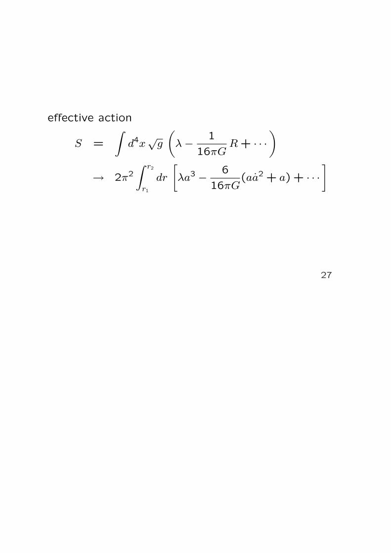
effective action

S =

∫d4x

√g

(λ− 1

16πGR + · · ·

)

→ 2π2

∫ r2

r1

dr

[λa3 − 6

16πG(aa2 + a) + · · ·

]

27

solutions of δS = 0

Gλ > 0 : a = r0 sinr

r0, R =

12

r20

= 32πGλ, S4

Gλ < 0 : a = r0 sinhr

r0, R =

−12

r20

= −32π|Gλ|, H4

try fitting∗ S4 (‘de Sitter’) in elongated phase,H4 (‘anti-de Sitter’) in crumpled phase

∗De Bakker, JS, NPB439(1995)239; S4 fits looked reasonable at

κ ≈ κc2, for 6 . r . rmax , H4 not done at the time.

28

crumpled phase

fit r0 sinh[(r − s0)/r0] to a(r)

e.g. in region where R < 0 (3 . r . 11)

or R < 0 after minimum of R (6 . r . 11)

elongated phase

fit r0 sin[(r − s0)/r0] to a(r) in region 4 ≤ r ≤ 11

29

0 5 10 15 20r

10

20

30

40

50aHrL

hyperbolic-sine fit to a(r) data at R < 0 (r = 3, . . . ,13), κ2 = 1.266,

r0 = 9.7, s0 = −2.2, crumpled phase

30

0 10 20 30 40 50r

5000

10 000

15 000

20 000

25 000

30 000aHrL^3

the fit to a(r)3

31

50 100 150 200 250 300r

100

200

300

400

500

N'Hr L

N ′(r) for κ2 = 1.3, N4 = 64000, elongated phase

32

4 6 8 10r

20

40

60

80

100

N'Hr L

close-up

33

0 2 4 6 8 10 12 14r

2

4

6

8

10

12aHrL

scale factor a(r)

34

10 20 30 40 50r

0.05

0.10

0.15

0.20RHrL

curvature R(r)

35

5 10 15 20r

6

8

10

12

aHrL

sine fit to a(r) data at r = 4,5, . . . ,11, r0 = 11.0, s0 = −3.0

36

20 40 60 80r

1000

2000

3000

4000

5000

aHrL^3

the fit to a(r)3

37

Test fields and particles

- do not ’back react’ on geometry

Scalar field

S = Sg + Sφ

Sg =1

16πG0

∫d4x

√g (2Λ0 −R)

Sφ =

∫d4x

√g

(1

2gµν∂µφ∂νφ +

1

2m2

0φ2

)

Z =

∫Dg Dφ e−S

〈O〉 =1

Z

∫Dg Dφ e−S O

38

interested in ⟨O(x)O′(y)|d(x,y)=r

⟩

e.g. O(x) = R(x), φ(x), φ(x)2, . . .

d(x, y) geodesic distance depends on g

implement as⟨∫

d4x√

g O(x)O′(y) δ[d(x, y)− r]∫d4x

√g δ[d(x, y)− r]

⟩

or (better)⟨∫

d4x√

g O(x)O′(y) δ[d(x, y)− r]⟩

⟨∫d4x

√g δ[d(x, y)− r]

⟩

- independent of y- non-local observables

39

φ test field: quenched approximation

Z =

∫Dg e−Sg [det(−¤ + m2

0)]−1/2

→Zg =

∫Dg e−Sg

Laplace-Beltrami operator ¤e.g. two-point function

G(r) =⟨φ(x)φ(y)|d(x,y)=r

⟩ → ⟨G(x, y)|d(x,y)=r

⟩g

=1

Zg

∫Dg e−Sg G(x, y)|d(x,y)=r

G(x, y) =[(−¤ + m2

0)−1

]x,y

40

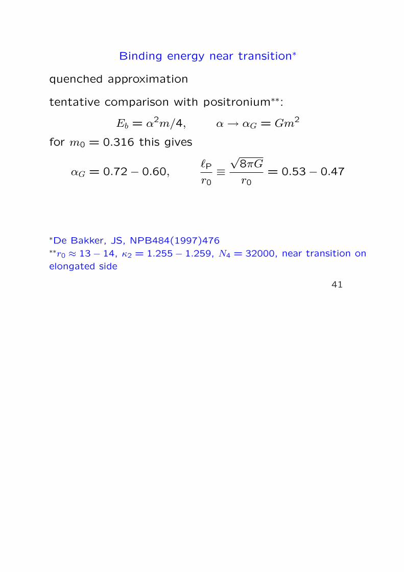
Binding energy near transition∗

quenched approximation

tentative comparison with positronium∗∗:

Eb = α2m/4, α → αG = Gm2

for m0 = 0.316 this gives

αG = 0.72− 0.60,`P

r0≡√

8πG

r0= 0.53− 0.47

∗De Bakker, JS, NPB484(1997)476∗∗r0 ≈ 13− 14, κ2 = 1.255− 1.259, N4 = 32000, near transition on

elongated side

41

Test in crumpled phase

massless minimally coupled scalar acquires effective masson space with constant negative curvature

a(r) = r0 sinh(r/r0), R = −12/r20

¤G(r) =

(d

dr+

3

r0coth

r

r0

)d

drG(r) = 0, r > 0

G(r) → 1

4πr2r → 0

→ 0 r →∞results in

G(r) =1

3πr20

e−3r/r0 +O(e−5r/r0), r →∞

43

effective mass

m =3

r0=

√−3

4R

compute G(r) in crumpled phase:

fit

G(r) = ce−mr + c′

44

0

0.2

0.4

0.6

0.8

1

1.2

1.4

0 10 20 30

1.2401.2451.2501.252

exponential fits to G(r), for N4 = 32000 and κ2 = 1.240, . . . , 1.252

45

0.04

0.06

0.08

0.1

0.12

0.14

0.16

0.18

0.2

1.24 1.25 1.26 1.27

m

κ2

3200064000

‘measured’ masses vs κ2 for N4 = 32000, 64000

46

-0.25

-0.2

-0.15

-0.1

-0.05

0

0.05

0.1

0.15

0.2

1.2 1.21 1.22 1.23 1.24 1.25 1.26 1.27 1.28 1.29 1.3

RV

κ2

3200064000

‘measured’ RV

47

good fits in 6 ≤ r ≤ 20!

m correlated with√

RV

expect m → 0 when curvature → 0(no additive mass renormalization)

consider power fit∗ to minimum of RW curvature

m = c(√−3Rmin/4)b

∗In binding-energy computation, mass renormalization can also be

fitted by power behavior, m2 ≈ 1.5(m20)

0.65

48

æ

æ

æ

æ

0.37 0.38 0.39 0.40-3 R 4

0.11

0.12

0.13

0.14

0.15

m

fit of c(√−3Rmin/4)b to induced-mass data, b = 3.7,

c = 4.35, N4 = 64000

49

Scaling

try scaling∗

ρ(x; τ) =rm

N4N ′(r;κ2, N4), x =

r

rm

N ′(r) is maximal at r = rm

τ = shape label, e.g. τ = ρ|x=1 or τ = κ2 at standard N4

∗De Bakker, JS, NPB439(1995)239

50

0 20 40 60 80 100r

500

1000

1500

2000

2500

N'Hr L

N ′(r) for κ2, N4 = 1.17,8000 (blue), 1.21,16000 (red),

1.240,32000 (brown) and 1.266,64000 (green)

51

0 1 2 3 4x

0.2

0.4

0.6

0.8

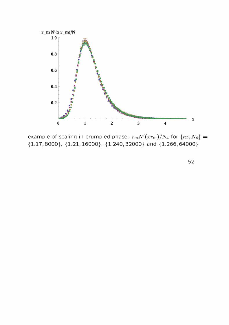
1.0r_m N'Hx r_mLN

example of scaling in crumpled phase: rmN ′(xrm)/N4 for κ2, N4 =

1.17,8000, 1.21,16000, 1.240,32000 and 1.266,64000

52

scaling dimension∗ ds: rm(κ2, N4) ∝ N1/ds

4

for pairs κ2, N4 belonging to the same scaling sequence(same τ)∗∗

ds ≈ 5.6

similar for rm → rav =∑

r rN ′(r)/N4

∗Sometimes identified with Hausdorff dimension, Ambjørn, Jurkiewicz,

NPB451(1995)643∗∗Neglecting κ2 dependence of rm or rav suggests ds →∞, Catterall,

Kogut, Renken, PLB328(1994)277; A &J.

53

scaling is approximate: deviations in small x region

rm not ∝ r0: r0 decreases as rm increases

54

Conclusion

- DT gives approximate continuum results at finitelattice spacing,

√G = O(`),

√Λ = O(`−1)

- scaling is large-scale phenomenon, does not imply`/√

G → 0, property of ground state

- crumpled phase: negative curvature

H4 is infinite, finite volume → ‘singular structure’?

55

- elongated phase: positive curvature

thick branched polymers

condensation of black holes? monsters?

- crucially important to resume study of ground statesand Q2 in EDT with matter, NV ≥ 1

56

-20

2

0

10

20

-2

0

2

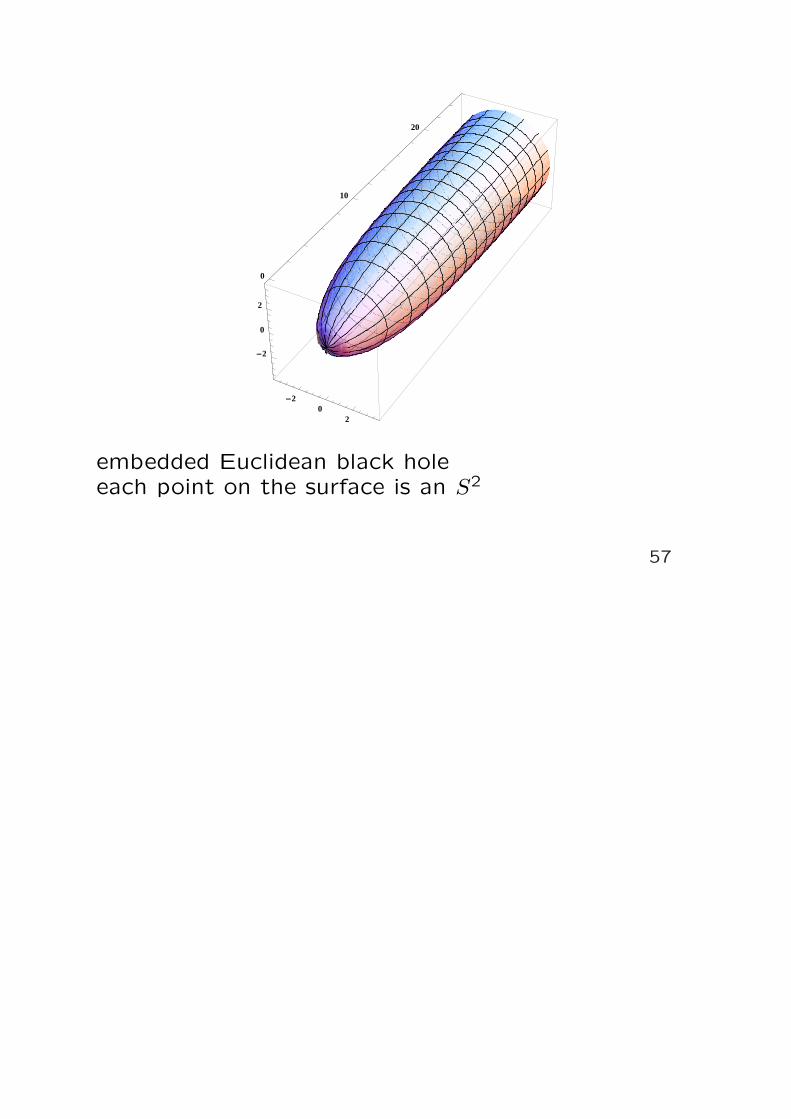
embedded Euclidean black holeeach point on the surface is an S2

57