groundwater flow drawdown

8/4/2019 Groundwater Flow Drawdown

http://slidepdf.com/reader/full/groundwater-flow-drawdown 1/10

Geol 121 Hydrology

Prof. J Bret Bennington Hydrology

Groundwater Flow in Aquifers / Drawdown in a Pumping Well

Introduction

We are now heading into a series of lectures where we will learn how to quantitatively

estimate groundwater flow, particularly flow to wells. We will also be learning how touse wells to test the parameters of an aquifer. Together, information on flow and aquifer

parameters are what hydrologists use to describe groundwater flow so that it can be

exploited and managed, and so that movement of contaminants can be estimated and

understood.

The equations for describing flow under different aquifer conditions are difficult to

derive, and there derivation is beyond the abilities of most of the people who use them.

They may look daunting, but all one really has to do to use them is the following:

1. Find the equation that is appropriate the problem at hand based on the information that

is needed and the type of aquifer setting in evidence.

2. Determine what information is needed to plug into the equation. Gather that

information and make sure that it is all in comparable and appropriate units.

3. Plug and chug - something that we are all getting good at by now.

4. Look at your answer and try to decide if it makes sense. Does it seem to be about the

right size?

Transmissivity

Let’s begin by returning for another look at transmissivity. This is sometimes a usefulquantity for describing an aquifer.

Transmissivity is equal to the hydraulic conductivity of an aquifer times the thickness of

the aquifer.

T = Kb

Transmissivity has units of L2 / time.

If we know the transmissivity of an aquifer we can use it to estimate the total flowthrough an aquifer of a constant width.

Q = TW dhdl

Steady flow in a confined aquifer



Geol 121 Hydrology

Prof. J Bret Bennington For example, we can estimate Steady flow in a confined aquifer using this equation.

We need to assume is that flow is horizontal within the aquifer, there is no leakage

through the bounding aquicludes, the aquifer is a constant thickness, and the hydraulic

gradient is linear.

Steady flow in an unconfined aquifer

To estimate steady flow in an unconfined aquifer is more difficult. Transmissivity has

less meaning in this case because the thickness of the saturated part of the aquifer is

not constant.

If water is flowing horizontally in an unconfined aquifer, then the hydraulic heads must

be decreasing in the direction of flow, which means that the water table is downwardsloping in the direction of flow.

If the thickness of the aquifer decreases, but the same volume of water is flowing, thenthe hydraulic gradient must be increasing toward the discharge area.

Dupuit (1863) derived an equation (the Dupuit equation) for flow in this situation, given

a set of assumptions called Dupuit Assumptions.

(Note: This will be typical of our work from now on. For each particular aquifer

situation, the equation that describes flow in that situation will be named for its inventor,

and will have a list of assumptions that must be met or at least approximated so that theresults of the equation are meaningful.)

The Dupuit equation:

q '=2

1 K h1

2 − h2

2

L

Where q’ is the flow per unit width (q’ x W = Q flow through the aquifer)

Assumptions:

dh = slope of water table

Flow is horizontal for small dh

Equipotentials are vertical

Groundwater Flow to Pumping Wells

In many ways, wells are the business of a hydrologist. Wells drilled into aquifers areused to monitor the aquifer, extract water from the aquifer for human use, extract



Geol 121 Hydrology

Prof. J Bret Bennington contaminated water from an aquifer, lower the water table for construction projects and

land drainage, and sometimes to re-inject water back into an aquifer.

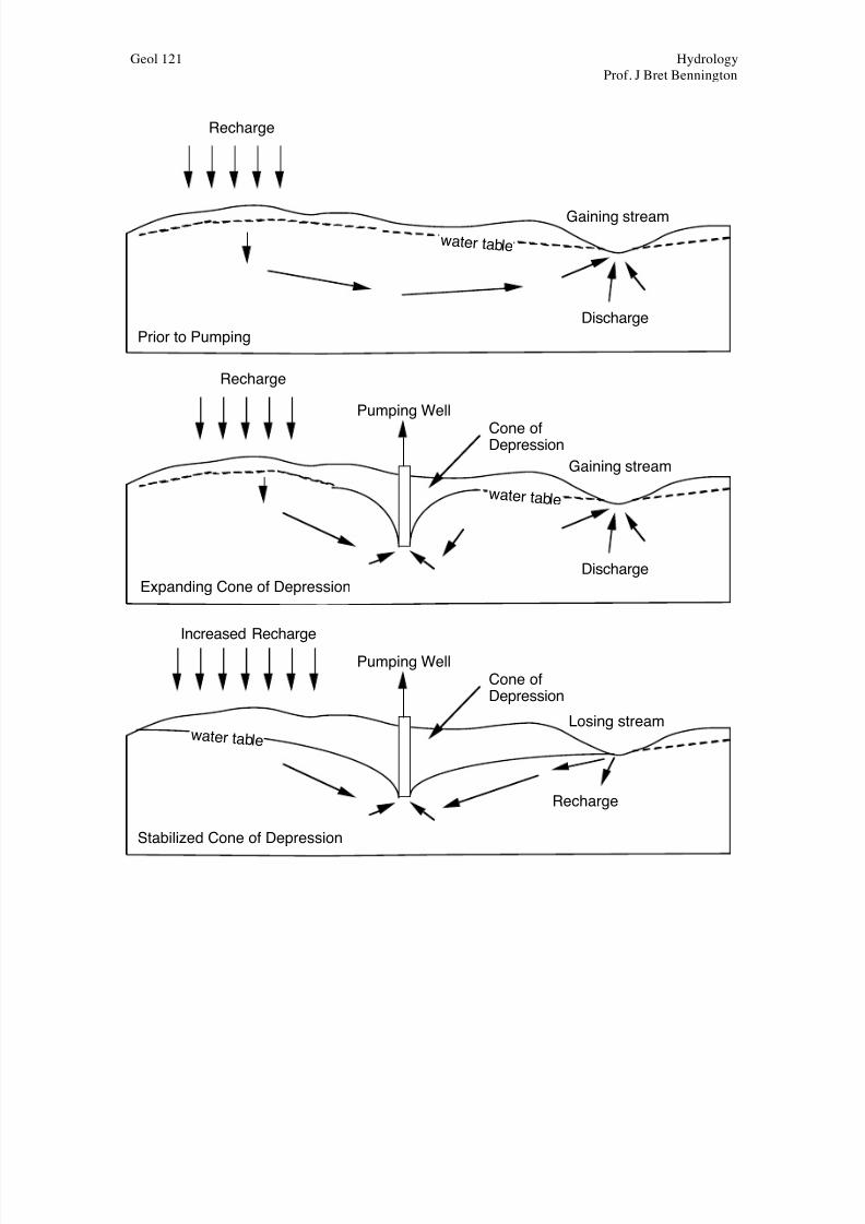
Pumping water from a well lowers the hydraulic head in a region around the site of

pumping. This causes a decline in the water table or potentiometric surface in the

vicinity of the well called a cone of depression (or pumping cone).

The decline in head values and / or water table level around a pumping well is called the

drawdown.

The size and shape of the cone of depression and the rate of drawdown are directly

related to the aquifer properties of storativity and transmissivity.

If we know the storativity and the transmissivity of an aquifer, then we can compute thesize and growth of the cone of depression for a given rate of pumping in a given aquifer.

Likewise, we can measure the rate of drawdown in a well and use this information toestimate the storativity and transmissivity of the aquifer. We will learn about various‘well tests’ that provide this information.

For the aquifer conditions that we will be dealing with, the following assumptions are

made:

1. The aquifer is bounded by a bottom confining layer.

2. All geologic formations are horizontal.3. The potentiometric surface is horizontal prior to pumping.

4. The potentiometric surface is stable prior to pumping.

5. The aquifer is homogeneous and isotropic.6. All flow is radial toward the well.7. Flow is horizontal.

8. Darcy’s law is valid.

9. The pumping well is fully screened through the entire thickness of the aquifer.

Before we proceed, let’s stop and think for a minute about where the water is coming

from that we are pumping out of an aquifer.

Storativity First, as we know from our studies of storativity, water that is in storage in an aquifer can

come from either changes in saturation of the aquifer, or changes in the pressure in anaquifer.

When an unconfined aquifer is pumped, the drawdown of the water table desaturates the

aquifer to liberate water that flows into the well.

When a confined aquifer is pumped, the drawdown of the potentiometric surface creates alowering of pressure in the cone of depression that liberates water to flow into the well.



Geol 121 Hydrology

Prof. J Bret Bennington As pumping continues, the cone of depression must grow larger and larger as more wateris removed from the aquifer.

Because the storativity of a confined aquifer is so much less than that of an unconfined

aquifer, the cone of depression from pumping a confined aquifer grows much morerapidly in extent than the cone of depression of an unconfined aquifer.

Recharge and discharge

If water is flowing through an aquifer, and if there is no change in storage over time, thenthe amount of recharge at one region of the aquifer must equal the amount of discharge at

another region.

If we begin pumping, we in effect add another source of discharge - one through the well.Now discharge will be greater than recharge, so storage must decrease - the cone of

depression expands.

The cone of depression will continue to expand until in reaches an area of discharge,recharge, or both.

If the cone of depression reaches an area of discharge, it will reverse the hydraulic

gradient and cause discharge to decrease or cease. For example, baseflow into a gainingstream might become baseflow from a losing stream if the cone of depression reaches the

stream.

The loss of discharge will slow the loss from storage due to pumping by decreasing the

overall discharge, resulting in a slowing of the expansion of the cone of depression. If

the decrease in discharge is great enough, recharge and discharge may balance and thecone of depression will stabilize.

If the cone of depression reaches an area of recharge, then, provided there is an excess of

water available for recharge (i.e. not all water available is infiltrating), the rate of

recharge will increase.

Recharge increases because the cone of depression brings with it a steeper hydraulic

gradient, allowing recharging water to move into the aquifer at a faster rate. Again, if the

increase in recharge is large enough to balance the loss due to discharge, then the cone of depression will stabilize.

Generally in the eastern United States there are many gaining streams that are relatively

closely spaced, with few areas with excess recharge. Therefore, wells tend to effectdischarge areas, and pumping often changes gaining streams into losing streams. If these

streams are polluted, this is a potential problem as the contaminated water can be drawn

into the aquifer.



Geol 121 Hydrology

Prof. J Bret Bennington

Discharge

Recharge

Discharge

Recharge

Pumping Well

Cone ofDepression

Increased Recharge

Recharge

Pumping WellCone ofDepression

Gaining stream

Gaining stream

Losing stream

Prior to Pumping

Expanding Cone of Depression

Stabilized Cone of Depression

w at er t able

w at er t able

w at er t able



Geol 121 Hydrology

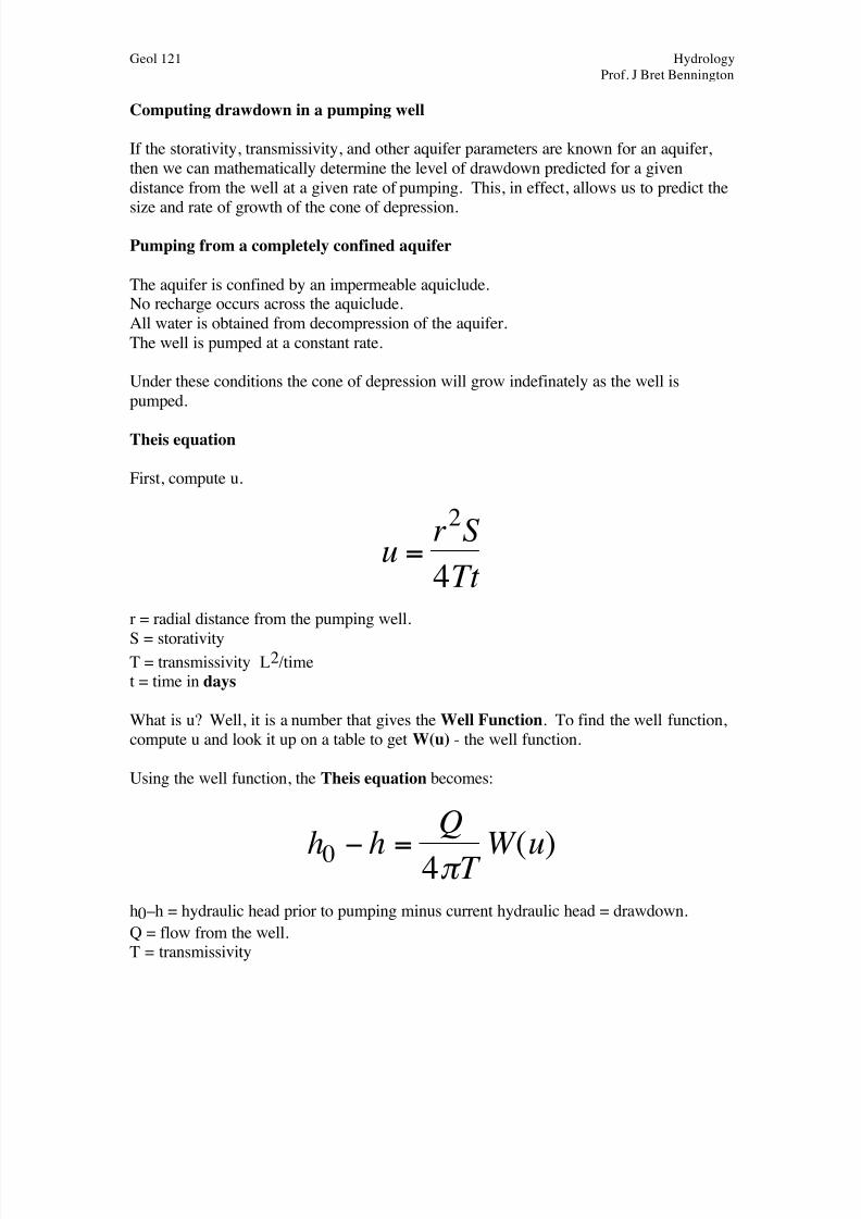
Prof. J Bret Bennington Computing drawdown in a pumping well

If the storativity, transmissivity, and other aquifer parameters are known for an aquifer,

then we can mathematically determine the level of drawdown predicted for a given

distance from the well at a given rate of pumping. This, in effect, allows us to predict the

size and rate of growth of the cone of depression.

Pumping from a completely confined aquifer

The aquifer is confined by an impermeable aquiclude.No recharge occurs across the aquiclude.

All water is obtained from decompression of the aquifer.

The well is pumped at a constant rate.

Under these conditions the cone of depression will grow indefinately as the well is

pumped.

Theis equation

First, compute u.

u =r2S

4Tt

r = radial distance from the pumping well.

S = storativityT = transmissivity L2/timet = time in days

What is u? Well, it is a number that gives the Well Function. To find the well function,

compute u and look it up on a table to get W(u) - the well function.

Using the well function, the Theis equation becomes:

h0−

h=

Q

4π T W (u)

h0 –h = hydraulic head prior to pumping minus current hydraulic head = drawdown.

Q = flow from the well.T = transmissivity



Geol 121 Hydrology

Prof. J Bret Bennington As you can see, this equation will give you the drawdown of the potentiometric surface

that will be seen some distance away from a well, so many days after a given rate of pumping begins.

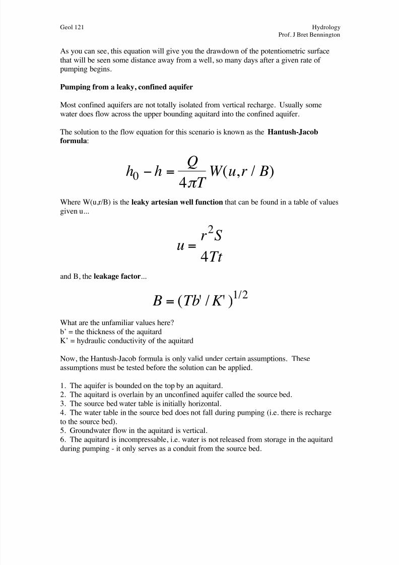
Pumping from a leaky, confined aquifer

Most confined aquifers are not totally isolated from vertical recharge. Usually some

water does flow across the upper bounding aquitard into the confined aquifer.

The solution to the flow equation for this scenario is known as the Hantush-Jacob

formula:

h0 − h =Q

4π T W (u,r / B)

Where W(u,r/B) is the leaky artesian well function that can be found in a table of values

given u...

u =r2S

4Tt

and B, the leakage factor...

B = (Tb' /K ' )1/2

What are the unfamiliar values here?

b’ = the thickness of the aquitard

K’ = hydraulic conductivity of the aquitard

Now, the Hantush-Jacob formula is only valid under certain assumptions. These

assumptions must be tested before the solution can be applied.

1. The aquifer is bounded on the top by an aquitard.

2. The aquitard is overlain by an unconfined aquifer called the source bed.3. The source bed water table is initially horizontal.

4. The water table in the source bed does not fall during pumping (i.e. there is recharge

to the source bed).5. Groundwater flow in the aquitard is vertical.

6. The aquitard is incompressable, i.e. water is not released from storage in the aquitard

during pumping - it only serves as a conduit from the source bed.



Geol 121 Hydrology

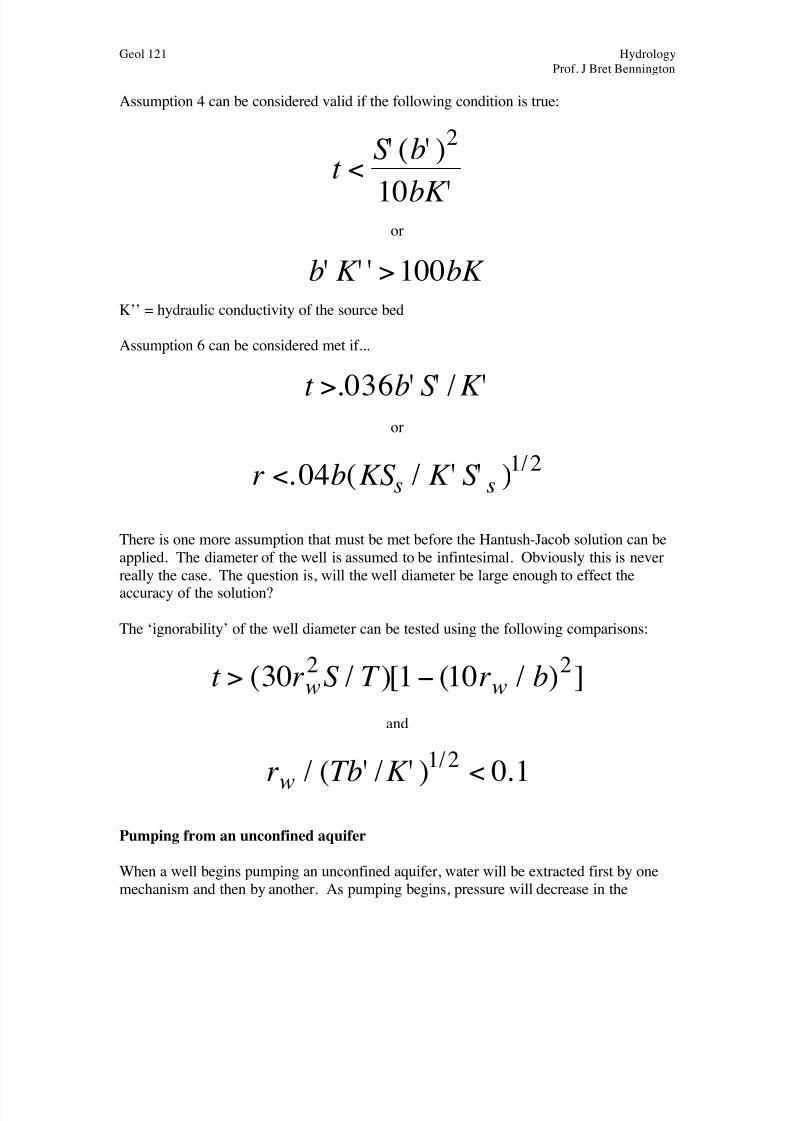
Prof. J Bret Bennington Assumption 4 can be considered valid if the following condition is true:

t <S ' (b' )

2

10bK '

or

b' K ' ' >100bK

K’’ = hydraulic conductivity of the source bed

Assumption 6 can be considered met if...

t >.036b' S ' /K '

or

r <.04b(KS s / K ' S ' s )1/2

There is one more assumption that must be met before the Hantush-Jacob solution can be

applied. The diameter of the well is assumed to be infintesimal. Obviously this is never

really the case. The question is, will the well diameter be large enough to effect the

accuracy of the solution?

The ‘ignorability’ of the well diameter can be tested using the following comparisons:

t > (30rw2S / T )[1− (10rw / b)

2]

and

rw / (

Tb' /K

' )

1/ 2<

0.1

Pumping from an unconfined aquifer

When a well begins pumping an unconfined aquifer, water will be extracted first by one

mechanism and then by another. As pumping begins, pressure will decrease in the



Geol 121 Hydrology

Prof. J Bret Bennington aquifer in the vicinity of the well. This will cause the unconfined aquifer to behave, at

first, like a confined aquifer. Water will be released from specific storage.

However, not long after pumping begins, the water table begins to draw down in the

vicinity of the well, and now the aquifer is being drained and storativity is equal not to

specific storage, but to specific yield.

The solution to flow in an unconfined aquifer being pumped has been worked out by

Neuman. Neuman’s solution is based on the following assumptions:

1. Aquifer is unconfined.

2. The vadose zone has no influence on drawdown.

3. Drawdown is very small relative to the thickness of the aquifer.

4. Specific yield is 10 times greater than specific storage.

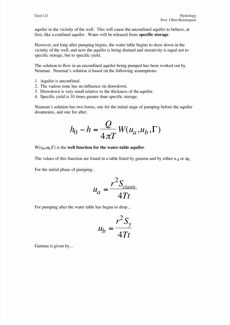
Neuman’s solution has two forms, one for the initial stage of pumping before the aquifer

desaturates, and one for after.

h0 − h =Q

4π T W (ua ,ub ,Γ)

W(ua,ub,Γ) is the well function for the water-table aquifer.

The values of this function are found in a table listed by gamma and by either ua or ub.

For the initial phase of pumping..

ua =r2S elastic

4Tt

For pumping after the water table has begun to drop...

ub =r2S y

4Tt

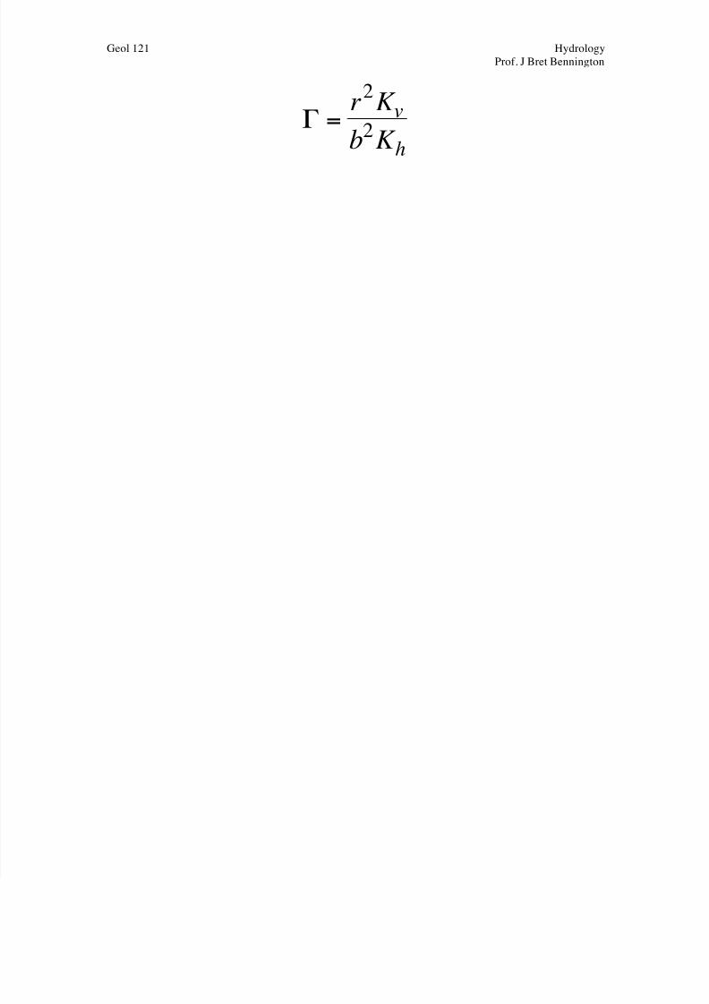
Gamma is given by...



Geol 121 Hydrology

Prof. J Bret Bennington

Γ =

r2K v

b2K h

groundwater flow drawdown

Documents