Case Study

Groundwater Flow Modeling of a Hard RockAquifer: Case Study

V. Varalakshmi1; B. Venkateswara Rao2; L. SuriNaidu3; and M. Tejaswini4

Abstract: The present study area is primarily underlain by granites, basalts, and a little bit of laterites. Groundwater occurs under unconfinedto semiconfined conditions, in weathered and fractured formations, respectively. A three-dimensional groundwater flow model for theOsmansagar and Himayathsagar catchments—a semiarid hard rock area in India with two conceptual layers—is developed under transientconditions using visual MODFLOW software for the period 2005 to 2009. The 15–20 m top layer is a weathered zone, followed by second20–25 m-layer fractured zone based on hydrogeophysical studies and borehole lithologs. The groundwater recharge estimation is achievedwith the help of geographical information system (GIS) and the water table fluctuation method that is well fitted into the flow model with anaverage recharge value of 21% of the average annual rainfall. The results derived from modeling indicate that the average input to the aquifersystem is 321.96 million cubic meters (mcm), and the output is 322.14 mcm. If the same withdrawal is continued up until the year 2020, thewater level is believed to decline more than 45 m over the entire study area. To avoid this critical stage, the present draft should be decreasedby nearly 40%. DOI: 10.1061/(ASCE)HE.1943-5584.0000627. © 2014 American Society of Civil Engineers.

Author keywords: Groundwater flow model; Transient state; Hard rock aquifer; Groundwater recharge and draft.

Introduction

A hard rock aquifer occupies the first few tens of meters from thetop (Detay et al. 1989; Taylor and Howard 2000) that is subjected tothe weathering process (Wyns et al. 2004). Groundwater occurs inthe weathered and fractured layers under unconfined to semicon-fined conditions, which have specific hydrodynamic propertiesfrom the top to the bottom. Quantification of groundwater resour-ces and understanding of hydrogeologic processes are a basic pre-requisite for efficient and sustainable management of groundwaterresource development and management (Sophocleous 1991; Vander Gun and Lipponen 2010). This is particularly vital for India,where 80% of the Indian peninsula is covered with hard rocks,coupled with a widely prevalent semiarid climate (Pathak 1984).Because of the increasing demand of water for agriculture, indus-tries, and ever-growing population requirements, the abstraction ofgroundwater has increased in the last few decades. The heavy de-mand for groundwater sometimes leads to excessive groundwaterwithdrawals, which is often reflected in a serious imbalance be-tween groundwater draft and recharge at a later stage. Aquifer mod-eling is an established tool to study the behavior of the groundwaterregime under spatio-temporal variation of input and output stresses.The findings in turn help to evolve and select optimal groundwater

exploitation and management policies. However, modeling of anaquifer in a hard rock region is quite a difficult task because of highheterogeneity (Singhal and Gupta 1999; Bridget et al. 2003; Nicoand David 2007). This inherently renders the discretization of themedium and interpolation of the hydrogeological parameters to berelatively difficult and at times unrealistic. In spite of these diffi-culties, many researchers have successfully used numerical modelsin estimating the regional groundwater budget in hard rocks, moun-tainous regions, and in karst aquifer groundwater systems (Raniand Chen 2010; Majumdar et al. 2009; Bridget et al. 2003;Surinaidu et al. 2013a, b). Therefore, in the present study, varioushydrogeological factors are appropriately considered to representthe hard rock aquifer system to a satisfactory degree on a regionalscale using a USGS finite difference numerical model.

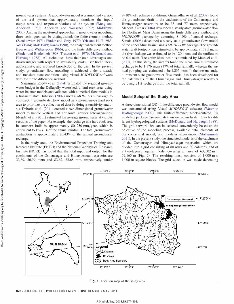
The area chosen for aquifer modeling is the catchment areas ofthe Osmansagar and Himayatsagar reservoirs. The area is across theMusi and Musa rivers and supplies the drinking water for the city ofHyderabad. It is situated between 17°10′–17°50′N and 78°10′ to 78°50′ E, covering an area of 2,030 km2 (Fig. 1). The drainage patternis dendritic to subdendritic and trelliss (Gurunadharao et al. 2008).The terrain is flat to gently undulating, except for a few hillocks andvalleys. The region is primarily underlain by a peninsular gneissiccomplex that includes a variety of granites, magmatites of variousphases, and enclaves of older metamorphic rocks belonging to theArchean age. These are intruded by various acidic (pegmatite, ap-tite, quartz veins/reefs) and basic intrusives of dolerite and gabbros.Major dykes of dolerite composition cut across the country rocks indifferent directions. The predominant soils in the basin are sandyloam, clay loam, black cotton soils, and rocky soils. The riverbedis mostly deposited with sandy soils. Groundwater occurs underunconfined to semiconfined conditions in weathered and fracturedformations, respectively.

Literature Review

Groundwater modeling is increasingly recognized as a powerfulquantitative tool available to hydrogeologists for evaluating

1Lecturer, Centre for Water Resources, Jawaharlal Nehru TechnologicalUniv., Hyderabad 500085, India.

2Professor of Water Resources and Coordinator of CEA & WMT,JNTUH, Hyderabad 500085, India (corresponding author). E-mail:cwr_jntu@yahoo.com

3Special Project Scientist, International Water Management Institute,Hyderabad, India.

4Postgraduate Student, Centre for Water Resources, Jawaharlal NehruTechnological Univ., Hyderabad 500085, India.

Note. This manuscript was submitted on April 8, 2011; approved onMarch 23, 2012; published online on March 27, 2012. Discussion periodopen until October 1, 2014; separate discussions must be submitted for in-dividual papers. This paper is part of the Journal of Hydrologic Engineer-ing, Vol. 19, No. 5, May 1, 2014. © ASCE, ISSN 1084-0699/2014/5-877-886/$25.00.

JOURNAL OF HYDROLOGIC ENGINEERING © ASCE / MAY 2014 / 877

J. Hydrol. Eng. 2014.19:877-886.

Dow

nloa

ded

from

asc

elib

rary

.org

by

Jaw

ahar

lal N

ehru

Tec

hnol

ogic

al U

nive

rsity

on

11/0

2/14

. Cop

yrig

ht A

SCE

. For

per

sona

l use

onl

y; a

ll ri

ghts

res

erve

d.

groundwater systems. A groundwater model is a simplified versionof the real system that approximately simulates the input/output stress and response relations of the system (Wang andAnderson 1982; Anderson and Woessner 1992; Middlemis2000). Among the most-used approaches in groundwater modeling,three techniques can be distinguished: the finite-element method(Zienkiewicz 1971; Pinder and Gray 1977; Yeh and Huff 1983;Voss 1984; Istok 1989; Kazda 1990), the analytical element method(Freeze and Witherspoon 1966), and the finite difference method(Pinder and Bredehoeft 1968; Trescott et al. 1976; McDonald andHarbaugh 1988). All techniques have their own advantages anddisadvantages with respect to availability, costs, user friendliness,applicability, and required knowledge of the user. In the presentstudy, groundwater flow modeling is achieved under a steadyand transient state condition using visual MODFLOW softwarewith the finite difference method.

Narasimha Reddy et al. (1994) estimated the regional ground-water budget in the Dullapally watershed, a hard rock area, usingwater-balance models and validated with numerical flow models ina transient state. Johnson (2007) used a MODFLOW package toconstruct a groundwater flow model in a mountainous hard rockarea to prioritize the collection of data by doing a sensitivity analy-sis. Dehotin et al. (2011) created a two-dimensional groundwatermodel to handle vertical and horizontal aquifer heterogeneities.Mondal et al. (2011) estimated the average groundwater at varioussections of the paper. For example, the recharge in a hard rock areain southern India is approximately 80–250 mm=year, which isequivalent to 12–37% of the annual rainfall. The total groundwaterabstraction is approximately 80.43% of the annual groundwaterrecharge.

In the study area, the Environmental Protection Training andResearch Institute (EPTRI) and the National Geophysical ResearchInstitute (NGRI) has found that the total input and output for thecatchments of the Osmansagar and Himayatsagar reservoirs are33.69, 36.99 mcm and 83.62, 82.68 mm, respectively, under

8–10% of recharge conditions. Gurunadharao et al. (2008) foundthe groundwater draft in the catchments of the Osmansagar andHimayatsagar reservoirs to be 35 and 77 mcm, respectively.Mahesh Kumar (2004) developed a steady-state groundwater flowfor Northeast Musi Basin using the finite difference method andMODFLOW package by assuming 8–10% of annual recharge.Sarada (2006) developed a steady-state groundwater flow modelof the upper Musi basin using aMODFLOW package. The ground-water draft (output) was estimated to be approximately 177.5 mcm;the river leakage was estimated to be 120 mcm; and the outflow tobe 0.4 mcm. The entire Musi basin is simulated by Massuel et al.(2007). In this study, the authors found the mean annual simulatedrecharge to be 1,176 mcm (17% of total rainfall), whereas the an-nual pumping was estimated to be 1,235 mcm. In the present study,a transient-state groundwater flow model has been developed forthe catchments of the Osmansagar and Himayatsagar reservoirsby using 21% recharge from the total rainfall.

Model Setup of the Study Area

A three-dimensional (3D) finite-difference groundwater flow modelwas constructed using Visual MODLFOW software (WaterlooHydrogeologic 2002). This finite-difference, block-centered, 3Dmodeling package can simulate transient groundwater flows for dif-ferent hydrogeological systems (McDonald and Harbaugh 1988).The grid network size can be selected conveniently based on theobjective of the modeling process, available data, elements ofthe conceptual model, and modeler experiences (Mohammadi2011). In the present study, the simulated model is of the catchmentof the Osmansagar and Himayathsagar reservoirs, which aredivided into a grid consisting of 80 rows and 80 columns, and ofa two-layered aquifer model covering an area of 63; 502 m ×57,165 m (Fig. 2). The resulting mesh consists of 1,000 m ×1,000 m square blocks. The grid selection was made depending

Fig. 1. Location map of the study area

878 / JOURNAL OF HYDROLOGIC ENGINEERING © ASCE / MAY 2014

J. Hydrol. Eng. 2014.19:877-886.

Dow

nloa

ded

from

asc

elib

rary

.org

by

Jaw

ahar

lal N

ehru

Tec

hnol

ogic

al U

nive

rsity

on

11/0

2/14

. Cop

yrig

ht A

SCE

. For

per

sona

l use

onl

y; a

ll ri

ghts

res

erve

d.

on the data availability. The available data were adequate to re-present the fluxes across the watersheds. Based on the analysisof 1D and 2D resistivity data in the study area, the two-layer modelis considered for the modeling because these two layers are the onlysaturated water columns. The first layer consists mostly of a 15–20 m weathered zone and is underlain by a 20–25 m-thick fracturedzone. The simulated vertical section has a total thickness of approx-imately 35–45 m. The top layer represents the weathered portion inthe system, which is typically designated as an unconfined layer,and the second layer represents the fractured zone and is assumedto represent semiconfined to unconfined conditions with variable T

and S (Figs. 3 and 4). Both layers are hydraulically connected(Briz-Kishore and Bhimasankaram 1982)

The basic assumptions made regarding the aquifer modeling arethat the Musi and Musa rivers are ephemeral rivers and may be-come affluent and influent depending on the river flows and sur-rounding groundwater conditions; thus, they are simulated by theMODFLOW river package. No flow occurs across catchment boun-daries, as these boundaries coincide approximately with ground-water divides and continuous leakage will occur to the fracturedzone from the overlying weathered zone. As the aquifer is a closedone with a streamlet, some outflow may take place. Seepage from

Fig. 2. Model grid domain

Fig. 3. Horizontal cross-section of aquifer layers (row 44)

Fig. 4. Vertical cross-section of aquifer layers (column 44) Fig. 5. Boundary conditions in the study area

JOURNAL OF HYDROLOGIC ENGINEERING © ASCE / MAY 2014 / 879

J. Hydrol. Eng. 2014.19:877-886.

Dow

nloa

ded

from

asc

elib

rary

.org

by

Jaw

ahar

lal N

ehru

Tec

hnol

ogic

al U

nive

rsity

on

11/0

2/14

. Cop

yrig

ht A

SCE

. For

per

sona

l use

onl

y; a

ll ri

ghts

res

erve

d.

the surface water bodies and streams are additional input to thewatershed recharging system (Venkateswara Rao 2006). The delayin recharge to the aquifer is inappreciable, and the hydrogeologicalparameters do not change during the period for which the aquifer issimulated.

Boundary Conditions

The boundary conditions are a key component of the conceptuali-zation of a groundwater flow system (Franke et al. 1987; Reilly2001). The MODFLOW river package is used to incorporate sur-face water boundary conditions into the groundwater flow model(Fig. 5). Lakes, streams, and drains contribute to the groundwater

system based on the gradient between the surface water body andgroundwater regime. The surface water and aquifer interactionwas simulated by assigning water levels and streambed elevationsof the streams in the study area. The outflow towards the MusiRiver, at the west in the study area, was simulated as a constanthead of 540 and 530 m, respectively, for the Osmansagar andHimayatsagar reservoirs in the model. The river stage elevationof the water body is the elevation of the water surface of the surfacewater body. The river bottom elevation is the elevation of thestream. Conductance is a numerical parameter that representsthe resistance to flow between the surface water body and thegroundwater.

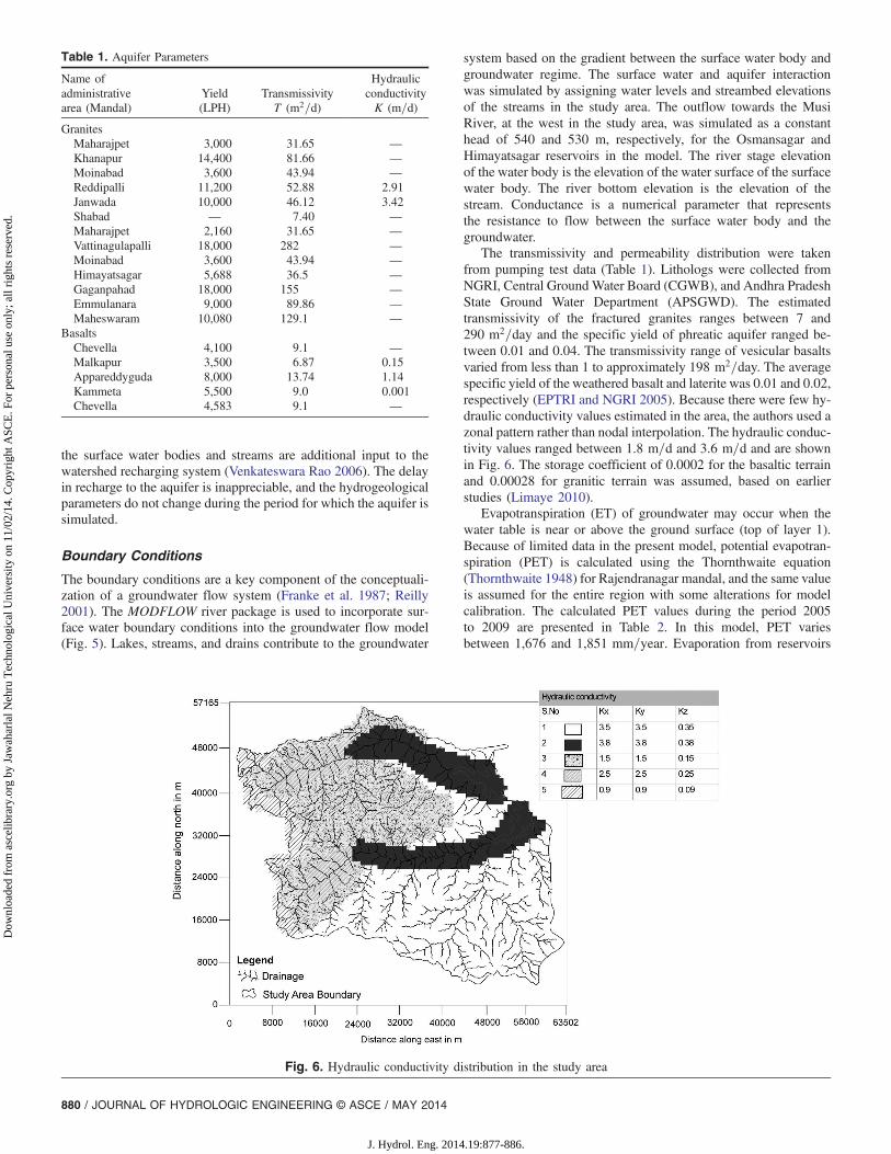
The transmissivity and permeability distribution were takenfrom pumping test data (Table 1). Lithologs were collected fromNGRI, Central GroundWater Board (CGWB), and Andhra PradeshState Ground Water Department (APSGWD). The estimatedtransmissivity of the fractured granites ranges between 7 and290 m2=day and the specific yield of phreatic aquifer ranged be-tween 0.01 and 0.04. The transmissivity range of vesicular basaltsvaried from less than 1 to approximately 198 m2=day. The averagespecific yield of the weathered basalt and laterite was 0.01 and 0.02,respectively (EPTRI and NGRI 2005). Because there were few hy-draulic conductivity values estimated in the area, the authors used azonal pattern rather than nodal interpolation. The hydraulic conduc-tivity values ranged between 1.8 m=d and 3.6 m=d and are shownin Fig. 6. The storage coefficient of 0.0002 for the basaltic terrainand 0.00028 for granitic terrain was assumed, based on earlierstudies (Limaye 2010).

Evapotranspiration (ET) of groundwater may occur when thewater table is near or above the ground surface (top of layer 1).Because of limited data in the present model, potential evapotran-spiration (PET) is calculated using the Thornthwaite equation(Thornthwaite 1948) for Rajendranagar mandal, and the same valueis assumed for the entire region with some alterations for modelcalibration. The calculated PET values during the period 2005to 2009 are presented in Table 2. In this model, PET variesbetween 1,676 and 1,851 mm=year. Evaporation from reservoirs

Table 1. Aquifer Parameters

Name ofadministrativearea (Mandal)

Yield(LPH)

TransmissivityT (m2=d)

HydraulicconductivityK (m=d)

GranitesMaharajpet 3,000 31.65 —Khanapur 14,400 81.66 —Moinabad 3,600 43.94 —Reddipalli 11,200 52.88 2.91Janwada 10,000 46.12 3.42Shabad — 7.40 —Maharajpet 2,160 31.65 —Vattinagulapalli 18,000 282 —Moinabad 3,600 43.94 —Himayatsagar 5,688 36.5 —Gaganpahad 18,000 155 —Emmulanara 9,000 89.86 —Maheswaram 10,080 129.1 —

BasaltsChevella 4,100 9.1 —Malkapur 3,500 6.87 0.15Appareddyguda 8,000 13.74 1.14Kammeta 5,500 9.0 0.001Chevella 4,583 9.1 —

Fig. 6. Hydraulic conductivity distribution in the study area

880 / JOURNAL OF HYDROLOGIC ENGINEERING © ASCE / MAY 2014

J. Hydrol. Eng. 2014.19:877-886.

Dow

nloa

ded

from

asc

elib

rary

.org

by

Jaw

ahar

lal N

ehru

Tec

hnol

ogic

al U

nive

rsity

on

11/0

2/14

. Cop

yrig

ht A

SCE

. For

per

sona

l use

onl

y; a

ll ri

ghts

res

erve

d.

is approximately 2,311 mm=year, which is adopted from the Hy-derabad Municipal Water Supply and Sewage Board (HMWS& SB).

Input and Output Stresses

Recharge to the groundwater regime resulting from monsoon rain-fall, seepage from surface water bodies, and irrigation return seep-age from fields contribute as inputs to the aquifer system. Theoutflow occurs primarily through groundwater withdrawal fromwells for irrigation and evapotranspiration, and acts as output.

Estimation of Groundwater Recharge by Water TableFluctuation Method

In the present study, premonsoon and postmonsoon groundwaterlevels are observed in the year 2005, 2006, 2008, and 2009 at

26 locations covering the catchment areas of the Osmansagarand Himayatsagar reservoirs. These levels are reduced to meansea level and the difference between premonsoon and postmonsoonlevels are contoured using Arc GIS software. The water-levelfluctuation contours for the year 2005 are shown in Fig. 7. Areasbetween successive contours of the groundwater-level fluctuations(Fig. 7) are estimated by using the Arc GIS software and the spe-cific yield (Sy) values of different formations are adopted from therecommended values of the Ground Water Estimation Committee[Ground Water Estimation Committee (GEC) 1997]. Based onlocal geology, the recharge is estimated by using the formula

Recharge ¼ Geographical area ×Water table fluctuation

× Specific yield ð1Þ

The average annual rainfall during the years 2005 to 2009 in thestudy area and the estimated recharge resulting from rainfall isshown in the Table 3. The percentage of rainfall converted intogroundwater recharge is also shown in this table. On average,nearly 21% of rainfall joins the groundwater by direct infiltrationof rainfall and by recharge through various water-conservationstructures such as tanks, reservoirs, and check dams. These ob-servations are almost tallying with the earlier studies carried outby International Crops Research Institute for the Semi-Arid Tropics

Table 2. Variations in Monthly PET during 2005–2009

Months

Years (mm)

2005 2006 2007 2008 2009

January 70.83 51.54 58.34 74.0 54.2February 76.52 59.96 70.66 81.1 63.9March 144.03 136.52 159.79 151.3 141.0April 220.63 215.88 222.99 228.2 221.8May 311.52 275.38 316.40 320.8 282.5June 281.27 209.59 209.78 290.0 214.7July 198.12 202.15 131.55 202.6 206.9August 143.08 141.66 153.00 146.7 146.9September 124.85 136.39 128.90 128.5 141.6October 115.20 115.01 108.63 118.7 119.4November 53.95 78.67 57.71 57.2 82.8December 48.98 53.02 65.04 51.6 57.4Total 1,789.03 1,675.83 1,682.83 1,850.84 1,733.05

Fig. 7. Water table fluctuation contours during the year 2005

Table 3. Percent Rainfall Converted into Groundwater Recharge

YearRainfall(mm)

Rainfall(mcm)

Total amount ofrecharge (mcm)

Percent rainfall convertedinto groundwater

recharge

2005 955.45 1,952.43 416.10 21.312006 603.12 1,207.27 239.69 19.852008 898.39 1,892.16 441.80 23.072009 720.39 1,532.00 313.27 20.56Average 789.35 1,597.17 347.62 21.19

JOURNAL OF HYDROLOGIC ENGINEERING © ASCE / MAY 2014 / 881

J. Hydrol. Eng. 2014.19:877-886.

Dow

nloa

ded

from

asc

elib

rary

.org

by

Jaw

ahar

lal N

ehru

Tec

hnol

ogic

al U

nive

rsity

on

11/0

2/14

. Cop

yrig

ht A

SCE

. For

per

sona

l use

onl

y; a

ll ri

ghts

res

erve

d.

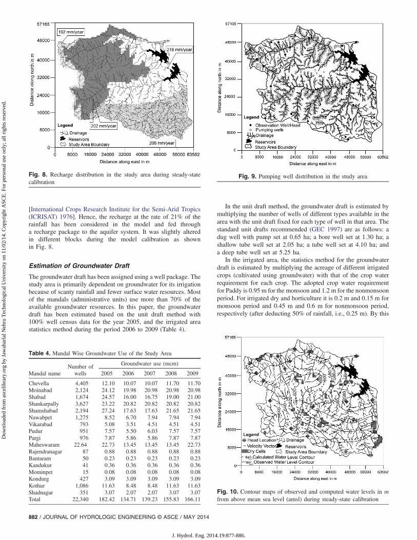
[International Crops Research Institute for the Semi-Arid Tropics(ICRISAT) 1976]. Hence, the recharge at the rate of 21% of therainfall has been considered in the model and fed througha recharge package to the aquifer system. It was slightly alteredin different blocks during the model calibration as shownin Fig. 8.

Estimation of Groundwater Draft

The groundwater draft has been assigned using a well package. Thestudy area is primarily dependent on groundwater for its irrigationbecause of scanty rainfall and fewer surface water resources. Mostof the mandals (administrative units) use more than 70% of theavailable groundwater resources. In this paper, the groundwaterdraft has been estimated based on the unit draft method with100% well census data for the year 2005, and the irrigated areastatistics method during the period 2006 to 2009 (Table 4).

In the unit draft method, the groundwater draft is estimated bymultiplying the number of wells of different types available in thearea with the unit draft fixed for each type of well in that area. Thestandard unit drafts recommended (GEC 1997) are as follows: adug well with pump set at 0.65 ha; a bore well set at 1.30 ha; ashallow tube well set at 2.05 ha; a tube well set at 4.10 ha; anda deep tube well set at 5.25 ha.

In the irrigated area, the statistics method for the groundwaterdraft is estimated by multiplying the acreage of different irrigatedcrops (cultivated using groundwater) with that of the crop waterrequirement for each crop. The adopted crop water requirementfor Paddy is 0.95 m for the monsoon and 1.2 m for the nonmonsoonperiod. For irrigated dry and horticulture it is 0.2 m and 0.15 m formonsoon period and 0.45 m and 0.6 m for nonmonsoon period,respectively (after deducting 50% of rainfall, i.e., 0.25 m). By this

Fig. 8. Recharge distribution in the study area during steady-statecalibration

Table 4. Mandal Wise Groundwater Use of the Study Area

Mandal nameNumber of

wells

Groundwater use (mcm)

2005 2006 2007 2008 2009

Chevella 4,405 12.10 10.07 10.07 11.70 11.70Moinabad 2,124 24.12 19.98 20.98 20.98 20.98Shabad 1,674 24.57 16.00 16.75 19.00 21.00Shankarpally 3,627 23.22 20.82 20.82 20.82 20.82Shamshabad 2,194 27.24 17.63 17.63 21.65 21.65Nawabpet 1,275 8.52 6.70 7.94 7.94 7.94Vikarabad 793 5.08 3.51 4.51 4.51 4.51Pudur 951 7.57 5.50 6.03 7.57 7.57Pargi 976 7.87 5.86 5.86 7.87 7.87Maheswaram 22.64 22.73 13.45 13.45 13.45 22.73Rajendranagar 87 0.88 0.88 0.88 0.88 0.88Bantaram 50 0.23 0.23 0.23 0.23 0.23Kandukur 41 0.36 0.36 0.36 0.36 0.36Mominpet 15 0.08 0.08 0.08 0.08 0.08Kondurg 427 3.09 3.09 3.09 3.09 3.09Kothur 1,086 11.63 8.48 8.48 11.63 11.63Shadnagar 351 3.07 2.07 2.07 3.07 3.07Total 22,340 182.42 134.71 139.23 155.83 166.11

Fig. 9. Pumping well distribution in the study area

Fig. 10. Contour maps of observed and computed water levels in mfrom above mean sea level (amsl) during steady-state calibration

882 / JOURNAL OF HYDROLOGIC ENGINEERING © ASCE / MAY 2014

J. Hydrol. Eng. 2014.19:877-886.

Dow

nloa

ded

from

asc

elib

rary

.org

by

Jaw

ahar

lal N

ehru

Tec

hnol

ogic

al U

nive

rsity

on

11/0

2/14

. Cop

yrig

ht A

SCE

. For

per

sona

l use

onl

y; a

ll ri

ghts

res

erve

d.

method, the total groundwater draft for irrigation was calculatedusing the following formula:

Total draft ¼ Area irrigated × Cropwater requirement ð2Þ

Table 4 shows that the groundwater draft is more in the mandalsof Moinabad, Maheswaram, Shabad, Shankarpally, Shamshabad,and Chevella. The groundwater withdrawal in the catchment areaswas simulated appropriately through well package with ground-water pumping rates varying between 100 and 500 m3=day pergrid, considering the urbanization, land use etc. (Fig. 9).

Calibration and Validation of the Model

A steady-state calibration is accomplished for the year 2005 post-monsoon. The general groundwater flow direction is from west toeast. The total input to the aquifer is 354.26535 mcm, and the totaloutput is 354.26955 mcm. This indicates that the deficiency ofrecharge of 0.0042 mcm is responsible for the decline of the watertable in the region. The computed and observed water levels duringsteady state are shown in Fig. 10. The calibrated steady-state modelconditions have been used as initial conditions for the transientmodel. The transient-state groundwater flow model was developedfor a five-year period from November 2005 to November 2009, andthe contour maps of computed and observed water levels are shownin Fig. 11.

This map shows that the general groundwater flow direction isfrom west to east, that the observed and calculated water levels areclosely related to each other in postmonsoon, and that more drycells are observed in premonsoon. This is because the premonsoongroundwater levels are decreasing by more than 40 m in some pla-ces, resulting from overexploitation in the catchments for irrigation

Fig. 11. Comparision between observed and computed water levels during transient state calibration

Table 5. Groundwater Balance under Transient-State Condition

Year Input Output Balance

2005 369.59 370.07 −0.4712006 254.97 255.12 −0.152008 376.65 376.73 −0.082009 286.64 286.67 −0.03Average 321.96 322.14 −0.18

2008 Postmonsoon

500

520

540

560

580

600

620

640

660

1 3 5 7 10 12 15 17 19 21 23 26 28

Well Number

Obs

erve

d an

d ca

lcul

ated

hea

d in

m fr

om

a.m

.s.l

Observed Predicted

2008 Premonsoon

500

520

540

560

580

600

620

640

660

1 3 5 7 10 12 15 17 19 21 23 26 28

Well Number

Obs

erve

d an

d ca

lcul

ated

hea

d in

m fr

om

a.m

.s.l

Observed Predicted

Fig. 12. Observed and predicted groundwater levels in m during validation

JOURNAL OF HYDROLOGIC ENGINEERING © ASCE / MAY 2014 / 883

J. Hydrol. Eng. 2014.19:877-886.

Dow

nloa

ded

from

asc

elib

rary

.org

by

Jaw

ahar

lal N

ehru

Tec

hnol

ogic

al U

nive

rsity

on

11/0

2/14

. Cop

yrig

ht A

SCE

. For

per

sona

l use

onl

y; a

ll ri

ghts

res

erve

d.

and no recharge during the nonmonsoon period. This indicates adeficiency in storage in the water balance during the study period(Table 5). The minimum and maximum deviation between theobserved water levels and the calculated water levels variesbetween −0.335 and 27.71 m, and the RMS error is at a minimum(0.6) in postmonsoon and at a maximum (15) in premonsoonduring the study period.

To understand the dynamic response of the aquifer parameters, asensitivity analysis is carried out for 20% increment and 20% dec-rement of the aquifer parameters by keeping only one parameter asa variable while others are kept constant. From this analysis, thegroundwater recharge and storage coefficient show a more sensitivevariation when compared with hydraulic conductivity.

Because of the uncertainties in estimating the aquifer parame-ters, stresses, and boundary conditions in the calibration, the pro-cess of model validation will help to establish greater confidence inthe prediction process. The model calibration was done using 2005and 2006 groundwater heads, and validation was done for 2008.The minimum and maximum deviation between the observedand the predicted groundwater heads varied between 0.3 and22.41 m for premonsoon, and −0.6 and 9.9 m for postmonsoon,respectively. The RMS error observed is 6.97 and 5.7 for pre- andpostmonsoon seasons, respectively. Fig. 12 shows that the model isable to predict the accurate values in the postmonsoon season whencompared with the premonsoon season. However, the overall per-formance of the model does not deter the user in using the modelfor prognostics.

Prognostics

As a logical culmination to the aquifer modeling studies, it is natu-ral to know the aquifer response in the future by increasing, de-creasing, and continuing the existing draft. The calibrated modeland the information on the likely patterns of recharge and dischargecan be used to estimate the futuristic aquifer response. If the re-charge and discharge are considered to be unchanged, the decre-ment in depth of water level for the year 2020 is shown inFig. 13. This figure shows that if the same withdrawal continuesuntil 2020, the water level declines by more than 45 m over theentire study area. The decrement in water level of more than

45 m is indicated as dry cells, and the drawdown in the remainingarea also increases from 5 to 20–30 m. To avoid this critical stage,the present draft should be decreased by 40%. There is no chance ofincreasing the draft in Shankarpally, Moinabad, and Shamshabadmandals. Therefore, by decreasing the draft in the mandals ofShabad, Chevella, Maheswaram, and Nawabpet by 50%, there isa chance to increase the draft in the mandals of Vikarabad, Pargi,and Pudur by 40%. By reducing the groundwater draft, there is apossibility of storing 0.00181 mcm in the year 2020 for future wateruse. The obtained water level contours are presented in Fig. 14.These results are in good agreement with the predictions of Ahmadet al. (2007) for the Maheswaram watershed. The groundwater draftin the Maheswaram watershed was 12 mcm during the year 2002. Ifthe same draft continued until 2019, 40% of the bore wells wouldbe dried up. To avoid this situation they suggested that the paddyfield area be reduced by 40% and the area of vegetables and flowersbe increased by 30%.

Conclusions

The Himayatsagar and Osamansagar catchments are sensitivelybalanced with finite groundwater resources, and are at risk ofbeing overexploited in the coming decades. Therefore, a three-dimensional groundwater flow model for both the Osmansagarand Himayathsagar catchments with two conceptual layers isdeveloped under transient conditions using visual MODFLOWsoftware for the period 2005 to 2009. The top layer is consideredto be a 15- to 20 m weathered zone followed by second layer with a20–25 m fractured zone based on hydrogeophysical studies andborehole lithologs. The model indicates that the average input tothe aquifer system is 321.96 mcm, and the output is 322.14 mcm.On average, nearly 21% of rainfall joins the groundwater by directinfiltration of rainfall and by recharge through various water conser-vation structures such as tanks, reservoirs, and check dams. The re-sults indicate that there is no chance to further increase thegroundwater draft in the Shankarpally, Moinabad, and Shamshabadmandals, and there is a scope for further groundwater withdrawalsin the mandals of Vikarabad, Pargi, and Pudur. The results of theforecast scenarios suggest that the groundwater levels will fall by

Fig. 13. Calculated water level contours in m during 2020 for samedraft

Fig. 14. Calculated water level contours in m during 2020 afterdecreasing the draft

884 / JOURNAL OF HYDROLOGIC ENGINEERING © ASCE / MAY 2014

J. Hydrol. Eng. 2014.19:877-886.

Dow

nloa

ded

from

asc

elib

rary

.org

by

Jaw

ahar

lal N

ehru

Tec

hnol

ogic

al U

nive

rsity

on

11/0

2/14

. Cop

yrig

ht A

SCE

. For

per

sona

l use

onl

y; a

ll ri

ghts

res

erve

d.

more than 45 m by the end of 2020 if the present rate of pumpingcontinues. The results also suggest that a reduction of 40% ground-water use will increase the groundwater levels in the future.

References

Ahmed, S., JayaKumar, R., and Salih, A., eds. (2007). “Water budgetingand construction of future scenarios for prediction and management ofgroundwater under stressed condition.” Groundwater dynamics in hardrock aquifers, Capital Publishing, New Delhi, India, 142–149.

Anderson, M. P., and Woessner, W. W. (1992). Applied groundwater mod-eling: Simulation of flow and advective transport, Academic Press,San Diego, 381.

Bridget, R. S., Mace, R. E., Barrett, M. E., and Smith, B. (2003). “Can wesimulate regional groundwater flow in Karst system using equivalentporous media models? Case study of Barton Springs Edwards Aquifer.”J. Hydrol., 276(1–4), 137–158.

Briz-Kishore, B. H., and Bhimasankaram, V. L. S. (1982). “Evaluationof aquifer behavior in a typical crystalline basement.” Ground Water,20(5), 563–568.

Dehotin, J., Vazquez, R. F., Braud, I., Debionne, S., and Viallet, P. (2011).“Modelling of hydrological processes using unstructured and irregulargrids: 2D groundwater application.” J. Hydrol. Eng., 10.1061/(ASCE)HE.1943-5584.0000296, 108–125.

Detay, M., Poyet, P., Emsellem, Y., Bernardi, A., and Aubrac, G. (1989).“Development of the Saprolite reservoir and its state of saturation:Influence on the hydrodynamic characteristics of drillings in crystallinebasement.” C. R. Acad. Sci. Paris II, 309, 429–436.

Environmental Protection Training, and Research Institute (EPTRI), andNational Geophysical Research Institute (NGRI). (2005). “Ecologyof Himayatsagar and Osmansagar Lakes: Evaluation of permissibledevelopmental activities in the catchment areas.” Rep. submitted toMunicipal Administration & Urban Development Department,Government of Andhra Pradesh, Hyderabad, 218.

Franke, O. L., Reilly, T. E., and Bennett, G. D. (1987). “Definition of boun-dary and initial conditions in the analysis of saturated ground-waterflow systems—An introduction.” Techniques of Water-ResourcesInvestigations 3-B5, U.S. Geological Survey, Denver, CO, 15.

Freeze, R. A., and Witherspoon, P. A. (1966). “Theoretical analysis ofregional ground water flow. Part 1: Analytical and numerical solutionsto mathematical model.” Water Resour. Res., 2(4), 641–656.

Ground Water Estimation Committee (GEC). (1997). Rep. of GroundWater Resource Estimation Methodology, Ministry of Water Resource,Government of India, New Delhi, 105.

Gurunadharao, V. V. S., Satyanarayana, G., Prakahs, B. A., Mahesh Kumar,K., and Ramesh, M. (2008). “Ecological study of Osmansagar andHimayatsagar Lakes in greater Hyderabad, Andhra Pradesh, India.”Proc., Taal 2007: The World Lake Conf., National Institute of Hydrol-ogy (NIH), Udaipur, India, 2105–2109.

International Crops Research Institute for the Semi-Arid Tropics(ICRISAT). (1976). Annual Rep. on Farmyard Systems ResearchProgramme, 1975–76, ICRISAT, Patncheru, A.P.

Istok, J. (1989). “Groundwater modeling by the finite element method.”AGU Water Resour. Monograph, 13, 495.

Johnson, R. H. (2007). “Ground water flow modeling with sensitivityanalyses to guide field data collection in a mountain watershed.”Ground Water Monit. Remed., 27(1), 75–83.

Kazda, I. (1990). “Finite element techniques in groundwater flow studies,with applications in hydraulic and geotechnical engineering.” Develop-ments in geotechnical engineering, Elsevier Science Publishing,Amsterdam, 313.

Limaye, S. D. (2010). “Groundwater development and management in thedeccan traps (basalts) of western India.” Hydrogeol. J., 18(3), 543–558.

Mahesh Kumar, K. (2004). “Ground water flow model of northeast MusiBasin, Rangareddy District, Andhra Pradesh using finite differencemethod.” M.Tech thesis, submitted to Osmania Univ., Hyderabad,India.

Majumdar, P., Ram, S., and Rao, P. (2009). “Artificial rechargein multiaquifers of a mountainous watershed.” J. Hydrol. Eng.,10.1061/(ASCE)1084-0699(2009)14:3(215), 215–222.

Massuel, S., George, B. A., Gaur, A., and Rajesh, N. (2007). “Groundwatermodelling for substantial resource management in the Musi catchment,India.” Int. Congress on Modelling and Simulation (MODSIM 2007) bythe Univ. of Canterbury, New Zealand, 11(8), 1429–1435.

McDonald, M. G., and Harbaugh, A. W. (1988). “A modular three-dimensional finite-difference groundwater flow model.” Chapter A1,Techniques of water resources investigation of the United StatesGeological Survey, Book 6, U.S. Geological Survey, Denver, CO.

Middlemis, H. (2000). “Murray-Darling Basin Commission: Groundwaterflow modelling guideline.” Project No. 125, Aquaterra Consulting,South Perth, Western Australia.

Mohammadi, Z. (2011). “Selection of grid network for groundwatermodeling using geostatistical approach.” Geophys. Res. Abstr., 13,EGU2011-1593-1.

Mondal, N. C., Singh, V. P., and Sankaran, S. (2011). “Groundwater flowmodel for a tannery belt in southern India.” J. Water Resour. Protect.,3, 85–97.

Narasimha Reddy, T., Prakasam, P., Subrahmanyam, G. V., Prakash Goud,P. V., Gurunatha Rao, V. V. S., and Guptha, C. P. (1994). “Characteri-zation of groundwater recharge in a crystalline watershed throughrecharge process and groundwater flow models.” Proc., Seminar onGroundwater Hydrology, Vol. 2, National Institute of Hydrology(NIH), Roorkee, India, 7–22.

Nico, G., and David, D. (2007).Methods of Karst hydrogeology, Taylor andFrancis, London, 246.

Pathak, B. K. (1984). “Hydrogeological surveys and ground water resour-ces evaluation in the hard rock areas of India.” Proc., Int. Workshopon Rural Hydrogeology and Hydraulics in Fissured Basement Zones,National Institute of Hydrology (NIH), Roorkee, India, 14–15.

Pinder, G. F., and Bredehoeft, J. D. (1968). “Application of the digitalcomputer for aquifer evaluation.” Water Resour. Res., 4, 1069–1093.

Pinder, G. F., and Gray, W. G. (1977). Finite element simulation in surfaceand subsurface hydrology, Academic Press, New York, 295.

Rani, F. M., and Chen, Z. H. (2010). “Numerical modeling of groundwaterflow in Karst Aquifer, Makeng mining area.” Am. J. Environ. Sci., 6(1),78–82.

Reilly, T. E. (2001). “System and boundary conceptualization in ground-water flow simulation.” Chapter B8, Techniques of water-resourcesinvestigations, Book 3, U.S. Geological Survey, Denver, CO, 26.

Sarada, M. (2006). “Ground water flow model of Upper Musi BasinAndhra Pradesh.” M.Tech thesis, Institute of Science of Technology(IST), Jawaharlal Nehru Technological Univ. (JNTU), Hyderabad, 96.

Sophocleous, M. A. (1991). “Combining the soil water balance and waterlevel fluctuation methods to estimate natural groundwater recharge:Practical aspects.” J. Hydrol., 124(3–4), 229–241.

Singhal, B. B. S., and Gupta, R. P. (1999). Applied hydrogeology offractured rocks, Kluwer Academic, Netherlands, 600.

Surinaidu, L., Bacon, C. G. D., and Pavelic, P. (2013a). “Agriculturalgroundwater management in the Upper Bhima Basin: Current statusand future scenarios.” Hydrol. Earth Syst. Sci., 17(2), 507–517.

Surinaidu, L., Gurunadha Rao, V. V. S., and Ramesh, G. (2013b). “Assess-ment of groundwater inflows into Kuteshwar Limestone Mines throughflow modeling study, Madhya Pradesh, India.” Arabian J. Geosci., 6(4),1153–1161.

Taylor, R., and Howard, K. (2000). “A tectono-geomorphic model of thehydrogeology of deeply weathered crystalline rock: Evidence fromUganda.” Hydrogeol. J., 8(3), 279–294.

Thornthwaite, C. W. (1948). “An approach toward a rational classificationof climate.” Geogr. Rev., 38(1), 55–94.

Trescott, P. C., Pinder, G. F., and Larson, S. P. (1976). “Finite differencemodel for aquifer simulation in two-dimensions with results of numeri-cal experiments.” Techniques of water resources investigations, Book 7,U.S. Geological Survey, Denver, CO, 116.

Van der Gun, J., and Lipponen, A. (2010). “Reconciling groundwater stor-age depletion due to pumping with sustainability.” Sustainability, 2(11),3418–3435.

JOURNAL OF HYDROLOGIC ENGINEERING © ASCE / MAY 2014 / 885

J. Hydrol. Eng. 2014.19:877-886.

Dow

nloa

ded

from

asc

elib

rary

.org

by

Jaw

ahar

lal N

ehru

Tec

hnol

ogic

al U

nive

rsity

on

11/0

2/14

. Cop

yrig

ht A

SCE

. For

per

sona

l use

onl

y; a

ll ri

ghts

res

erve

d.

Venkateswara Rao, B. (2006). “Ground water flow model of Upper MusiBasin.” Presentation, Meeting Held at IWMI, ICRISAT, Patancheru,and Hyderabad.

Voss, C. (1984). “A finite-element simulation model for saturated-unsaturated fluid-density-dependent ground-water flow with energytransport or chemically-reactive single-species solute transport.” WaterResources Investigations Rep. 84-4369, U.S. Geological Survey,Denver, CO, 409.

Wang, H. F., and Anderson, M. P. (1982). Introduction to groundwatermodeling: Finite difference and finite element methods, W.H. Freeman,San Francisco, 256.

Waterloo Hydrogeologic. (2002). Visual MODFLOW user manual,Waterloo, ON, Canada.

Wyns, R., Baltassat, J. M., Lachassagne, P., Legchenko, A., Vairon, J., andMathieu, F. (2004). “Application of magnetic resonance soundings togroundwater reserves mapping in weathered basement rocks (Brittany,France).” Bull. Soc. Géol. France, 175(1), 21–34.

Yeh, G. T., and Huff, D. D. (1983). “FEWA: A finite element model ofwater flow through aquifers.” Oak Ridge Nat. Lab. Envir. Sci. Div.Pub. 2240, Oak Ridge, TN.

Zienkiewicz, O. C. (1971). The finite element method for engineeringscience, McGraw-Hill, London, 521.

886 / JOURNAL OF HYDROLOGIC ENGINEERING © ASCE / MAY 2014

J. Hydrol. Eng. 2014.19:877-886.

Dow

nloa

ded

from

asc

elib

rary

.org

by

Jaw

ahar

lal N

ehru

Tec

hnol

ogic

al U

nive

rsity

on

11/0

2/14

. Cop

yrig

ht A

SCE

. For

per

sona

l use

onl

y; a

ll ri

ghts

res

erve

d.