groundwater in the canadian prairies: trends and … · groundwater could be an increasingly...

Groundwater in the Canadian Prairies:

Trends and Long‐term Variability

A Thesis

Submitted to the Faculty of Graduate Studies and Research

In Partial Fulfillment of the Requirements

for the Degree of

Master of Applied Science

in Environmental Systems Engineering

University of Regina

by

Cesar Perez‐Valdivia

Regina, Saskatchewan

April 2009 © 2009: C. Perez-Valdivia

i

ABSTRACT

Groundwater could be an increasingly important water supply in the Canadian interior

with global warming and declining summer runoff; however, not enough is known about

the behaviour of groundwater under climatic variability. A network of over 33 wells is

analyzed in order to document variability of groundwater levels and their sensitivity to

climatic events. Groundwater wells are spread through the three Prairie Provinces with

median monthly groundwater level records spanning up to 40 years. The aquifers are

mostly in sand and sandstone which make them highly sensitive to climatic variations. In

addition, these wells have not been affected by human activities such as pumping.

Multiple analyses, such as the Mann-Kendall non parametric test to detect trends in

groundwater levels, are carried out in order to determine and understand the dynamics of

groundwater in the Prairie Provinces. Strong correlations (r > 0.7, p < 0.01) between tree-

ring chronologies and seasonal and annual groundwater levels enable the reconstruction

of 11 annual groundwater level records for more than 90 years in Saskatchewan and more

than 300 year in Alberta. Results of the application of the Mann-Kendall trend test

suggest that groundwater levels in north central areas show either no or decreasing trend,

in contrast, groundwater levels in southern areas are dominated by increasing trend. The

spatial distribution of trends coincides with increasing and decreasing trends in

evaporation during the warm season. The reconstructions of historical groundwater levels

suggest that the range of variability in water levels is greater than the variability recorded

in the instrumental period. Also, the magnitude and duration of impacts of historical

droughts on groundwater vary between different aquifers. Results of spectral analysis

suggest that oscillation modes at ~10, ~15, ~20, and ~25 years explain most of the

variability in groundwater in Alberta and Saskatchewan.

ii

ACKNOWLEDGEMENTS

This research was part of the Institutional Adaptation to Climate Change Project, a multi-

collaborative and inter-disciplinary study that addresses the capacity of institutions to

adapt to climate change in Canada and Chile. Funding was also provided by the Faculty

of Graduate Studies and Research and the Drought Research Initiative with thanks to Dr.

Garth van der Kamp.

I wish to thank my advisors Dr. Dena McMartin and Dr. David Sauchyn for their support,

guidance and the opportunity to take this challenge. Special thank to Dr. Sauchyn for

opening me the doors of Canada, his house, and family. I would like to thank the Prairie

Adaptation Research Collaborative (PARC) for providing me a place and tools to work

on this research.

Thanks to Jeannine-Marie St. Jacques for her comments, ideas, and discussion on

statistics, to Jonathan Barichivic and Suzan Lapp for their ideas, to Jessica Vanstone and

Michael Felgate for their work on the tree-ring chronologies.

Finally, I thank my family and friends who have been supporting me through distance

with this new challenge.

iii

TABLE OF CONTENTS

ABSTRACT ......................................................................................................................... i ACKNOWLEDGEMENTS ................................................................................................ ii TABLE OF CONTENTS…………………………………………………………...……iii LIST OF TABLES………………………………………………………………………...v LIST OF FIGURES………………………………………………………………………vi 1 INTRODUCTION ........................................................................................................... 1

1.1 Background .............................................................................................................. 1 1.2 Objectives ................................................................................................................. 3 1.3 Study area ................................................................................................................. 4 1.3.1 Precipitation and temperature ............................................................................. 4 1.3.2 Hydrogeology ..................................................................................................... 7 1.4 Previous studies ........................................................................................................ 9 1.4.1 Climate change and groundwater ..................................................................... 10 1.4.2 Groundwater trends .......................................................................................... 11 1.4.3 Reconstruction of groundwater levels. ............................................................. 12 1.4.4 Groundwater variability ................................................................................... 13

2 DATA SETS .................................................................................................................. 16

2.1 Groundwater data ................................................................................................... 16 2.1.1 Historical hydrographs ..................................................................................... 20 2.1.1.1 Alberta hydrographs .................................................................................... 20 2.1.1.2 Saskatchewan hydrographs ......................................................................... 22 2.1.1.3 Manitoba hydrographs ................................................................................. 23 2.1.2 Summary of statistics for groundwater levels .................................................. 24 2.1.3 Groundwater response ...................................................................................... 27 2.1.3.1 Alberta ......................................................................................................... 27 2.1.3.2 Saskatchewan .............................................................................................. 29 2.1.3.3 Manitoba ...................................................................................................... 31 2.2 Tree-ring chronologies ........................................................................................... 32 2.3 Precipitation and temperature data sets .................................................................. 37

3 GROUNDWATER, CLIMATE AND TREE-RING RELATIONSHIPS .................... 38

3.1 Groundwater and climate ....................................................................................... 38 3.1.1 Groundwater levels and precipitation .............................................................. 39 3.1.2 Groundwater and temperature .......................................................................... 45

iv

3.2 Groundwater and tree-ring chronologies ................................................................ 52 4 METHODS OF TIME SERIES ANALYSIS ................................................................ 56

4.1 Trend analysis ........................................................................................................ 56 4.2 Tree-ring reconstruction ......................................................................................... 59 4.2.1 Reconstruction models ..................................................................................... 60 4.2.1.1 Statistics ...................................................................................................... 61 4.2.1.2 Validation .................................................................................................... 62

4.3 Post Reconstruction methods ................................................................................. 63

4.3.1 Regime shifts .................................................................................................... 63

4.3.2 Continuous wavelet analysis (CWT) ................................................................ 64

4.3.3 Singular spectrum analysis (SSA) .................................................................... 66

4.3.4 Percentile analysis ............................................................................................ 67 5 RESULTS AND DISCUSSION .................................................................................... 68

5.1 Mann-Kendall trend test ......................................................................................... 68 5.2 Tree-ring reconstructions ....................................................................................... 73 5.2.1 Calibration Alberta ........................................................................................... 76 5.2.1.1 Tree-ring reconstructions of groundwater levels in Alberta ....................... 78 5.2.2 Calibration Saskatchewan ................................................................................ 83 5.2.2.1 Tree-ring reconstructions of groundwater levels in Saskatchewan ............. 87 5.2.3 Statistical comparison ...................................................................................... 95 5.3 Analyses post reconstruction .................................................................................. 97 5.3.1 Alberta .............................................................................................................. 97 5.3.2 Saskatchewan ................................................................................................. 104

6 CONCLUSIONS .......................................................................................................... 122

6.1 Research findings ................................................................................................. 122 6.2 Future research ..................................................................................................... 124

7 LIST OF REFERENCES ............................................................................................. 125

v

LIST OF TABLES

Table 2.1 Summary of ground water wells ....................................................................... 19 Table 2.2 Groundwater statistics for wells in Alberta ..................................................... 25 Table 2.3 Groundwater statistics for wells in Saskatchewan ............................................ 25 Table 2.4 Groundwater statistics for wells in Manitoba ................................................... 26 Table 2.5 Tree-ring chronologies ...................................................................................... 33 Table 3.1 Correlations between ground water levels and tree-ring chronologies in Alberta ........................................................................................................................................... 53 Table 3.2 Correlations between ground water levels and tree-ring chronologies in Saskatchewan .................................................................................................................... 54 Table 5.1 Groundwater trends statistics ............................................................................ 69 Table 5.2 Statistics of the regression models .................................................................... 75 Table 5.3 Transformation and regression equations ......................................................... 75 Table 5.4 Groundwater levels < 30th percentile at Well 117 ............................................. 82 Table 5.5 Groundwater levels < 30th percentile at Well 125 ............................................. 83 Table 5.6 Groundwater levels < 30th percentile at Well 159 ............................................. 83 Table 5.7 Groundwater levels < 30th percentile at Well Atto............................................ 93 Table 5.8 Groundwater levels < 30th percentile at Well BanB.......................................... 93 Table 5.9 Groundwater levels < 30th percentile at Well C501 .......................................... 93 Table 5.10 Groundwater levels < 30th percentile at Well Duc1 ........................................ 94 Table 5.11 Groundwater levels < 30th percentile at Duc2 ................................................. 94 Table 5.12 Groundwater levels < 30th percentile at SmoA. .............................................. 94 Table 5.13 Groundwater levels < 30th percentile at Swan................................................. 95 Table 5.14 Groundwater levels < 30th percentile at Well .................................................. 95 Table 5.15 Statistical comparison between observed and reconstructed water levels ...... 96 Table 5.16 Results of spectral analysis ........................................................................... 121

vi

LIST OF FIGURES

Figure 1.1 Study Area ......................................................................................................... 4 Figure 1.2 Mean annual temperature .................................................................................. 6 Figure 1.3 Major Drainage systems in the Canadian Prairies ............................................. 7 Figure 1.4 Geological and hydrogeological setting ............................................................ 9 Figure 2.1 Location of groundwater wells through the Prairies. ...................................... 16 Figure 2.2 Location of the 39 ground water wells used in this study. .............................. 19 Figure 2.3 Historical ground water hydrographs for Alberta............................................ 21 Figure 2.4 Historical hydrographs for Saskatchewan ....................................................... 23 Figure 2.5 Historical hydrographs for Manitoba. ............................................................. 24 Figure 2.6 Monthly ground water levels in Alberta. ........................................................ 29 Figure 2.7 Monthly ground water levels in Saskatchewan. ............................................. 31 Figure 2.8 Monthly groundwater levels in Manitoba. ...................................................... 32 Figure 2.9 Standard chronology index for Fighting Lake and Oldman river ................... 35 Figure 2.10 Standard chronology index for Hot Lake and Fleming Island ...................... 36 Figure 2.11 Location of the 31 tree-ring chronologies in the Prairies. ............................. 37 Figure 3.1 Correlation map between Mar-May ground water level at well 117 ............... 41 Figure 3.2 Correlation map between Sep-Nov ground water level at well 125 ................ 41 Figure 3.3 Correlation map between Sep. ground water level at well 159 ....................... 42 Figure 3.4 Correlation map between spring (Mar-May) ground water level at Atto ........ 42 Figure 3.5 Correlation map between Mar groundwater levels at well C501 .................... 43 Figure 3.6 Correlation map between May groundwater levels at well Duck 1 ................ 43 Figure 3.7 Correlation map between summer (Jun-Aug) groundwater levels at Duck .... 44 Figure 3.8 Correlation map between summer (Jun-Aug) ground water levels at ............. 44 Figure 3.9 Correlation map between summer ground water level at Swan ...................... 45 Figure 3.10 Correlation map between summer ground water levels at Unit .................... 45 Figure 3.11 Correlation map between fall (Sep-Nov) ground water levels at well .......... 47 Figure 3.12 Correlation map between Jan. ground water levels at well 125 .................... 47 Figure 3.13 Correlation map between Jun-Jul ground water levels at well 159 ............... 48 Figure 3.14 Correlation map between Jun ground water levels at well ............................ 48 Figure 3.15 Correlation map between Sep. ground water levels at Ban B ....................... 49 Figure 3.16 Correlation map between Sep. ground water levels at .................................. 49 Figure 3.17 Correlation map between Oct ground water levels at Duck 1 ....................... 50 Figure 3.18 Correlation map between Oct. ground water levels at Duck ......................... 50 Figure 3.19 Correlation map between May ground water level at Unit and ..................... 51 Figure 3.20 Correlation map between Oct. ground water levels at well Smoa ................. 51 Figure 3.21 Simple correlation between round water levels at well ................................. 53 Figure 3.22 Simple correlations between ground water levels at well Atto ..................... 55

vii

Figure 5.1 Spatial distribution of trends statistically ........................................................ 70 Figure 5.2 Spatial distribution of the slope magnitude for trends statistically significant. ........................................................................................................................................... 71 Figure 5.3 Calibration period well 117. ............................................................................ 77 Figure 5.4 Calibration period well 125 ............................................................................. 77 Figure 5.5 Calibration period well 159. ............................................................................ 77 Figure 5.6 Groundwater levels reconstructed well 117 .................................................... 79 Figure 5.7 Groundwater levels reconstructed well 125 .................................................... 80 Figure 5.8 Groundwater levels reconstructed well ........................................................... 81 Figure 5.9 Calibration period well Atto ............................................................................ 85 Figure 5.10 Calibration period well BanB. ....................................................................... 85 Figure 5.11 Calibration period well C501 ........................................................................ 85 Figure 5.12 Calibration period well Duc1 ........................................................................ 86 Figure 5.13 Calibration period well Duc2 ........................................................................ 86 Figure 5.14 Calibration period well SmoA ....................................................................... 86 Figure 5.15 Calibration period well Swan ........................................................................ 87 Figure 5.16 Calibration period well Unit. ......................................................................... 87 Figure 5.17 Groundwater levels reconstructed well Atto ................................................. 88 Figure 5.18 Groundwater levels reconstructed well BanB ............................................... 89 Figure 5.19 Groundwater levels reconstructed well C501 ................................................ 89 Figure 5.20 Groundwater levels reconstructed well Duc1 ................................................ 90 Figure 5.21 Groundwater levels reconstructed well Duc2 ................................................ 90 Figure 5.22 Groundwater levels reconstructed well SmoA .............................................. 91 Figure 5.23 Groundwater levels reconstructed well Swan ............................................... 91 Figure 5.24 Groundwater levels reconstructed well Unit ................................................. 92 Figure 5.25 Well 117 groundwater levels reconstruction and regime shifts .................... 99 Figure 5.26 Well 125 groundwater levels reconstruction and regime shifts .................. 102 Figure 5.27 Well 159 groundwater levels reconstruction and regime shifts .................. 103 Figure 5.28 Well Atto groundwater levels reconstruction and regime shifts ................. 105 Figure 5.29 Well BanB groundwater levels reconstruction and regime shifts ............... 107 Figure 5.30 Well C501 groundwater levels reconstruction and regime shifts ................ 109 Figure 5.31 Well Duc1 groundwater levels reconstruction and regime shifts ................ 111 Figure 5.32 Well Duc2 groundwater levels reconstruction and regime shifts ................ 113 Figure 5.33 Well SmoA groundwater levels reconstruction and regime shifts .............. 115 Figure 5.34 Well Swan groundwater levels reconstruction and regime shifts ............... 117 Figure 5.35 Well Unit groundwater levels reconstruction and regime shifts ................. 119

1

1. INTRODUCTION

1.1 Background

Sea levels are rising, average air and ocean temperatures are increasing, permanent

snow and ice coverage are melting and there is no uncertainty that the global climate is

warming (IPCC, 2007). This warming could bring new climate conditions that could vary

broadly affecting our daily activities. Among the possible impacts is variation of the

hydrological cycle, which could have consequence for water availability in Canada.

The Canadian Prairies have been historically affected by droughts of varying

magnitude and duration. The instrumental records have registered at least 1 one-year

drought in each decade which might not have caused strong impacts as droughts of three,

four or even more years in duration. Three decades in the twentieth century were

characterized by droughts of five or more years, 1910-20, 1930-39 and 1980-89

(Nkemdirim and Weber, 1999). Most recently the Prairies faced the 1999-2002 multi-

year drought which is considered the most severe of all (Bonsal and Wheaton, 2005).

Droughts are characterized by a lack of precipitation, higher air temperature than normal,

low soil moisture and deficits of water supplies (Wheaton et al., 2005; Nkemdirim and

Weber, 1999).The population and economy growth have increased the demand for water,

increasing vulnerability to hydrological droughts (Wheaton et al., 2005). It is likely that

droughts will become more frequent under global warming (Kharin & Zweirs, 2000).

Historically most of the water required for human activities (housing, industry,

agriculture, mining etc.) has been obtained from rivers or lakes and thus most cities,

towns, and villages have been set near rivers or lakes and the reason is evident. In

2

Canada there is no exception to this, mostly the major cities extract their water from

surrounding lakes or rivers, however, there is an important percentage of the population

that depends on groundwater.

Groundwater is an important component of the hydrological cycle; however, it has

not received great attention by scientists studying the effects of climate change and its

variability. The Intergovernmental Panel on Climate Change (IPCC) has recognized the

importance of groundwater in arid and semi arid regions and the lack of studies of the

impacts of climate change on groundwater (IPCC, 2007).

A decreasing trend in annual precipitation has been observed in the Canadian Prairies

during the last 40 years (Gan, 1998) and some studies suggest that the new climate could

cause less water availability in the Canadian Prairies (Lewis, 1998; Schindler et al. 1996),

which would increase the demand on groundwater.

All the above reasons make necessary the understanding of the current dynamic and

the natural variability in groundwater levels. This thesis uses the Mann-Kendall trend test

to identify trends in mean annual groundwater levels and moisture sensitive tree-ring

chronologies to reconstruct historical groundwater levels. The long-term variability is

analyzed using spectral methods.

Tree-ring reconstructions of groundwater levels are based on the fact that both trees

and groundwater respond to precipitation, and recognize that these responses are often

lagged in time. Geologic structures and aquifer characteristics are important factors when

relating groundwater levels and tree rings, therefore in this study all aquifers considered

3

have high hydraulic conductivity, an important requirement when studying the effects of

climatic variability on groundwater.

1.2 Objectives

The two main goals of this study are to 1) analyze trends in groundwater levels in the

Prairies, and 2) study the long-term variability in groundwater levels linking groundwater

levels with tree growth.

The specific objectives are to:

a) Identify trends in mean annual groundwater levels using Mann-Kendall test and

Trend Free Pre-whitening widely used in detection of trends in stream flow time

series with significant auto or serial correlation.

b) Identify spatial patterns of trends.

c) Find linkages between groundwater levels and tree growth.

d) Reconstruct historical groundwater levels using tree-ring chronologies (crossdated

tree growth) and multiple regression models.

e) Identify main changes in mean groundwater levels using the regime shift

technique.

f) Detect dominant oscillation modes of variability using wavelet analysis.

g) Extract the most dominant oscillation modes of variability using singular

spectrum analysis.

h) Identify and attribute effects of these modes of groundwater level variability.

4

1.3 Study area

The study area is the three Prairie Provinces (Alberta, Saskatchewan and Manitoba).

Figure 1.1: Study area 1.3.1 Precipitation and temperature

Temperature in the Canadian Prairies varies drastically from winter to summer. In the

cities of Calgary, Regina and Winnipeg the mean winter temperatures (1961-1990) are -

8.0°C, -14.3°C and -16.5°C with mean minimum of -17.0°C, -19.6°C, and -21.2°C,

respectively. On the other hand, mean summer temperatures reach over 15°C (15.4°C;

17.9°C; 17.9°C) with mean maximum of 17.6°C in Calgary, 20.3°C in Regina, and

20.6°C in Winnipeg. Historically and in contrast to what people think (thought biased by

5

the long winters in the Prairies) autumns are warmer than spring with temperatures that

ranges from 3.8°C to 4.4°C in comparison with the 2.4°C to 3.7°C in spring. Mean

annual temperature increases towards the south west (Fig. 1.2a), although, summer

temperatures increase to the east. Southern Alberta is the warmest area in the Prairies

with mean annual temperature from 5.0°C to 6.0°C. Calgary, Regina and Winnipeg have

mean annual temperatures of 3.9°C, 2.6°C and 1.9°C.

The annual precipitation in the Prairies varies from just over 300 mm in the

southeastern Alberta and southwestern Saskatchewan (Fig. 1.2b) to over 900 mm in the

Rocky Mountains. Mean annual precipitation for the period 1961-1990 at Calgary,

Regina and Winnipeg are 466 mm, 467 mm, and 596 mm respectively. Most of the

annual precipitation occurs in summer, 49%, 39%, and 41 % at Calgary, Regina, and

Winnipeg respectively. In general, spring and summer register over 60% of the annual

precipitation. However, winter precipitation (snow) is the major source of water to

recharge surface and groundwater systems. From the distribution of the precipitation and

the temperature through the Prairies, south central areas are under moisture stress

conditions and supplied with water from the surrounding Rocky Mountains and foothills,

and northern and eastern boreal forest (Sauchyn and Kulshreshtha et al., 2008).

6

Figure 1.2: Mean annual temperature (a) and mean annual precipitation for the period 1961-1990 for the Canadian Prairies (extracted from Sauchyn, 2008).

Most of the water supply for human activities comes from the Rocky Mountains and

drains north and east through the driest areas in the Prairies and into Hudson Bay (Fig.

1.3). The northwest basins of the Prairies drain into the Arctic Ocean, and a small area in

the southern Prairies drains to the Gulf of Mexico.

7

Figure 1.3: Major Drainage systems in the Canadian Prairies (PFRA, 1983).

1.3.2 Hydrogeology

Aquifers have been defined as geologic units with capacity to store and transmit water

at sufficient rates to supply reasonable amounts to wells (Fetter, 1994). In the Prairie

Provinces aquifers have been classified as bedrock aquifers and Quaternary aquifers.

Bedrock aquifers are formed by sediments that range in age from Ordovician to Tertiary.

Quaternary aquifers occur between the bedrock surface and the ground surface and are

classified into buried valley, intertill and surficial aquifers (Maathius, 2000).

Major bedrock aquifers in the prairies include the Ribstone Creek and Judith Rivers

Aquifers within the Bearpaw, Horseshow Canyon, Paskapoo, and Eastend to Ravenserag

formations, and Odanah member of the Pierre Shale. Maathius (2000) defined Buried

8

Valley aquifers as “pre-glacial valleys cut into bedrock sediments that contain extensive

thicknesses of coarse sand and gravel deposits”. Intertill aquifers “are composed of

glacial graves, sands and silts positioned between layers of till” and Surficial aquifers are

formed by stratified deposits of sand, gravel, silt and clay and they are found near the

surface. Unfortunately, to date there are no hydrogeological maps showing the location of

the aquifers throughout the Prairie Provinces; although, Maathius (2000) collected a

series of maps that describe the location of the main groundwater systems in the Prairies.

The geological and hydrogeological setting of the sedimentary basin in the Canadian

Prairies includes an impermeable base followed by a basal aquifer systems and an upper

aquitard Maathius (2000) (Fig. 1.4). The basal aquifers systems are formed by four

different geological units: the basal clastic unit, the Carbonate and evaporative unit,

Triassic and Jurassic sediments, and the unit formed by sediments of the Mannville

aquifer.

9

Figure 1.4: Geological and hydrogeological setting of the sedimentary basin in Western

Canada (extracted from Maathiuss 2000).

1.4 Previous studies

In general there are few studies of climate change, climate variability and trends in

groundwater. Most of the research has focused on surface water resources given the

10

greater dependence on these water resources than on groundwater. This dependence has

made possible the gathering of information since at least the beginning of the 1900s; as a

result, there is much more information and data to study surface water than groundwater

records starting in the mid 1960s in the Canadian Prairies. In addition, most aquifers

register anthropogenic effects making them unsuitable for the study of groundwater

trends and natural variability. All of this contributes to few studies on groundwater

variability and trends; this the first comprehensive study in the Canadian Prairies.

1.4.1 Climate change and groundwater

Even though there is less data for groundwater there are a few studies of climate

change and variability on groundwater in Canada.

Allen et al. (2004) used changes in recharge and river stage according to different

climate change scenarios to model the recharge of the Grant Forks aquifer, BC. The

results obtained show minimum differences or changes in water levels driven by changes

in recharge. The highest recharge simulated increments in groundwater levels of 0.05

meters and under low recharge groundwater levels dropped by 0.025 meters. Major

changes were observed in water levels driven by changes in stream flow levels.

Increments of river level of 20 and 50 percent over peak flows increased groundwater

levels by 2.72 and 3.45 meters. On the other hand, river levels of 10 and 50% below base

flow resulted in 0.48 and 2.10 meters of groundwater level decrease. Allen et al. (2004)

demonstrated that the Grand Forks aquifer is a stream driven system.

Loaciga (2000) modelled the effects of climate change in the Edwards aquifer in

Texas using average climate scenarios at 2xCO2, for a dry climate and historical

11

pumping. The results obtained suggest with protracted droughts the aquifer will not

supply enough water for human and ecological use. Woldeamlak et al. (2007) simulated

the effects of climate change on groundwater systems in the Grote-Nete aquifer, Belgium

using dry and wet scenarios and a three dimensional finite difference model

(MODFLOW). Results of the simulation suggest that under wet climate change scenarios

there will be an increment in groundwater levels of up to 0.79 m and under dry scenarios

water levels will drop between 0.5 and 3.1 meters.

1.4.2 Groundwater trends

There is only one western Canadian study on trends in groundwater quantity (Moore

et al. 2007).There are many studies on trends in groundwater quality, however, this topic

is not addressed in this study.

Moore et al. (2007) studied climate change and low streamflows in BC. Groundwater

was addressed by indentifying different types of response of aquifers and trends in

groundwater levels. The trend analysis resulted in mostly negative trends in either rain-

and snow-melt driven aquifer levels.

There are various studies analysing trends in stream flow, precipitation and

evaporation in North America and Europe. Studies in the Canadian Prairies are relevant

for this study since stream flow, precipitation and evaporation have a direct relation with

groundwater recharge; therefore the main findings of these studies are summarized

below.

Burn and Hag Elnur (2002) applied the Mann-Kendall non parametric test to detect

trends in a network of 248 Canadian catchments. The trend test was applied to records

12

with at least 25 years of information and the study considered 18 hydrologic variables,

including mean monthly and annual flow, date of starting and ending ice conditions and

others. The results suggest that in the Canadian Prairies the ice conditions are lasting less

giving a decreasing trend. Also, they found an increasing trend in flows from January to

March which might be related to an earlier onset of spring runoff.

Mann-Kendall trend test was used by Burn and Hesch (2006) to detect trends in

evaporation at 48 sites in the Canadian Prairies. The test was applied to 30, 40 and 50

year periods of record. Significant mostly decreasing trends were found in the warm

season (June through October) for the 30 year record (1971-2000). Also a spatial

distribution was observed. Northern areas of the Prairies are dominated by no or

increasing trends while southern areas by decreasing trends.

Akinremi and McGinn (1999) calculated trends in precipitation records on the

Canadian Prairies. They analyzed 37 records of precipitation with 75 years of information

using regression analysis to identify linear trends. This studied reported that there has

been an increase in the amount of precipitation and the events which means that is raining

more and more often.

1.4.3 Reconstruction of groundwater levels

To date, few studies have modeled or reconstructed future and past groundwater

levels in the Canadian Prairies. Chen et al. (2002) developed an empirical model linking

climate variables to groundwater levels in the Carbonate Rock aquifer in southern

Manitoba. Water levels were reconstructed considering a groundwater flow and a water

budget model which considers the recharge rate as function of precipitation and

13

evaporation. The statistical model was able to explain 85% of the groundwater

variability. Ferguson and St. George (2003) used stepwise multiple regression models to

estimate changes in average groundwater levels at shallow aquifers in the Upper

Carbonate Aquifer in Manitoba. Precipitation, temperature and tree rings were used as

proxy to reconstruct historical levels and evaluate trends in groundwater. Average

groundwater levels were reconstructed back to 1907. The model explains 72 % of the

variance in groundwater levels and was calibrated using 32 years of information. As a

result, no significant changes were observed between averaged observed water levels and

reconstructed, a 13 year period of low water levels was identified (1930-1940),

decreasing and below average water levels started in 1966 and prolonged to 1991 which

might be related to a warming in the Winnipeg area and a low mode shift occurred in the

precipitation in 1978. Water levels started to rise in the early 1990s.

1.4.4 Groundwater variability

Van der Kamp and Maathuis (1991) studied the annual fluctuation of groundwater

levels in deep and confined aquifers in southern Saskatchewan. They demonstrated that

the annual variability is caused by changes in the mechanical load on the aquifer. These

changes are driven mainly by moisture conditions raise groundwater levels from October

through May/June and decrease groundwater levels from May/June through October,

during high evaporation in summer.

Fleming and Quilty (2006) used composite analysis to study the effect of El Niño-

Southern Oscillation (ENSO) on groundwater levels at four shallow wells in the Fraser

Valley, British Columbia. The results of this study show that there is a direct effect of

14

ENSO on groundwater levels. During La Niña years water levels are above average and

below average during El Niño years reflecting variability in winter and spring

precipitation that recharges the aquifer systems. Precipitation tends to be higher and

below normal in La Niña and El Niño years respectively. This study is the only one that

has investigated the relationship between tele-connection patterns (ENSO) and

groundwater levels in Canada; although, there are other studies focused on the variability

and dominant oscillation modes in precipitation and stream flow records within the

Canadian Prairies which are also summarized since they have direct relation with

groundwater.

Coulibaly and Burn (2004) used wavelet to study the variability in annual stream

flows in Canada. They applied wavelet techniques to 79 mean annual stream flow records

spanning from 1911 to 1999. They showed that stream flows are dominated by activity in

the 2-3 and 3-6 years bands. Strong correlations between tele-connection patterns

(ENSO) and mean annual stream flow were detected for western stream flows. Results of

correlation analysis showed two inflection points or shifts (changes in the sign of the

correlation) in 1950 and 1970.

More recently, Gan et al. (2007) applied wavelet analysis to precipitation records at

21 climate stations in southwestern Canada. The objective of this study was to detect the

main modes or drivers of variability in precipitation. The results suggest that there is a

relation between precipitation and tele-connection patterns such as ENSO, PDO, and

indices of Pacific/North America, East Pacific, West Pacific and Central North Pacific

sea surface temperatures or pressure. Among all those patterns ENSO has the major and

15

strongest influence on winter precipitation with increase and decreases of 14 and 20 %

during El Niño and la Niña phases, respectively.

16

2. DATA SETS

2.1 Groundwater data

Groundwater data was obtained through the project Drought Research Initiative

from Alberta Environment, Saskatchewan Watershed Authority and Manitoba

Stewardship for the three provinces respectively. Initially, hourly, daily and monthly

information for 876 wells was acquired. The number of observation wells per province

varied; Alberta had the major number of wells (677) followed by Manitoba with 138 and

Saskatchewan with 61 wells (Figure 2.1). Despite the large number of wells with

information not all of them were suitable for the study of trends and climate variability.

Figure 2.1: Location of groundwater wells through the Prairies.

17

To study trends and variability in groundwater the data had to satisfy some

criteria, specifically more than 20 years of information and no anthropogenic effects

(pumping). Hourly and daily data was reduced to median monthly values where the

median monthly was calculated among 20 or more days with records.

In Alberta the number of wells with records for more than 20 years is 136. Only 39 of

these have not been affected by pumping. The entire time span is 51 years from 1957 to

2007.The Manitoba data initially considered in this study was based on 33 wells from

which 27 are affected by pumping. There is 45 years of data from 1963-2007. In

Saskatchewan there are 61 groundwater records, covering the period 1964-2007, with 20

or more years with information. However, only 28 wells have not been affected by

pumping.

Once the anthropogenic criterion was satisfied the percentage of missing data was

calculated for each time series. Those with more than 20% of missing data were not

considered for further analysis; this reduced the data set to 39 wells records. Alberta (19)

continues being the Province with most of the groundwater information used in this study

followed by Saskatchewan (16) and Manitoba (4). Missing data were filled in using

correlation with records nearby and median values when the first method was not

possible. Table 2.1 summarizes the information for each well and Figure 2.2 shows the

location of them.

Table 2.1: Summary of groundwater wells

Well name Well ID (used)

Depth (m)

Aquifer Lithology Prov Lat Long Elev (m)

Years of record

Cressday 85-2 102 80.00 Belly River Sandstone AB 49.104 -110.251 887.1 22

Pakowki 85-1 104 69.00 Medicine

Hat ValleySand, gravel AB 49.472 -110.969 886.6 22

18


Depth (m)


Years of record

Cypress 85-1 106 30.00 Upper

Bearpaw Sandstone AB 49.524 -110.218 1188 22

Elkwater 2294E 108 33.50 Surficial Sand & Gravel

AB 49.661 -110.288 1220 23

Mud Lake 537E 112 36.58 Mud Valley Gravel AB 49.757 -113.511 944 30 Ross Creek

2286E 114 73.70

Irvine Valley

Sand AB 49.988 -110.461 726 23

Barons 615E * 117 19.80 Horseshoe

Canyon Sandstone AB 49.993 -113.077 964.5 36

Hand Hills #2 South *

125 40.54 Paskapoo Sandstone AB 51.505 -112.205 1015 41

Ferintosh Reg Landfill 85-1

147 35.10 Horseshoe

Canyon Sandstone & Shale Frac.

AB 52.786 -112.955 800.5 23

Devon #2 (North) *

159 7.62 Surficial Sand AB 53.388 -113.691 693.3 42

Bruderheim 2340E (S)

176 47.90 Beverly Valley

Gravel AB 53.877 -112.975 640.0 21

Marie Lake 82-1

192 144.80 Helina V

Empress 1 Sand AB 54.607 -110.253 593.2 25

Marie Lake 82-2 (West)

193 72.50 Muriel Lake

(upper) Sand AB 54.607 -110.253 593.3 22

Milk River 85-1 (West)

212 73.00 Milk RiverSandstone, light grey

AB 49.144 -111.890 990.0 21

Kirkpatrick Lake 86-1

(West) 228 84.70 Bulwark Sandstone AB 51.953 -111.442 774.5 20

Kirkpatrick Lake 86-2 (middle)

229 33.50 Bulwark Sandstone AB 51.953 -111.442 774.5 20

Narrow Lake 252 26.80 Channel or

surficial Sand AB 54.600 -113.631 640.0 21

Milk River 2479E

260 25.90 Buried Valley

Sand AB 49.115 -112.011 1040 19

Duvernay 2489E

270 20.70 Belly River Sandstone AB 53.773 -111.700 580 20

Atton * Atto 16.15 Surficial Sand SK 52.816 -108.869 536.4 38

Baildon 059 B059 30.42 intertill Sand SK 50.296 -105.510 583.3 28

Bangor A Ban A 39.16 Buried Valley

Sand SK 50.899 -102.287 527.5 32

Bangor B * Ban B 15.27 Intertill Sand SK 50.899 -102.287 527.6 32

Conq 500 C 500 19.16 Intertill Sand SK 51.574 -107.174 555.2 31

Conq 501 * C 501 8.24 Surficial Sand/silt SK 51.579 -107.315 572.6 31

Duck Lake 1 * Duc 1 13.26 Surficial Sand SK 52.916 -106.224 502.9 38

Duck Lake 2 Duc 2 124.60 Buried Valley

Sand SK 52.916 -106.224 502.9 38

Lilac Lila 122.53 Buried valley

Gravel/sand SK 52.757 -107.916 548.6 37

M0-5 OG003 9.14 Assiniboine

Delta Limestone

or DolomiteMB 49.768 -97.300 236.9 41

Poplarfield #3 LN001 NA Assiniboine

Delta Limestone

or DolomiteMB 50.875 -97.855 278.6 40

19


Depth (m)


Years of record

Riceton Rice 22.40 Emp. Sand SK 50.164 -104.317 579.1 34

Sandilands #1 OE001 13.11 Assiniboine

Delta Sand & Gravel

MB 49.240 -97.999 NA 41

Simpson 13-04 SI13 7.22 surficial Sand SK 51.457 -105.193 496.6 34

Smokey A * Smoa 37.12 Bedrock Sand SK 53.367 -103.058 319.1 32

Swanson * Swan 9.18 Surficial Sand SK 51.650 -107.066 534.9 30

Tyner Tyne 113.69 buried valley

Sand SK 51.024 -108.424 591.3 37

Unity * Unit 26.72 Intertill Sand/gravel SK 52.465 -108.955 673.6 35

Verlo Verl 12.80 surficial Clay/silt SK 50.373 -108.897 737.6 38

Winkler#5 OB005 6.71 Assiniboine

Delta Sand & Gravel

MB 50.875 -97.855 278.7 45

* Groundwater levels reconstructed using tree rings

Figure 2.2 Location of the 39 groundwater wells used in this study.

20

2.1.1 Historical hydrographs

Historical hydrographs were plotted for the 39 well records used in this study. The

plots show the original record the whole period of observation, including missing data.

The plots are presented for each province.

2.1.1.1 Alberta hydrographs

Hydrographs for 19 wells in Alberta are shown in Figure 2.3. Inter-annual

variability is seen mostly in shallow wells (117, 159, 252, 260 and 270). Some inter-

annual variability can also be seen in deeper and confined aquifers but this variability is

most likely because of the mechanical loading or unloading related to variations in soil

moisture (van der Kamp and Maathuis, 1991). Inter-decadal variability is clearly seen in

most hydrographs, although it is more evident in wells 114 and 125 that show a clear

lower-frequency signal. Large upward trends are obvious for wells 102, 104, and 125. On

the other hand, wells 112, 228, 229, 252 show a downward trend. In Chapter V the

statistical significance of these trends will be evaluated.

21

1028.4

1028.8

1029.2

1029.6

859.6

860

860.4

860.8

1207

1209

1211

929

930

931

932

933

961

962

963

964

781.2

781.8

782.4

783

783.6

689.6

690.4

691.2

692

609.6

609.8

610

610.2

544.5

545

545.5

546

545.6

546

546.4

546.8

753.2

753.4

753.6

753.8

1965

1969

1973

1977

1981

1985

1989

1993

1997

2001

2005

769.6

770.4

771.2

772

1965

1969

1973

1977

1981

1985

1989

1993

1997

2001

2005

637

638

639

640

1965

1969

1973

1977

1981

1985

1989

1993

1997

2001

2005

568

568.5

569

569.5Well 270Well 252Well 229

Well 228 Well 193

Well 192

Well 176

Well 159

Well 147Well 117

Well 112

Gro

un

d W

ate

r L

evel

(m

)

862.6

862.8

863

863.2

1171.6

1172

1172.4

1172.8

756.4

756.8

757.2

757.6

978

978.6

979.2

979.8

950.8

951.2

951.6

952Well 212

Well 260

Well 125

Well 114

Well 106

Well 104

Well 102

Well 108

Figure 2.3: Historical groundwater hydrographs for Alberta.

22

2.1.1.2 Saskatchewan hydrographs

Records for Saskatchewan show that groundwater levels also are subject to some

inter-annual and inter-decadal variability. As with the Alberta records, the greater

magnitude of inter annual variability is found in shallow wells (depth<30 m; C501, Duc1,

and Swan), since depth of the aquifer and degree of confinement have a smoothing effect

on groundwater records (van der Kamp and Maathuis, 1991). Downward trends are

identified in wells SmoA, Atto, Verl, and Swan, and upward trends in Rice, Lila, Tyne,

and C 500 (Fig. 2.4).

23

573

574

575

576

577

527.2

527.6

528

528.4

528.8

514.4

514.6

514.8

515

515.2

515.4

514.4

514.6

514.8

515

515.2

538.4

538.8

539.2

539.6

540

540.4

566.4

566.8

567.2

567.6

568

568.4

568.8

498

498.4

498.8

499.2

499.6

500

500.4

478.8

479

479.2

479.4

479.6

302.4

302.8

303.2

303.6

304

304.4

528.4

528.8

529.2

529.6

530

656

656.2

656.4

656.6

656.8

657Unit

Swan

Smoa

Duc2

Duc 1

C 501

C 500

Ban B

Ban A

Atto

Gro

un

d W

ate

r L

eve

l (m

)

537.8

538

538.2

538.4

538.6

564.2

564.3

564.4

564.5

564.6

196

4

1969

1974

1979

1984

1989

1994

1999

2004

490.8

491.2

491.6

492

492.4

196

4

196

9

197

4

197

9

198

4

198

9

199

4

199

9

200

4

581.6

581.8

582

582.2

582.4

582.6

582.8

196

4

196

9

197

4

197

9

198

4

198

9

1994

1999

2004

730

731

732

733

734

RiceLila

Si13Tyne Verl

B059

Figure 2.4 Historical hydrographs for Saskatchewan

2.1.1.3 Manitoba hydrographs

Manitoba hydrographs are plotted in Figure. 2.5. Shallow wells show some inter-

annual variability and some signal of inter-decadal variability. No trends with a

24

significant magnitude can be seen for the whole period. However, an increasing trend in

groundwater levels is identified from 1991 at wells OE001, OB005, and OG003.

266

268

270

272

274

276

269

270

271

272

273

274

275

1967

1971

1975

1979

1983

1987

1991

1995

1999

2003

2007

370

372

374

376

378

1967

1971

1975

1979

1983

1987

1991

1995

1999

2003

2007

227

228

229

230

231OG 003OE 001

OB 005LN 001G

rou

nd

Wat

er L

eve

l (m

)

Figure 2.5 Historical hydrographs for Manitoba.

2.1.2 Summary of statistics for groundwater levels

Summary of statistics for mean annual groundwater records are given in Tables

2.2, 2.3, and 2.4. The main statistics calculated for the whole period of record are: the

mean, standard deviation and variance, and the median, minimum and maximum and

range of groundwater levels. Mean annual groundwater levels were tested for normality

using the Shapiro-Wilk test. In Alberta, where the range of groundwater levels has been

between 0.3 and 1.7 meters during the last 45 years, six of nineteen records did not pass

the normality test. Among these records are the three longest (wells 117, 125, and 159)

and best for calibrating and validating tree-ring (linear regression) models of

reconstructed groundwater levels.

25

Table 2.2: Groundwater statistics for wells in Alberta

Well Mean Stdev Var Median Min Max Range N Normal ACF at p<0.05

w102 862.935 0.103 0.011 862.966 862.768 863.080 0.312 22 Yes 2

w104 860.165 0.195 0.038 860.114 859.908 860.544 0.635 20 Yes 2

w106 1172.234 0.283 0.080 1172.275 1171.721 1172.690 0.969 20 Yes 1

w108 1209.400 0.476 0.227 1209.501 1208.356 1210.090 1.734 20 Yes 1

w112 931.519 0.464 0.216 931.644 930.545 932.157 1.612 20 No 1

w114 757.141 0.208 0.043 757.165 756.813 757.476 0.664 20 Yes 1

w117 962.113 0.444 0.197 962.228 961.146 962.863 1.716 33 No 1

w125 979.040 0.244 0.059 978.962 978.612 979.549 0.938 32 No 1

w147 782.516 0.349 0.122 782.425 781.811 783.143 1.333 20 Yes 1

w159 691.120 0.337 0.114 691.205 690.367 691.715 1.347 38 No 1

w176 609.943 0.058 0.003 609.926 609.839 610.046 0.207 20 Yes 1

w192 545.113 0.144 0.021 545.145 544.801 545.384 0.584 20 Yes 1

w193 546.185 0.137 0.019 546.217 545.872 546.461 0.588 20 Yes 1

w212 951.359 0.127 0.016 951.321 951.157 951.590 0.433 20 Yes 1

w228 753.457 0.112 0.013 753.479 753.268 753.601 0.333 18 Yes 1

w229 770.446 0.328 0.108 770.531 769.833 770.970 1.137 18 Yes 1

w252 638.123 0.410 0.168 638.268 637.381 638.780 1.398 19 No 1

w260 1029.061 0.191 0.037 1029.060 1028.646 1029.305 0.659 17 No 2

w270 568.730 0.230 0.053 568.727 568.322 569.175 0.854 18 Yes 1

In Saskatchewan, the range of variation of water levels is less than in Alberta.

Most of the levels vary between 0.22 and 1.5 meters with the exception of well B059

which shows a larger range of variation than the rest (3.92 m). The results of the

normality test show that nine time series of groundwater levels do not follow a normal

distribution, which has to be considered at the time of multiple regression modeling.

Table 2.3: Groundwater statistics for wells in Saskatchewan


Atto 527.907 0.309 0.095 527.992 527.319 528.368 1.049 40 No 3

B059 574.721 0.857 0.734 574.594 573.192 576.384 3.192 32 Yes 3

BanA 514.833 0.192 0.037 514.769 514.557 515.188 0.632 35 No 3

BanB 514.731 0.199 0.040 514.685 514.447 515.107 0.660 35 No 2

C500 539.547 0.350 0.123 539.559 538.695 539.999 1.304 34 No 2

C501 567.455 0.400 0.160 567.418 566.742 568.237 1.494 34 Yes 1

26


Duc1 499.162 0.252 0.064 499.161 498.345 499.611 1.266 39 No 1

Duc2 479.252 0.126 0.016 479.254 478.953 479.460 0.506 39 Yes 2

Lila 538.282 0.181 0.033 538.323 537.926 538.498 0.571 41 No 3

Rice 564.348 0.063 0.004 564.346 564.252 564.472 0.221 38 Yes 3

Si13 491.422 0.211 0.045 491.467 491.029 491.830 0.801 38 Yes 2

SmoA 303.435 0.343 0.117 303.387 302.867 304.119 1.252 35 Yes 2

Swan 528.883 0.318 0.101 528.867 528.494 529.535 1.041 34 No 2

Tyne 582.234 0.193 0.037 582.257 581.854 582.581 0.727 41 Yes 3

Unit 656.741 0.214 0.046 656.812 656.188 656.938 0.750 38 No 2

Verl 731.735 0.917 0.841 731.666 730.411 733.342 2.930 41 No 3

Water levels in Manitoba had the largest inter-annual variability in the Prairies in

the range of 1.9 and 4.0 meters (Table 2.4) and three out of four time series passed the

normality test.

Table 2.4: Groundwater statistics for wells in Manitoba


Ln001 271.150 1.109 1.229 271.042 268.798 272.864 4.066 30 Yes 1

Ob005 271.257 1.067 1.139 271.322 269.336 273.208 3.873 36 Yes 2

Oe001 372.981 1.138 1.296 372.709 371.215 374.820 3.604 35 No 2

Og003 228.501 0.433 0.187 228.491 227.645 229.622 1.976 38 Yes 2

In addition to these basic statistics, autocorrelation functions (ACF) were

calculated for all the records. The structure in the autocorrelation functions is important

for trends analysis, since first order autocorrelation might have an effect on the detection

of trends.

In general groundwater levels in the Prairies are significantly auto-correlated for

up to three years. Overall, water levels in Alberta have significant auto-correlation of

order 1, at some wells second order autocorrelation was detected but mostly the first

27

order is statistically significant at p < 0.05. In Saskatchewan, second and third order auto-

correlation is more common than in Alberta, and the few water records for Manitoba

show significant auto-correlation of first and second order. Considering the values of

auto-correlation in the table A1 (Appendix), the lack of significance of second and third

order autocorrelation might be due to the length of the record which in most cases just

exceeds 20 years. No relationship between higher order auto-correlation and depth or

geology was observed.

2.1.3 Groundwater response

Groundwater in the prairies responds to snow melt and spring and summer

precipitation. The peak level varies according to the aquifer and is reached either in early

spring or late fall.

The analysis of groundwater response is carried out according to the province

where the well is, even though, climate and geology are similar. In addition to

groundwater response all further analysis will be carried out according to the Prairie

Provinces since the data was obtained from different organization from the provinces.

2.1.3.1 Alberta

Four different kinds of groundwater response have been identified in the nineteen

groundwater records. Wells 108, 117, 159, 192, 193, 229, 252, and 270 have a clear

response to snow melt and spring and summer precipitation (Fig. 2.6). Groundwater

levels start to rise during March and April reaching the peak in the late spring and

summer. Water levels decline after this peak period reaching the minimum level during

28

winter. The second kind of groundwater response identified in six wells (Wells 102, 104,

112, 114, 176 and 228) is rising groundwater levels in late winter reaching the peak in

early March or April. These wells might have a connection with surface water such that

groundwater levels start to decline during spring and reach the minimum levels during the

summer. A third kind of response was detected in four wells (106, 125, 147 and 212). In

this response water levels start to rise with the spring precipitation and snow melt

reaching a peak during the late spring, levels then decline in early summer, and continue

increasing through the summer and fall reaching the peak in the fall. A unique case of

response was detected for well 260, where in this well as most of the others, groundwater

levels start to rise during the spring reaching a peak at the end of the spring, to decline

after. However, the highest peak is reached in December.

29

690.8

691

691.2

691.4

609.9

609.92

609.94

609.96

609.98

Jul

Aug

Sep Oct

Nov

Dec

Jan

Feb

Mar

Apr

May

Jun

Jul

Aug

Sep Oct

Nov

Dec

545.06

545.08

545.1

545.12

545.14

545.16

545.18

546.14

546.16

546.18

546.2

546.22

546.24

Jul

Aug

Sep Oct

Nov

Dec

Jan

Feb

Mar

Apr

May

Jun

Jul

Aug

Sep Oct

Nov

Dec

951.34

951.35

951.36

951.37

951.38

753.42

753.44

753.46

753.48

753.5

770.2

770.3

770.4

770.5

770.6

637.9

638

638.1

638.2

638.3

1029.03

1029.04

1029.05

1029.06

1029.07

1029.08

Jul

Aug

Sep Oct

Nov

Dec

Jan

Feb

Mar

Apr

May

Jun

Jul

Aug

Sep Oct

Nov

Dec

568.6

568.65

568.7

568.75

568.8

568.85

568.9

961.9

962

962.1

962.2

962.3

862.91

862.92

862.93

862.94

862.95

862.96

860.12

860.16

860.2

860.24

1172.18

1172.2

1172.22

1172.24

1172.26

1209

1209.2

1209.4

1209.6

1209.8

931.3

931.4

931.5

931.6

931.7

978.96

978.98

979

979.02

979.04

979.06

979.08

782.4

782.44

782.48

782.52

782.56

782.6

757.1

757.12

757.14

757.16

757.18 Well114

Well147

Well125

Well112 Well108

Well106Well104

Well102

Well117

Well270

Well260

Well252

Well229

Well228

Well212

Well193

Well192

Well176

Well159

Gro

un

d w

ate

r le

vel (

m)

Figure 2.6: Monthly groundwater levels in Alberta.

2.1.3.2 Saskatchewan

Four different types of groundwater response were identified in Saskatchewan.

The dominant response is found in eight wells and consists of a fast response to snow

30

melt during spring. Groundwater levels at wells Atto, Ban A, Ban B, C501, Duc1 Si13,

Swan, and Verl start to rise in spring reaching the peak in the late spring or summer.

Water levels then decline to the lowest levels in winter (Dec-Jan). A second group of

three wells (Smoa, Unit, Rice) respond mostly to precipitation. In these wells, peaks are

seen in spring, summer, and fall suggesting that precipitation is the main driver of the

water level variability. The first peak in spring might be caused by the interaction of

snow melt and precipitation; after this peak water levels decline in early summer to

increase again and reach a second peak in late summer and continue increasing to the

highest level in the fall. The lowest water levels found with this kind of response are in

early summer. A different kind of response is found in deep aquifers (Duc 2, Lila, and

Tyne). It is characterized by a gradual and constant increasing of water levels starting in

the fall, continuing in winter, and reaching the highest level in spring decreasing after to

the lowest level in late summer and early spring. Finally, wells C500 and B059 seem to

respond to fall precipitation. Water levels begin to rise during the summer reaching the

highest level in fall. The lowest water levels in these wells are during the winter at well

C500 and early spring at well B059. The depths of these wells are 19.16 and 30.42 meters

which suggest that there is some degree of delay in the response. This delay can be seen

in Figure 2.7 in which there is a lag for the highest and lowest groundwater levels.

31

527.89

527.9

527.91

527.92

527.93

527.94

574.4

574.5

574.6

574.7

574.8

574.9

575

514.82

514.83

514.84

514.85

514.86

514.87

514.725

514.73

514.735

514.74

514.745

514.75

539.52

539.53

539.54

539.55

539.56

539.57

539.58

567.2

567.3

567.4

567.5

567.6

567.7

499

499.1

499.2

499.3

499.4

479.2

479.22

479.24

479.26

479.28

479.3

538.24

538.26

538.28

538.3

538.32

564.344

564.346

564.348

564.35

564.352

564.354

491.36

491.38

491.4

491.42

491.44

491.46

303.4

303.42

303.44

303.46

Jul

Aug

Sep Oct

Nov

Dec Jan

Feb

Mar

Apr

May Jun

Jul

Aug

Sep Oct

Nov

Dec

528.84

528.88

528.92

528.96

529

Jul

Aug

Sep Oct

Nov

Dec

Jan

Feb

Mar

Apr

May

Jun

Jul

Aug

Sep Oct

Nov

Dec

582.18

582.2

582.22

582.24

582.26

656.732

656.736

656.74

656.744

656.748

656.752

Jul

Aug

Sep Oct

Nov

Dec Jan

Feb

Mar

Apr

May Jun

Jul

Aug

Sep Oct

Nov

Dec

731.55

731.6

731.65

731.7

731.75

731.8

731.85 Verl

Unit

Tyne Swan

Smoa

Si13

RiceLila

Duc2

Duc1

C501 C500

BanB

BanA

B059

Atto

Gro

un

d w

ate

r le

vel (

m)

Figure 2.7: Monthly groundwater levels in Saskatchewan.

2.1.3.3 Manitoba

Monthly hydrographs (Fig. 2.8) for the four wells in Manitoba show three different kinds

of response. Wells LN001 and OB005 clearly respond to the snow melt during the spring

and precipitation during spring and summer. In both wells the highest levels are reached

in summer and decrease constant after that. The lowest levels are seen in late winter.

32

Wells OE001 and OG003 have a different kind of response. The first one presents a

response to fall precipitation reaching a peak in this season. Water levels decline until

winter, the season in which they start to rise again reaching the second highest peak in the

year driven by the snow melt. A small response to spring and summer precipitation is

detected in this well increasing water levels in early summer. However, the lowest water

level is reached in the middle of the summer. Well OG003 has a fast response to snow

melt and precipitation in spring, the season with peak levels. The lowest groundwater

level is seen in the middle of the fall.

270

270.4

270.8

271.2

271.6

272

271

271.1

271.2

271.3

271.4

271.5

Jul

Aug

Sep Oct

Nov

Dec Jan

Feb

Mar

Apr

May Jun

Jul

Aug

Sep Oct

Nov

Dec

372.8

372.9

373

373.1

373.2

Jul

Aug

Sep Oct

Nov

Dec Jan

Feb

Mar

Apr

May Jun

Jul

Aug

Sep Oct

Nov

Dec

228

228.4

228.8

229.2 OG003OE001

OB005LN001

Gro

un

d w

ate

r le

ve

l (m

)

Figure 2.8: Monthly groundwater levels in Manitoba.

2.2 Tree-ring chronologies

A network of 31 tree-ring chronologies was used in this study. Six species of trees

(Picea Glauca, Pseudotsuga Menziessi, Pinus Flexilis, Pinus Banksiana, Pinus Contorta,

and Quercus Macrocarpa) at 31 sites (Table 2.5) were sampled and processed in the Tree

Ring Laboratory of the University of Regina during the last 10 years. Standard

dendrochronological methods (Stokes and Smiley 1968; Fritts 1976; Cook 1985; Cook

and Kairiukstis 1990) were used in the construction of the chronologies. Conservative

33

detrending (negative exponential or a smoothing spline 67%) was used to remove the

growth trends. Cross-dating of the time series, to detect missing or false rings, was

verified with COFECHA (Holmes, 1983). For more detail in dendrochronology methods

see Axelson (2007).

Table 2.5: Tree-ring chronologies

Site name ID Study Area

Pro Specie Name Elev Lat Lon Period Yrs Cores

Beauvais Lk.- Marna Lk,, Mt.

Baldy BEL

Alberta Foothills

AB Picea glauca 1427 49.4 -114.1 1627-2004 378 34

Beaver Dam Creek - Whalebacks

BDC Alberta

Foothills AB

Pseudotsuga menziesii

1661 49.9 -114.2 1482-2004 523 44

Blackstone Gap BSG Alberta

Foothills AB Picea glauca 1810 52.6 -116.6 1668-2003 336 36

Cabin Creek - Porcupine Hills

CAB Alberta

Foothills AB


1395 49.7 -114.0 1375-2004 630 44

Callum Creek - Whalebacks

CAL Alberta

Foothills AB


1677 50.0 -114.2 1572-2004 433 36

Dutch Creek DCK Alberta

Foothills AB


1648 49.9 -114.4 1618-2004 387 42

Emerald Lake - Crowsnest Pass

ELK Alberta

Foothills AB Pinus flexilis 1384 49.6 -114.6 1450-2004 555 38

Fighting Lake FLK Northern Alberta

AB Pinus

banksiana 516 56.63 -119.6 1860-2006 147 34

Highway 88 H88 Northern Alberta

AB Pinus

banksiana Na 57.24 -115.2 1856-2007 152 32

Little Bob Creek - Whalebacks

LBC Alberta

Foothills AB


1602 49.9 -114.2 1509-2004 496 46

Marten Mountain MTM Northern Alberta

AB Picea glauca NA 55.47 -114.8 1817-2004 188 12

Old Man River - WhaleBacks

ORPF Alberta

Foothills AB Pinus flexilis 1427 49.8 -114.2 1203-2004 802 64

Onion Creek - Porcupine Hills

OCPc Alberta

Foothills AB

Pinus contorta

1280 49.7 -114.1 1684-2003 320 18

Ruby Ridge RBR Alberta

Foothills AB


Na Na Na 1854-2006 153 12

Stoney Indian Park - Stoney Indian

Reserve SIP

Alberta Foothills

AB Pseudotsuga

menziesii Na 51.1 -115 1597-2003 407 26

Swan Hills - Swan River

SW1 Northern Alberta

AB Picea glauca Na 54.8 -115.6 1752-2004 253 10

Swan Hills - Swan River

SW2 Northern Alberta

AB Pinus

banksiana Na 54.8 -115.6 1733-2004 272 22

West Sharples Creek

WSC Alberta

Foothills AB


1575 49.9 -114.1 1525-2004 480 62

Wildcat Hills WCH Alberta

Foothills AB


1351 51.3 -114.7 1341-2004 664 40

Boland Lake - Wollaston Lake

WLPg Churchill

River SK Picea glauca 474 57.8 -103.8 1852-2002 151 28

34

Site name ID Study Area

Pro Specie Name Elev Lat Lon Period Yrs Cores

Boland Lake - Wollaston Lake

WLPb Churchill

River SK

Pinus banksiana

474 57.8 -103.8 1817-2002 186 22

Cypress Hills CHPc Cypress

Hills SK

Pinus contorta

1000 49.7 -110 1872-2001 130 60

Doupe Bay - Jan Lake

DBY Churchill


Devon Farm DEV Qu'Appelle Valley

SK Quercus

macrocarpa440.4 50.47 -101.8 1853-2005 153 26

Fraser Bay - Otter Lake

FBY Churchill

River SK

Picea mariana

355 55.6 -104.7 1854-2001 148 50

Fleming Island FIL Churchill

River SK

Pinus banksiana

510 57.4 -106.9 1766-2002 237 36

Hillside HIL Qu'Appelle Valley

SK Quercus

macrocarpa450.4 50.53 -102.0 1909-2005 97 12

Holt Lake HLK Churchill

River SK

Pinus banksiana

470 56.3 -106.8 1943-2002 60 16

Ithingo Lake ILK Churchill

River SK

Pinus banksiana

500 56.8 -107.6 1875-2002 128 28

Kinapik Lake KIL Churchill


McGugan Island MIL Churchill

River SK

Pinus banksiana

540 57.1 -105.5 1832-2002 171 32

MacIntyre Lake MLK Churchill

River SK

Pinus banksiana

500 57.4 -106.1 1854-2002 149 30

Otter Rapids ORP Churchill

River SK Picea glauca 360

55.633

-104.7 1979-2002 124 42

Patterson Peninsula PPN Churchill


Sanford Island - Reindeer Lake

SIL Churchill

River SK

Pinus banksiana

410 56.5 -103.0 1878-2002 125 38

The tree-ring records used are part of a larger network of moisture-sensitive tree-

ring chronologies spanning the Northwest Territories, Alberta, Montana and

Saskatchewan. Moisture stressed trees were sampled mostly on dry south-facing slopes.

Annual and seasonal moisture conditions for more than 800 years are obtained from these

trees (Figure 2.9). The 31 standard index chronologies used are from sites in the foothills

and boreal forests of Alberta, northern Saskatchewan and the Qu’Apelle Valley, and

cover the period 1203 to 2006. The oldest trees (longest chronologies) are found in south-

western Alberta, whereas the shortest chronologies are located in Saskatchewan (Fig. 2.9;

2.10), and give information of moisture conditions for the past 200 years.

35

Different periods of dry conditions can be identified from the tree-ring

chronologies; for example, the historical droughts of the 1920s-30s are perfectly

identified in the chronologies from Alberta (Fig. 2.9). This correlation between ring width

and available moisture allows us to identify many other periods of dry conditions that are

even longer than the 1920s-30s (i.e. 1475-1525, 1610-1660, periods in which there is no

instrumental record of any climatic variable).

The northern Saskatchewan chronologies show different periods of dry conditions

than the chronologies in Alberta, given the different regional climate conditions. The

Fleming Island (FIL) chronology shows the 1810- 1855 period as being very dry,

however, this is not seen in the Alberta chronologies. The location of the 31 moisture

sensitivity tree-ring chronologies is shown in Figure 2.11.

0.5

1

1.5

0

10

20

30

FL

K

1200

1300

140

0

150

0

160

0

170

0

180

0

190

0

200

0

0

0.5

1

1.5

2

2.5

0

20

40

60

OR

Sta

nd

ard

Ch

ron

olo

gy

Figure 2.9: Standard chronology index (grey line) for the Fighting Lake (FLK) and Oldman River (OR) sites. The red line depicts a 15-year running average. Index values below and above one represent dry and wet conditions respectively. Notice in the Oldman River chronology that there are several periods of prolonged dry conditions. The right vertical axis shows the sample depth, which is the number of samples trough time.

36

0.8

1.2

1.6

2

0

4

8

12

16

HL

K

1760

179

0

182

0

185

0

188

0

191

0

194

0

197

0

200

0

0

0.4

0.8

1.2

1.6

2

0

10

20

30

FILSta

nd

ard

Ch

ron

olo

gy

Figure 2.10: Standard chronology index (grey line) for the Hot Lake (HLK) and Fleming Island (FIL) chronologies. The red line depicts a 5-year running average. Index values below and above one represent dry and wet conditions respectively. Chronologies in Saskatchewan record different climate events than in Alberta (i.e. 1800-1860 period).

Figure 2.11 Location of the 31 tree-ring chronologies in the Prairies.

37

2.3 Precipitation and temperature data sets

Gridded precipitation and temperature were obtained for western Canada from the

CRU TS 2.1 data set (Mitchell and Jones, 2005) that extends from 1901-2002 and is

based on 1224 monthly grids of observed climate of 0.5 degrees of resolution. There are

nine climate variables in this data set, but only temperature and precipitation were used in

this study.

38

3. GROUNDWATER, CLIMATE AND TREE-RING RELATIONSHIPS

This chapter explores the linear relationship of groundwater levels with precipitation,

temperature and tree-ring variables by calculating simple bi-variate correlations and

plotting correlations maps. Monthly, seasonal, and annual correlations were computed

using different lags. For example, monthly correlations were calculated with lags of up to

18 months, seasonal with lags of up to 4 seasons, and annual with lags of up 2 years.

This chapter summarizes some of the most significant results of this correlation analysis.

3.1 Groundwater and climate

Correlation maps were generated using the climate explorer tool from Royal

Netherlands Meteorological Institute available at

http://climexp.knmi.nl/start.cgi?someone@somewhere. The number of groundwater wells

explored using this tool was limited to the wells selected to reconstruct groundwater

levels which are three in Alberta and eight in Saskatchewan. They were selected since

their records extend for more than 30 years and have high significant correlations with

tree-ring chronologies. This was due to the limited number of correlation maps that can

be created using different correlation periods and lags. The use of correlation maps make

possible the identification of the area of influence that precipitation and temperature have

on groundwater levels at different wells, therefore, significant positive and negative

correlations are plotted.

39

3.1.1 Groundwater levels and precipitation

In Alberta, significant correlations between water levels and precipitation were found

at the three wells studied. Spring (Mar.-May) groundwater levels at well 117 have a

significant (p < 0.05) positive correlation (r > 0.3) with winter (Dec.-Feb.) precipitation

in the area nearby (Fig. 3.1). Same order correlations were found in a similar area for

summer (Jun.-Aug.) groundwater levels with winter precipitation. However, the strongest

relationship (0.4 < r < 0.6, p < 0.05) was found for January groundwater levels with

December precipitation (not shown). Strong negative correlations (r < -0.4) were found

between fall (Sep.-Nov.) groundwater levels for well 125 and the precipitation for the

period Mar-Nov. (Fig. 3.2). Fall water levels correlates with Dec(-1)-Aug. precipitation

with a higher and significant negative relationship (r < -0.6) at well 125 (correlation not

shown). Summer groundwater levels at well 159 correlate significantly with spring

precipitation (r > 0.2), although, May precipitation has an important effect on

groundwater levels for the months of May, June and September (r > 0.5). Figure 3.3

shows September groundwater levels correlated with May precipitation at well 159.

In Saskatchewan, summer groundwater levels at well Atto have a strong correlation (r

> 0.5) with Dec-May precipitation. The same magnitude of relationship is found for

spring water levels with winter precipitation (Fig. 3.4).

No significant correlation between water levels and precipitation was found at well

Ban B. December precipitation has a significant negative effect (r > -0.4) on groundwater

levels in January, February, March and April at well C 501. Figure 3.5 shows correlations

for March groundwater levels at well C501 with December precipitation. March

precipitation has a significant correlation (r > 0.4) with April and May groundwater levels

40

at well Duck 1 (Fig. 3.6). A smaller correlation (r > 0.3) is found for August precipitation

and water levels during September and October. Summer groundwater levels correlate

with precipitation for the periods of Dec-May and March-May. Also, spring water levels

correlate with winter precipitation (r > 0.2). Well Duck 2 shows low correlations for

summer groundwater levels with spring precipitation (r > 0.3). Higher correlations for

Duck 2 are found between May precipitation and June groundwater levels (Fig. 3.7).

Seasonal significant correlations (r > 0.4) are found at well SmoA for spring and summer

groundwater levels with winter precipitation (Figure 3.8). Negative correlations (r < -0.4)

are detected for spring water levels with winter precipitation at wells C 501 and Unit (Fig

3.10). The effects of winter precipitation carry on to summer groundwater levels

correlating negatively. Finally, at well Swan winter precipitation correlated with water

levels in summer (r > 0.3) and to a lesser extent spring (Fig. 3.9).

Figure 3.1: Correlation map between Mar-May groundwater level at well 117 (star) and Dec-Feb precipitation for the period 1971-2002 (p < 0.05).

41

Figure 3.2: Correlation map between Sep-Nov groundwater level at Well 125 (star)and Mar-May precipitation for the the period 1975-2002 (p < 0.05).

Figure 3.3: Correlation map between Sep. groundwater level at well 159 (star) and may precipitation for the period 1967-2002 (p < 0.05).

42

Figure 3.4: Correlation map between spring (Mar-May) groundwater level at Atto (star) and winter (Dec-Feb) precipitation for the period 1965-2002 (p < 0.05).

Figure 3.5: Correlation map between Mar groundwater levels at well C501 (star) and Dec precipitation for the period 1972-2002 (p < 0.05).

43

Figure 3.6: Correlation map between May groundwater levels at well Duck 1(star) and Mar precipiation for the period 1966-2002 (p < 0.05).

Figure 3.7: Correlation map between summer (Jun-Aug) groundwater levels at Duck 2(star) and spring (Mar-May) precipitation for the period 1966-2002 (p < 0.05).

44

Figure 3.8: Correlation map between summer (Jun-Aug) groundwater levels at SmoA (star) and winter precipitation for the period 1970-2002 (p<0.05).

Figure 3.9: Correlation map between summer groundwater level at Swan(star) and winter precipitation for the period 1971-2002 (p<0.05).

45

Figure 3.10: Correlation map between summer groundwater levels at Unit and winter precipitation for the period 1968-2002 (p<0.05).

3.1.2 Groundwater and temperature

Significant positive and negative correlations were found between groundwater levels

and temperature. In Alberta, fall groundwater levels at well 117 have significant negative

correlation (r < -0.2) with summer temperature (Fig. 3.11). At well 125, there is a positive

correlation between November temperature and groundwater levels in January and

February (r > 0.4; Fig. 3.12) and there is a negative correlation (r < -0.3) between water

levels in the period June-July at well 159 with May temperature (Fig. 3.13).

Groundwater levels in Saskatchewan also correlate significantly with temperature.

June groundwater level has a positive correlation (r > 0.3) with May temperature at well

Atto (Fig.3.14). September temperature correlates with Sep.-Oct. and Dec. groundwater

levels at well Ban B (r > 0.4; Fig. 3.15). A negative correlation (r<-0.4) between July

temperature and September groundwater levels is found for well C 501 (Fig. 3.16). At

46

Duck 1 October temperature correlates with November, December, and January water

levels (r>0.5), however, negative correlations are observed between August temperature

with September and October groundwater levels (r < -0.4; Fig. 3,17). October

temperature correlates with October, November, and December water levels at Duck 2 (r

> 0.2; Fig. 3.18). March temperature has an immediate and positive effect on

groundwater levels during March, April, May and June (r>0.4) at well Unit (Fig. 3.19).

October, November and December water levels have a negative correlation (r < -0.5) with

September temperature at well SmoA (Fig. 3.20) despite the positive correlation between

October temperature and November groundwater levels. No relationship between

temperature and groundwater levels is detected at well Swan.

Figure 3.11: Correlation map between fall (Sep-Nov) groundwater levels at well 117 (star) and summer (Jun-Aug) mean temperature for the period 1972-2002 (p < 0.05).

47

Figure 3.12: Correlation map between Jan. groundwater levels at well 125 (star) and Nov. mean temperature for the period 1972-2002 (p < 0.05).

Figure 3.13: Correlation map between Jun-Jul groundwater levels at well 159 (star) and May temperature for the period 1969-2002 (p < 0.05).

48

Figure 3.14: Correlation map between Jun groundwater levels at well Atto (star) and may temperature for the period 1965-2002 (p < 0.05)

Figure 3.15: Correlation map between Sep. groundwater levels at Ban B (star) and Sep. temperature for the period 1971-2001 (p < 0.05).

49

Figure 3.16: Correlation map between Sep. groundwater levels at C501 (star) and Jul. temperature for the period 1972-2002 (p < 0.05).

Figure 3.17: Correlation map between Oct groundwater levels at Duck 1 (star) and Aug. temperature for the period 1966-2002 (p < 0.05).

50

Figure 3.18: Correlation map between Oct. groundwater levels at Duck 2 (star) and Oct. temperature for the period 1966-2002 (p < 0.05).

Figure 3.19: Correlation map between May groundwater level at Unit (star) and Mar. temperature for the period 1968-2002 (p < 0.05).

51

Figure 3.20: Correlation map between Oct. groundwater levels at well SmoA (star) and Sep. temperature for the period 1970-2002 (p < 0.05).

3.2 Groundwater and Tree-ring Chronologies

To assess the utilization of tree-ring chronologies for reconstructing groundwater

levels exploratory analysis were carried out based on simple bi-variate correlations

between the groundwater data and standard tree-ring chronologies. The tree-ring network

was divided between Alberta and Saskatchewan for calculating correlation coefficients

with groundwater levels.

In Alberta, groundwater levels had a slightly less strong relationship with tree-ring

chronologies. The highest correlation found is between water levels at well 117 and the

chronology highway 88, which is a negative correlation of 0.72 (Table 3.1). The highest

positive correlation is also found at well 117 with the chronology West Sharples Creek (r

= 0.68). Significant negative correlations are detected for well 125 with Swan Hills,

52

Onion Creek at Porcupine hills and Blackstone Gap. Negatives correlations are observed

for groundwater levels and precipitation at well 125 therefore this might be due to local

conditions and aquifer characteristic. Water levels at well 159 have a few significant

correlations with tree-ring chronologies. They are good enough to be used in further

analysis. Figure 3.21 shows mean annual groundwater levels for well 117 and 125 and

tree-ring chronologies for the same period.

1965 1970 1975 1980 1985 1990 1995 2000 2005

-2

-1

0

1

2

3

GW

L T

ran

sfo

rmed

0

0.4

0.8

1.2

1.6

2

WS

C

-3

-2

-1

0

1

2

GW

L T

ran

sfo

rmed

0.6

0.8

1

1.2

OC

PC

1965 1970 1975 1980 1985 1990 1995 2000 2005

-2

-1

0

1

2

3

GW

L T

ran

sfo

rmed

0.6

0.8

1

1.2

1.4

1.6

H8

8

Well 117

Well 125

Well 159

r = 0.72 (n=33 p< 0.01)

r = -0.52 (n=31 p< 0.01)

r = 0.44 (n=37 p< 0.01)

Figure 3.21: Simple correlation between groundwater levels at well 117 and the West Sharples Creek chronology, groundwater levels at well 125 with Onion Creek chronology, and water levels at well 159 and Highway 88 chronology.

53

Table 3.1: Correlations between groundwater levels and tree-ring chronologies in Alberta. *, ** represent significant correlations at p< 0.05 and p< 0.01 respectively.

Chronology w117 w125 w159

Wch 0.26 0.00 0.16

Wsc 0.72** -0.15 0.03

Sw2 -0.10 -0.10 0.14

Sw1 0.28 -0.40* 0.44*

Sip 0.34 -0.31 0.19

Or 0.57** 0.01 0.10

Ocpc 0.25 -0.52** 0.09

Mtm 0.60** 0.26 0.04

Lbc 0.61** -0.16 0.13

Elk 0.04 -0.14 0.18

Dck 0.24 -0.27 0.30

Cal 0.46** -0.14 0.18

Cab 0.54** -0.12 0.01

Bsg -0.18 -0.43* 0.20

Bdc 0.61** -0.24 0.15

Bel 0.20 -0.29 0.25

Flk -0.18 -0.20 0.31

H88 -0.72** 0.00 0.44*

Rbr -0.33 -0.22 0.58**

Groundwater levels in Saskatchewan have a strong and significant relationship with

tree-rings at p-values of 1% and 5% (Table 3.2). Most of water levels correlate positively

with the chronologies in SK, however, groundwater levels at well Unit correlate

negatively with all the chronologies at p-values of 5% and even 1%. Significant

correlation coefficients range from -0.39 to -0.70. The reason for this negative correlation

is unknown but I believe that is due to local conditions and aquifer characteristics and the

possible interaction between streamflow-groundwater. Positive correlations coefficients

are detected for the rest of the groundwater levels in Saskatchewan except at well Atto

that shows a negative significant (p<0.01) correlation (r=0.52) with the Devon Farm

chronology. The highest correlation is between water levels at SmoA and the chronology

54

Otter Rapids (Orp), the correlation coefficient is 0.81. Figure 3.22 shows mean annual

groundwater levels at Atto and C 501 with the Orp and Dev chronologies.

Table 3.2: Correlations between groundwater levels and tree-ring chronologies in Saskatchewan. *, ** represent significant correlations at p< 0.05 and p< 0.01 respectively.

Chronology Duck1 Duck2 BanB SmoA Swan Unit Atto C501

Dby 0.07 -0.20 0.17 0.05 0.03 0.04 -0.01 0.49** Kil 0.19 0.00 0.45* 0.47** 0.46* -0.44* 0.04 0.15 Orp 0.60** 0.45* -0.19 0.81** 0.70** -0.70** 0.77** -0.23 Ppn 0.22 0.06 -0.20 0.44* 0.27 -0.39* 0.24 -0.17

Wlpg 0.35 0.43* 0.04 0.70** 0.77** -0.68** 0.67** -0.33 Fby 0.44* 0.35 -0.09 0.56** 0.59** -0.53** 0.56** -0.09 Fil 0.32 0.49** -0.13 0.06 0.22 0.13 0.41* -0.10 Hlk 0.47** 0.50** 0.17 0.36* 0.49** -0.13 0.46* 0.08 Ilk 0.43* 0.31 -0.36 0.50** 0.54** -0.48** 0.65** -0.19 Mil 0.21 0.12 -0.20 -0.05 0.11 0.05 0.18 0.16 Mlk -0.17 -0.15 0.33 -0.32 0.01 0.35 -0.25 0.44* Sil 0.11 0.23 0.24 0.15 0.39* -0.20 0.23 0.00

Wlpb 0.33 0.32 -0.01 0.57** 0.72** -0.55** 0.62** -0.11 Chpc -0.10 -0.20 -0.09 -0.11 -0.08 -0.09 0.00 0.30 Dev -0.17 -0.35 0.58** -0.25 -0.06 0.19 -0.52** 0.65** Hil -0.17 -0.10 0.69** 0.22 0.50** -0.29 -0.04 0.08

55

566.4

566.8

567.2

567.6

568

568.4

GW

L (

m)

0.6

0.8

1

1.2

1.4

DE

V

-2

-1

0

1

2

GW

L t

ran

sfo

rmed

0

0.4

0.8

1.2

1.6

OR

P

1964 1968 1972 1976 1980 1984 1988 1992 1996 2000 2004

Atto

C 501

r = 0.77 (n = 37, p < 0.01)

r = 0.62 (n = 34, p < 0.01)

1964 1968 1972 1976 1980 1984 1988 1992 1996 2000 2004

-2

-1

0

1

2

GW

L t

ran

sfo

rmed

0.4

0.8

1.2

1.6

2

WL

PG

r = -0.62 (n = 35, p < 0.01)Unit

Figure 3.22: Simple correlations between groundwater levels at well Atto and Otter rapids chronology, groundwater levels at well C 501 and Devon farm chronology, and water levels at well Unit with the Wollaston Lake chronology.

56

4. METHODS OF TIME SERIES ANALYSIS

Previous studies have examined trends in stream flow (Burn and Elnur, 2002; Yue et

al., 2003; Abdul and Burn, 2006), precipitation (Gan, 1998), and evaporation (Burn and

Hesch, 2006); however, this is the first to study trends in groundwater levels and analyze

the long term variability within the Canadian Prairies, and does so by adopting

established techniques such as the Mann-Kendall trend test, Regime shifts, Wavelet

analysis, and Singular spectrum analysis.

4.1 Trend analysis

The Mann-Kendall non-parametric test to detect trends (Mann, 1945; Kendal, 1975)

has been widely applied to hydrological time series particularly non-normally distributed

data (Hirsch and Slack, 1984; Yue et al. 2002; Yue and Pilon, 2003; Burn et al. 2004;

Adbul and Burn, 2006; Burn and Mesch, 2007; among others).This rank based test works

under two hypothesis, usually called hypothesis null or zero (H0) and hypothesis one

(H1). The assumptions for the null hypothesis is that the data or time series (a vector Xj, j

= 1, 2, …,n) are independent and identically distributed. On the other hand, the

hypothesis one assumes that there is a monotonic trend in the vector X.

The test statistic is given by:

Where Xi and Xj are data values and n is the length of the time series.

57

When n ≥ 8, S is normally distributed with mean and variance described by equations

4.3 and 4.4 (Mann, 1945; Kendall, 1975)

Where is the number of ties of extent m. The standardized test statistic is calculated

using equation 4.5 below.

The Mann-Kendall statistic “Z” follows a standard normal distribution with a mean of

zero and variance of 1. Therefore the probability value (p) of the statistic S is calculated

using the normal cumulative distribution described by equation 4.6

A p value of 0.5 signifies no trend in independent sample data. Positive trends should

have p values close to one and negative trends have values close to zero.

In addition von Storch (1995) suggested that positive auto or serial correlation (Order

1) in the data makes the identification of trends difficult because it increases the

58

probability that the test will detect a significant trend (von Storch, 1995). Yue et al.

(2002) developed a method to avoid the higher probability of detecting trends caused by

autocorrelation. This method is called Trend Free Pre-Whitening (TFPW) and is applied

to mean annual groundwater levels in this study.

In order to carry out the TFPW approach a series of steps are necessary. They are

described below.

a) Calculate the slope of each trend using the Sen method (1968) expressed in

equation 4.7 (Helsel and Hirsch, 1992).

Where X is the vector recording the number of data (n) and Y is the data vector.

b) Remove the trend using equation 4.8

Where is the time series value at time and is the de-trended time series.

c) Once the series has been de-trended the auto or serial correlation (Order 1) is

calculated. If there is no significant autocorrelation in the time series the Mann-

Kendall test is applied to the original data. Time series with significant (p<0.05)

autocorrelation have to be pre-whitened using steps d and e.

d) Auto or serial correlation is removed using equation 4.9

Where is the de-trended and pre-whitened time series and is the first order

autocorrelation. Removing the autocorrelation (order 1) is recommended because, when

using the Mann-Kendall test, the probability of finding a trend where one may not exist,

is increased by the serial autocorrelation (Yue et al. 2002).

59

e) Reincorporate the trend into the time series using equation 4.10

Where is the trend free pre-whitened time series.

f) Mann-Kendall trend test is applied to the time series.

The execution of all the steps mentioned above was completed using a combination of

Excel spread sheets and Macros in Minitab.

Groundwater trends were calculated for the 39 mean annual water level records

selected previously. Trends were analyzed for the whole period of record of each well;

there is no common period.

4.2 Tree-ring reconstruction

The high correlations found between groundwater levels and tree-ring chronologies

makes possible the use of regression techniques based on a predictand (groundwater

levels) and predictors (standard chronologies) to reconstruct historical groundwater

levels. Multiple linear regression models have been used to reconstruct past climate

(Fritts, 1976; Guiot, 1990; Loaiciga et al., 1993; and others) and will be used here to

reconstruct historical groundwater levels. Multiple linear regression models have the

form described by equation 4.11.

Where Yt is the predictand, for our case groundwater level, a is the regression constant,

X1, X2, ... Xkt are the predictors used in the models, bk the regression coefficients and et is

60

the error of the regression (Ostrom, 1990). Multiple regression models are subject to the

following assumptions:

a) There is a linear relationship between Y and X.

b) Non-stochastic X

E [etXt] = 0 (4.12)

c) Zero Mean

E [et] = 0 (4.13)

d) Constant variance

E [et2] = σ2 (4.14)

e) Non-autoregression

E [ete

t-m] = 0 (m ≠ 0) (4.15)

f) Error has to be normally distributed

In addition to the assumptions above multiple regression models have to be checked

for non-multicollinearity. When all the assumptions mentioned above are met, the

regression model is unbiased, efficient and consistent (Ostrom, 1990).

4.2.1 Reconstruction models

Linear regression models were developed using a MATLAB function written by

Meko (2005). Step-wise and cross-validation stopping rules are the two characteristics of

the code. The function chooses the predictors in the model from a pool that have been

previously selected through simple correlations between predictors and the predictand.

Predictors can be lagged positively or negatively for up to three years and the linear

61

regression model statistics are calculated.

4.2.1.1 Statistics

a) Coefficient of determination. The R2 statistic indicates the amount of variance that

the model is describing through the regression.

b) Standard error of estimate is the standard deviation of the differences between the

actual values of the dependent variables (results) and the predicted values.

c) The F-ratio (F) estimates the statistical significance of the regression equation, taking

into account degrees of freedom, and the size and number of predictors.

d) Adjusted R-squared (R2adj.) compensates for an artificial increment of R-squared

caused by the addition of more predictors in the model. The addition of predictors

increments the difference between the R2 and R2adj.

In order to make sure that the linear regression assumptions are satisfied plots and some

statistics are analyzed.

e) The Variance inflation factor (VIF) is used to detect multicollinearity in the models.

It indicates how much of the variance explained in the model is increased by the addition

of a predictor that is correlated with the others predictors.

The MATLAB function builds plots of the time series residuals, a scatter plot of

residuals against predicted values and individual predictors, a histogram of residuals, an

autocorrelation function of residuals, lag-1 scatterplots of residuals, and Durbin Watson

statistic tests for autocorrelation of residuals and Portmanteaus test.

4.2.1.2 Validation

In the development of models there are two defined stages: 1) the selection of the

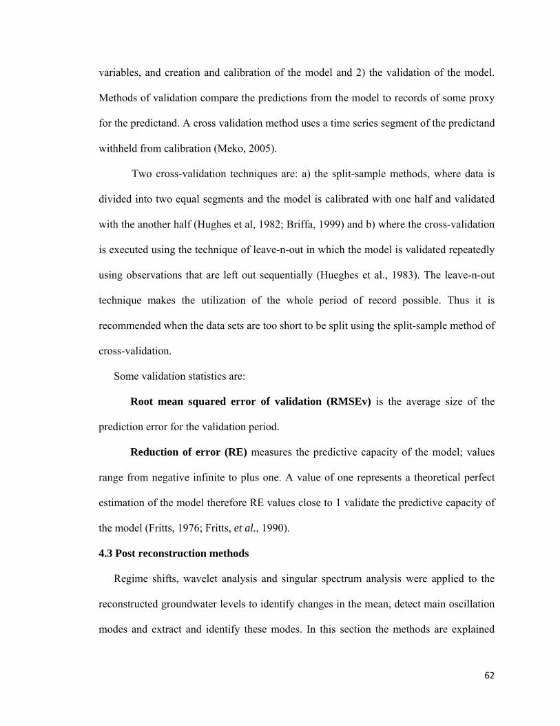
62

variables, and creation and calibration of the model and 2) the validation of the model.

Methods of validation compare the predictions from the model to records of some proxy

for the predictand. A cross validation method uses a time series segment of the predictand

withheld from calibration (Meko, 2005).

Two cross-validation techniques are: a) the split-sample methods, where data is

divided into two equal segments and the model is calibrated with one half and validated

with the another half (Hughes et al, 1982; Briffa, 1999) and b) where the cross-validation

is executed using the technique of leave-n-out in which the model is validated repeatedly

using observations that are left out sequentially (Hueghes et al., 1983). The leave-n-out

technique makes the utilization of the whole period of record possible. Thus it is

recommended when the data sets are too short to be split using the split-sample method of

cross-validation.

Some validation statistics are:

Root mean squared error of validation (RMSEv) is the average size of the

prediction error for the validation period.

Reduction of error (RE) measures the predictive capacity of the model; values

range from negative infinite to plus one. A value of one represents a theoretical perfect

estimation of the model therefore RE values close to 1 validate the predictive capacity of

the model (Fritts, 1976; Fritts, et al., 1990).

4.3 Post reconstruction methods

Regime shifts, wavelet analysis and singular spectrum analysis were applied to the

reconstructed groundwater levels to identify changes in the mean, detect main oscillation

modes and extract and identify these modes. In this section the methods are explained

63

briefly since most of them are complex and advanced. These methods have been

explained and used in many other studies, therefore, for more detail references are cited

and recommended.

4.3.1 Regime shifts

A Regime shift (Rodionov, 2004) method was used to detect significant changes in

mean groundwater levels at the 11 wells reconstructed. Regime shifts is based on

statistical tests and a sequential data processing technique where observations are in time

series and the hypothesis of the existence of a regime shift or discontinuity is tested for

each new observation (Rodionov, 2004).

The method is based on the Student’s test. Rodionov (2004) describes the methods as

follows:

Let x1, x2, ..., xi, ... be a time series with new data arriving regularly. When a new observation arrives, a check is performed to determine whether it represents a statistically significant deviation from the mean value of the “current” regime ( ). According to the t-test, the difference between and the mean value of the new regime ( ) to be statistically significant at the level p should satisfy the conditions

where t is the value of the t-distribution with 2l – 2 degrees of freedom at the given probability level p. It is assumed here that the variances for both regimes are the same and equal to the average variance for running l-year intervals in the time series {xi}. It means that diff remains constant for the entire session with the given time series. At the “current” time tcur , the mean value of the new regime

is unknown, but it is known that it should be equal or greater than the critical level , if the shift is upward, or equal or less than , if the shift is downward, where:

64

If the current value is greater than or less than or less than , the time tcur is marked as a potential change point c, and subsequent data are used to reject or accept this hypothesis. The testing consists of calculating the so-called regime shift index (RSI) that represents a cumulative sum of normalized anomalies relative to the critical level :

If at any time during the testing period from tcur to tcur + l “ 1 the index turns negative, in the case of , or positive, in the case of , the null hypothesis about the existence of a shift in the mean at time tcur is rejected, and the value xcur is included in the “current” regime. Otherwise, the time tcur is declared a change point c.

Regime shifts is a Visual Basic Application (Macro) that is added to Excel and then

used to calculate the shifts in reconstructed mean annual groundwater levels.

4.3.2 Continuous wavelet analysis (CWT)

Wavelet analysis is a relatively new technique in signal processing and can be used on

stationary or non-stationary time series (Daubechies, 1998; Meyer et al., 1993). It locates

the periodic signal in time and identifies the frequency or period (Torrence and Compo,

1998; Jevrejeva et al., 2003).

Continuous wavelet analysis (CWT; Torrence and Compo, 1998; Grinsted et al.,

2004) was used to identify the dominant oscillation modes of variability in groundwater

levels. Among all the wavelet families, Morlet wavelet (w0=6) was chosen and applied to

groundwater levels since it has a good balance between time and frequency domains and

it is recommended when the purpose is to extract quasi-periodic signals (Grinsted et al.

2004). The statistical significance was assessed against a red noise background at 95%.

The Morlet wavelet is defined as follows:

65

Where w0 is dimensionless frequency and µ is dimensionless time.

The application of the convolution theorem to a time series (Xn, n=1,..., N) defines the

continuous wavelet transform (Xn) with uniform time steps . Then, the local phase is

defined by where:

And the wavelet power is defined as .

In order to deal with the cyclic assumption in a wavelet, a cone of influence has been

introduced. This delimits the time domain where edge effects are important (Grinsted et

al., 2004).

Wavelet analysis was carried out in MATLAB using a MATLAB package.To get

more details of the wavelet method used see Torrence and Compo (1998) and Grinsted et

al. (2004)

4.3.3 Singular spectrum analysis (SSA)

Singular spectrum analysis is used to extract information from a short and noisy time

series using principal components techniques (Vautard and Ghil, 1989; Dettinger et al.,

1995). Basically this method extracts the eigenvalues and eigenvectors from the time

series and reconstructs the cyclical components of the time series that are statistically

significant.

66

A description of the method is given by Vautard et al. (1992) is summarized below.

For a time series Xi (i=1, ..., N) and a maximum lag M, the elements of a Toeplitz matrix

are defined by Cj where:

Principal components are calculated to determine the eigenvalues λk and eigenvectors

. Eigenvectors are sorted in decreasing order according their eigenvalue; eigenvalues

greater than 1 are considered statistically significant. The kth principal component is

given by where:

The components of the signal identified by SSA are reconstructed using equation 4.23.

Where is the component reconstructed and represents the addition of one

or more components to the reconstruction.

4.3.4 Percentile analysis

Simple percentile analysis was used in this study to identified periods of low levels in

reconstructed groundwater levels. The time series data are classified by percentiles and

then plotted, generating a barcode to visualize the sequences using colors. For example

67

water levels in the lowest and highest ten percentile will be illustrated with red and blue

respectively.

68

5. RESULTS AND DISCUSSION

This chapter presents results of several methods used to study trends and long term

variability in groundwater levels. It is divided into three main sections which are results

of: trend analysis, groundwater levels reconstructions, and groundwater variability.

5.1 Mann-Kendall trend test

Results of the application of the Mann-Kendall test show that 67% of the wells have a

trend statistically significant at p < 0.05. A decreasing trend is detected in most of the

wells studied (12), and slopes range from -0.5 % to -5.9% (Table 5.1). Increasing trends

were found in 10 groundwater time series, with slopes ranging from 0.7% to 7.5%. No

significant trends were found in the 11 remaining wells studied. The magnitude of

decreasing trends is greater than the rate of increasing trends. For example, a moderate

trend of between 0 and 2 percent applies to 39 percent of the wells with a decreasing

slope in comparison to 60% of the wells with increasing slopes in the same range. For

slopes between 2 and 4 percent the percentages of wells are in the same range for

increasing and decreasing groundwater levels. However, the main difference is where

slopes are greater than 4 percent; in this category there is a 30.5% of the wells with

decreasing trends in comparison with 7% with increasing trends.

Figure 5.1 shows the spatial distribution of the significant (p < 0.05) trends. Central

Alberta is characterized by negative slopes or no trends. In the southern part of the

province some upward and downward trends are found. The trend test results for

Saskatchewan suggest that all the wells studied have significant trends either positive or

negative. Most wells studied in Manitoba present no trend; only one was found to have a

69

significant upward trend. The spatial distribution of trends across the Prairies shows a

distinct pattern, in which northern and central areas are dominated by negative or no

trends, whereas southern areas, in the Prairie Ecozone, show positive trends, with the

notable exception of three wells in or near the forested Cypress Hills.

Table 5.1: Groundwater trends statistics. Slopes entries in bold indicate that they are significant at a 5% level (p < 0.05), * are groundwater levels reconstructed in section 5.2. Name ID Depth Slope Z statistic trend p-value Cressday 85-2 Well 102 80.00 1.3% 5.284 0.000 Pakowki 85-1 Well 104 69.00 3.3% 5.738 0.000 Cypress 85-1 Well 106 30.00 -1.3% -3.708 0.000 Elkwater 2294E Well 108 33.50 3.1% 2.309 0.010 Mud Lake 537E Well 112 36.58 -5.9% -3.988 0.000 Ross Creek 2286E Well 114 73.70 -1.1% -1.819 0.034 Barons 615E * Well 117 19.80 -0.6% -0.081 0.468 Hand Hills #2 South * Well 125 40.54 2.0% 6.119 0.000 Ferintosh Reg Landfill 85-1 Well 147 35.10 -3.0% -2.169 0.015 Devon #2 (North) * Well 159 7.62 0.2% -1.190 0.117 Bruderheim 2340E (S) Well 176 47.90 -0.5% -1.609 0.054 Marie Lake 82-1 Well 192 144.80 0.2% 0.980 0.164 Marie Lake 82-2 (West) Well 193 72.50 0.2% 0.560 0.288 Milk River 85-1 (West) Well 212 73.00 0.8% 1.469 0.071 Kirkpatrick Lake 86-1 (West) Well 228 84.70 -1.8% -4.572 0.000 Kirkpatrick Lake 86-2 (middle) Well 229 33.50 -4.2% -3.419 0.000 Narrow Lake Well 252 26.80 -5.2% -3.337 0.000 Milk River 2479E Well 260 25.90 -0.3% -0.855 0.196 Duvernay 2489E Well 270 20.70 -1.6% -0.855 0.196 Atton * Atto 16.15 -2.7% -7.936 0.000 Baildon 059 B059 30.42 7.5% 5.915 0.000 Bangor A Ban A 39.16 0.8% 4.655 0.000 Bangor B * Ban B 15.27 0.9% 4.657 0.000 Conq 500 C 500 19.16 2.7% 7.112 0.000 Conq 501 * C 501 8.24 2.1% 3.486 0.000 Duck Lake 1 * Duc 1 13.26 -0.6% -3.394 0.000 Duck Lake 2 * Duc 2 124.60 -0.5% -6.537 0.000 Lilac Lila 122.53 1.4% 8.097 0.000 M0-5 OG003 9.14 0.7% 2.393 0.008 Poplarfield #3 LN001 NA 0.0% 0.882 0.189

70

Name ID Depth Slope Z statistic trend p-value

Riceton Rice 22.40 0.6% 8.174 0.000 Sandilands #1 OE001 13.11 -2.9% -1.186 0.118 Simpson 13-04 SI13 7.22 0.2% 1.896 0.029 Smokey A * SmoA 37.12 -3.1% -6.612 0.000 Swanson * Swan 9.18 -2.6% -5.965 0.000 Tyner Tyne 113.69 1.6% 8.214 0.000 Unity * Unit 26.72 1.2% 7.363 0.000 Verlo Verl 12.80 -7.6% -8.191 0.000 Winkler #5 OB005 6.71 -1.2% 0.710 0.239

Figure 5.1: Spatial distribution of trends statistically significant at p<0.05.

Spatial analysis of the magnitude of the slope did not show a spatial pattern, although

groundwater levels in the north central areas dominated by negative trends are minimal in

magnitude (Figure 5.2). As expected from the spatial distribution of trends, the greatest

71

magnitudes are declines in north central areas. On the other hand, even though the slope

of increasing trends mostly do not exceed the 2% there are some areas(i.e. south east

Alberta) dominated by positive slopes between 2-4 percent.

Figure 5.2: Spatial distribution of the slope magnitude for statistically significant trends.

No relationship was found between groundwater levels depth or aquifer lithology and

trends or even the magnitude of the trend.

Spatial comparison between trends in groundwater levels and trends in evaporation

(Burn and Hesh, 2007) suggest that there is spatial coherence between these

hydroclimatic parameters. Trend in evaporation for the warm season (1971-2000) showed

that north central areas of the Canadian Prairies are dominated by no or increasing trends

which is consistent with decreasing groundwater recharge and the results of this study.

72

Assuming that the aquifer recharge is function of precipitation and evaporation, increased

evaporation will lead to decreased recharge (not considering changes in precipitation),

that is reflected by the negative trends that dominate the groundwater levels in north

central areas in the Prairies. Southern areas of the Prairies are dominated by decreasing

trend in evaporation during the warm season (1971-2000) which coincides with the

increasing trends in groundwater domination in this area.

Precipitation in the Canadian Prairies has increased during the last 75 years, although,

this increment is largely rainfall with decreasing snowfall (Akinremi and McGinn,

1999c). No spatial coherence was found between groundwater trends and these changes

in precipitation. Although there might exist a relationship between trends in seasonal

groundwater levels and winter precipitation which has not been explored in this study.

Overall, evaporation rates seem to play a major role in groundwater recharge, even

though, total precipitation has increased in the Prairies there is a significant number of

negative trends in water levels.

The methods used to calculate trends in groundwater levels have been widely used on

stream flow time series with first order autocorrelation. Thus, it would be necessary to

explore the influence of second and third order autocorrelation in the Mann-Kendall trend

test. As it was pointed out in chapter two, groundwater time series generally have

significant autocorrelation of second and third order.

Independent of the methods applied, the use of common periods of time, such as

1971-1990, 1971-2000 and 1981-2000, is recommended. Seasonal and annual trends

73

should be examined in order to make better comparisons with trends in precipitation and

evaporation.

5.2 Tree-ring reconstructions

Using tree-ring chronologies as predictors of groundwater levels, regression models

were built for 11 groundwater wells across Alberta and Saskatchewan. The models

expand annual water level records by more than 300 years in Alberta (Wells 117 and 125)

and for at least 93 years in Saskatchewan. The length of the reconstruction was limited by

the chronologies used in the model where the shortest chronology determines the length

of the reconstruction. Most of the regression models are for wells located in

Saskatchewan where there are longer groundwater records for calibrating the regression

models. As discussed earlier, only three groundwater records in Alberta have the length

and continuity to be used in this study.

In the process of finding the optimal and best reconstruction models for groundwater

levels over 50 models were created (not reported). These models were developed using

different predictors, number of predictors, and positive and negative lags for up to two

years. Selecting the best models was not easy since some regression models presented

better statistics for short periods of reconstruction than for longer periods, which gives

information statistically more reliable. On the other hand, longer reconstructions provide

more information through time but the reliability decreases.

Statistics of the 11 final regression models are presented in table 5.2. All the

models have a positive skill of cross validation indicated by the reduction of error.

74

Residual analysis indicates that most of the regression models did not have significant

autocorrelation in the residuals. The Durbin-Watson statistic was in the uncertain range

for three regression models (Duc1, Duc2, and Swan). In statistical terms the best

reconstruction model explains 82% of the instrumental variance in annual groundwater

levels for the Unit observation well; in contrast, the regression model for well Duck Lake

1 explains the lowest percent of variance (40%). Other models in Saskatchewan explain

high amounts of variance (over 70%). Even though intuitively tree growth driven by soil

moisture should correlate best with shallow groundwater levels, the statistics obtained

from the regression model for the deepest groundwater record reconstructed in this study,

Duck Lake 2 (Duc2), are better than for a few shallow wells, which suggests the possible

utilization of tree growth to reconstruct groundwater levels in deep aquifers.

In terms of length, Alberta models allowed reconstruction of groundwater levels for

up to 387 years (w117) which even exceeds some tree-ring reconstructions of stream flow

and precipitation in the area (Watson and Luckman, 2001; Case and McDonald, 2003;

Axelson, 2007) . The shortest reconstruction, but the best in terms of instrumental

variance explained, is well 159. Also, this is the only model has tree-ring variables with

positive and negative lags as predictors. This shortest reconstruction for Alberta exceeds

the longest reconstruction in Saskatchewan.

75

Table 5.2: Statistics of the optimal regression models

Name Period Length

(yrs) Calibration

Period Lag

# of Predictors

R2 R2 adj

RE SE AC1 Max VIF

w 117 1618-2003 387 1972-2003 0 3 0.73 0.71 0.640 0.57480 H0 2.8

w125 1684-2003 320 1973-2003 0 6 0.60 0.52 0.360 0.70470 H0 5.5

w159 1859-2002 144 1968-2001 ±2 7 0.80 0.76 0.630 0.46630 H0 1.7

Atto 1879-2001 123 1966-2001 0 5 0.81 0.79 0.730 0.41263 H0 5.5

Ban B 1909-2001 93 1971-2001 0 4 0.77 0.75 0.580 0.48250 H0 1.5

C 501 1862-2001 140 1972-2001 0 4 0.61 0.56 0.450 0.28390 H0 2.5

Duc 1 1909-2001 93 1967-2001 0 5 0.47 0.40 0.270 0.63710 U 1.6

Duc 2 1875-2001 127 1966-2001 0 5 0.74 0.71 0.640 0.05510 U 2.8

Smoa 1879-2001 123 1971-2001 0 5 0.80 0.77 0.690 0.15130 H0 4.5

Swan 1875-2001 127 1972-2001 0 4 0.67 0.63 0.520 0.62110 U 1.6

Unit 1875-2001 127 1968-2001 0 2 0.82 0.81 0.780 0.09890 H0 1.5

H0: No first order autocerrelation in residual. U: Uncertain

One important assumption in linear regression modeling is the normality of the

predictands. The normality test showed that most mean annual groundwater levels are not

normally distributed and therefore they need to be transformed. Common and widely

used transformations in hydrological time series did not work on groundwater levels

hence the complex Johnson transformation was used. Once the time series were

transformed they were tested for normality again. The results of this second test showed

that the Johnson transformation succeeded one hundred percent. Transformation and

linear regression equations are listed in Table 5.3.

Table 5.3: Transformation and regression equations

Well Johnson transformed Linear regression model

w117 1.33505 + 0.977974*Asinh[(x-962.543) / 0.147662]

0.5128 + 2.2440*DBY - 1.8548*WLPG + 2.5679*FIL - 4.4372*ILK

w125 -0.422957 + 0.580869*Asinh[(x-978.919) / 0.0460879]

3.5958 + 1.3604*WCH - 1.8532*SIP + 1.5203*OK24 - 1.9671*OCPC - 1.9214*DCK - 1.3258*BSG

w159 1.60130 + 1.40428*Asinh[(x-691.530) / 0.230649]

-2.2684 + 1.3660*WCH-1 - 2.3403*OCPC-1 + 4.0188*H88-1 - 1.2779*SW-2 + 1.6914*H88+1 + 3.1735*SW2+2 - 4.1839*FLK+2

Atto 1.79953 + 1.94815*Asinh[(x-528.362) / 0.376]

-0.6029 - 1.2790*KIL + 3.3523*ORP - 1.9445*FBY - 1.0310*MLK + 1.8361*WLPB

BanB 0.241646 + 0.587977*Ln[(x- -1.0863 - 1.6735*ILK - 2.1332*CHPC + 2.1463*DEV +

76

Well Johnson transformed Linear regression model 514.436) / (515.133-x)] 2.36836*ILL

C501 No 565.9887 + 0.7104*DBY - 0.946*WLPG + 0.6886*WLPB + 1.1463*DEV

Duc1 0.295628 + 1.08316*Asinh[(x-499.249) / 0.187576]

-0.6089 + 1.7761*ORP + 1.5138*FIL - 2.6282*CHPC + 1.4661*DEV - 1.4543*HILL

Duc2 No 479.1639 - 0.1535*DBY + 0.2077*FBY + 0.5481*FIL - 0.2832*ILK - 0.2702*MLK

SmoA No 303.3906 + 1.0191*ORP + 0.3268*WLPG - 0.5081*FBY - 0.2264*FIL - 0.4572*DEV

Swan 0.515740 + 0.526811*Ln[(x-528.487) / (529.576-x)]

-2.0288 + 1.3115*KIL + 1.7886*WLPG + 2.4068*ILK - 2.8036*CHPC

Unit 2.35697 + 0.990162*Asinh[(x-656.946) / 0.0209937]

0.5128 + 2.2440*DBY - 1.8548*WLPG + 2.5679*FIL - 4.4372*ILK

5.2.1 Calibration of Alberta models

Plots of observed and reconstructed groundwater levels are shown below for wells

117, 125, and 159 (Fig. 5.3, 5.4, and 5.5, respectively). The models capture a large part of

the inter-annual variability for wells 117 and 159 following a similar pattern. In general,

these two models estimate well extreme groundwater levels. The regression model for

well 117 initially overestimates water levels but then is in-phase with observed water

levels until the 1980s; the models underestimate water levels in late 1980s and 1990s

(Fig. 5.3). Well 159 underestimates water levels at the beginning of the record and

reconstructs greater inter annual variability than observed from the late 1970s until late

1980s. Afterwards low and high levels are well estimated excluding the low level in the

late 1980s (Fig. 5.4). As stated before, the regression model for well 125 has the worst

statistics of the three models as evident in Figure 5.5. The model gives greater inter

annual variability than the water levels observed that seem to be driven by an inter-

decadal climate variability; however, the model is picking up relatively well low and high

levels. Generally, it is overestimating the lows excepting water levels in 2000.

77

1970 1975 1980 1985 1990 1995 2000

-2

-1

0

1

2

3

Gro

un

dw

ate

r le

vel

tr

ansf

orm

ed (

w11

7) R2=0.73 R2adj=0.71 RE=0.64

Figure 5.3: Calibration period for well 117. Blue and red lines are groundwater levels reconstructed and observed respectively.

1970 1975 1980 1985 1990 1995 2000

-2

-1

0

1

2

Gro

un

dw

ater

lev

eltr

an

sfo

rmed

(w

125) R2=0.60 R2

adj=0.52 RE=0.36


1965 1970 1975 1980 1985 1990 1995 2000

-3

-2

-1

0

1

2

3

Gro

un

dw

ate

r le

vel

tra

nsf

orm

ed (

w15

9)

R2=0.80 R2adj=0.76 RE=0.63


78

5.2.1.1 Tree-ring reconstructions of groundwater levels in Alberta

The use of tree-rings makes possible the reconstruction of historical groundwater

levels at three observation wells in Alberta (Wells 117, 125, and 159). The regression

models expand water level records by 387, 320, and 144 years at wells 117, 125, and 159,

respectively. Consecutive years of low and high water levels are identified in each of the

reconstructions.

The 387-year reconstruction for well 117 shows periods of persistent low and high

water levels (Figure 5.6). Major lows are centered on 1698, 1720, 1859, 1920, 1944, and

1985. On the other hand, major highs are centered on 1775, 1825, 1910 and 1975. From

smoothing (15 years running average) the reconstructed time series, the period centered

on 1859 represents the lowest water levels for the longest period, although the shorter

periods centered on 1969, 1720, and 1985 had years with lower water levels than the

interval of prolonged low levels centered on 1859. During the last 250 years, a clearly

inter-decadal variability and decreasing in water levels are observed in the reconstruction.

Table 5.4 summarizes water levels below the 30th percentile. Under this classification

there are five periods of five or more consecutive years in which water level are below 30

percent. Also this table shows the 15 years with the lowest water levels; five of these

years were in the last 20 years.

79

-2

-1

0

1

2

3

GWL reconstructed

(w117)

1600 1650 1700 1750 1800 1850 1900 1950 2000

1600 1650 1700 1750 1800 1850 1900 1950 2000

Percentile (P) ClassesP < 10

10 < P < 20

20 < P < 40

40 < P < 60

60 < P < 80

80 < P < 100

R2adj=0.71 RE=0.64

Figure 5.6: Groundwater levels reconstructed at well 117 and the 15-year running mean (grey and black lines respectively). At the bottom is the bar code representing percentile classes of groundwater levels.

Groundwater level reconstructed at well 125 shows less clearly inter-decadal

variability (Figure 5.7). Low and high levels are identified, however, the pattern is more

diffuse. Fewer periods of extreme low levels are identified, although the longest and most

extreme low level period is seen in this reconstruction (~1925-1966). Some high levels

are centered on 1775, 1815, and 1875. The least extreme relatively high period, centered

on 1910, is followed by decreasing water levels and 40 years of the lowest water levels in

the 320 years. Seven of the lowest annual water levels are found in this period (Table

5.5). As with well 117, before 1750s water levels show less variability (a relatively stable

15-year running average).

80

1650 1700 1750 1800 1850 1900 1950 2000

-3

-2

-1

0

1

2

GWL reconstructed

(W125)

1650 1700 1750 1800 1850 1900 1950 2000


10 < P < 20

20 < P < 40

40 < P < 60

60 < P < 80

80 < P < 100

R2adj=0.52 RE=0.36


Mostly one or two consecutive years with low levels are identified in the

reconstruction at well 159. The longest period of consecutive years (5) is centered on

1970. There are other periods of low level, such as the one centered on 1920, that include

a few years of high levels. The inter-decadal variability is also seen but not to the same

degree as previously. High levels are centered on 1870, 1940 and 1960 (Fig. 5.8). The

period centered on 1980 is relatively stable showing less variability.

81

1840 1860 1880 1900 1920 1940 1960 1980 2000

-4

-2

0

2

4

GW

L r

eco

nst

ruc

ted

(W15

9)

1840 1880 1920 1960 2000


10 < P < 20

20 < P < 40

40 < P < 60

60 < P < 80

80 < P < 100

R2adj=0.76 RE=0.63


Nkemedirin and Weber (1999) compared the 1930s and 1980s droughts. The 1930s

drought was characterized as the driest and more prolonged drought of the two, although

winter and springs were wetter than normal while during the 1980s drought winter and

spring precipitation was below average. In both there were dry summers. The impact of

these droughts on groundwater levels vary at the different wells studied. The 1930s

drought had a stronger impact on water levels at wells 125 and 159 than at well 117. This

drought had as a consequence low water levels at well 125 for more than 40 years which

is probably related to aquifer conditions and the longer period of recovery for deeper

aquifers. During this period water levels were mostly in the lowest 20 percent, the lowest

water levels reconstructed occurred during this period. The major impact of the 1930s

drought can be attributed to the high evaporation rate during this decade. This highlight

the impact of evaporation on groundwater levels during the warm season (seen previously

82

in trends).On the other hand, the 1980s drought produced greater impacts on water levels

at well 117 than at the other sites.

Some other common periods of low surface water levels have been previously

recognized for the Canadian Prairies, for example the period centered on 1860 (St.

George and Nielsen, 2002), This dry period had the strongest and longest impacts on

groundwater levels at well 117 (Fig. 5.6b).

Table 5.4: Groundwater levels < 30th percentile at Well 117 (1618-2003). Bold entries indicate groundwater levels < 10th percentile. Asterisks indicate years during the last two major droughts in the Canadian Prairies.

Single Year More than 2 and less than 5 years

5 or more consecutive years

Lowest GWL (increasing order)

1630,1634,1650,1681,1702,1706,1711,1736,1748,1753,1800,1840,1842,1883,1893,1896,1910,1917,1926,1948,1956,1980,2000

1663,1664,1665

1696,1697,1698,1699,1700

1760,1634,1988*,1722,1989*,1696,1865,1697,2000*,1718, 1723,1990*,1698,1785,1720

1687,1688 1718,1719,1720,1721,1722,1723

1690,1691 1853,1854,1855,1856,1857,1858,1859 1708,1709

1730,1731,1732 1861,1862,1863,1864,1865,1866,1867 1758,1759,1760,1761

1763,1764 1983,1984,1985,1986,1987,1988,1989,1990,1991,1992 1785,1786,1787

1792,1793,1797 1812,1813 1817,1818 1830,1831 1844,1845,1846 1848,1849 1870,1871,1872 1875,1876,1877 1889,1890 1919,1920,1921,1922 1936,1937 1940,1941 1943,1944,1945,1946 1961,1962,1963

83

Table 5.5: Groundwater levels < 30th percentile at Well 125 (1684-2003). Bold entries indicate groundwater levels < 10th percentile. Asterisks indicate years during the last two major droughts in the Canadian Prairies. Single year More than 2 and less than 5

years 5 or more consecutive years


1692,1697,1708,1717,1720,1727,1747,1756,1758,1761,1768,1796,1799,1801,1808,1850,1868,1881,1914,1916,1918,1970,1973

1699,1700

1898,1899,1900,1901,1902

1900,1938,1935,1943,1936,1901,1700,1957,1958,1806,1953,1963,1805,1740,1951

1704,1705 1924,1925,1926,1927,1928,1929,1930,1931,1932,1933,1934,1935,1936,1937,1938,1939,1940,1941,1942,1943,1944,1945,1946

1711,1712 1723,1724 1738,1739,1740,1741

1749,1750 1804,1805,1806 1948,1949,1950,1951,1952,

1953,1954,1955 1828,1829

1855,1856 1962,1963,1964,1965,1966 1885,1886

1890,1891 1904,1905,1906 1957,1958,1959 1992-93

Table 5.6: Groundwater levels < 30th percentile at Well 159 (1859-2002). Bold entries indicate groundwater levels < 10th percentile. Asterisks indicate years during the last two major droughts in the Canadian Prairies. Single year More than 2 and less than 5



1868,1870,1882,1885,1890,1892,1900,1911,1913,1917,1926,1937,1945,1947,1949,1995,2001

1859,1860

1968,1969,1970,1971,1972

1924,1931,1932,2001*,1885,1919,1890,1908, 1926,1859,1906,1911, 1887,1945,1920

1863,1864,1879,1880 1887,1888 1906,1907,1908 1919,1920 1922,1923,1924 1931,1932 1957,1958 1988,1989

5.2.2 Calibration Saskatchewan

As in Alberta, regression models in Saskatchewan show a greater inter-annual

variability than observed groundwater records, although they show a relatively similar

pattern.

84

The calibration period for well Atto (Fig. 5.9) shows that observed and reconstructed

groundwater levels have a decreasing trend. There is some under estimation of low and

high water levels in the early 1980s and 1990s. Overall the model captures well low and

high water levels and the model explains 79% of the instrumental variance. Regression

models for wells BanB and C501explain 75% and 56% of the instrumental variance

respectively. Both of them underestimate water levels in the early 1990s and after that

show an increasing trend that coincides with observed water levels (Fig. 5.10 and 5.11).

Duc1, as pointed out before is the worst of the regression models in statistical terms

explaining just 40% of the instrumental variance (Fig. 5.12). The under and

overestimation plus the out of phase peaks account for the unexplained variance. Water

levels at Duc2 show a continuously increasing trend from 1965 to 1976 afterwards

decrease. This pattern is captured by the regression model which explains 71% of the

instrumental variance. The model has two clear overestimations of water levels in the

early 1970s and 1990s (Fig. 5.13). Regression models for wells SmoA and Swan explain

77% and 63% of the instrumental variance. Both models follow the decreasing trend of

water levels but show a certain degree out of phase especially for high water levels (Fig.

5.14 and 5.15). Overestimation of low levels in the early 1990s is evident in the model for

well Swan. Finally, the best regression model in statistical terms is for water levels at

well Unit. This model explains 82% of the instrumental variance and has the longest

calibration period (1966-2001). The increasing trend is followed by the model adding

some inter-annual variability that is not seen in the well record. It captures high and low

levels relatively well; however, there is an underestimation of high water levels in late

1990s (Fig. 5.16).

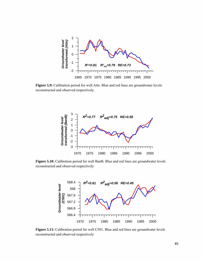
85

1965 1970 1975 1980 1985 1990 1995 2000

-2

-1

0

1

2

Gro

un

dw

ate

r le

vel

tra

ns

form

ed (

Att

o)

R2=0.81 R2adj=0.79 RE=0.73

Figure 5.9: Calibration period for well Atto. Blue and red lines are groundwater levels reconstructed and observed respectively.

1970 1975 1980 1985 1990 1995 2000

-3

-2

-1

0

1

2

3

Gro

un

dw

ater

leve

ltr

ansf

orm

ed

(B

an

B)

R2=0.77 R2adj=0.75 RE=0.58

Figure 5.10: Calibration period for well BanB. Blue and red lines are groundwater levels reconstructed and observed respectively

1970 1975 1980 1985 1990 1995 2000

566.4

566.8

567.2

567.6

568

568.4

Gro

un

dw

ate

r le

vel

(C5

01)

R2=0.61 R2adj=0.56 RE=0.45

Figure 5.11: Calibration period for well C501. Blue and red lines are groundwater levels reconstructed and observed respectively

86

1965 1970 1975 1980 1985 1990 1995 2000

-2

-1

0

1

2

Gro

un

dw

ate

r le

vel

tra

ns

form

ed (

Du

c1)

R2=0.47 R2adj=0.40 RE=0.27

Figure 5.12: Calibration period for well Duc1. Blue and red lines are groundwater levels reconstructed and observed respectively

1965 1970 1975 1980 1985 1990 1995 2000

479

479.1

479.2

479.3

479.4

479.5

Gro

un

dw

ate

r le

vel

(Du

c2)

R2=0.74 R2adj=0.71 RE=0.64

Figure 5.13: Calibration period for well Duc2. Blue and red lines are groundwater levels reconstructed and observed respectively

1970 1975 1980 1985 1990 1995 2000

302.8

303.2

303.6

304

304.4

Gro

un

dw

ater

lev

el(S

mo

A)

R2=0.80 R2adj=0.77 RE=0.69

Figure 5.14 Calibration period for well SmoA. Blue and red lines are groundwater levels reconstructed and observed respectively

87

1970 1975 1980 1985 1990 1995 2000

-3

-2

-1

0

1

2

3

Gro

un

dw

ater

leve

ltr

ansf

orm

ed

(S

wa

n)

R2=0.67 R2adj=0.63 RE=0.52

Figure 5.15: Calibration period for well Swan. Blue and red lines are groundwater levels reconstructed and observed respectively

1965 1970 1975 1980 1985 1990 1995 2000

-3

-2

-1

0

1

2

Gro

un

dw

ater

lev

el

tra

ns

form

ed

(U

nit

) R2=0.83 R2adj=0.82 RE=0.78

Figure 5.16: Calibration period for well Unit. Blue and red lines are groundwater levels reconstructed and observed respectively

5.2.2.1 Tree-ring reconstructions of groundwater levels in Saskatchewan

The groundwater level reconstructions show a similar pattern of low and high levels

for wells Atto, BanB C501, SmoA and Unit; high water levels are centered around the

1950s (Figures 5.17, 5.18, 5.19, 5.22, and 5.24). Another similar period centered on 1970

was detected at wells Atto, Duc2, SmoA and Swan (Figures 5.17, 5.21, 5.22, 5.23).

Common periods of low water levels are reconstructed in the late 1880s, late 1920s

and early 1930s at well Atto, where low levels are followed by high levels for around 20

88

yr (1941-1962), at well C501 where ~10 years are dominated by low levels, and at wells

BanB, Duc1, Duc2, SmoA and Unit. During these periods water levels at Swan dropped

but not as much as in the rest of the wells. Water levels were low in the early 1960s at

wells BanB, C501, Duc2 and Unit extending for around 20 consecutive years (1951-

1971). Wells Atto, BanB, C501, Duc1, SmoA and Swan had low levels during or shortly

following the drought in 1988. Also, effects of the 2000-01 drought are observed on Atto,

Duc1, Smoa, and Swan water levels, which have been decreasing since the late 1960s.

1880 1900 1920 1940 1960 1980 2000

-2

-1

0

1

2

3

4

GW

L r

eco

ns

tru

cte

d(A

tto

)

1880 1900 1920 1940 1960 1980 2000


10 < P < 20

20 < P < 40

40 < P < 60

60 < P < 80

80 < P < 100

R2adj=0.79 RE=0.73

Figure 5.17: Groundwater levels reconstructed at well Atto and the 15-year running mean (grey and black lines respectively). At the bottom is the bar code representing percentile classes of groundwater levels.

89

1900 1910 1920 1930 1940 1950 1960 1970 1980 1990 2000

-4

-2

0

2

4

GW

L r

eco

nst

ruc

ted

(Ba

nB

)

1910 1920 1930 1940 1950 1960 1970 1980 1990 2000


10 < P < 20

20 < P < 40

40 < P < 60

60 < P < 80

80 < P < 100

R2adj=0.75 RE=0.58

Figure 5.18: Groundwater levels reconstructed at well BanB and the 15-year running mean (grey and black lines respectively). At the bottom is the bar code representing percentile classes of groundwater levels.

1860 1880 1900 1920 1940 1960 1980 2000

566

567

568

569

570

GW

L r

eco

nst

ruc

ted

(C50

1)

1860 1880 1900 1920 1940 1960 1980 2000


10 < P < 20

20 < P < 40

40 < P < 60

60 < P < 80

80 < P < 100

R2adj=0.56 RE=0.45

Figure 5.19: Groundwater levels reconstructed at well C501 and the 15-year running mean (grey and black lines respectively). At the bottom is the bar code representing percentile classes of groundwater levels.

90

1900 1910 1920 1930 1940 1950 1960 1970 1980 1990 2000

-2

-1

0

1

2

3

GW

L r

eco

nst

ruct

ion

(Du

c1)

1910 1920 1930 1940 1950 1960 1970 1980 1990 2000


10 < P < 20

20 < P < 40

40 < P < 60

60 < P < 80

80 < P < 100

R2adj=0.40 RE=0.27

Figure 5.20: Groundwater levels reconstructed at well Duc1 and the 15-year running mean (grey and black lines respectively). At the bottom is the bar code representing percentile classes of groundwater levels.

1880 1900 1920 1940 1960 1980 2000

478.8

479

479.2

479.4

479.6

479.8

GW

L r

eco

nst

ruc

ted

(Du

c2)

1880 1900 1920 1940 1960 1980 2000


10 < P < 20

20 < P < 40

40 < P < 60

60 < P < 80

80 < P < 100

R2adj=0.71 RE=0.64

Figure 5.21: Groundwater levels reconstructed at well Duc2 and the 15-year running mean (grey and black lines respectively). At the bottom is the bar code representing percentile classes of groundwater levels.

91

1880 1900 1920 1940 1960 1980 2000

302.8

303.2

303.6

304

304.4

GW

L r

eco

nst

ruc

ted

(Sm

oA

)

1880 1900 1920 1940 1960 1980 2000


10 < P < 20

20 < P < 40

40 < P < 60

60 < P < 80

80 < P < 100

R2adj=0.77 RE=0.69

Figure 5.22: Groundwater levels reconstructed at well SmoA and the 15-year running mean (grey and black lines respectively). At the bottom is the bar code representing percentile classes of groundwater levels.

1880 1900 1920 1940 1960 1980 2000

-2

-1

0

1

2

3

GW

L r

eco

nst

ruc

ted

(Sw

an)

1880 1900 1920 1940 1960 1980 2000


10 < P < 20

20 < P < 40

40 < P < 60

60 < P < 80

80 < P < 100

R2adj=0.63 RE=0.52

Figure 5.23: Groundwater levels reconstructed at well Swan and the 15-year running mean (grey and black lines respectively). At the bottom is the bar code representing percentile classes of groundwater levels.

92

1880 1900 1920 1940 1960 1980 2000

-6

-4

-2

0

2

4

GW

L r

eco

nst

ruc

ted

(Un

it)

1880 1900 1920 1940 1960 1980 2000


10 < P < 20

20 < P < 40

40 < P < 60

60 < P < 80

80 < P < 100

R2adj=0.82 RE=0.78

Figure 5.24: Groundwater levels reconstructed at well Unit and the 15-year running mean (grey and black lines respectively). At the bottom is the bar code representing percentile classes of groundwater levels.

Years with water levels in the lowest thirty percentile are summarized by Tables 5.7-

5.14. Up to three periods of five or more consecutive years with low levels were

reconstructed at wells BanB, Duc2, Swan and Unit during the last century. Several

periods with more than two, and less than five, years of low levels are identified where

droughts had taken place in the last century. Also, the top 15 years with the lowest water

levels are presented in these tables. Only a few years of instrumental records are in this

group which suggests that groundwater levels were lower when there is no instrumental

record, although four of the 15 lowest water levels occurred during the last 10 years at

well Atto and the period 1998-2001 is among the six lowest water levels in 123 years.

93

Table 5.7: Groundwater levels < 30th percentile at Well Atto. Bold entries indicate groundwater levels < 10th percentile. Asterisks indicate years during the last two major droughts in the Canadian Prairies. Single year More than 2 and less than 5



1886, 1893, 1896, 1899, 1904, 1907, 1916, 1923, 1934, 1940, 1963, 1990

1881, 1882, 1883, 1884 1995, 1996, 1997, 1998, 1999, 2000, 2001

1882, 2001*, 2000*, 1914, 1998*, 1999*, 1916, 1896, 1925, 1997*, 1921, 1930, 1881, 1886, 1934

1913, 1914

1919, 1920, 1921

1925, 1926, 1927

1929, 1930, 1931

1981, 1982, 1983

Table 5.8: Groundwater levels < 30th percentile at Well BanB Bold entries indicate groundwater levels < 10th percentile. Asterisks indicate years during the last two major droughts in the Canadian Prairies. Single year More than 2 and less than 5



1915, 1926, 1970, 1987

1921, 1922, 1923 1929, 1930, 1931, 1932, 1933, 1934

1963, 1931, 1940, 1922, 1932, 1964, 1965, 1939, 1930, 1961, 1966, 1960, 1941, 1933, 1923

1990, 1991, 1992 1937, 1938, 1939, 1940, 1941, 1942 1960, 1961, 1962, 1963, 1964, 1965, 1966

Table 5.9: Groundwater levels < 30th percentile at Well C501 . Bold entries indicate groundwater levels < 10th percentile. Asterisks indicate years during the last two major droughts in the Canadian Prairies. Single year More than 2 and less than 5



1896, 1903, 1929, 1931, 1940, 1972, 1974, 1977

1877, 1878 1870, 1871, 1872, 1873, 1874, 1875

1896, 1931, 1982*, 1962, 1961, 1872, 1874, 1873, 1963, 1918, 1922, 1892, 1903, 1878

1884, 1885 1979, 1918, 1919, 1920, 1921, 1922 1891, 1892, 1893

1913, 1914, 1915

1937, 1938

1960, 1961, 1962, 1963

1980, 1981, 1982

1988, 1989

94

Table 5.10: Groundwater levels < 30th percentile at Well Duc1 Bold entries indicate groundwater levels < 10th percentile. Asterisks indicate years during the last two major droughts in the Canadian Prairies. Single year More than 2 and less than 5



1909, 1938, 1940, 1947, 1950, 1952, 1959, 1968, 1988, 1990, 1993

1915, 1916 1926, 1927, 1928,

1929, 1930, 1931

1952, 1962, 1915, 1916, 1931, 1929, 1909, 1998*, 2000*, 1940, 1923, 1947, 1990*, 1943, 1999*

1923, 1924

1943, 1944

1961, 1962

1998, 1999, 2000, 2001

Table 5.11: Groundwater levels < 30th percentile at Duc2 . Bold entries indicate groundwater levels < 10th percentile. Asterisks indicate years during the last two major droughts in the Canadian Prairies. Single year More than 2 and less than

5 years 5 or more consecutive years Lowest GWL

(increasing order)

1882, 1893, 1897, 1924, 1940

1935, 1936, 1937 1884, 1885, 1886, 1887, 1888 1961, 1929, 1928, 1954, 1886, 1955, 1958, 1963, 1893, 1953, 1962, 1960, 1959, 1885, 1956

1943, 1944, 1945, 1946 1926, 1927, 1928, 1929, 1930

1950, 1951, 1952, 1953, 1954, 1955, 1956, 1957, 1958, 1959, 1960, 1961, 1962, 1963, 1964, 1965, 1966

Table 5.12: Groundwater levels < 30th percentile at SmoA. Bold entries indicate groundwater levels < 10th percentile. Asterisks indicate years during the last two major droughts in the Canadian Prairies. Single year More than 2 and less than


(increasing order)

1896, 18991919, 1923, 1964, 1995

1879, 1880, 1881, 1882 1881, 2000*, 1999*, 1882, 1990*, 2001*, 1923, 1916, 1998*, 1991*, 1993*, 1915, 1931, 1927, 1926

1911, 1912

1914, 1915, 1916

1925, 1926, 1927

1929, 1930, 1931

1938, 1939, 1940

1984, 1985

1987, 1988

1990, 1991, 1992, 1993

1998, 1999, 2000, 2001

95

Table 5.13: Groundwater levels < 30th percentile at Swan. Bold entries indicate groundwater levels < 10th percentile. Asterisks indicate years during the last two major droughts in the Canadian Prairies. Single year More than 2 and less than


(increasing order)

1927, 1939 1877, 1878 1907, 1908, 1909, 1910, 1911, 1912, 1913

1943, 1915, 1909, 1908, 1991, 1995, 1942, 1907, 1916, 1993, 1990*, 1877, 1944, 1999*, 1912

1899, 1900, 1901

1915, 1916 1941, 1942, 1943, 1944, 1945, 1946, 1947, 1948 1981, 1982

1998, 1999, 2000 1987, 1988, 1989, 1990, 1991, 1992, 1993, 1994, 1995, 1996

Table 5.14: Groundwater levels < 30th percentile at Well Unit Bold entries indicate groundwater levels < 10th percentile. Asterisks indicate years during the last two major droughts in the Canadian Prairies. Single year More than 2 and less than


(increasing order)

1882 1929, 1930, 1931 1884, 1985, 1986, 1987, 1988 1963, 1961, 1960, 1964, 1922, 1966, 1884, 1965, 1954, 1957, 1962, 1929, 1921, 1955, 1930

1936, 1937, 1938 1920, 1921, 1922, 1923, 1924, 1925, 1926

1950, 1951 1953, 1954, 1955, 1956, 1957, 1958, 1959, 1960, 1961, 1962, 1963, 1964, 1965, 1966, 1967

1969, 1970, 1971

As with the reconstruction of groundwater in Alberta, the models in Saskatchewan

reflect changes in mean annual groundwater levels forced by climate, as recorded by trees

in Alberta and Saskatchewan.

Tree-ring reconstructions suggest that the range of water levels observed during the

last 45 years does not reflect the natural variation in groundwater levels.

5.2.3 Statistical comparison between observed and reconstructed groundwater levels

The main statistics of reconstructed and observed groundwater levels are summarized

in Table 5.15. Mean water level for the 1618-2003 at well 117 is higher than recorded

over the period of instrumental observations (1972-2003), although the minimum and

96

maximum water levels are lower than the minimum record and the maximum recorded.

On the other hand, mean water levels for the periods of 1684-2003 and 1859-2002 at

wells 125 and 159 respectively are lower than the recorded over the period of

instrumental observations (1973-2003; 1968-2001). Minimum and maximum

reconstructed water levels are lower than minimum and maximum observed which

suggest the existence of more extreme dry events driving low water levels.

In Saskatchewan, mean water levels for the periods of 1879-2001, 1862-2001,1879-

2001, 1875-2001 at wells Atto, C501, SmoA and Swan are higher than means recorded

over the periods of 1966-2001, 1972-2001, 1971-2001, and 1972-2002 respectively.

Minimum water levels were lower at wells Atto and C501 and higher at wells SmoA and

Swan during the reconstruction period than during the instrumental period. At wells

BanB, Duc1, Duc2, and Unit mean reconstructed water levels (1909-2001-;1909-

2001;1872-2001;1872-2001) are lower than the instrumental means recorded (1971-

2001;1967-2001;1966-2001;1968-2001). Minimum and maximum reconstructed water

levels are lower and higher than minimum and maximum water levels recorded at the 4

wells.

Table 5.15: Statistical comparison between observed and reconstructed water levels Well Mean StDev Variance Median Minimum Maximum Range N

w117 -0.00239 1.03188 1.06479 -0.12732 -1.54309 2.81647 4.35956 34

w117_rec 0.13301 0.76670 0.58784 0.15074 -1.98388 2.71032 4.69421 386

w125 0.03808 1.00591 1.01186 0.06102 -1.93106 1.49967 3.43073 32

w125_rec -0.49778 0.80240 0.64384 -0.46918 -2.68069 1.44462 4.12531 320

w159 0.16931 0.92933 0.86365 0.08566 -1.27557 2.63087 3.90644 34

w159_rec 0.11400 1.03975 1.08108 0.16483 -2.59469 2.59495 5.18964 144

Atto 0.15998 0.88505 0.78332 0.13195 -1.41518 1.83135 3.24652 36

Atto_rec 0.25170 0.94714 0.89708 0.01946 -1.79419 3.00877 4.80295 123

BanB -0.12520 0.94450 0.89208 -0.31177 -2.19437 2.13829 4.33265 31

BanB_rec -0.42150 1.22129 1.49154 -0.52899 -2.82959 3.95813 6.78772 93

97

Well Mean StDev Variance Median Minimum Maximum Range N

C501 567.476 0.420 0.176 567.450 566.742 568.237 1.494 30

C501_rec 567.558 0.473 0.224 567.460 566.279 569.196 2.917 140

Duc1 0.12054 0.80878 0.65412 -0.18121 -1.27608 1.82438 3.10046 35

Duc1_rec 0.07908 0.69442 0.48221 0.03896 -1.40956 2.26670 3.67626 93

Duc2 479.276 0.100 0.010 479.263 479.108 479.460 0.352 36

Duc2_rec 479.214 0.128 0.016 479.210 478.957 479.630 0.673 127

SmoA 303.496 0.311 0.097 303.452 302.975 304.119 1.144 31

SmoA_rec 303.533 0.248 0.061 303.492 303.013 304.195 1.182 123

Swan 0.12505 1.00740 1.01485 0.23036 -2.22000 2.22000 4.44000 30

Swan_rec 0.60553 1.02680 1.05431 0.60310 -1.47448 2.82553 4.30001 127

Unit -0.10685 1.08238 1.17155 -0.14776 -1.88141 1.96650 3.84791 34

Unit_rec -0.83108 1.28877 1.66092 -0.83686 -4.05640 2.78023 6.83662 127

5.3 Analyses post reconstruction: Regime shifts, wavelets and singular spectrum

analysis

The utilization of regime shifts analysis to detect shifts in the mean, plus wavelet and

singular spectrum analysis (SSA) is a powerful combination to analyze the variability of

groundwater levels and enable the identification and attribution of the major changes in

mean water levels.

5.3.1 Alberta

Results of the regime shifts analysis suggest that there have been constant changes in

mean groundwater levels at well 117 (Fig. 5.25a). Several periods of higher and lower

water levels than average are identified from the reconstruction. There are more periods

above average than below, although, periods below average are longer.

98

There are two major periods with low levels: a 36 year period starting in 1842 and a

35 year period starting in 1914. Also a third relatively long period of low water levels

starts in 1979 and extends to 1991.

Result of wavelet analysis show significant activity in the 3-6, 6-12, and around 64

year bands (Fig. 5.25b). Most of the activity in the 2-6 yr band occurs in the period 1850-

2000. Significant activity in the 6-12 yr band occurs in the early and late 1700s. The ~64

year band presents significant activity from the first quarter of the eighteen century which

coincides with the first period of low levels.

Singular spectrum analysis is used to separate different oscillation modes detected by

wavelet analysis. Six major waveforms at 6.4, 9.69, 10.8, 14.2, 24.5, and 66.3 years were

isolated from the groundwater reconstruction (Fig. 5.25c). These six oscillation modes

account for 51.5% of the total variance in the reconstruction. Most of the modes

identified by SSA are in the range previously identified by wavelet analysis (6-12 and 64

years). In terms of variance explained the 14.2 yr mode is the most influential explaining

15.8% of the variance. This oscillation mode is followed by the 66.3 year mode which

accounts for 11.8% of the variance; both modes show decreased amplitudes during low

water levels.

99

1600 1650 1700 1750 1800 1850 1900 1950 2000

-2

-1

0

1

2

3

GW

L r

eco

ns

tru

cte

d(W

117)

-1-0.5

00.5

1

-1-0.5

00.5

1

-1-0.5

00.5

1

-1-0.5

00.5

1

1600 1650 1700 1750 1800 1850 1900 1950 2000

-1-0.5

00.5

1

66.3 yr mode (11.8%)

24.5 yr mode (9.4%)

14.2 yr mode (15.8%)

Sum of 10.8 and 9.69 yr mode (11%)

6.4 yr mode (3.5%)

a)

b)

c)

SS

A a

mp

litu

de

Figure 5.25: a) Well 117 groundwater levels reconstruction (grey line) and regime shifts (black line) which shows significant shifts in the mean. b) Wavelet power spectrum using Morlet wavelet. The curve delimits the cone of influence in which the effects are significant. The black

100

contour line shows the 95% confidence interval. c) Singular spectrum analysis shows individual oscillation modes and the variance explained by them. Units are dimensionless. Period is in years and the percentage of variance associated with each waveform is given in brackets.

Results of regime shift analysis for well 125 show that in 168 years water levels have

been lower than average (Fig. 5.26a). These low level years are divided into four periods

of 73, 13, 28, and 54 years. The longest low level period starts in 1700. Mean annual

water levels are just below average.

The second longest period is 1923 to 1976, when water levels reached their minimum

level. Periods above average sum a total of 152 years and are divided in to five main

periods, including 70 years in the eighteen century and from 1976 to the present. This

recent period has the maximum water levels in the whole reconstructions.

Wavelet analysis of water levels at well 125 show some activity in the 2-4, 4-8, 8-16

and 23-64 yr bands (Figure 5.26b). The activity in the 2-4 year band had mostly taken

place between 1850 and 1950, and around 1700 and 1750. The most significant activity

in the 4-8 yr band occurred in the eighteen century, a period in which some activity is

also seen in the 32-64 yr band. The 8-16 yr band shows significant activity around 1750.

Six oscillation modes at 47.5, 29.5, 18.6, 11.9, 11.8, and 9.7 years account for 35.1 %

of the variance when isolated using SSA (Fig. 5.27c). Most of the variance (12.8%) is

explained by the sum of three modes in the 9-12 yr band; although, changes in the

magnitude of these modes seem to produce no changes in mean water levels. The 47.5

and 29.5 yr modes account for 11.2 % and 6.1% of the variance and changes in the

amplitude of these modes seem to affect mean water levels. Periods of low water levels

coincide with a decreased magnitude of these modes. In addition, water levels above and

101

below average coincide with the maximum positive and negative amplitude of these two

modes, respectively. During the low period around 1950 the 47.5 yr mode produced a

decreased magnitude reducing the waveform. After this period the mode is present and

coincides with the positive trend in water levels.

-1-0.5

00.5

1

-1-0.5

00.5

1

-1-0.5

00.5

1

1700 1750 1800 1850 1900 1950 2000

-1-0.5

00.5

1

1700 1750 1800 1850 1900 1950 2000

-3

-2

-1

0

1

2

GW

L r

eco

nst

ruct

ed(W

125)

47.5 yr mode (11.2%)

29.5 yr mode (6.1%)

18.6 yr mode (5%)

Sum of 11.9, 11.8 and 9.7yr modes (12.8%)

SS

A a

mp

litu

de

a)

b)

c)

102

Figure 5.26: a) Well 125 groundwater levels reconstruction (grey line) and regime shifts (black line) which shows significant shifts in the mean. b) Wavelet power spectrum using Morlet wavelet. The curve delimits the cone of influence in which the effects are significant. The black contour line shows the 95% confidence interval. c) Singular spectrum analysis shows different oscillation modes and the variance explained by them. Units are dimensionless. Period is in years and the percentage of variance associated with each waveform is given in brackets.

Regime shifts identified fewer changes in mean water levels at well 159 than at wells

117 and 125 (Figure 5.27a). Only the 1885-1892 and 1906-1934 periods have water

levels below average.

Wavelet analysis shows activity in the 2-4, 4-8, 8-16 and 32 yr bands at different

times. The most significant activity in the 2-4 yr band took place around 1880 and 1940.

The 4-8 yr band was active around 1900; its relation to changes in the mean during this

period is not clear. The period 1940-60 represents significant activity in the 8-16 yr band.

This activity does not produce changes in the mean, although, major variability in

groundwater level is observed, variability that might be caused by the superposition of

this periodicity with the activity in the 2-4 yr band. Finally, significant activity is

observed in the 32 yr band during the low water level period centered on 1920.

Application of singular spectrum analysis to water levels at well 159 reveals 13 main

oscillation modes (Fig. 5.27c) accounting for 54% of the total variance in the

reconstruction. Waveforms were identified and reconstructed at 30 years, and between

2.2-4.3, 5.2-6.3, and 10.9-11.2 years. Modes between 2.2-4.3 yrs explain most of the

variance despite the fact that neither increased nor decreased magnitude seems to

influence water levels. Decreased magnitudes of the 30 year oscillation mode and

waveforms between 5.2-6.3 years coincide with low water levels. During 1970-90 all the

103

oscillation modes have decreased magnitude which is reflected by the less variability in

water levels during this period.

1860 1880 1900 1920 1940 1960 1980 2000

-4

-2

0

2

4

GW

L r

eco

nst

ruct

ed(W

159)

-1.2

-0.4

0.4

1.2

-1.2

-0.4

0.4

1.2

-1.2

-0.4

0.4

1.2

1860 1880 1900 1920 1940 1960 1980 2000

-1.2

-0.4

0.4

1.2

30 yr mode (6%)

Sum of 10.9 and 11.2 yr modes (5.8%)

Sum of modes between 2.2 and 4.3 yrs (21.3%)


SS

A a

mp

litu

de

a)

b)

c)

Figure 5.27: a) Well 159 groundwater levels reconstruction (grey line) and regime shifts (black line) which shows significant shifts in the mean. b) Wavelet power spectrum using Morlet wavelet. The curve delimits the cone of influence in which the effects are significant. The black

104

contour line shows the 95% confidence interval. c) Singular spectrum analysis shows different oscillation modes and the variance explained by them. Units are dimensionless. Period is in years and the percentage of variance associated with each waveform is given in brackets.

5.3.2 Saskatchewan

No changes in mean water levels at well Atto were detected during the period 1879-

1940, when the mean was below average. Positive changes in the mean are observed for

the next 40 years. Around 1980 there is a negative shift in the mean and since then water

levels have been constantly decreasing. The period 1940-60 represents the maximum

reconstructed water levels and therefore the maximum mean (Fig. 5.28a).

Wavelet analysis shows significant activity only in the 2-4 yr band. This activity is

significant but does not have high spectral power. More powerful activity is observed in

the 8-16 and the 32 yr bands; however, it is not statistically significant (Fig. 5.28b).

Two major wave forms were isolated from the groundwater reconstruction using SSA

(Fig. 5.28c). The two oscillation modes account for 16.73% of the variance in the

reconstruction. The 24.07 yr mode accounts for 11.04 % and increased magnitudes

coincide with periods of above average water levels. Decreased magnitude of this mode

and lower values of the 19.53 yr mode coincide with water levels below average during

the last 20 years.

105

-2

-1

0

1

2

1880 1900 1920 1940 1960 1980 2000

-2

-1

0

1

2

1880 1900 1920 1940 1960 1980 2000

-2

-1

0

1

2

3

4

GW

L r

eco

nst

ruc

ted

(Att

o)

24.07 yr mode (11.04 %)

19.53 yr mode (5.69 %)

SS

A a

mp

litu

de

a)

b)

c)

Figure 5.28: a) Well Atto groundwater levels reconstruction (grey line) and regime shifts (black line) which shows significant shifts in the mean. b) Wavelet power spectrum using Morlet wavelet. The curve delimits the cone of influence in which the effects are significant. The black contour line shows the 95% confidence interval. c) Singular spectrum analysis shows different oscillation modes and the variance explained by them. Units are dimensionless. Period is in years and the percentage of variance associated with each waveform is given in brackets.

Few regime shifts occur at well BanB (Fig. 5.29a). Water levels are above average

during the beginning (1909-1918), middle (1945-1957) and the end (1995-2001) of the

20th century. The 1919-1944 period is the longest (26 years) with below average water

levels; and the minimum mean water levels in the reconstruction are from 1958 to 1966.

106

Wavelet analysis shows significant activity in the 2-4 and 16-32 year bands, and some

relatively powerful activity in the 8-16 yr band although it is not statistically significant

(Fig. 5.29b). The significant activity is centered on the 1950s for both bands and

coincides with the period of above average water levels.

Four significant oscillation modes are isolated from the reconstruction of groundwater

levels at well BanB using SSA. They account for 45.6% of the total variance with most

(25.7%) attributable to the sum of the 24.5 and 26.3 year modes (Fig. 5.29c). Periods of

low water levels coincide with a decreased magnitude of these modes and vice versa.

107

1920 1940 1960 1980 2000

-4

-2

0

2

4

GW

L r

eco

nst

ruct

ed(B

an

B)

-2

-1

0

1

2

1920 1940 1960 1980 2000

-2

-1

0

1

2



SS

A a

mp

litu

de

a)

b)

c)

Figure 5.29: a) Well BanB groundwater levels reconstruction (grey line) and regime shifts (black line) which shows significant shifts in the mean. b) Wavelet power spectrum using Morlet wavelet. The curve delimits the cone of influence in which the effects are significant. The black contour line shows the 95% confidence interval. c) Singular spectrum analysis shows different oscillation modes and the variance explained by them. Units are dimensionless. Period is in years and the percentage of variance associated with each waveform is given in brackets.

Five periods of below average mean reconstructed water levels at well C501 are

1868-1878, 1879-1903, 1913-1922, 1923-1942, and 1958-1992. They all extend for more

than 30 years, however, during most of the two first periods mean water levels are

relatively close to the mean. The 1958-1992 period is the most extended but does not

register the lowest mean. The 1862-1867, 1904-1912, 1942-1957, and 1993-2001 periods

108

have mean water levels above average. Maximum and minimum mean water levels occur

in the 1862-1867 and 1923-1941 periods respectively (Fig. 5.30a)

From wavelet analysis, significant activity is identified in the 2-4, 4-8, and 8-16 years

bands (Fig. 5.30c). Most of the activity in the 2-4 yr band is around 1900, some

significant activity is also seen around 1935 and 1950. The 4-8 yr band also presents

significant activity around 1900. 1942-1957 is a period of above average mean water

levels coinciding with significant activity in the 8-16 yr band. In addition some activity is

seen in the 16-32 yr band but this is not statistically significant.

More than 47% of the total variance in the reconstruction is explained by six

oscillation modes at 8.8, 9.6, 9.7, 15.67, 22, and 22.5 years (Fig. 5.30c). The sum of the

22 and 22.5 year modes accounts for most of the variance (26.4%) and another important

amount (16.16%) is explained by the modes in the 8-10 yr band. Decreased and increased

magnitudes of these modes coincide with periods of mean water levels below and above

average. The activity registered by wavelet analysis in the 8-16 yr band coincides with an

increased magnitude of the three modes in the 8-10 yr band.

109

-2

-1

0

1

2

-2

-1

0

1

2

1880 1900 1920 1940 1960 1980 2000

-2

-1

0

1

2

1880 1900 1920 1940 1960 1980 2000

566

567

568

569

570

GW

L r

eco

nst

ruc

ted

(C50

1)

Sum of 22 and 22.5 yr modes (26.4 %)

Sum of 8.8, 9.6 and 9.7 yr modes (16.16 %)

15.67 yr mode (4.79 %)

SS

A a

mp

litu

de

a)

b)

c)

Figure 5.30: a) Well C501 groundwater levels reconstruction (grey line) and regime shifts (black line) which shows significant shifts in the mean. b) Wavelet power spectrum using Morlet wavelet. The curve delimits the cone of influence in which the effects are significant. The black contour line shows the 95% confidence interval. c) Singular spectrum analysis shows different oscillation modes and the variance explained by them. Units are dimensionless. Period is in years and the percentage of variance associated with each waveform is given in brackets.

The only significant change in mean water levels at well Duc1 is for the period 1998-

2001 (Fig. 5.31a).

110

Wavelet analysis shows significant activity in 2-4, 4-8, and 8-16 yr bands (Fig. 5.31b)

and only in the period 1920-1960 resulting in major variability in water levels.

Ten dominant oscillation modes were isolated from the reconstruction using SSA

(Fig. 5.31c). Modes at 2.5, 2.6, 3.3, 3.5, 4.8, 4.9, 10, 10.2, 13.6, and 14 years account for

60 % of the total variance in the reconstruction. Modes in the 2-4 year band account for

most of the variance (23.7%) corresponding to the results of wavelet analysis. Decreased

magnitude of modes in the 2-5 and 10 year bands coincide with a less variability in water

levels and below average mean levels in the period 1998-2001.

111

-1

-0.5

0

0.5

1

1920 1940 1960 1980 2000

-2

-1

0

1

2

3

GW

L r

eco

nst

ruc

ted

(Du

c1)

-1

-0.5

0

0.5

1

-1

-0.5

0

0.5

1

Sum of 10 and 10.2 yr modes (17.8%)


Sum of 13.6 and 14 yr modes (10.3%)

-1

-0.5

0

0.5

1

1920 1940 1960 1980 2000

-1

-0.5

0

0.5

1


Sum of 4.9 and 4.8 modes (8.2%)

SS

A a

mp

litu

de

a)

b)

c)

Figure 5.31: a) Well Duc1 groundwater levels reconstruction (grey line) and regime shifts (black line) which shows significant shifts in the mean. b) Wavelet power spectrum using Morlet wavelet. The curve delimits the cone of influence in which the effects are significant. The black contour line shows the 95% confidence interval. c) Singular spectrum analysis shows different

112

oscillation modes and the variance explained by them. Units are dimensionless. Period is in years and the percentage of variance associated with each waveform is given in brackets.

There are two main periods of below average mean water levels at well Duc 2 (Fig.

5.32a) centered on 1940 for 66 years and on 1890 for 47 years. Lowest water levels are

during 1953-1964. There are three periods (1875-1880, 1899-1917, 1973-1992) with

above average mean water levels.

Wavelet analysis suggests some significant activity, in the middle range of the power

spectra, in the 2-4 yr band around 1880 and in the 4-8 year band around 1910 (Fig.

5.32b).

SSA isolated modes at 13.7, 14.5, and 32 years accounting for 17.4 % of the total

variance in the reconstruction (Fig. 5.32c). The 32-year mode accounts for most of the

variance (9.6%) and decreased magnitude in this mode coincides with periods of below

average mean water levels.

113

1880 1900 1920 1940 1960 1980 2000

478.8

479

479.2

479.4

479.6

479.8

GW

L r

eco

nst

ruc

ted

(Du

c2)

-1-0.5

00.5

1

1880 1900 1920 1940 1960 1980 2000

-1-0.5

00.5

1

32 yr mode (9.6%)

Sum of 13.7 and 14.5 yr modes (7.8%)SS

A a

mp

litu

de

a)

b)

c)

Figure 5.32: a) Well Duc2 groundwater levels reconstruction (grey line) and regime shifts (black line) which shows significant shifts in the mean. b) Wavelet power spectrum using Morlet wavelet. The curve delimits the cone of influence in which the effects are significant. The black contour line shows the 95% confidence interval. c) Singular spectrum analysis shows different oscillation modes and the variance explained by them. Units are dimensionless. Period is in years and the percentage of variance associated with each waveform is given in brackets.

Mean water levels remained constant and slightly below average at well SmoA during

1879 to 1943 (Fig. 5.33a). Then there are three shifts in mean water levels, all above the

average for the next 35 years. Three periods of below average mean water levels occur

from 1979 to 2001.

114

Wavelet analysis suggests that all the significant activity at well SmoA is in the 2-4

and 4-8 year bands (Fig. 5.33b) appearing around 1920, in the period 1940-1960, in the

1970s, and with less magnitude in the early 1990s. Spectra in the 8-16 and 16-32 year

bands have high power but are not statistically significant.

Over 31% of the total variance in the reconstruction modes is explained by six

oscillation modes (Figure 5.33c). A 25.3 year mode account for most of the variance

(10%) and increased magnitude of this mode coincides with above average mean water

levels, however, decreased and increased magnitudes of the 15.9 and 8.2-8.4 modes

respectively coincide with below average water levels during 1979-2001.

115

1880 1900 1920 1940 1960 1980 2000

302.8

303.2

303.6

304

304.4

GW

L r

eco

nst

ruc

ted

(Sm

oA

)

-0.4

0

0.4

-0.4

0

0.4

-0.4

0

0.4

-0.4

0

0.4

1880 1900 1920 1940 1960 1980 2000

-0.4

0

0.4

25.3 yr mode (10%)

19.9 yr mode (6.2%)

15.9 yr mode (4.7%)


10.6 yr mode (3.4%)

SS

A a

mp

litu

de

a)

b)

c)

Figure 5.33: a) Well SmoA groundwater levels reconstruction (grey line) and regime shifts (black line) which shows significant shifts in the mean. b) Wavelet power spectrum using Morlet wavelet. The curve delimits the cone of influence in which the effects are significant. The black contour line shows the 95% confidence interval. c) Singular spectrum analysis, wave forms of

116

different oscillation modes and the variance explained by them. Units are dimensionless. Period is in years and the percentage of variance associated with each waveform is given in brackets.

Three periods of 11, 10, and 21 years have below average mean water levels are at

well Swan (Fig. 5.34a). 1981-2001 is the most extended period, although, does not have

the lowest water levels. Mean water levels are highest mean during the period 1949-1967.

Wavelet analysis showed significant and constant activity in various bands during

1890-1950. Significant activity in the 2-4 yr band is observed around 1910, 1950 and

1970, in the 4-8 yr band around 1910 and in the 1940s, in the 8-16 yr band around 1900

and during 1920-1940. Also this period presents activity in the 16-32 yr band (Fig.

5.34b).

SSA of reconstructed water levels revealed seven oscillation modes that account for

53.2 % of the total variance in the reconstruction (Fig. 5.34c); 20 % is in the 12-16 yr

band. The 36.4 yr mode account for 19% of the total variance and increased magnitudes

of this mode coincide with above average water levels centered on 1960. There is no

clear visualization of how all these modes affect and produce changes in mean water

levels considering that more than one mode is acting at the same time, which is clearly

identified by wavelet analysis.

117

1880 1900 1920 1940 1960 1980 2000

-2

-1

0

1

2

3

GW

L r

eco

nst

ruct

ed(S

wan

)

-1-0.5

00.5

1

-1

-0.5

0

0.5

1

-1-0.5

00.5

1

1880 1900 1920 1940 1960 1980 2000

-1-0.5

00.5

1

36.4 yr mode (19%)


26.9 yr mode (6.4%)


SS

A a

mp

litu

de

a)

b)

c)

Figure 5.34: a) Well Swan groundwater levels reconstruction (grey line) and regime shifts (black line) which shows significant shifts in the mean. b) Wavelet power spectrum using Morlet wavelet. The curve delimits the cone of influence in which the effects are significant. The black contour line shows the 95% confidence interval. c) Singular spectrum analysis shows different oscillation modes and the variance explained by them. Units are dimensionless. Period is in years and the percentage of variance associated with each waveform is given in brackets.

118

At well Unit water levels are below average in several periods, 1884-1889, 1920-

1942, 1949-1974, and 1960-1966 which registers the lowest water levels (Fig. 5.35a), the

four periods add 36 years of water levels below average. Three main periods (1899-1919,

1943-1948, and 1975-2001) with above average water levels include a six year period

(1943-1948) that interrupted what could have been 55 consecutive years with below

average mean water levels. The highest mean water level is reached during the fifteen

year period 1987-200).

Wavelet analysis shows significant activity at different periods during the first half of

the nineteen century (Fig. 5.35b): in the 2-4 yr band around 1880 and 1960, the 4-8 yr

band during 1900-1940, the 8-16 yr band during 1900-1935, and in1925-1945 period

around the 32 yr band.

Oscillation modes at 8.5, 9, and 30 years account for 16% of the total variance in the

reconstruction (Fig. 5.35c). The 30 yr mode account for most of the variance with 8.7%

and increased and decreased magnitudes of this mode match periods with mean water

levels above and below average.

119

1880 1900 1920 1940 1960 1980 2000

-6

-4

-2

0

2

4

GW

L r

eco

nst

ruct

ed(U

nit

)

-0.8

-0.4

0

0.4

0.8

1880 1900 1920 1940 1960 1980 2000

-0.8

-0.4

0

0.4

0.8

30 yr mode (8.7%)

Sum of 8.5 and 9 yr modes (7.3%)

SS

A a

mp

litu

de

a)

b)

c)

Figure 5.35: a) Well Unit groundwater levels reconstruction (grey line) and regime shifts (black line) which shows significant shifts in the mean. b) Wavelet power spectrum using Morlet wavelet. The curve delimits the cone of influence in which the effects are significant. The black contour line shows the 95% confidence interval. c) Singular spectrum analysis shows different oscillation modes and the variance explained by them. Units are dimensionless. Period is in years and the percentage of variance associated with each waveform is given in brackets.

Ferguson and St. George (2003) have been the only authors to have used tree growth

to reconstruct groundwater levels. Their work reconstructed mean annual groundwater

levels in the Upper Carbonate Aquifer near Winnipeg. The results of this study are

coherent with their results and ratified the success using tree-ring chronologies to

reconstruct groundwater levels. Also, this study achieves better results, with similar

120

variance explained but longer reconstruction periods for most wells. Also, this study only

uses tree-ring chronologies as predictors and records from groundwater levels that have

been not affected by pumping, and are mostly in sand and sandstone aquifers. In addition,

the reconstruction of water levels at various wells allows us to retain the natural

variability related to the specific local conditions which is reflected by the differing

responses of groundwater levels to known climatic events.

Even though, exploratory analysis showed significant correlations between

groundwater levels and temperature, this correlation is not high enough to use

temperature as a predictor of groundwater levels as it was used by Ferguson and St.

George (2003).Another difference from Ferguson and St. George (2003), is the use in this

study of spectral analysis to identify dominant oscillation modes in bands of 2-8, 8-16

and 16-32 years.

In Alberta most of the variability is explained by oscillation modes in the bands 2-8

and 8-16 years. However, most of groundwater levels in Saskatchewan do not have

significant oscillation modes in the 2-8 year band and most of the variability is driven by

oscillation modes in the 8-16 and 16-32 year bands. Four oscillation modes at ~10, ~15,

~20, and ~25 years respectively explain most of the variance in groundwater levels.

This study has examined and documented trends, shifts and variability in groundwater

levels in the Canadian Prairies, however, the study of the drivers is beyond the scope of

this study which was to analyze trends and natural variability in groundwater levels.

Although some authors (Coulibaly and Burn, 2004; Gan et al. 2007; and others) have

linked the hydroclimate of western Canada to sea surface temperature oscillations such as

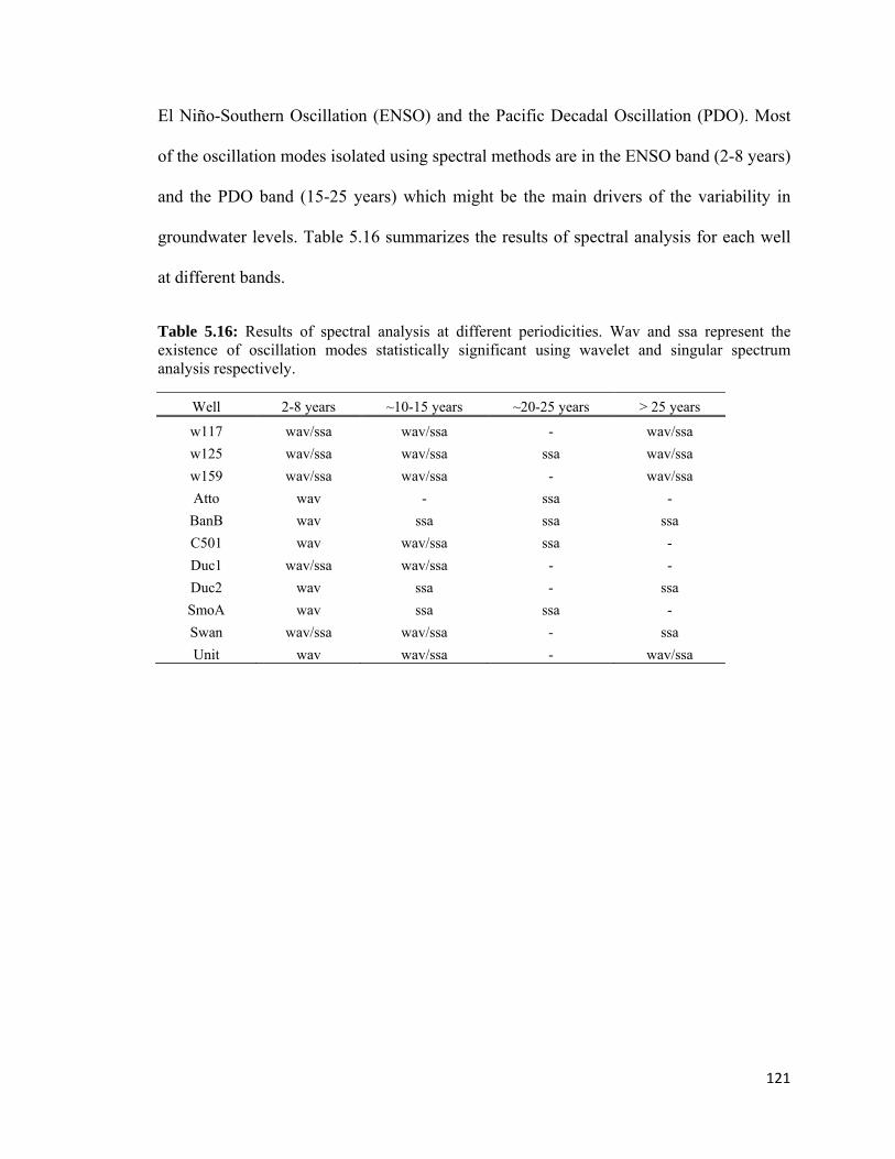
121

El Niño-Southern Oscillation (ENSO) and the Pacific Decadal Oscillation (PDO). Most

of the oscillation modes isolated using spectral methods are in the ENSO band (2-8 years)

and the PDO band (15-25 years) which might be the main drivers of the variability in

groundwater levels. Table 5.16 summarizes the results of spectral analysis for each well

at different bands.

Table 5.16: Results of spectral analysis at different periodicities. Wav and ssa represent the existence of oscillation modes statistically significant using wavelet and singular spectrum analysis respectively.

Well 2-8 years ~10-15 years ~20-25 years > 25 years

w117 wav/ssa wav/ssa - wav/ssa

w125 wav/ssa wav/ssa ssa wav/ssa

w159 wav/ssa wav/ssa - wav/ssa

Atto wav - ssa -

BanB wav ssa ssa ssa

C501 wav wav/ssa ssa -

Duc1 wav/ssa wav/ssa - -

Duc2 wav ssa - ssa

SmoA wav ssa ssa -

Swan wav/ssa wav/ssa - ssa

Unit wav wav/ssa - wav/ssa

122

6. CONCLUSIONS

6.1 Research findings

This study is the first to examine trends in groundwater levels and long term

variability in the Canadian Prairies and it has achieved each one of the objectives

described under heading 1.5.

The results indicate that 12 groundwater records present statistically significant

decreasing trends, 10 records do not register significant trends and 11 have increasing

trends. This study also found a spatial pattern in the distribution of trends through the

Prairies. Groundwater levels in north central areas are dominated by decreasing or no

trends, in contrast to groundwater levels in southern areas which are dominated by

increasing trends. This spatial pattern coincides with the spatial distribution in

evaporation trends identified in a previous study, where northern areas have increasing

trends and southern areas decreasing trends in evaporation and thus a negative correlation

with trends in groundwater levels This result ratifies the importance of evaporation in

aquifer recharge.

Strong linear relationships were found between groundwater levels and moisture-

sensitive tree-ring chronologies. This relationship made possible the use of multiple

linear regression techniques to reconstruct historical groundwater levels in Alberta and

Saskatchewan. These reconstructions expand groundwater records for more than 300

years in Alberta and more than 100 years in Saskatchewan. The tree-ring reconstructions

account for 40% to 81% of the instrumental variance in groundwater levels.

Longer periods of low groundwater levels than observed were identified in inferred

pre-instrumental water levels in Alberta and Saskatchewan. Also, these reconstructions

123

reveal the impact of historical climatic events and in particular droughts. For example the

1980s is the decade with the lowest water levels reconstructed at well 117 in more than

300 years. The Period centered on 1950 is the longest period with low water levels in the

320 year reconstruction at well 125. Mean water levels at well 159 have remained

relatively steady during the 144 year reconstruction, even though spectral methods

identified significant oscillation modes in the 2-8, 8-16, 16-32 year bands. The activity in

the 2-8 year band produces significant inter-annual variability but not always changes in

the mean. Activity in the same bands is also observed in groundwater levels at wells 117

and 125 and most of the activity in the 2-8 year band is significant after 1850.

The reconstruction models for Saskatchewan suggest that low water levels in the late

1990s early 2000s at wells Atto, Duc1, and SmoA are the lowest in 123, 93, and 123

years respectively. This is also the period with the lowest mean except at well Duc1

where the lowest period is centered on the 1950s. Groundwater at wells BanB, Duc2, and

Unit reached the lowest levels in the 1960s and this is the period with the lowest mean in

93, 127, and 127 years. Water levels at wells Swan reached the lowest level in the 1940s

and the period centered on 1910 registers the lowest mean.

Wavelet analysis identified most of the significant activity in Saskatchewan

groundwater levels in the 8-16 and 16-32 years bands. Activity in the 2-8 year band was

found in at some wells but it was not significant at all wells in Saskatchewan. Oscillation

modes in this band cause a greater inter-annual variability but it is not a driver of changes

in mean water levels. Oscillation modes in the 8-16 and 16-32 year bands account for

most of the variability in water levels in Saskatchewan. Common oscillation modes have

been identified at ~10 and ~15 years in the 8-16 year band, and ~20 and ~25 year.

124

Generally, changes in mean water levels are caused by the superposition of different

oscillation modes acting at the same time where different phases of these modes can

produce major impacts on groundwater levels.

6.2 Future research

As a result of this study, a groundwater data based has been generated for the

Canadian Prairies. This data base has been used for the first time to calculate trends in

groundwater levels and study long term climate variability. This study has answered

some questions about trends, natural variability, and impacts of historical droughts on

groundwater resources but also raises many more questions that lead to more research.

These topics for further research include seasonal trends in groundwater levels for a

common period, and the identification of spatial patterns as a function of evaporation and

precipitation. In addition, historical droughts have had different impacts on groundwater

levels at different wells which suggest that the quantification of the impacts climate

events such as droughts needs to be studied at aquifer level.

125

7. REFERENCES Abdul-Aziz, O.I. and D. H. Burn, 2006. Trends and variability in the hydrological regime

of the Mackenzie River basin.”Journal of Hydrology, 319(1-4), 282-294. Akinremi, O.O., and S. M. McGinn, 1999. Precipitation trends on the Canadian Prairies,

J. Clim. 12,2996–3003. Allen, D.M., D.C. Mackie, and M. Wei 2004. Groundwater and climate change: a

sensitivity analysis for the Grand Forks aquifer southern British Columbia, Canada. Hydrogeology Journal 12,270–290

Axelson J. 2007. Historical streamflow variability in the South Saskatchewan river basin

inferred from a network of tree-ring chronologies. MSc Thesis. University of Regina.

Bonsal, B., and E. Wheaton, 2005. Atmospheric Circulation Comparisons between the

2001 and 2002 and the 1961 and 1988 Canadian Prairie Droughts. Atmosphere-Ocean, 43(2), 163-172.

Burn, D. H., and M. A. Hag Elnur, M.A., 2002. Detection of hydrologic trend and

variability. Journal of Hydrology 255, 107–122. Burn, D.H., and N.M. Hesch, 2006. A comparison of trends in potential and pan

evaporation for the Canadian Prairies, Canadian Water Resources Journal, 31(3), 173-184.

Case, R.A., and G. M. MacDonald, 2003. Tree ring reconstruction of streamflow for three

Canadian Prairie Rivers. Journal of the American Water Resources Association 39,703-716.

Chen, Z., S. Grasby, and K. G. Osadetz, 2002. Predicting average annual groundwater

levels from climatic variables: An empirical model. Journal of Hydrology 260,102-117.

Cook, E. R., 1985. A time series analysis approach to tree-ring standardization. Ph.D.

Thesis, Univ. of Arizona, Tucson, USA. Cook, E. R., Kairiukstis, L.A., 1990. Methods of dendrochronology: applications in the

environmental sciences. Kluwer, Dordrecht. Coulibaly, P., and D.H. Burn, 2004. Wavelet analysis of the variability in Canadian

streamflows. Water Resources Research, 40, W03105, 1-14.

126

Dettinger, M.D., M. Ghil, C. M. Strong, W. Weibel, and P. Yiou, 1995. Software expedites singular-spectrum analysis of noisy time series, Eos Trans. AGU, 76(2), 12.

Ferguson G., and St. George, 2003. Historical and estimated ground water levels near

Winnipeg, Canada, and their sensitivity to climatic variability. Journal of the American Water Resources Association 39,1249-1259.

Fetter, C. W. 1994. Applied Hydrogeology. Macmillan, New York, 691 pp. Fleming, S.W., and E. J. Quilty, 2006. Aquifer responses to El Niño-Southern Oscillation, southwest British Columbia, Ground Water, 44(4), 595-599. Fritts, H.C., 1976. Tree rings and climate. Academic Press, London. Gan, T. Y., 1998. Hydroclimatic trends and possible climatic warming in the Canadian

Prairies, Water Resour. Res., 34,3009– 3015. Gan, T.Y., A. K. Gobena, and Q. Wang, 2007. Precipitation of southwestern of Canada:

Wavelet, scaling, multifractal analysis, and teleconnection to climate anomalies. Journal of Geophysical Research: 112, D10110

Ghil, M., Allen, R.M., Dettinger, M.D., Ide, K., Kondrashov, D., Mann, M.E., Robertson,

A., Saunders, A., Tian, Y., Varadi, F., Yiou, P., 2002. Advanced spectral methods for climatic time series. Rev. Geophys. 40 (1), 1.1–1.41.

Grinsted, A., J. C. Moore, and S. Jevrejeva, 2004. Application of cross wavelet transform

and wavelet coherence to geophysical time series, Nonlinear processes in geophysics, 11, 561-566.

Guiot, J. 1990. Tree-ring standardization and growth-trend estimation. In Cook, E.R. and

Kairiukstis, L.A. (Eds). Methods of Dendrochronology: Applications in the Environmental Sciences, Klumer Academic Publishers, Dordrecht:165-178.

Hirsch, R.M., and J.R. Slack, 1984. A nonparametric trend test for seasonal data with

serial dependence: Water Resources Research v. 20, p. 727–732. Holmes, R.L., 1983. Computer-assisted quality control in tree-ring dating and

measurements. Tree-Ring Bull. 43, 69–75. Daubechies, I. 1998. Recent results in wavelet applications, J. Electronic Imaging, 7 (4),

pp. 719-724. Intergovernmental Panel on Climate Change (IPCC) Working group I, 2007. Climate

Change 2007: The Physical science basis.

127

Jevrejeva, S., J.C. Moore, and A. Grinsted, 2003. Influence of the Arctic oscillation and El Niño-southern oscillation (ENSO) on ice conditions in the Baltic Sea: the wavelet approach. J. Geophys. Res. 108, 4677. doi:10.1029/2003JD003417.

Kendall, M.G., Rank Correlation Measures, Charles Griffin, London, 1975. Kharin V. V., F. W. Zwiers, 2000. Changes in the extremes in an ensemble of transient

climate simulations with a coupled Atmosphere-Ocean GCM. J. Climate, 13, 3760–3788

Lewis, J.E., 1989. Climatic change and its effects on water resources for Canada: a

review. Canadian Water Resources Journal 14,35–55. Loaiciga, H. A., L. Haston, and J. Michaelsen, J. 1993. Dendrohydrology and long-term

hydrologic phenomena. Reviews of Geophysics, 31(2): 151-171. Loáiciga H. A., Maidment, and J. B. Valdes. 2000. Climate-change impacts in a regional

karst aquifer, Texas, USA. Journal of Hydrology 227: 173–94. Loáiciga H. A. 2003. Sustainable groundwater exploitation. Int Geol Rev 44(12):1115–1121 Maathuis, H., and H. Thorleifson, 2000. Potential impact of climate change of prairie

groundwater supplies: review of current knowledge. Saskatchewan Research Council, Publication 11304-2E00, 43 p.

Mann, H.B., 1945. Nonparametric tests against trend. Econometrica 13, pp. 245–259. Meyers, S.D., B. G. Kelly, and J. J. O'Brien, 1993. An introduction to wavelet analysis in

oceanography and meteorology with application to the dispersion of Yanai waves. Monthly Weather Review 121, 2858–2866

Mitchell T. D. and P. D. Jones. 2005. An improved method of constructing a database of

monthly climate observations and associated high-resolution grids. International Journal of Climatology 25, 693-712.

Moore R.D, D.M. Allen and K. Stahl. 2007. Climate change and low flow: Influences of

groundwater and glaciers. Climate Change Action Fund, Natural resources Canada Final Report for Climate Change Action Fund Project A875

Nkemdirim, L., and L. Weber. 1999. Comparison between the droughts of the 1930s and

the 1980s in the southern prairies of Canada. Journal of Climate 12, no. 8, pt.1 (Aug): 2434-50.

128

Ostrom, C. W., Jr. 1990. Time Series Analysis, Regression Tehcniques, Second Edition: Quantative Applications in the Social Sciences, v. 07-009, Sage Publications, Newbury Park.

PFRA Hydrology Division, 1983. The Determination of Gross and Effective Drainage

Areas in the Prairie Provinces, Hydrology Report #104, Agriculture Canada, PFRA Engineering Branch, Regina, Saskatchewan, 22 pp.

Rodionov, S.N., 2004. A sequential algorithm for testing climate regime shifts. Geophys.

Res. Lett., 31, L09204, doi:10.1029/2004GL019448. Sauchyn, D. and S. Kulshreshtha et al. (2008) “Prairies” in From Impacts to Adaptation:

Canada in a Changing Climate 2007, edited by D. Lemmen et al., Government of Canada, Ottawa.

Schindler, D.W., Bayley, S., Parker, B., Beaty, K., Cruikshank, D., Fee, E., Schindler, E.

and Stainton, M., 1996. The effects of climatic warming on the properties of boreal lakes and streams at the experimental lake area, northwestern Ontario. Limnology and Oceanography 41 5, pp. 1004–1017

St. George, S. and E. Nielsen, 2002. Hydroclimatic Change in Southern Manitoba Since

A.D. 1409 Inferred From Tree Rings. Qauternary Research 58(2),103-111. Stokes, M.A., Smiley, T.L., 1968. An introduction to tree-ring dating. Univ. of Chicago

Press, Chicago, IL. Torrence, C., and G. P. Compo, 1998. A practical guide towavelet analysis. Bull. Am.

Meteorol. Soc. 79, 61–78. van der Kamp G. and H. Maathuis, 1991. Annual fluctuations of groundwater levels due

to loading by surface moisture, Journal of Hydrology 127 (1991), pp. 137–152. Vautard, R., and M. Ghil, 1989: Singular spectrum analysis in nonlinear dynamics with

applications to paleoclimatic time series. Physica D, 35, 395-424 Vautard, R., P. Yiou, and M. Ghil, 1992: Singular Spectrum Analysis: A toolkit for short,

noisy, chaotic time series. Physica D, volume 38, pp. 74-95 Von Storch, H. 1995. Misuses of statistical analysis in climate research. In: Analysis of

Climate Variability: Applications of Statistical Techniques (ed. by H. von Storch & A. Navarra), 11–26. Springer-Verlag, Berlin, Germany

Watson, E. and B. H. Luckman, 2001. Dendroclimatic reconstruction of precipitation for

sites in the southern Canadian Rockies. The Holocene 11,203-213. Wheaton, E., S. Kulshreshtha, and V. Wittrock, V. eds. 2005 Canadian Droughts of 2001

and 2002: Climatology, Impacts and Adaptations (Saskatoon, SK: Saskatchewan

129

Research Council). Technical report prepared for Agriculture and Agri- Food Canada. SRC Publication No. 11602–1E03, 13

Woldeamlak S. T, , O. Batelaan and F. De Smedt 2007. Effects of climate change on the

groundwater system in the Grote-Nete catchment, Belgium . Hydrogeology Journal 15: 891–901

Woodhouse, C. A., 2001. A tree-Ring reconstruction of streamflow for the Colorado

Front Ranges. Journal of the American Water Resources Association (JAWRA) 37,561-569.

Yue et al., 2002 S. Yue, P. Pilon, B. Phinney and G. Cavadias, The influence of

autocorrelation on the ability to detect trend in hydrological series, Hydrological Processes 16 (2002), pp. 1807–1829.

130

APPENDIX

Table A1: Coefficients of autocorrelation functions (ACF)

Well ACF(1) ACF(2) ACF(3) ACF(4) ACF(5)

w102 0.925* 0.792* 0.645 0.458 0.256

w104 0.850* 0.688* 0.530 0.386 0.240

w106 0.825* 0.540 0.258 ‐0.013 ‐0.223

w108 0.677* 0.230 ‐0.196 ‐0.459 ‐0.452

w112 0.825* 0.624 0.488 0.297 0.135

w114 0.764* 0.266 ‐0.221 ‐0.541 ‐0.619

w117 0.681* 0.390 0.273 0.192 0.100

w125 0.597* 0.107 ‐0.158 ‐0.309 ‐0.231

w147 0.330* ‐0.119 0.071 0.304 0.061

w159 0.649* 0.059 ‐0.381 ‐0.575 ‐0.474

w176 0.637* 0.092 ‐0.322 ‐0.494 ‐0.418

w192 0.869* 0.626 0.323 0.032 ‐0.220

w193 0.911* 0.763 0.561 0.339 0.104

w212 0.766* 0.575 0.354 0.131 0.017

w228 0.814* 0.536 0.293 0.024 ‐0.177

w229 0.632* 0.271 0.065 ‐0.218

w252 0.483* ‐0.132 ‐0.239 ‐0.289 ‐0.445

w260 0.869* 0.710* 0.567 0.424 0.270

w270 0.804* 0.498 0.195 ‐0.049 ‐0.150

Atto 0.921* 0.821* 0.725* 0.641 0.558

B059 0.896* 0.783* 0.693* 0.595 0.536

BanA 0.931* 0.785* 0.594* 0.383 0.182

BanB 0.914* 0.765* 0.579 0.374 0.176

C500 0.857* 0.698* 0.526 0.375 0.265

C501 0.813* 0.524 0.290 0.121 0.066

Duc1 0.749* 0.373 0.167 0.125 0.094

Duc2 0.851* 0.634* 0.419 0.269 0.173

Lila 0.936* 0.850* 0.765* 0.694 0.619

Rice 0.925* 0.834* 0.748* 0.656 0.572

Si13 0.806* 0.611* 0.470 0.337 0.274

SmoA 0.882* 0.725* 0.581 0.450 0.334

Swan 0.888* 0.768* 0.617 0.496 0.397

Tyne 0.889* 0.777* 0.699* 0.628 0.568

Unit 0.891* 0.767* 0.636 0.520 0.415

Verl 0.928* 0.860* 0.804* 0.724 0.630

Ln001 0.504* 0.081 ‐0.021 0.051 0.073

Ob005 0.867* 0.718* 0.604 0.486 0.331

Oe001 0.870* 0.724* 0.624 0.467 0.278

Og003 0.696* 0.470* 0.308 0.261 0.113

groundwater in the canadian prairies: trends and … · groundwater could be an increasingly...

Documents