groundwater potential mapping using a novel data-mining
TRANSCRIPT

PAPER
Groundwater potential mapping using a novel data-miningensemble model
Mojtaba Dolat Kordestani1 & Seyed Amir Naghibi2 & Hossein Hashemi2 & Kourosh Ahmadi3 & Bahareh Kalantar4 &
Biswajeet Pradhan5,6
Received: 12 January 2018 /Accepted: 5 August 2018 /Published online: 1 September 2018# The Author(s) 2018
AbstractFreshwater scarcity is an ever-increasing problem throughout the arid and semi-arid countries, and it often results inpoverty. Thus, it is necessary to enhance understanding of freshwater resources availability, particularly for groundwater,and to be able to implement functional water resources plans. This study introduces a novel statistical approach com-bined with a data-mining ensemble model, through implementing evidential belief function and boosted regression tree(EBF-BRT) algorithms for groundwater potential mapping of the Lordegan aquifer in central Iran. To do so, springlocations are determined and partitioned into two groups for training and validating the individual and ensemblemethods. In the next step, 12 groundwater-conditioning factors (GCFs), including topographical and hydrogeologicalfactors, are prepared for the modeling process. The mentioned factors are employed in the application of the EBF model.Then, the EBF values of the GCFs are implemented as input to the BRT algorithm. The results of the modeling processare plotted to produce spring (groundwater) potential maps. To verify the results, the receiver operating characteristics(ROC) test is applied to the model’s output. The findings of the test indicated that the areas under the ROC curves are 75and 82% for the EBF and EBF-BRT models, respectively. Therefore, it can be inferred that the combination of the twotechniques could increase the efficacy of these methods in groundwater potential mapping.
Keywords Geographic information system (GIS) . Groundwater management . Data mining . Iran
Introduction
Groundwater could be regarded as the water in the saturatedparts of the Earth that fills the pore section of geologic forma-tions and soil beneath the water table (Freeze and Cherry1979). Groundwater has broad advantages over surface wateras a resource, including its capability to be utilized whenneeded, and it is less vulnerable to catastrophic incidents(Naghibi and Pourghasemi 2015). Furthermore, groundwatercontributes the most in meeting freshwater demand in arid andsemi-arid areas such as the Middle East (Chezgi et al. 2015).Groundwater potential mapping is one of the well-studiedsubjects in the literature and has attracted many researchersover the years.
Many researchers have used statistical and data miningalgorithms to map groundwater potential. Some of them haveused spring locations as groundwater resource indicators,while others used qanat and well locations. According to theliterature, the frequency ratio (Oh et al. 2011; Pourtaghi andPourghasemi 2014; Naghibi et al. 2015), weights-of-evidence
* Seyed Amir [email protected]; [email protected]
1 University of Hormozgan, Jiroft University Scholarship, Departmentof Combat Desertification, Faculty of Rangeland and WatershedManagement, Jiroft University, Jiroft, Iran
2 Center for Middle Eastern Studies & Department ofWater ResourcesEngineering, Lund University, Lund, Sweden
3 Department of Forestry, College of Natural Resources, TarbiatModares University, Noor, Mazandaran, Iran
4 RIKEN Center for Advanced Intelligence Project, Goal-OrientedTechnology Research Group, Disaster Resilience Science Team,Tokyo 103-0027, Japan
5 Centre for AdvancedModelling and Geospatial Information Systems(CAMGIS), Faculty of Engineering and IT, University ofTechnology Sydney, Sydney, NSW 2007, Australia
6 Department of Energy and Mineral Resources Engineering,Choongmu-gwan, Sejong University, 209 Neungdong-ro,Gwangjin-gu, Seoul 05006, Republic of Korea
Hydrogeology Journal (2019) 27:211–224https://doi.org/10.1007/s10040-018-1848-5

(Ozdemir 2011a; Corsini et al. 2009; Razandi et al. 2015;Tahmassebipoor et al. 2016), and index of entropy (Naghibiet al. 2015) are among the most popular methods used by thescholars. Moreover, other data mining methods such as clas-sification and regression tree, random forest, and boosted re-gression tree (BRT) are widely used to assess the potential ofgroundwater (e.g. Naghibi and Pourghasemi 2015; Naghibi etal. 2016; Zabihi et al. 2016; Rahmati et al. 2016; Mousavi etal. 2017; Golkarian et al. 2018). Although data mining tech-niques have proved to be reliable in working with nonlinearand complex data (Naghibi et al. 2016), one of the drawbacksis overfitting, which impacts the models’ estimation qualityand prediction validity. In two recent papers, by Naghibi andMoradi Dashtpagerdi (2016) and Naghibi et al. (2018), vari-ous data mining algorithms, including random forest, BRT,support vector machine, artificial neural network, quadraticdiscriminant analysis, linear discriminant analysis, flexiblediscriminant analysis, penalized discriminant analysis, k-nearest neighbors, and multivariate adaptive regressionsplines, were employed for groundwater assessment takinginto account spring and qanat locations. Other techniques in-clude the evidential belief function (EBF) method to map thepotentiality of groundwater (Nampak et al. 2014; Rahmati andMelesse 2016). Nampak et al. (2014) used EBF to mapgroundwater potential and compared its performance with alogistic regression model; the results indicated the superiorperformance of the EBF model. In another research project,Naghibi and Pourghasemi (2015) examined the efficacy of theEBF model and compared the results with classification andregression tree, random forest, BRT, and generalized linearmodel. Their findings also yielded an acceptable performanceof the EBF model.
The aforementioned studies mostly used single models inthe groundwater-related research; however, the ensemblemodels have been used in other fields of study including land-slides (Lee et al. 2012; Umar et al. 2014) and flood suscepti-bility modelling (Tehrany et al. 2013, 2014). Very recently,Naghibi et al. (2017b) introduced a novel ensemble model,which was constructed based on four data mining modelsand the frequency ratio in a groundwater-related study. Thefindings of their research indicated that the produced ensem-ble model showed a better performance than a single applica-tion of the models. Similarly, Pourghasemi and Kerle (2016)combined EBF and random forest models to achieve bettermodel performance and their results indicated a higher effica-cy of the ensemble method.
Boosted regression tree as a data mining technique wasselected for this purpose as it has the capability for featureselection (Naghibi et al. 2016) as well as implementing sto-chastic gradient boosting to diminish variance and bias(Abeare 2009). The BRT model also defines the importanceof the impacting factors in the modelling procedure.Considering the aforementioned strong features of the BRT
model, this model was chosen to be combined with the EBFmodel to improve its prediction accuracy. In this research, theproposed ensemble method (EBF-BRT) improves on theweak points of each method and combines their advantagesby analyzing the relationships of groundwater with each inde-pendent layer and with each class of independent layers; fur-thermore, groundwater-related independent variables can beassessed. Since this combined approach is almost new ingroundwater potential assessment, through this research itsefficiency and capability can be examined. This research aimsto improve the performance of statistical techniques throughthe extension of a data-mining ensemble model in groundwa-ter potential mapping. Thus, the aims of this study are: (1)evaluating the performance of the EBF-BRTmodel in ground-water potentiality assessment, (2) ranking the importance ofgroundwater-conditioning factors (GCFs) and the relationshipbetween groundwater potential and the GCFs, and (3) provid-ing spatial information and guidance to support decision-making processes concerning groundwater management inthe Lordegan aquifer in central Iran.
Materials and methods
A spring can be defined as a feature by which groundwaterflows from an aquifer to the land surface. Based on the phys-iographical and hydrological characteristics of the study area,this study assumes that the natural spring occurrences andtheir discharge rates can be related to the potential of ground-water resources in the studied basin. To quantify this relation-ship, a groundwater potential map (GPM) is proposed as a toolfor providing spatial information and for determining the re-lationship between the spring occurrence and effective factors,here called ‘conditioning factors’.
For modelling of groundwater potential, two datasets wereprepared, including a springs location inventory and theGCFs. Using the mentioned datasets, the EBF model wasimplemented, and the resultant GPM was plotted usingArcGIS 10.4. In the next step, EBF values were extractedand then used as an input to the BRTmodel, and the ensembleEBF-BRT model was trained. Finally, by implementing a re-ceiver operating characteristics (ROC) plot, the efficacy of theEBF and EBF-BRT methods were validated. Figure 1 showsthe methodology flowchart implemented in this research.
Study area and preparation of the conditioningfactors
Study area
The Lordegan Basin covers the areas between 31°19′09″ and31°38′06″ north latitudes and 50°28′02″ and 51°13′13″ eastlongitudes, and is located in Chaharmahal-e-Bakhtiari
212 Hydrogeol J (2019) 27:211–224

Province, Iran. Lordegan Basin covers an area of 1,486 km2.The topographic elevation in Lordegan Basin ranges between850 and 3,640 m above mean sea level (amsl) with a meanelevation of 2,044 m amsl. The lithology of the LordeganBasin is mainly composed of sedimentary and tertiary rocksand Quaternary deposits, and about 33.3% of its area is clas-sified under group 5, including low-level piedmont fan andvalley terraces deposits (GSI 1997; Table 1). The dominantland use is rangeland, which covers approximately 44% of thebasin floor. Other types of land use encompass forest, agricul-ture, orchard, and residential area. Spring occurrence is notlimited to the plain areas and it can be seen on different slopesand elevations; hence, the study was carried out at the basinscale.
Data preparation
In this study, a spring inventory dataset including 94 springs(in 2014) was prepared based on the field surveys (Fig. 2). Thedataset was then split into two subsets for training (70% of thedataset: 66 springs) and validating (30% of the dataset: 28springs) the models (Pourghasemi and Beheshtirad 2015). Itshould be noted that the division of the spring dataset into twosubsets was conducted on the basis of a random algorithm inArcGIS 10.4.
Based on the literature (Ozdemir 2011a, b) and availabilityof data, 12 GCFs were selected for the modelling process. TheGCFs are composed of eight topographical factors, two river-
related factors, and two physical factors including land useand lithology. It should be noted that as the EBF works withclassified factors, the GCFs were classified based on the liter-ature (Ozdemir 2011a, b; Naghibi et al. 2018).
In the first step, a 20-m resolution digital elevation model(DEM) of the studied basin was derived from a 1:50,000-scaletopographic map. The slope angle derived from the DEMwassplit into four ranges of 0–5, 5–15, 15–30, and >30° (Fig. 3a).Slope aspect was also derived from DEM data and then clas-sified into nine classes (Fig. 3b). Elevation is another impor-tant GCF (Ozdemir 2011a, b) that was employed in this in-vestigation (Fig. 3c). The elevation of the studied basin waspartitioned into five equal classes.
Plan curvature is a topographical-based variable, whichshows the direction of flow (Ozdemir 2011a; Fig. 3d).Profile curvature clarifies at which rate the slope changes inthe maximum slope direction (Ozdemir 2011b; Fig. 3e). Slopelength (LS) is considered as a mixture of the two variables ofslope steepness and slope length (Naghibi et al. 2016) and iscalculated as follows (Moore et al. 1991; Fig. 3f):
LS ¼ As
22:13
� �0:6 sinα0:0896
� �1:3
ð1Þ
where, As depicts the specific watershed area and α is theestimated slope gradient (degree).
The stream power index (SPI) could be implemented toshow potential flow erosion at a specific location of the basin(Moore and Burch 1986; Fig. 3g). Further, the topographic
Fig. 1 Flowchart of the methodology implemented in this study
Hydrogeol J (2019) 27:211–224 213

wetness index (TWI) was taken into account in this investiga-tion. TWI denotes the spatial changes of soil moisture (Mooreand Burch 1986; Fig. 3h).
Distance from rivers and river density are two crucial GCFsthat affect the groundwater potentiality (Naghibi et al. 2015).These two layers were calculated in ArcGIS 10.4 usingEuclidean distance and line density functions. Concerningthe distance from rivers, 100 m-intervals were chosen, andthe distances were then classified into five groups (Fig. 3i).A rivers density map was partitioned into four categories by anatural break classification method (Fig. 3j).
A land use map was produced by implementing Landsat 8/Enhance Thematic Mapper Plus (ETM+) images for the year2015 based on a likelihood algorithm. The land use mapcontained five different land use classes: orchard, residentialarea, rangeland, agriculture, and forest (Fig. 3k).
Geology is composed of three GCFs including lithologicalclasses, and fault-related factors such as distance and densitymaps (Naghibi et al. 2016). After investigating the fault layerof the studied region, it was found that only a tiny portion ofthe studied region is affected by faults; therefore, fault-relatedfactors were not considered in the current research. Based on a
Table 1 Lithology characteristicsof Lordegan Basin, Iran Lithology group Lithology characteristics
1 Anhydrite, salt, grey and red marl, alternating with anhydrite, argillaceous limestoneand limestone
2 Blue and purple shale and marl inter-bedded with the argillaceous limestone
3 Bluish grey marl and shale with subordinate thin-bedded argillaceous-limestone
4 Brown to grey, calcareous, feature-forming sandstone and low-weathering,gypsum-veined, red marl and siltstone
5 Low-level piedmont fan and valley terrace deposits
6 Low-weathering grey marls alternating with bands of more resistant shelly limestone
7 Pale red marl, marlstone, limestone, gypsum and dolomite
8 Cream to brown color, weathering, feature-forming, well-jointed limestone withintercalations of shale
9 Dark red, medium-grained arkosic to subarkosic sandstone and micaceous siltstone
10 Limestone, dolomite, dolomitic limestone and thick layers of anhydrite in alternationwith dolomite in middle part
11 Massive, shelly, cliff-forming partly anhydrite limestone
12 Undivided Bangestan group, mainly limestone and shale, Albian era
13 Undivided Eocene rock
Fig. 2 Locations of the study area in Iran, and the training and validation springs
214 Hydrogeol J (2019) 27:211–224

Fig. 3 The groundwater-conditioning factors (GCFs) considered in thisstudy: a slope angle, b slope aspect, c elevation, d plan curvature, e profilecurvature, f slope length, g stream power index (SPI), h topographic
wetness index (TWI), i distance from rivers, j rivers density, k land use,and l lithology
Hydrogeol J (2019) 27:211–224 215

Fig. 3 (continued)
216 Hydrogeol J (2019) 27:211–224

1:100,000-scale geological map, the geological units werepartitioned into thirteen units including groups 1–13 (Table1; Fig. 3l).
Modelling process
In this section, a description of the models is presented andthen the process of applying a novel data-mining model (EBF-BRT) is explained.
Evidential belief function (EBF) model
The EBFmodel is developed based on the Dempster–Shaferapproach of evidence (Dempster 1967; Shafer 1976), whichincludes uncertainty (Unc), belief (Bel), plausibility (Pls),and disbelief (Dis) that change from 0 to 1 (Carranza andHale 2003). This model has a relative flexibility and is ableto work with uncertain conditions (Nampak et al. 2014). Inthe Dempster–Shafer theory, Bel and Pls define the lowerand upper probabilities of the generalized Bayesian theo-rem, respectively (Nampak et al. 2014). Therefore, it canbe inferred that Bel is greater than or equal to Pls. Unc couldbe calculated by differentiating Pls and Bel values (Naghibiand Pourghasemi 2015). Based on the evidential data, dis-belief depicts the belief in the false proposition. For calcu-lating the Bel value, first, a frame of discernment could becalculated (Dempster 1967; Shafer 1976; Pourghasemi andBeheshtirad 2015):
m : 2Θ ¼ ϕ; TP; TP;Θn o
with Θ ¼ TP; TP
n oð2Þ
where TP shows the pixels that include springs, TP showsthe pixels that do not include springs, and ϕ represents theempty set.
From Eq. (1), the Bel function could be computed as fol-lows (Park 2011; Pourghasemi and Beheshtirad 2015):
λ TPð ÞAij
h i¼
N S∩Aijð ÞN Sð Þ
" #= N Aij−N S∩Aijð Þ
� �� �= N Pð Þ−N Sð Þ� �h i
ð3Þ
Bel ¼λ SPð ÞAij
∑λ SPð ÞAij
" #ð4Þ
where N S∩Aijð Þ denotes the density of spring pixels incidencein Aij,N(S) denotes the total density of all springs in the studiedbasin, N Aijð Þ represents the density of pixels in Aij, and N(P) isthe density of pixels in the whole studied basin. More descrip-tions and information about EBF algorithm could be found inCarranza and Hale (2003).
The novel data-mining ensemble model
The BRT is a data-mining/machine-learning approach, whichcomprises of both decision trees and boosting techniques andcould be employed for both regression and classification is-sues (Youssef et al. 2015). It aims to increase the efficacy aswell as prediction capability of single methods by combiningseveral fittedmodels (Naghibi et al. 2016). Boosting is appliedin order to combine the results of the decision trees, which issimilar to model averaging. There are some parameters thatrequire optimizing in this model such as a number of trees,shrinkage (or learning rate), and interaction depth. Shrinkageor learning rate defines the importance of trees in the builtmodel (Naghibi et al. 2016). Interaction depth or complexitydetermines the number of nodes in trees.
The BRT model can be explained as follows (Elith et al.2008; Naghibi et al. 2016):
Starting weights to be equal to fi = 1/n.For m = 1 to iteration classifier Cm):
1. Run classifier Cm to the weighted data2. Calculate misclassification rate rm3. Consider the classifier weight αmlog
1−rmð Þrm
� �4. Recalculate weights wi =wi exp[αmI(yi ≠Cm)]
Finally, the majority vote can be obtained by:
sign ¼ ∑Mm−1αmCm Xð Þ� �
It is noted that the best set of parameters in BRT wereselected by using the accuracy index and Cohen’s kappa in-dex, which can be calculated as follows:
Accuracy ¼ TPþ TN
TPþ TNþ FPþ FNð5Þ
Kappa ¼ Pobs−Pexp
1−Pobsð6Þ
Pobs ¼ TPþ TN=n ð7Þ
Pexp ¼ TPþ FNð Þ TPþ FPð Þ þ FPþ TNð Þ FNþ TNð Þ=ffiffiffiffiN
p ð8Þ
where n is the ratio of cells that are correctly categorized, andN shows the number of total training cells, while TP, FP, TN,and FN represent true positive, false positive, true negative,and false negative, respectively (Naghibi and MoradiDashtpagerdi 2016).
To apply a novel data-mining ensemble model, first, theEBF model was applied and belief values were assigned todifferent classes of the GCFs. Then, new maps of each factorwere produced by the lookup function in ArcGIS 10.4. A newdataset was provided for training of the data-mining model(i.e. BRT). In this dataset, 1 was assigned to the spring and 0was assigned to nonspring locations. It is noted that the
Hydrogeol J (2019) 27:211–224 217

nonspring locations were randomly defined using ArcGIS10.4. Using the new training dataset and new GCFs layerswith Bel values, the BRT model was conducted using Ropen-source software via the gbm package (Ridgeway2006). The BRT model was run using a 10-fold cross-valida-tion, deemed to be a sufficient number of runs for optimizationof the assigned parameters. It needs to be clarified that theGPMs produced by the EBF and BBF-BRT methods are clas-sified into four classes—low, moderate, high, and very high—by the natural break classification method (Naghibi et al.2018).
Results and discussion
GPM production by evidential belief function
The results of the EBF model are presented in Table 2 wherethe values of the Bel, Dis, and Unc are reported. As mentionedin the methodology section, a class with high Bel value has ahigh potential for the occurrence of the event, which in thiscase is the existence of a spring (Nampak et al. 2014;Pourghasemi and Beheshtirad 2015). Based on the results, itcan be observed that there is an inverse relationship betweenslope angle and the Bel value, which means that the ground-water potential decreases with the increase in slope angle.Regarding the results of slope aspect, flat and north-east clas-ses show the highest Bel values. In contrast, south-east andsouth-west classes have Bel value of zero, which indicatestheir low potential of spring incidence. This finding can berelated to the less sunshine duration over the north slope as-pects in the northern hemisphere. In the case of elevation, theresults indicated that an inverse relationship exists betweenGCF and spring incidence. At lower elevations, water hasconcentrated near the rivers and, therefore, the wetness indexis higher in these areas which can result in the higher potentialof groundwater. The flat characteristic of the plan curvaturehad the highest Bel value (Bel = 0.54). The highest Bel valuewas observed in the (−0.001)–(0.001) category of the profilecurvature. An inverse relationship was observed between theslope length and spring incidence. In the case of SPI, theresults indicated that <200 and 400–600 categories have thehighest Bel value of 0.34 and 0.24, respectively. The findingsof TWI signified a direct relationship between TWI and springincidence. Regarding the distance from rivers, an inverse re-lationship between the distance from river and the spring oc-currence was observed. Regarding river density, the 0.86–1.46class has the highest Bel value of 0.40 followed by >1.46,0.31–0.86, and <0.31 classes. The modeling results with re-spect to land use showed that agriculture has the highest Belvalue, followed by forest and rangeland. Regarding lithology,the highest values of Bel were observed for group 2 and group10 with values of 0.22 and 0.17, respectively.
Overall, these findings signified that a direct relationshipexists between spring incidence and TWI factor. In contrast,an inverse relationship was observed between thegroundwater potentiality and three GCFs includingelevation, slope length, and distance from rivers. Naghibiand Pourghasemi (2015) obtained the same relationship be-tween elevation, TWI, and distance from rivers and springoccurrence. However, in some other factors such as LS, thefindings of this study differ from the findings of Naghibi andPourghasemi (2015). These differences can be due to the dif-ferent properties of the studied regions (i.e. topographical andhydrological characteristics). Furthermore, the results of theEBF-BRT model revealed that the distance from rivers, lithol-ogy, river density, and plan curvature had the highest impor-tance in the groundwater potential mapping of the studiedbasin.
The GPM produced by the EBF model in the current studyis presented in Fig. 4a and Table 3. It should be noted that thefinal EBF map was obtained by summing all the Bel values.Based on the findings, the value of GPM in this model rangesfrom 0.88 to 5.29. Low, moderate, high, and very high poten-tial categories composed 34, 28, 20, and 18% of the studiedbasin, respectively.
GPM production by the novel data-mining ensemblemodel
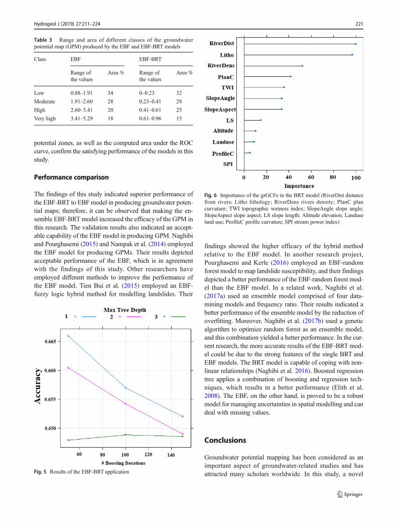
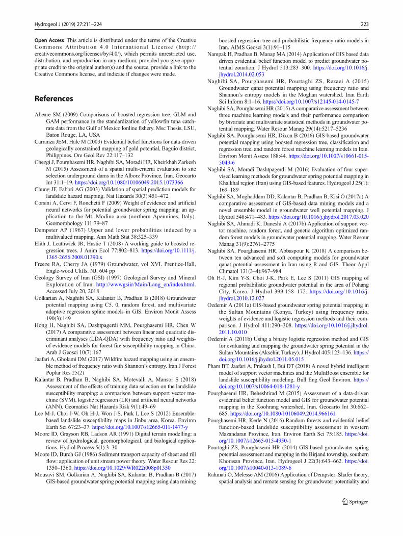
The findings of the application of BRT algorithm are present-ed in Fig. 5. The final BRT model was applied with the min-imum terminal node size of 10, shrinkage value of 0.1, 50number of trees, and interaction depth of 1 (accuracy index =0.66 and Cohen’s Kappa index = 0.33). The contribution ofthe GCFs to the modelling process is presented in Fig. 6. Theresults indicated that the distance from rivers, lithology, riverdensity, and plan curvature have the highest contribution togroundwater potential estimated by the EBF-BRTmodel (Fig.6). The land use and profile curvature showed the lowest con-tribution and SPI showed no effect on groundwater potential.The GPM obtained from the EBF-BRTmethod is presented inFig. 4b and Table 3. The GPM produced by the EBF-BRTmodel resulted in low, moderate, high, and very high potentialcategories, which composed 32, 28, 25, and 15% of the stud-ied basin, respectively.
Validation and verification of the GPMs
This section includes two steps: (1) validation of the mapsusing the validation dataset and ROC curve and (2) verifyingthe results by taking the observed spring discharges into ac-count. Chung and Fabbri (2003) stated that the validation isregarded as a very necessary stage in the modeling procedure.To do so, the ROC curve was implemented to define the ac-curacy of the GPMs produced by the EBF and EBF-BRT
218 Hydrogeol J (2019) 27:211–224

Table 2 Spatial relationshipbetween GCFs and springs usingthe EBF model
Factor Class % of pixelsin domain
No. ofsprings
Bel Dis Unc
Slope angle (degree) 0–5 29.46 38 0.54 0.15 0.31
5–15 22.58 20 0.37 0.23 0.41
15–30 35.25 8 0.09 0.34 0.57
>30 12.71 0 0.00 0.29 0.71
Slope aspect Flat 8.70 10 0.22 0.19 0.59
North 13.59 8 0.11 0.21 0.68
Northeast 14.69 13 0.17 0.19 0.64
East 8.65 4 0.09 0.21 0.70
Southeast 8.66 6 0.00 0.00 1.00
South 10.47 4 0.07 0.21 0.72
Southwest 13.60 10 0.00 0.00 1.00
West 11.17 8 0.14 0.00 0.86
Northwest 10.47 3 0.06 0.00 0.94
Elevation (m) <1400 1.63 4 0.61 0.24 0.15
1400–1900 40.15 36 0.22 0.19 0.58
1900–2500 45.22 25 0.14 0.29 0.57
2500–3000 9.22 1 0.03 0.28 0.70
>3000 3.79 0 0.00 0.00 1.00
Plan curvature (100/m) Concave 29.54 16 0.28 0.36 0.36
Flat 37.60 39 0.54 0.22 0.24
Convex 32.86 11 0.18 0.42 0.41
Profile curvature (100/m) < (−0.001) 35.30 23 0.33 0.34 0.33
(−0.001)-(0.001) 32.79 30 0.46 0.27 0.27
> (0.001) 31.91 13 0.21 0.39 0.40
Slope length (m) <20 38.46 40 0.41 0.16 0.43
20–40 16.73 12 0.29 0.25 0.47
40–60 14.23 8 0.22 0.26 0.52
>60 30.58 6 0.08 0.33 0.59
Stream power index <200 30.62 27 0.34 0.21 0.45
200–400 12.96 7 0.21 0.26 0.54
400–600 9.55 6 0.24 0.25 0.51
>600 46.87 26 0.21 0.28 0.50
Topographic wetness index <8 19.44 2 0.05 0.39 0.56
8–12 56.23 32 0.29 0.38 0.33
>12 24.33 32 0.66 0.22 0.12
Distance from rivers (m) <100 4.69 27 0.71 0.17 0.12
100–200 4.15 5 0.15 0.27 0.58
200–300 4.10 2 0.06 0.28 0.66
300–400 4.03 1 0.03 0.28 0.69
>400 83.04 31 0.00 0.00 1.00
River density (km/km2) <0.31 60.74 18 0.08 0.42 0.50
0.31–0.86 11.82 8 0.18 0.23 0.60
0.86–1.46 21.94 33 0.40 0.14 0.45
>1.46 5.50 7 0.34 0.21 0.45
Land use Agriculture 24.58 33 0.61 0.16 0.23
Forest 30.83 11 0.16 0.30 0.54
Orchard 0.04 0 0.00 0.25 0.75
Rangeland 43.99 22 0.23 0.29 0.48
Residential area 0.57 0 0.00 0.00 1.00
Hydrogeol J (2019) 27:211–224 219

models. The GPMs were verified employing training and val-idation datasets. The area under the curve of ROC varies be-tween 0.5 and 1 (Sangchini et al. 2016; Hong et al. 2017;Kalantar et al. 2018). A larger area under the curve of ROCdenotes higher efficacy of the models in spatial modeling(Jaafari and Gholami 2017; Pham et al. 2018) such as ground-water potential mapping. Figure 7 presents the prediction per-formance of the produced GPMs by EBF and EBF-BRTmodels implementing the ROC curve. Accordingly, the areaunder the curve of ROC for the validation dataset was definedas 75.5 and 82.1% for EBF and EBF-BRTmodels, respective-ly. Further, the area under the ROC curve for the trainingdataset was calculated as 77.2 and 83% for EBF and EBF-BRT, respectively. It was assumed that the values of more than
70% indicate an acceptable performance of the model(Naghibi et al. 2016).
To verify the resulting groundwater potential map of thebasin, the spring discharge record was used. For this, the ob-served discharge values higher than the median discharge,0.75 L/s, were selected for the models’ verification.Distribution of the selected springs in different potential zonesproduced by EBF and EBF-BRT is presented in Table 4. Ascan be seen in the table that, among 47 high-discharge springs,15 and 16 springs were located in the very high potential zoneproduced by EBF and EBF-BRT, respectively. According tothe modeling results, very few springs with high dischargewere located in the low potential zone (Table 4). The distribu-tion of the high-discharge springs in the identified groundwater
Fig. 4 Groundwater potential map produced by the a EBF and b EBF-BRT models
Table 2 (continued)Factor Class % of pixels
in domainNo. ofsprings
Bel Dis Unc
Lithology Group 1 3.25 4 0.16 0.07 0.76
Group 2 4.22 7 0.22 0.07 0.71
Group 3 0.22 0 0.00 0.08 0.92
Group 4 4.44 5 0.15 0.07 0.78
Group 5 33.32 26 0.10 0.07 0.82
Group 6 8.23 2 0.03 0.08 0.89
Group 7 1.53 0 0.00 0.08 0.92
Group 8 28.52 17 0.08 0.08 0.84
Group 9 2.39 1 0.06 0.08 0.87
Group 10 1.60 2 0.17 0.08 0.76
Group 11 0.02 0 0.00 0.08 0.92
Group 12 1.40 0 0.00 0.08 0.92
Group 13 10.86 2 0.03 0.08 0.89
Bel belief, Dis disbelief, Unc uncertainty
220 Hydrogeol J (2019) 27:211–224
potential zones, as well as the computed area under the ROCcurve, confirm the satisfying performance of the models in thisstudy.
Performance comparison
The findings of this study indicated superior performance ofthe EBF-BRT to EBF model in producing groundwater poten-tial maps; therefore, it can be observed that making the en-semble EBF-BRT model increased the efficacy of the GPM inthis research. The validation results also indicated an accept-able capability of the EBF model in producing GPM. Naghibiand Pourghasemi (2015) and Nampak et al. (2014) employedthe EBF model for producing GPMs. Their results depictedacceptable performance of the EBF, which is in agreementwith the findings of this study. Other researchers haveemployed different methods to improve the performance ofthe EBF model. Tien Bui et al. (2015) employed an EBF-fuzzy logic hybrid method for modelling landslides. Their
findings showed the higher efficacy of the hybrid methodrelative to the EBF model. In another research project,Pourghasemi and Kerle (2016) employed an EBF-randomforest model to map landslide susceptibility, and their findingsdepicted a better performance of the EBF-random forest mod-el than the EBF model. In a related work, Naghibi et al.(2017a) used an ensemble model comprised of four data-mining models and frequency ratio. Their results indicated abetter performance of the ensemble model by the reduction ofoverfitting. Moreover, Naghibi et al. (2017b) used a geneticalgorithm to optimize random forest as an ensemble model,and this combination yielded a better performance. In the cur-rent research, the more accurate results of the EBF-BRT mod-el could be due to the strong features of the single BRT andEBF models. The BRT model is capable of coping with non-linear relationships (Naghibi et al. 2016). Boosted regressiontree applies a combination of boosting and regression tech-niques, which results in a better performance (Elith et al.2008). The EBF, on the other hand, is proved to be a robustmodel for managing uncertainties in spatial modelling and candeal with missing values.
Conclusions
Groundwater potential mapping has been considered as animportant aspect of groundwater-related studies and hasattracted many scholars worldwide. In this study, a novel
Fig. 6 Importance of the grGCFs in the BRT model (RiverDist distancefrom rivers; Litho lithology; RiverDens rivers density; PlanC plancurvature; TWI topographic wetness index; SlopeAngle slope angle;SlopeAspect slope aspect; LS slope length; Altitude elevation; Landuseland use; ProfileC profile curvature; SPI stream power index)
Fig. 5 Results of the EBF-BRT application
Table 3 Range and area of different classes of the groundwaterpotential map (GPM) produced by the EBF and EBF-BRT models
Class EBF EBF-BRT
Range ofthe values
Area % Range ofthe values
Area %
Low 0.88–1.91 34 0–0.23 32
Moderate 1.91–2.60 28 0.23–0.41 28
High 2.60–3.41 20 0.41–0.61 25
Very high 3.41–5.29 18 0.61–0.96 15
Hydrogeol J (2019) 27:211–224 221

ensemble EBF-BRT model was introduced, and its perfor-mance was assessed in groundwater potential mapping. TheEBF-BRT model was applied using a training dataset of thebelief values extracted from EBF model results. Using theROC curve, performance of the EBF and EBF-BRT modelswas evaluated. The findings indicated that the EBF-BRTmod-el yielded better performance than the simple EBF model.Therefore, it can be concluded that application of the BRTmodel can enhance the prediction strength of the EBF model;however, both of the models had acceptable performance inthis study. The better performance of the EBF-BRT modelcould be due to stronger features of the BRT model such asits capability to cope with phenomena in which there are non-linear relationships. Regarding the conditioning factors, it wasobserved that the distance from rivers, lithology, rivers densi-ty, and plan curvature have the highest importance in theGPMs by the EBF-BRT model. Considering the findings of
this study, the implemented methodology can be recommend-ed for other areas with similar geological and hydrologicalsetting. GPMs can be regarded as a guiding tool for freshwaterprofessionals to properly manage land and water resources.GPMs would also provide superior insight of groundwatercondition in various parts of a basin that would subsequentlylead to efficient exploitation of groundwater.
The GPMs can be employed for functional water re-sources management especially through land use planning.Those activities with high water requirements, i.e. irrigatedagriculture, can be located in areas with higher groundwaterpotential. However, the rate of exploitation should be mon-itored and controlled. The GPMs can also support decision-making processes in the land use and water resources plan-ning that ultimately leads to environmental sustainability,which is very crucial in the Middle Eastern countries suchas Iran. It is evident that overexploitation issue causes manyproblems for people and the government in most of theaquifers in Iran. The outputs of this study could bechanneled to the relevant agencies/organizations and resultin a better aquifer management strategy through definingthe places where groundwater extraction can be more pro-ductive. Better land use planning could lead to lower pres-sure on aquifers. However, it is the first step and there needto be more remediation steps, such as artificial rechargethrough water harvesting, and flood spreading.
Acknowledgements The authors would like to appreciate the editorDr. Martin Appold for handling the paper and two anonymousreviewers for their constructive comments on the previous versionof the paper.
Fig. 7 Receiver operating characteristics (ROC) curve calculated for the EBF and EBF-BRT models for a training and b validation datasets
Table 4 Distribution of the high-discharge springs in the identifiedgroundwater potential zones
Potential zones EBF BRT
No. ofsprings
Springs (%) No. ofsprings
Springs (%)
Low 8 17.02 4 8.52
Moderate 10 21.28 12 25.53
High 14 29.79 15 31.91
Very high 15 31.91 16 34.04
222 Hydrogeol J (2019) 27:211–224
Open Access This article is distributed under the terms of the CreativeCommons At t r ibut ion 4 .0 In te rna t ional License (h t tp : / /creativecommons.org/licenses/by/4.0/), which permits unrestricted use,distribution, and reproduction in any medium, provided you give appro-priate credit to the original author(s) and the source, provide a link to theCreative Commons license, and indicate if changes were made.
References
Abeare SM (2009) Comparisons of boosted regression tree, GLM andGAM performance in the standardization of yellowfin tuna catch-rate data from the Gulf of Mexico lonline fishery. Msc Thesis, LSU,Baton Rouge, LA, USA
Carranza JEM, Hale M (2003) Evidential belief functions for data-drivengeologically constrained mapping of gold potential, Baguio district,Philippines. Ore Geol Rev 22:117–132
Chezgi J, Pourghasemi HR, Naghibi SA, Moradi HR, Kheirkhah ZarkeshM (2015) Assessment of a spatial multi-criteria evaluation to siteselection underground dams in the Alborz Province, Iran. GeocartoInt 31:1–19. https://doi.org/10.1080/10106049.2015.1073366
Chung JF, Fabbri AG (2003) Validation of spatial prediction models forlandslide hazard mapping. Nat Hazards 30(3):451–472
Corsini A, Cervi F, Ronchetti F (2009) Weight of evidence and artificialneural networks for potential groundwater spring mapping: an ap-plication to the Mt. Modino area (northern Apennines, Italy).Geomorphology 111:79–87
Dempster AP (1967) Upper and lower probabilities induced by amultivalued mapping. Ann Math Stat 38:325–339
Elith J, Leathwick JR, Hastie T (2008) A working guide to boosted re-gression trees. J Anim Ecol 77:802–813. https://doi.org/10.1111/j.1365-2656.2008.01390.x
Freeze RA, Cherry JA (1979) Groundwater, vol XVI. Prentice-Hall,Engle-wood Cliffs, NJ, 604 pp
Geology Survey of Iran (GSI) (1997) Geological Survey and MineralExploration of Iran. http://wwwgsiir/Main/Lang_en/indexhtml.Accessed July 20, 2018
Golkarian A, Naghibi SA, Kalantar B, Pradhan B (2018) Groundwaterpotential mapping using C5. 0, random forest, and multivariateadaptive regression spline models in GIS. Environ Monit Assess190(3):149
Hong H, Naghibi SA, Dashtpagerdi MM, Pourghasemi HR, Chen W(2017) A comparative assessment between linear and quadratic dis-criminant analyses (LDA-QDA) with frequency ratio and weights-of-evidence models for forest fire susceptibility mapping in China.Arab J Geosci 10(7):167
Jaafari A, Gholami DM (2017)Wildfire hazard mapping using an ensem-ble method of frequency ratio with Shannon’s entropy. Iran J ForestPoplar Res 25(2)
Kalantar B, Pradhan B, Naghibi SA, Motevalli A, Mansor S (2018)Assessment of the effects of training data selection on the landslidesusceptibility mapping: a comparison between support vector ma-chine (SVM), logistic regression (LR) and artificial neural networks(ANN). Geomatics Nat Hazards Risk 9(1):49–69
Lee M-J, Choi J-W, Oh H-J, Won J-S, Park I, Lee S (2012) Ensemble-based landslide susceptibility maps in Jinbu area, Korea. EnvironEarth Sci 67:23–37. https://doi.org/10.1007/s12665-011-1477-y
Moore ID, Grayson RB, Ladson AR (1991) Digital terrain modelling: areview of hydrological, geomorphological, and biological applica-tions. Hydrol Process 5(1):3–30
Moore ID, Burch GJ (1986) Sediment transport capacity of sheet and rillflow: application of unit stream power theory. Water Resour Res 22:1350–1360. https://doi.org/10.1029/WR022i008p01350
Mousavi SM, Golkarian A, Naghibi SA, Kalantar B, Pradhan B (2017)GIS-based groundwater spring potential mapping using data mining
boosted regression tree and probabilistic frequency ratio models inIran. AIMS Geosci 3(1):91–115
Nampak H, Pradhan B,ManapMA (2014) Application of GIS based datadriven evidential belief function model to predict groundwater po-tential zonation. J Hydrol 513:283–300. https://doi.org/10.1016/j.jhydrol.2014.02.053
Naghibi SA, Pourghasemi HR, Pourtaghi ZS, Rezaei A (2015)Groundwater qanat potential mapping using frequency ratio andShannon’s entropy models in the Moghan watershed. Iran EarthSci Inform 8:1–16. https://doi.org/10.1007/s12145-014-0145-7
Naghibi SA, Pourghasemi HR (2015)A comparative assessment betweenthree machine learning models and their performance comparisonby bivariate and multivariate statistical methods in groundwater po-tential mapping. Water Resour Manag 29(14):5217–5236
Naghibi SA, Pourghasemi HR, Dixon B (2016) GIS-based groundwaterpotential mapping using boosted regression tree, classification andregression tree, and random forest machine learning models in Iran.Environ Monit Assess 188:44. https://doi.org/10.1007/s10661-015-5049-6
Naghibi SA, Moradi Dashtpagerdi M (2016) Evaluation of four super-vised learning methods for groundwater spring potential mapping inKhalkhal region (Iran) using GIS-based features. Hydrogeol J 25(1):169–189
Naghibi SA, Moghaddam DD, Kalantar B, Pradhan B, Kisi O (2017a) Acomparative assessment of GIS-based data mining models and anovel ensemble model in groundwater well potential mapping. JHydrol 548:471–483. https://doi.org/10.1016/j.jhydrol.2017.03.020
Naghibi SA, Ahmadi K, Daneshi A (2017b) Application of support vec-tor machine, random forest, and genetic algorithm optimized ran-dom forest models in groundwater potential mapping. Water ResourManag 31(9):2761–2775
Naghibi SA, Pourghasemi HR, Abbaspour K (2018) A comparison be-tween ten advanced and soft computing models for groundwaterqanat potential assessment in Iran using R and GIS. Theor ApplClimatol 131(3–4):967–984
Oh H-J, Kim Y-S, Choi J-K, Park E, Lee S (2011) GIS mapping ofregional probabilistic groundwater potential in the area of PohangCity, Korea. J Hydrol 399:158–172. https://doi.org/10.1016/j.jhydrol.2010.12.027
Ozdemir A (2011a) GIS-based groundwater spring potential mapping inthe Sultan Mountains (Konya, Turkey) using frequency ratio,weights of evidence and logistic regression methods and their com-parison. J Hydrol 411:290–308. https://doi.org/10.1016/j.jhydrol.2011.10.010
Ozdemir A (2011b) Using a binary logistic regression method and GISfor evaluating and mapping the groundwater spring potential in theSultan Mountains (Aksehir, Turkey). J Hydrol 405:123–136. https://doi.org/10.1016/j.jhydrol.2011.05.015
Pham BT, Jaafari A, Prakash I, Bui DT (2018) A novel hybrid intelligentmodel of support vector machines and the MultiBoost ensemble forlandslide susceptibility modeling. Bull Eng Geol Environ. https://doi.org/10.1007/s10064-018-1281-y
Pourghasemi HR, Beheshtirad M (2015) Assessment of a data-drivenevidential belief function model and GIS for groundwater potentialmapping in the Koohrang watershed, Iran. Geocarto Int 30:662–685. https://doi.org/10.1080/10106049.2014.966161
Pourghasemi HR, Kerle N (2016) Random forests and evidential belieffunction-based landslide susceptibility assessment in westernMazandaran Province, Iran. Environ Earth Sci 75:185. https://doi.org/10.1007/s12665-015-4950-1
Pourtaghi ZS, Pourghasemi HR (2014) GIS-based groundwater springpotential assessment and mapping in the Birjand township, southernKhorasan Province, Iran. Hydrogeol J 22(3):643–662. https://doi.org/10.1007/s10040-013-1089-6
Rahmati O, Melesse AM (2016) Application of Dempster–Shafer theory,spatial analysis and remote sensing for groundwater potentiality and
Hydrogeol J (2019) 27:211–224 223

nitrate pollution analysis in the semi-arid region of Khuzestan, Iran.Sci Total Environ 568(15):1110–1123. https://doi.org/10.1016/j.scitotenv.2016.06.176
Rahmati O, Pourghasemi HR, Melesse AM (2016) Application of GIS-based data driven random forest and maximum entropy models forgroundwater potential mapping: a case study at Mehran region, Iran.Catena 137:360–372. https://doi.org/10.1016/j.catena.2015.10.010
Razandi Y, Pourghasemi HR, Neisani NS, Rahmati O (2015) Applicationof analytical hierarchy process, frequency ratio, and certainty factormodels for groundwater potential mapping using GIS. Earth SciInform 8:867–883. https://doi.org/10.1007/s12145-015-0220-8
Ridgeway G (2006) gbm: generalized boosted regression models. Rpackage version 1(3), 55 pp
Sangchini EK, Emami SN, Tahmasebipour N, Pourghasemi HR, NaghibiSA, Arami SA, Pradhan B (2016) Assessment and comparison ofcombined bivariate and AHP models with logistic regression forlandslide susceptibility mapping in the Chaharmahal-e-BakhtiariProvince, Iran. Arab J Geosci 9(3):201
Shafer G (1976) A mathematical theory of evidence. Princeton UnivPress, Princeton, NJ
Tehrany MS, Pradhan B, Jebur MN (2013) Spatial prediction of floodsusceptible areas using rule based decision tree (DT) and a novelensemble bivariate and multivariate statistical models in GIS. JHydrol 504:69–79. https://doi.org/10.1016/j.jhydrol.2013.09.034
Tehrany MS, Pradhan B, Jebur MN (2014) Flood susceptibility mappingusing a novel ensemble weights-of-evidence and support vector
machine models in GIS. J Hydrol 512:332–343. https://doi.org/10.1016/j.jhydrol.2014.03.008
Tahmassebipoor N, Rahmati O, Noormohamadi F, Lee S (2016) Spatialanalysis of groundwater potential using weights-of-evidence andevidential belief function models and remote sensing. Arab JGeosci 9:79. https://doi.org/10.1007/s12517-015-2166-z
Tien Bui D, Pradhan B, Revhaug I et al (2015) A novel hybrid evidentialbelief function-based fuzzy logic model in spatial prediction ofrainfall-induced shallow landslides in the Lang Son city area(Vietnam). Geomatics Nat Hazards Risk 5705:1–30. https://doi.org/10.1080/19475705.2013.843206
Umar Z, Pradhan B, Ahmad A, Jebur MN, Tehrany MS (2014)Earthquake induced landslide susceptibility mapping using an inte-grated ensemble frequency ratio and logistic regression models inWest Sumatera Province, Indonesia. Catena 118:124–135. https://doi.org/10.1016/j.catena.2014.02.005
Youssef AM, Pourghasemi HR, Pourtaghi ZS, Al-Katheeri MM (2015)Landslide susceptibility mapping using random forest, boosted re-gression tree, classification and regression tree, and general linearmodels and comparison of their performance at Wadi Tayyah Basin,Asir region, Saudi Arabia. Landslides. https://doi.org/10.1007/s10346-015-0614-1
Zabihi M, Pourghasemi HR, Pourtaghi ZS, Behzadfar M (2016) GIS-based multivariate adaptive regression spline and random forestmodels for groundwater potential mapping in Iran. Environ EarthSci 75:665. https://doi.org/10.1007/s12665-016-5424-9
224 Hydrogeol J (2019) 27:211–224