groundwater-surface water interactions in the tidally...
TRANSCRIPT

Groundwater-Surface Water Interactions in the Tidally-Dominated Coastal Region of the Bengal
Basin: A One-Dimensional Numerical Analysis of Tidal and Surface Water Controls on Local
Aquifer Systems
By
Christopher Milos Tasich
Thesis
Submitted to the Faculty of the
Graduate School of Vanderbilt University
in partial fulfillment of the requirements
for the degree of
MASTER OF SCIENCE
in
Earth and Environmental Sciences
December, 2013
Nashville, Tennessee
Approved:
George M. Hornberger, Ph.D.
Steven L. Goodbred, Ph.D.

ii
TABLE OF CONTENTS
Page
ACKNOWLEDGEMENTS ......................................................................................................................... iii
LIST OF TABLES ....................................................................................................................................... iv
LIST OF FIGURES ...................................................................................................................................... v
Chapter
I. Introduction ............................................................................................................................................ 1
The Bengal Basin ................................................................................................................................... 4
Geography ........................................................................................................................................ 4
Geology & Hydrology ..................................................................................................................... 6
Climate Change & Human Conflict ................................................................................................. 8
Research in the Bengal Basin .......................................................................................................... 9
II. Methods ................................................................................................................................................ 11
Water Level Data .................................................................................................................................. 11
Geospatial Data .................................................................................................................................... 13
Geospatial Analysis .............................................................................................................................. 13
Construction of the Groundwater Model .............................................................................................. 14
MATLAB Analysis .............................................................................................................................. 17
III. Results .................................................................................................................................................. 20
Geospatial Results ................................................................................................................................ 20
Groundwater Model Results ................................................................................................................. 24
IV. Discussion ............................................................................................................................................ 27
Groundwater and Surface Water Interactions in the Bengal Basin ...................................................... 27
Modeling the Tidal Channel-Aquifer System ...................................................................................... 30
Hydraulic Diffusivity and Regression Analysis ................................................................................... 32
Origin of Aquifer Salinity in Southwest Bengal .................................................................................. 35
V. Conclusion ............................................................................................................................................ 37
Appendix
A. MATLAB Script of Groundwater-Surface Water Model ..................................................................... 39
REFERENCES ........................................................................................................................................... 44

iii
ACKNOWLEDGEMENTS
This work was possible due to the financial support of the Office of Naval Research and
the Department of Earth and Environmental Sciences at Vanderbilt University. I am especially
thankful to my advisors Dr. Steven L. Goodbred and Dr. George M. Hornberger for the constant
guidance and tutelage throughout the entire process. I am further indebted to my colleagues and
collaborators Jennifer Pickering, Leslie Wallace-Auerbach, and Carol Wilson for their unwavering
support and encouragement. Most importantly, I must acknowledge my family without whom none
of my academic pursuits would have been possible. Specifically, I would like to thank my mother
and father Borika and James for their unconditional love and support and for always encouraging
me to pursue happiness above all else.

iv
LIST OF TABLES
Table Page
1. Geospatial data and sources ........................................................................................................... 13
2. Range of values used for groundwater model parameters ............................................................. 19
3. THI distance as a function of aquifer transmissivity, channel transmissivity, storativity,
and tidal range ................................................................................................................................ 24
4. Gridded difference of THI distances for relative and absolute cutoff ........................................... 25
v
LIST OF FIGURES
Figure Page
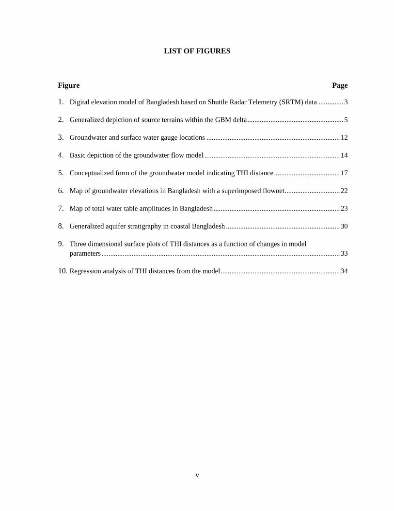
1. Digital elevation model of Bangladesh based on Shuttle Radar Telemetry (SRTM) data .............. 3
2. Generalized depiction of source terrains within the GBM delta ...................................................... 5
3. Groundwater and surface water gauge locations ........................................................................... 12
4. Basic depiction of the groundwater flow model ............................................................................ 14
5. Conceptualized form of the groundwater model indicating THI distance ..................................... 17
6. Map of groundwater elevations in Bangladesh with a superimposed flownet ............................... 22
7. Map of total water table amplitudes in Bangladesh ....................................................................... 23
8. Generalized aquifer stratigraphy in coastal Bangladesh ................................................................ 30
9. Three dimensional surface plots of THI distances as a function of changes in model
parameters ...................................................................................................................................... 33
10. Regression analysis of THI distances from the model ................................................................... 34
1
CHAPTER I
INTRODUCTION
The global community has experienced growing pressures – both physical and social –
from climate change and its associated effects. Low-lying deltaic regions have been particularly
impacted by climate change (Nicholls et al., 2007). These regions are often characterized by the
tight coupling of the natural and human systems with even small perturbations to one system
affecting the other. Consequently, low-lying deltaic regions are active sites of human migration in
the face of climate change and more specifically sea level rise. Recent studies found that previous
estimates of sea level rise (18-59 cm by 2100) made by the IPCC Fourth Assessment Report
(Meehl et al., 2007) are conservative. A summary (National Research Council, 2010) of these
studies finds sea level rise estimates ranging from 56 to 200 cm by 2100. Coastal regions are
becoming increasingly more susceptible to inundation and waterlogging, erosion, and ecosystem
disturbances through both sustained and catastrophic weather events. Coastal groundwater systems
are particularly susceptible to sea level rise through coastal inundation, especially in regions with
expansive and actively prograding deltas such as the Ganges-Brahmaputra-Meghna (GBM) delta
(commonly referred to as the Bengal Basin). These deltas are often characterized by regional
aquifer systems and are largely low-lying and topographically homogenous. Small changes in sea
level may result in significant perturbations to the deltaic system and an increase in the potential
for aquifer salinization (Nicholls and Cazenave, 2010). In addition, population growth, related
groundwater abstraction, and expansion of aquaculture may exacerbate the problem (Primavera,
1997; Vengosh, 2003).

2
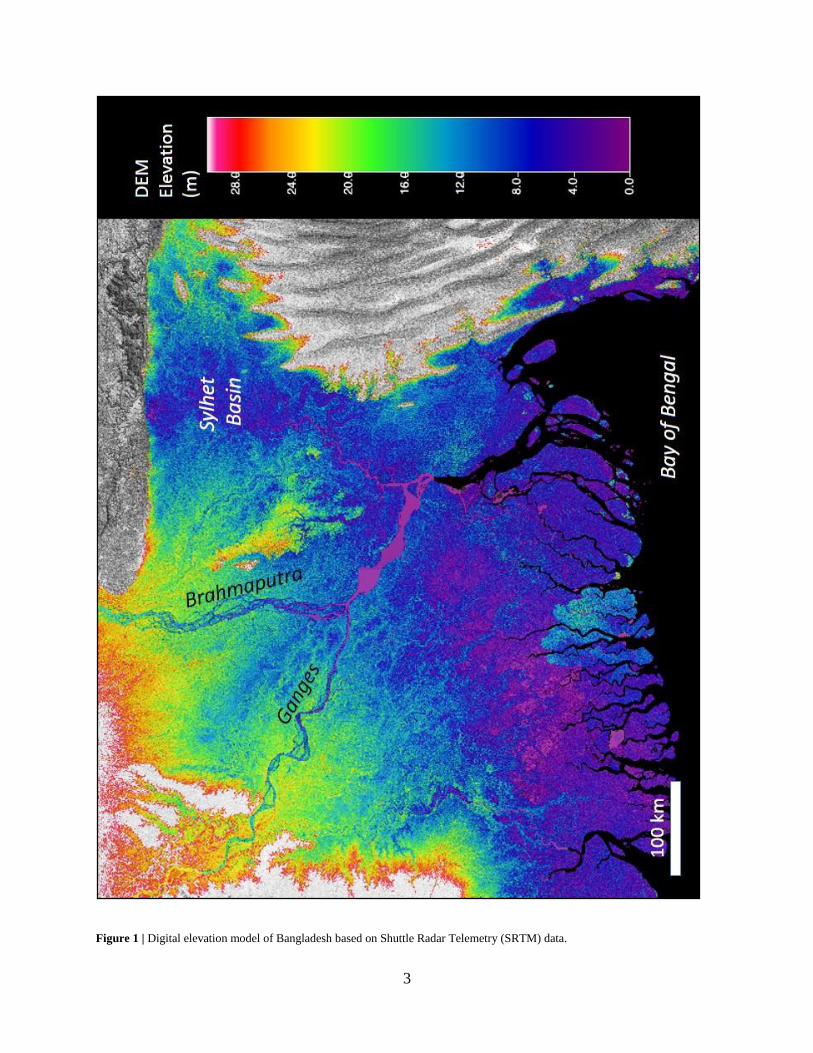
The Bengal Basin is particularly susceptible to sea level rise and related aquifer salinization
as much of it lies within 3 m of sea level (Fig. 1). In particular, the southwest region has been
identified as one of the areas in greatest need of augmentation to freshwater stores (WARPO,
2001). The aquifers appear to be regionally saline (BGS and DPHE, 2001; WARPO, 2001; Bahar
and Reza, 2010); however, local instances of freshwater lenses do occur. As a result, the region
relies primarily on trapped wet season precipitation (WARPO, 2001). These resources are highly
vulnerable to waterborne pathogens (Karim, 2010) and destruction by storm surge (Dasgupta et
al., 2010). Filtration of pathogens has been somewhat successful (Karim, 2010); though, storm
surge continues to be a concern (e.g. Cyclone Aila, 2009; Cyclone Sidr, 2007). Under these
stressed conditions, even local freshwater lenses provide relief.
Understanding the origin and mechanism of aquifer recharge is paramount in determining
the effect of climate change and sea level rise on the groundwater. A study of groundwater salinity
in Comilla in eastern Bangladesh suggests a connate origin to brackish groundwater (Hoque et al.,
2003). Little work has been done, however, to understand the origin of brackish groundwater in
southwest Bengal despite the fact that groundwater amplitudes suggest a tidal modulation of
groundwater in coastal Bangladesh. Furthermore, it is unclear how human alterations such as
poldering (embanking of land to prevent inundation at high tide) and saline aquaculture may affect
the underlying aquifer systems. Regardless of the cause, diminished access to freshwater will
continue to stress the region in the near future and potentially lead to temporary or permanent
migration. The goal of this research effort is to explore and develop a better understanding of
groundwater and surface water interactions in southwest Bengal through computer modeling.
3
Figure 1 | Digital elevation model of Bangladesh based on Shuttle Radar Telemetry (SRTM) data.
4
The Bengal Basin
Geography
The Bengal Basin lies at an active plate margin between the Indian, Burman, and Tibetan
(Eurasian) plates. The basin is nested within the larger GBM basin and consists predominantly of
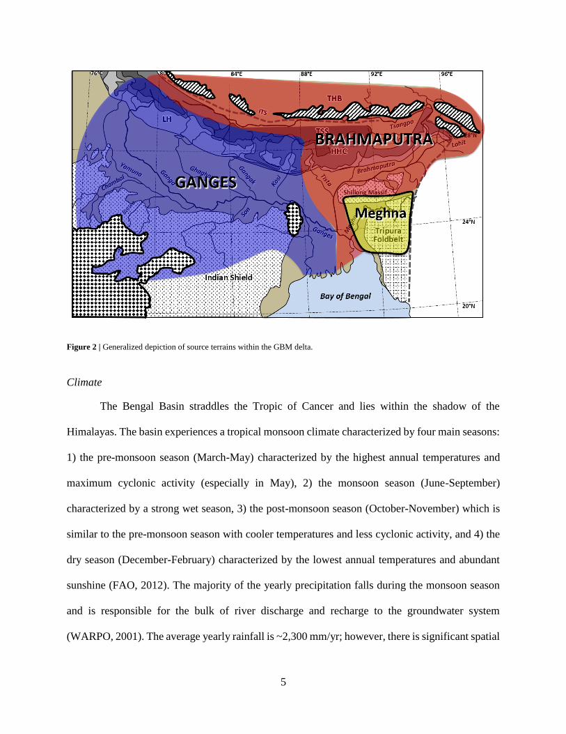
alluvial sediments deposited by the Ganges and Brahmaputra (Fig. 2). The region is bounded by
the Himalayas to the distant north and northwest, the Shillong Massif to the immediate north and
northeast, the Indo-Burman ranges to the east, the Indian Craton to the west, and the Bay of Bengal
to the south (Morgan and McIntire, 1959).
Three major river systems dissect the Bengal Basin – the Ganges, Brahmaputra, and
Meghna. The Ganges originates in the Himalayas in the state of Uttarkhand in India and flows
southwest, joining tributary streams from Bhutan and other parts of India before crossing into
Bangladesh ~18 km downstream of Farakka. The Brahmaputra originates on the north side of the
Himalayas in China and flows east along the Tibetan Plateau before turning south and then
southwest joining streams from Bhutan and eastern India and eventually crossing into Bangladesh
~50 km west of Rangpur. The Meghna originates in the state of Assam in eastern India and flows
southwest toward the Sylhet Basin in Bangladesh. The Ganges and Brahmaputra meet ~25 km
northwest of Faridpur and then continue another 100 km downstream where they combine with
the Upper Meghna northwest of Chandpur. The Lower Meghna, one of the biggest rivers in the
world, then continues ~150 km to the Bay of Bengal (Fig. 2). The combined GBM system drains
an area of 1.75 million km2 and has a combined river length of 24,000 km2 (FAO, 2012).
5
Figure 2 | Generalized depiction of source terrains within the GBM delta.
Climate
The Bengal Basin straddles the Tropic of Cancer and lies within the shadow of the
Himalayas. The basin experiences a tropical monsoon climate characterized by four main seasons:
1) the pre-monsoon season (March-May) characterized by the highest annual temperatures and
maximum cyclonic activity (especially in May), 2) the monsoon season (June-September)
characterized by a strong wet season, 3) the post-monsoon season (October-November) which is
similar to the pre-monsoon season with cooler temperatures and less cyclonic activity, and 4) the
dry season (December-February) characterized by the lowest annual temperatures and abundant
sunshine (FAO, 2012). The majority of the yearly precipitation falls during the monsoon season
and is responsible for the bulk of river discharge and recharge to the groundwater system
(WARPO, 2001). The average yearly rainfall is ~2,300 mm/yr; however, there is significant spatial
6
variability within the basin. The highest mean precipitation rates (~5,500 mm/yr) occur in the
northeast, while the lowest mean precipitation rates (~1,000 mm/yr) occur in the northwest.
Temperatures range from 4°C in the dry season to 43°C in the pre-monsoon season with a mean
temperature of 25°C. Humidity ranges from 60% during the dry season to 98% during the monsoon
season (FAO, 2012).
Geology & Hydrology
The evolution of the Bengal Basin throughout the Late Quaternary has been controlled by
variations in tectonics and subsidence, climate, and sea level (Umitsu, 1993; Goodbred and Kuehl,
2000a; Goodbred and Kuehl, 2000b). The compounding effect of these variations has resulted in
a highly dynamic, complex deltaic environment with significant stratigraphic and aquifer
variability. While the tectonics of the region are poorly understood, the uplift of the Himalayas
and the Indo-Burman Ranges most certainly amplified the southwest monsoon and the associated
wet season with water and sediment discharges increasing concurrently (Alam et al., 2003).
Modern delta formation began ~11 ka when the basin became flooded as a result of rising sea
levels and a strengthened southwest monsoon (Goodbred and Kuehl, 2000a). Holocene deposition
alone has produced a deltaic feature with a subaerial surface area of 110,000 km2 (Kuehl et al.,
2005). Furthermore, sea level fluctuations have controlled the prevalence of deposition and erosion
throughout the basin with marine transgressions shifting the sediment depocenters inland and
marine regressions resulting in the converse. Present day hydrostratigraphy is closely tied to these
paleo-sea level fluctuations.
The most recent major regression cycle ended ~20 ka at the Last Glacial Maximum (LGM).
Contemporaneously, main river channels became incised to near base level (~120 m below sea
7
level) and interfluves were weathered and oxidized to depths of tens of meters. Thus, the LGM
lowstand resulted in a basin-wide, thick and relatively impermeable paleosol dissected by deeply
incised Pleistocene channels (McArthur et al., 2008). Following the LGM, sea level predominantly
transgressed; however, episodic regressions most likely occurred causing interbedded silt and clay
aquitards within productive, sandy aquifers (Umitsu, 1993). These aquitards become more
prominent nearer to the coast (Ravenscroft and McArthur, 2004). Below both the Pleistocene
paleosol terraces and the Holocene floodplains, alluvial sedimentation has resulted in highly
productive aquifer systems. The shallowest aquifers are typically found within 10-60 m depth
while the deepest are at >300 m depth. Brackish aquifers exist in coastal regions of Bangladesh
(Ahmed et al., 2004; Ravenscroft and McArthur, 2004; Ravenscroft et al., 2005) and in isolated
pockets further inland (Hoque et al., 2003).
Presently, the GBM combined average water discharge is among the highest in the world
with peak discharges of 100,000 m3/s from the Brahmaputra, 75,000 m3/s from the Ganges, and
20,000 m3/s from the Upper Meghna, and 160,000 m3/s from the Lower Meghna (FAO, 2012).
The Ganges and Brahmaputra systems drain the Himalayas and the Tibetan Plateau and provide
the bulk of the sediment to the basin with a sediment flux of 316 million tons/yr and 721 million
tons/yr respectively (Islam et al., 1999). The total sediment load is ~1037 million tons/yr, of which
~525 million tons/yr is deposited in the lower delta while the remainder (~512 million tons/yr)
offsets subsidence through floodplain deposition and riverbed aggradation (Islam et al., 1999). The
modern delta continues to prograde into the Bay of Bengal, resulting in a combined subaerial and
submarine surface area of 140,000 km2 (Kuehl et al., 2005). Active deltaic feature formation
occurs in the eastern delta, while the western delta receives little fluvial input and is predominantly
tidal (Umitsu, 1993). Much of the sediment is reworked and redistributed within the delta as a
8
result of strong semidiurnal tides with a range of 1.9 m in the west and 2.8 m in the east (Barua,
1990). As the tides propagate inland, the range can increase to as much as 5 m (Kuehl et al., 2005).
Climate Change & Human Conflict
The GBM river basin spans 5 international boarders – Bangladesh, Bhutan, China, India,
and Nepal. The basin is home to an estimated 630 million people making it one of the most densely
populated and poorest regions of the world (FAO, 2012). The Bengal Basin is often cited as being
highly vulnerable to the effects of climate change and sea level rise through tropical cyclones and
storm surges (Ali, 1996; Ali, 1999; IPCC, 2007; Dasgupta et al., 2010). The basin is relatively
inactive in comparison with other tropical cyclone basins; however, its position at the confluence
of the GBM system, high population density, lack of resources, and limited ability for preparation
and management results in greater impacts during even small cyclonic events. The IPCC Fourth
Assessment Report suggests that the frequency of these extreme weather events will increase
(Meehl et al., 2007). This may result in cyclonic events becoming more frequent within the basin.
However, a special report discusses the uncertainty in changes to extreme weather patterns at the
local level (IPCC, 2012). Regardless, the impact of cyclonic storms will continue to increase in
the Bengal Basin through population growth, continued progradation of the delta, and decreased
resilience to storm surge through anthropogenic perturbations to the system.
Not only do humans affect the local environment, but they are also influenced by a number
of environmental stressors – many of which are directly related to sea level rise and the impacts
on coastal regions. Most recently, Cyclone Sidr (2007) and Cyclone Aila (2009) both caused
catastrophic losses to human life, livestock, and land through embankment failure (United Nations,
2007; United Nations, 2010). Cyclone Aila caused large portions of the coastal populations to be

9
displaced both locally (temporary relocation onto embankments) and regionally (migration into
cities) (Mehedi, 2010; Kartiki, 2011). Furthermore, anthropogenic perturbations such as poldering
and conversion of land to aquaculture may destabilize coastal systems, resulting in decreased
resilience to storm surge (e.g., increased flooding – both sustained and temporary, land subsidence,
and salinization of freshwater resources).
Research in the Bengal Basin
Research in the Bengal Basin increased significantly in the 1990s following the
identification of the widespread occurrence of arsenic in the groundwater. Since then, much
research has been done concerning the origin and transport of arsenic in groundwater (Acharyya
et al., 2000; BGS and DPHE, 2001; Kinniburgh and Kosmus, 2002; Harvey et al., 2002; Gaus et
al., 2003; Ahmed et al., 2004; Ravenscroft et al., 2005; Harvey et al., 2006; Michael and Voss,
2008; McArthur et al., 2008; McArthur et al., 2011). The majority of this research focuses on
regional flow patterns in an attempt to discern the cause of the mobilization of arsenic and the
spatial arrangement of the contaminated aquifers. Very few studies (Harvey et al., 2002; Harvey
et al., 2006) have focused on local groundwater flow paths. Regional analyses often characterize
the aquifer system into regionally extensive, distinct layers and offer generalized depictions of
groundwater flow. Such analyses prove useful for water resource planning at the government and
aid organization level; however, the stratigraphy of the basin is highly variable due in part to a
highly active river system with a high sediment load situated in a tectonically active region
(Goodbred et al., 2003; Kuehl et al., 2005). While localized studies provide point data and help
develop a more complete understanding at the regional level, economic resources are limited. The
result is that groundwater flow and water chemistry data is severely limited in the Bengal Basin.

10
Other research has been done on soil salinization through aquaculture and agriculture
(Mondal et al., 2001; Thornton et al., 2003; Azad et al., 2009; Chowdhury et al., 2011). These
studies focus on salinization of the soil through conversion of rice paddies into saline shrimp farms.
Rice paddy fields are inundated with saline water from either presently saline groundwater that is
pumped onto the surface or water from tidal channels through the use of sluice gates or basic
diesel-run portable pumps. Such practices may induce a downward gradient resulting in saline
surface waters contaminating freshwater resources – both local freshwater lenses and regionally
fresh aquifer systems. The most comprehensive aquifer study (BGS and DPHE, 2001) analyzed
3534 tube wells in Bangladesh or approximately 0.03-0.05% of all active tube wells within the
country. Care was taken in order to ensure a representative sample was selected, but often flooding
and lack of vehicular access prevented development of an ideal sampling schema.
Many of the aforementioned studies acknowledge the presence of brackish groundwater in
the coastal region and suggest a connate origin despite the lack of surface water and groundwater
data in southwest Bengal. In this study, we model the surface water and groundwater system over
a realistic range of parameters. The results suggest that the brackish groundwater may not be
entirely of connate origin and in fact could be connected to the overlying tidal network.
11
CHAPTER II
METHODS
Water Level Data
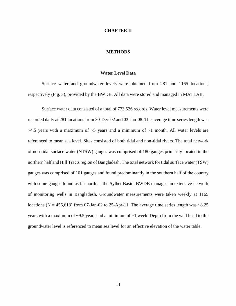
Surface water and groundwater levels were obtained from 281 and 1165 locations,
respectively (Fig. 3), provided by the BWDB. All data were stored and managed in MATLAB.
Surface water data consisted of a total of 773,526 records. Water level measurements were
recorded daily at 281 locations from 30-Dec-02 and 03-Jan-08. The average time series length was
~4.5 years with a maximum of ~5 years and a minimum of ~1 month. All water levels are
referenced to mean sea level. Sites consisted of both tidal and non-tidal rivers. The total network
of non-tidal surface water (NTSW) gauges was comprised of 180 gauges primarily located in the
northern half and Hill Tracts region of Bangladesh. The total network for tidal surface water (TSW)
gauges was comprised of 101 gauges and found predominantly in the southern half of the country
with some gauges found as far north as the Sylhet Basin. BWDB manages an extensive network
of monitoring wells in Bangladesh. Groundwater measurements were taken weekly at 1165
locations (N = 456,613) from 07-Jan-02 to 25-Apr-11. The average time series length was ~8.25
years with a maximum of ~9.5 years and a minimum of ~1 week. Depth from the well head to the
groundwater level is referenced to mean sea level for an effective elevation of the water table.
12
Figure 3 | Groundwater and surface water gauge locations. A. Plot of all groundwater well gauges that were used for hydrologic
analysis. B. Plot of all non-tidal surface water gauges that were used for analysis. C. Plot of all tidal surface water gauges that were
used for analysis.

13
Geospatial Data
Data for analysis in ArcGIS was compiled from multiple sources. All data were referenced
to the WGS 1984 horizontal datum. Political boundary data were obtained from GADM database
of Global Administrative Areas (GADM, 2012). Streamlines at a resolution of 15 arc-seconds and
a digital elevation model (DEM) of 3 arc-seconds were obtained from HydroSHEDS (Lehner et
al., 2008). All geologic data were obtained from the USGS (Persits et al., 2001). The built-in
ArcGIS aerial imagery was used as a base map (Esri et al., 2012). (Table 1)
Table 1 | Geospatial data and sources. Data used for contextual analysis of surface water and groundwater interactions.
Data Data Type Description Source
Aerial
Imagery Imagery Aerial imagery for entire study area. Esri
Digital
Elevation
Model
DEM Digital elevation model for Bangladesh from SRTM data. HydroSHEDS
(Lehner et al., 2008)
Geology of
Bangladesh Geology
Generalized elevations, faults and tectonic contacts, surface geology,
Bouguer gravity anomaly, aeromagnetic anomaly, physiographic
features, tectonic features
USGS
Political
Boundaries Boundary
Boundaries for countries, divisions, regions, districts, and sub-
districts GADM
Streams Hydrology Streamlines for Southeast Asia HydroSHEDS
(Lehner et al., 2008)
Geospatial Analysis
Water level data from the BWDB were processed in MATLAB and then imported into
ArcGIS for analysis. In MATLAB, groundwater and non-tidal surface water elevations were
aggregated in order to depict the groundwater table. Monthly mean head, total mean head, and
total amplitude (difference between the maximum head and minimum head over the entire period
of record) at each location was calculated. These vectors were then imported into ArcGIS and
georeferenced using the latitude and longitude of the associated gauge. The data were then
14
rasterized through ordinary kriging and fit to a spherical semivariogram using the Geostatistical
Analyst extension in ArcGIS. Rasterized water table elevations were then used to construct a flow
net using ArcHydro Groundwater.
Construction of the Groundwater Model
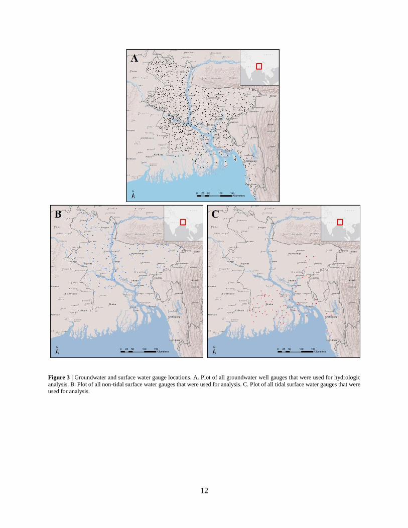
A one-dimensional groundwater flow model between two tidal river channels in MATLAB
(Fig. 4) was employed to analyze groundwater behaviors in southwest Bengal. The model depicted
head variations in the horizontal direction as a result of tidal river fluctuations. The tidal rivers
served as the boundary conditions fluctuating between a maximum (TR) and minimum (-TR) tidal
extent while groundwater flow equations governed at 0 < x < X. The space between the tidal
channels was subdivided into n nodes.
Figure 4 | Basic depiction of the groundwater flow model. Tidal channels are located at x < 0 and x > X and fluctuate between TR
and -TR. Groundwater flow equations govern from 0 < x < X.
0 X-TR
0
TR
Island Width
Ele
vation (
above b
asele
vel)
Groundwater Head
Embankment Surface
Ground Surface
Channel Boundary

15
The tidal channels (boundary conditions) were defined using sinusoids with a period of 12
hours for the solar tidal cycle, 12.42 hours for the lunar tidal cycles, and 8760 hours (1 year) for
the seasonal monsoon (Equation 1).
ℎ𝑏𝑐 = sin 𝑎𝑙 (2𝜋
𝑡
12.42) + sin 𝑎𝑠 (2𝜋
𝑡
12) + sin 𝑎𝑚 (2𝜋
𝑡
8760+
3𝜋
4) (1)
Where hbc is the head at the boundary condition, al, as, and am are the lunar, solar, and wet season
components of the tidal amplitude, respectively, and t is time.
Flow within the aquifer was governed by Darcy’s Law (Equation 2).
𝜕ℎ
𝜕𝑡=
1
𝑆
𝜕
𝜕𝑥(𝑇
𝜕ℎ
𝜕𝑥) +
𝑅𝑒
𝑆 (2)
Where h is groundwater head, t is time, T is transmissivity, S is storativity, x is horizontal space,
and Re is effective surface recharge.
Transmissivity was varied to reflect differences in aquifer and channel characteristics over
horizontal space. The partial derivative of 𝜕
𝜕𝑥(𝑇
𝜕ℎ
𝜕𝑥) was approximated as
(𝑇𝜕ℎ𝜕𝑥
)𝑖+1
2⁄− (𝑇
𝜕ℎ𝜕𝑥
)𝑖−1
2⁄
∆𝑥
The derivatives of the internodes were then approximated as
(𝑇𝜕ℎ
𝜕𝑥)
𝑖+12⁄
= √𝑇𝑖𝑇𝑖+1 ℎ𝑖+1 − ℎ𝑖
∆𝑥
(𝑇𝜕ℎ
𝜕𝑥)
𝑖−12⁄
= √𝑇𝑖𝑇𝑖−1 ℎ𝑖−1 − ℎ𝑖
∆𝑥

16
With transmissivity approximated using the geometric mean of the bounding nodes √𝑇𝑖𝑇𝑖−1.
Equation 2 was then approximated using a backward difference (implicit) approximation
(Equation 3).
ℎ𝑖
𝑗+1− ℎ𝑖
𝑗
∆𝑡=
𝑇𝑖+12⁄ ℎ𝑖+1
𝑗+1− (𝑇𝑖+1
2⁄ + 𝑇𝑖−12⁄ ) ℎ𝑖
𝑗+1+ 𝑇𝑖+1
2⁄ ℎ𝑖−1𝑗+1
𝑆(∆𝑥)2+
𝑅𝑒
𝑆 (3)
Where j is the time dimension and i is the spatial dimension.
The equation was then written in matrix form and solved by placing all unknowns (heads at time
j+1) on the left and all knowns (heads at time j) on the right (Equation 4):
𝐴ℎ𝑗+1 = ℎ𝑗 +
𝑅𝑒
𝑆 (4)
Where A is the sparse matrix with main diagonal element of 1+2r and sub- and super-diagonal
elements of –r. Here, r is a vector of coefficients associated with each groundwater head term.
𝑟 =𝑇∆𝑡
𝑆∆𝑥2
The model was then run for a specified amount of time t and values of head for all times and nodes
were recorded.
Effective surface recharge varied temporally with R0 occurring during the dry season
(R=0), R1 occurring during the monsoonal months June and July, and R2 occurring during the
monsoonal months August and September. Nearly all of precipitation falls from June to
September; however, the bulk of wet season recharge comes in June and July (R1 > R2). Monsoonal
precipitation data from 1980 to 2010 for Khulna, Bangladesh (Bangladesh Meteorological
17
Department, 2012) were aggregated and the mean was used to provide appropriate monthly
precipitation values as a percentage of yearly precipitation. Monthly precipitation values were then
converted to effective monthly recharge rates by using interpolated data from prior studies
(Shamsudduha et al., 2011). The study provided a yearly effective recharge rate for the region
which was then divided into monthly precipitation (June through September) using the percentage
of total yearly precipitation.
MATLAB Analysis
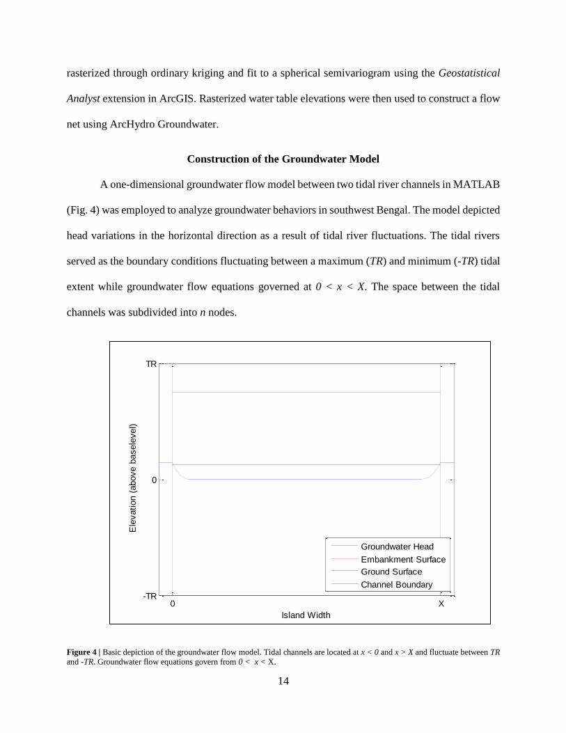
The main aim of this study was to determine the length scale x̄ of tidal influence on the
groundwater head, referred to herein as tidal head incursion (THI) distance (Fig. 5).
Figure 5 | Conceptualized form of the groundwater model indicating THI distance. The point at which tidal influences become
negligible is delineated by xbar.
0 xbar X-TR
0
TR
Island Width
Ele
vation (
above b
asele
vel)
Groundwater Head
Embankment Surface
Ground Surface
Channel Boundary
18
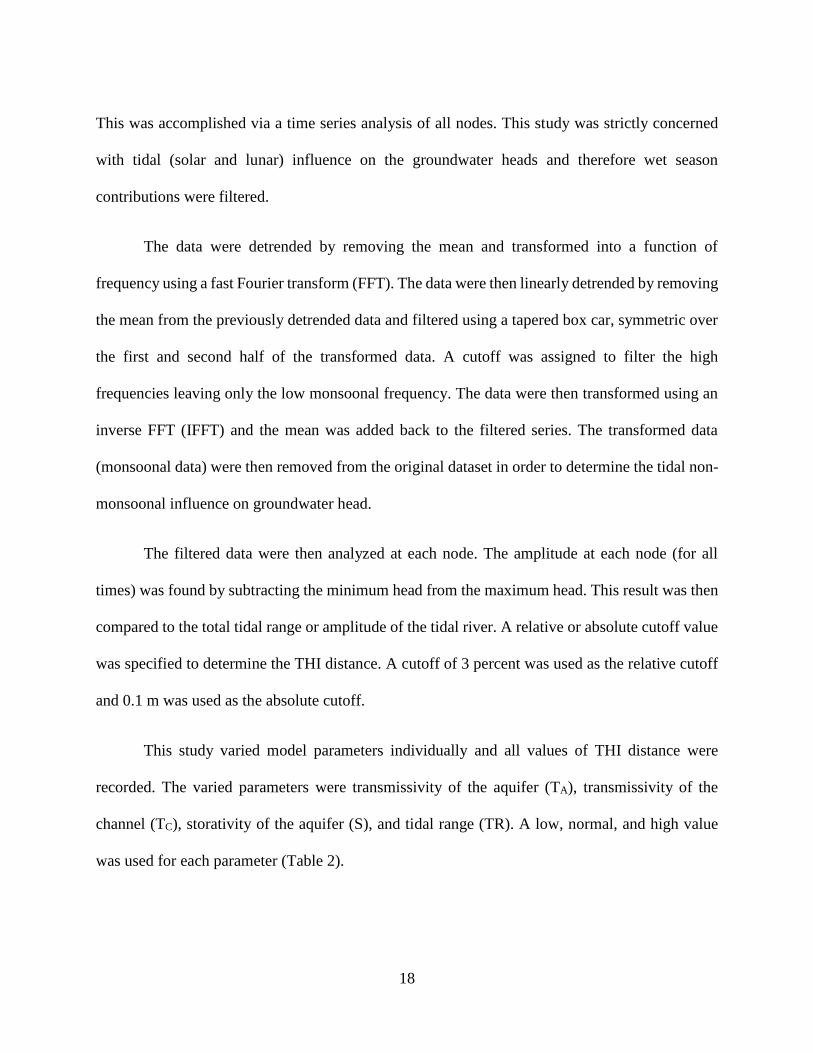
This was accomplished via a time series analysis of all nodes. This study was strictly concerned
with tidal (solar and lunar) influence on the groundwater heads and therefore wet season
contributions were filtered.
The data were detrended by removing the mean and transformed into a function of
frequency using a fast Fourier transform (FFT). The data were then linearly detrended by removing
the mean from the previously detrended data and filtered using a tapered box car, symmetric over
the first and second half of the transformed data. A cutoff was assigned to filter the high
frequencies leaving only the low monsoonal frequency. The data were then transformed using an
inverse FFT (IFFT) and the mean was added back to the filtered series. The transformed data
(monsoonal data) were then removed from the original dataset in order to determine the tidal non-
monsoonal influence on groundwater head.
The filtered data were then analyzed at each node. The amplitude at each node (for all
times) was found by subtracting the minimum head from the maximum head. This result was then
compared to the total tidal range or amplitude of the tidal river. A relative or absolute cutoff value
was specified to determine the THI distance. A cutoff of 3 percent was used as the relative cutoff
and 0.1 m was used as the absolute cutoff.
This study varied model parameters individually and all values of THI distance were
recorded. The varied parameters were transmissivity of the aquifer (TA), transmissivity of the
channel (TC), storativity of the aquifer (S), and tidal range (TR). A low, normal, and high value
was used for each parameter (Table 2).

19
Table 2 | Range of values used for groundwater model parameters.
Notation Parameter Unit Low (1) Norm (2) High (3)
𝑻𝑨 Aquifer Transmissivity 𝑚2
ℎ⁄ 0.5 10 50
𝑻𝑪 Channel Transmissivity 𝑚2
ℎ⁄ 0.3 10 75
𝑺 Storativity 𝑉𝑉⁄ 0.001 0.01 0.1
𝑻𝑹 Tidal Range 𝑚 2 3 4
Channel transmissivity (TC) was defined within 50 m of the tidal channel while aquifer
transmissivity (TA) was defined for all remaining nodes. Aquifer transmissivity values ranged from
a very fine grained to a medium grained sand in a moderately thick aquifer (~20 m). Channel
transmissivity was similar, with the exception of both the low and high values being more extreme
to encompass the possibility for channel aggradation and scouring respectively. Storativity was
defined by classic values for a confined, semi-confined, and unconfined system. Tidal range values
varied from 2 to 4 m, which is representative of the tidal system in Bangladesh.
All parameter combinations were tested and the associated values of THI distance were
recorded in a table. The table was then color-contoured to facilitate identification of patterns.
20
CHAPTER III
RESULTS
Geospatial Results
Water table elevations (in meters above mean sea level; Fig. 6) exhibited a general decline
from northwest to southeast. Elevations were highest in the northwestern region of Bangladesh,
ranging from 15 to 70 m. Elevations fell at a rate of 0.3 m/km in the direction of the Shillong
Massif. The elevations in the central portion of the country, excluding Dhaka, ranged from 3 to 15
m. The water table declined at a more modest rate of 0.03 m/km from the southern extent of the
Shillong Massif toward the confluence of the Jamuna and Ganges Rivers. The Sylhet Basin
northeast of Dhaka city was characterized by lower water table elevations as compared to the
adjacent areas east and west. The region around Dhaka city was characterized by a significant cone
of depression with water table elevations of -15 to -35 m. Flow was radially inward towards the
city center as indicated by a drop in groundwater head at a rate of ~1.5 m/km. The region west of
Dhaka also had smaller cones of depression with radially inward flow indicated by a drop in
groundwater head at a rate of <1 m/km. Coastal water table elevations in the south and southwest
were spatially coherent with typical values at <1 m and a maximum of ~1.75 m near Khulna city.
The water table sloped more gently at 0.015 m/km south of Khulna. The region north and east of
the GBM river mouth had higher water table elevations of 3 to 4 m and declined quickly at 0.1
m/km toward the southwest. The coastal area west of the GBM river mouth was defined by slightly
higher water table elevations at the coast compared to the inland tidally drained system, resulting
in flow from south to north or an inland direction. The water table in the Hill Tracts region near
21
Chittagong city was defined by more significant topography resulting in elevations of >10 m and
declines at the rate of 0.3 m/km toward the west. Anomalously high values were found in the
extreme southwest region due to low gauge density in the Sundarbans.
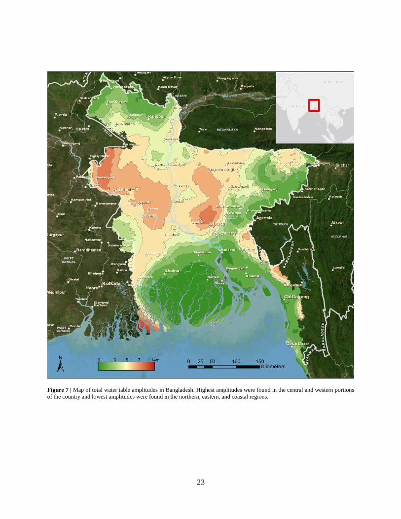
A majority of water table amplitudes (difference between the maximum head and minimum
head over the entire period of record for each well; Fig. 7) varied from 0.02 to 14 m with
anomalously high values (>20 m) in northwest Bangladesh and around Dhaka city. The highest
amplitudes were found in the northwest portion of the country. Significant amplitudes were found
north of Dhaka city and in western portions of the Rajshahi and Khulna divisions. The lowest
amplitudes were less contiguous and found in the northern portion of the country west of the
Shillong Massif, southeast Sylhet division, and extensively in the tidal dominated coastal region
from Khulna city to Chittagong city. Once again, anomalously high values were found in the
extreme southwest region due to low gauge density in the Sundarbans.

22
Figure 6 | Map of groundwater elevations in Bangladesh with a superimposed flownet. Water table elevations are highest in the
northwest region of the country (15 to 70 m) and lowest at the coast (0-2 m). A significant cone of depression (-15 to -35 m) is
evident in Dhaka. Groundwater flow at the coast west of the GBM mouth is in an inland direction.
23
Figure 7 | Map of total water table amplitudes in Bangladesh. Highest amplitudes were found in the central and western portions
of the country and lowest amplitudes were found in the northern, eastern, and coastal regions.

24
Groundwater Model Results
The groundwater model described the groundwater behaviors of the tidally dominated
region south of Khulna. THI distance outputs from the model are shown in Table 3. The table
displays THI distance for a relative cutoff (3%) below the diagonal line and THI distance for
absolute cutoff (0.1 m) above the diagonal line. The table is color-contoured from green (low
values of THI distance) to red (high values of THI distance).
Table 3 | THI distance as a function of aquifer transmissivity, channel transmissivity, storativity, and tidal range. A low (1), normal
(2), and high (3) value for each parameter was used (see Table 2 for exact values). Parameters are co-varied and THI distances are
shown in the grid. A cutoff of 3 percent was used as the relative cutoff and 0.1 m was used as the absolute cutoff.
TA1 TA2 TA3 TC1 TC2 TC3 S1 S2 S3 TR1 TR2 TR3
TA1 40 80 80 200 80 40 80 80 80
Ab
solu
te Cu
toff
TA2 140 260 280 1000 260 80 220 260 280
TA3 320 580 600 1000 580 140 520 580 640
TC1 40 140 340 780 140 0 100 140 160
TC2 80 260 600 1000 260 80 220 260 280
TC3 80 280 620 1000 280 100 240 280 300
S1 200 1000 1000 820 1000 1000 760 1000 1000
S2 80 260 600 140 260 280 220 260 280
S3 40 80 160 0 80 100 60 80 80
TR1 80 260 600 140 260 280 1000 260 80
TR2 80 260 600 140 260 280 1000 260 80
TR3 80 260 600 140 260 280 1000 260 80
Relative Cutoff
THI distances for relative cutoff were highest at low values of storativity (S1, S=0.001, i.e.
confined) and moderately high for high aquifer transmissivity values (TA3, TA = 240 m2/d, i.e. well
sorted sand). THI distances were lowest at low channel transmissivities (TC1, TC = 2.4 m2/d, i.e.
25
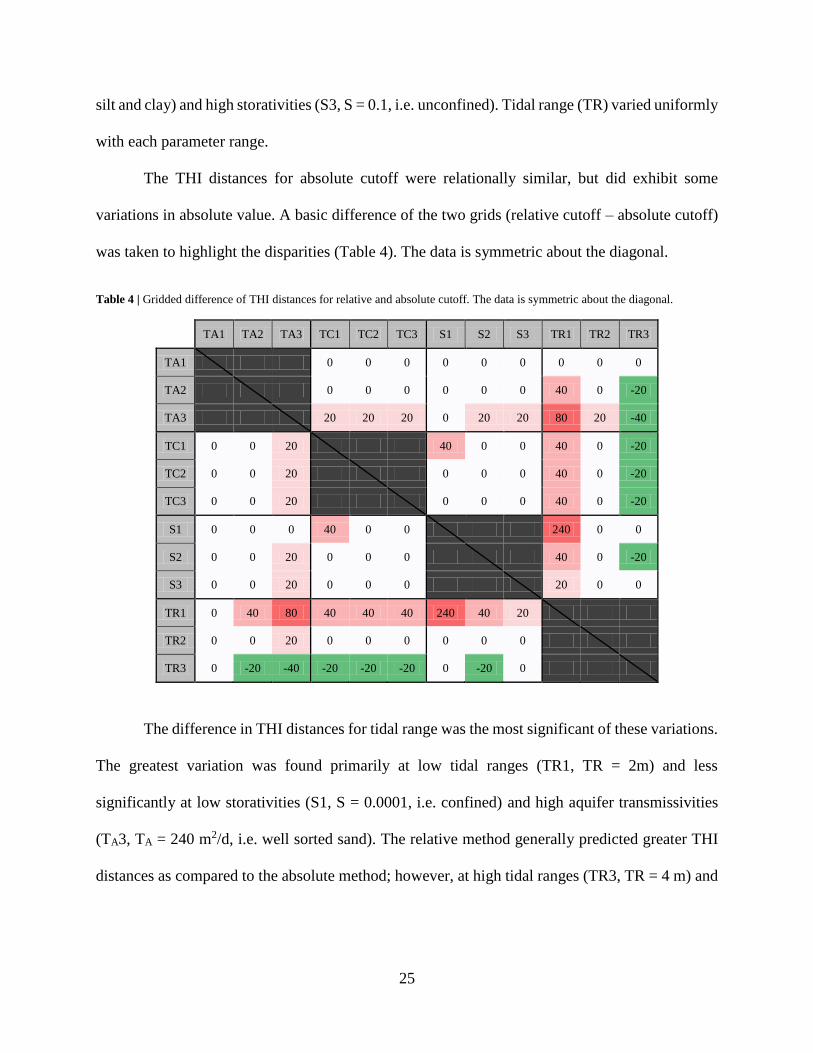
silt and clay) and high storativities (S3, S = 0.1, i.e. unconfined). Tidal range (TR) varied uniformly
with each parameter range.
The THI distances for absolute cutoff were relationally similar, but did exhibit some
variations in absolute value. A basic difference of the two grids (relative cutoff – absolute cutoff)
was taken to highlight the disparities (Table 4). The data is symmetric about the diagonal.
Table 4 | Gridded difference of THI distances for relative and absolute cutoff. The data is symmetric about the diagonal.
TA1 TA2 TA3 TC1 TC2 TC3 S1 S2 S3 TR1 TR2 TR3
TA1 0 0 0 0 0 0 0 0 0
TA2 0 0 0 0 0 0 40 0 -20
TA3 20 20 20 0 20 20 80 20 -40
TC1 0 0 20 40 0 0 40 0 -20
TC2 0 0 20 0 0 0 40 0 -20
TC3 0 0 20 0 0 0 40 0 -20
S1 0 0 0 40 0 0 240 0 0
S2 0 0 20 0 0 0 40 0 -20
S3 0 0 20 0 0 0 20 0 0
TR1 0 40 80 40 40 40 240 40 20
TR2 0 0 20 0 0 0 0 0 0
TR3 0 -20 -40 -20 -20 -20 0 -20 0
The difference in THI distances for tidal range was the most significant of these variations.
The greatest variation was found primarily at low tidal ranges (TR1, TR = 2m) and less
significantly at low storativities (S1, S = 0.0001, i.e. confined) and high aquifer transmissivities
(TA3, TA = 240 m2/d, i.e. well sorted sand). The relative method generally predicted greater THI
distances as compared to the absolute method; however, at high tidal ranges (TR3, TR = 4 m) and

26
low aquifer transmissivities (TA1, TA = 12 m2/d, i.e. silt and clay) the absolute method predicted
greater THI distances.
27
CHAPTER IV
DISCUSSION
Groundwater and Surface Water Interactions in the Bengal Basin
Mean water table elevations throughout the country decline from northwest to southeast in
relation to topography and local water table elevations. Significant water table depressions exist
throughout the central portion of the country as a result of dry season irrigation (Shamsudduha et
al., 2009; Shamsudduha et al., 2011; Shamsudduha et al., 2012). Generalized flow paths are from
northwest to southeast with flow radially inward toward the centers of the multiple inland basins
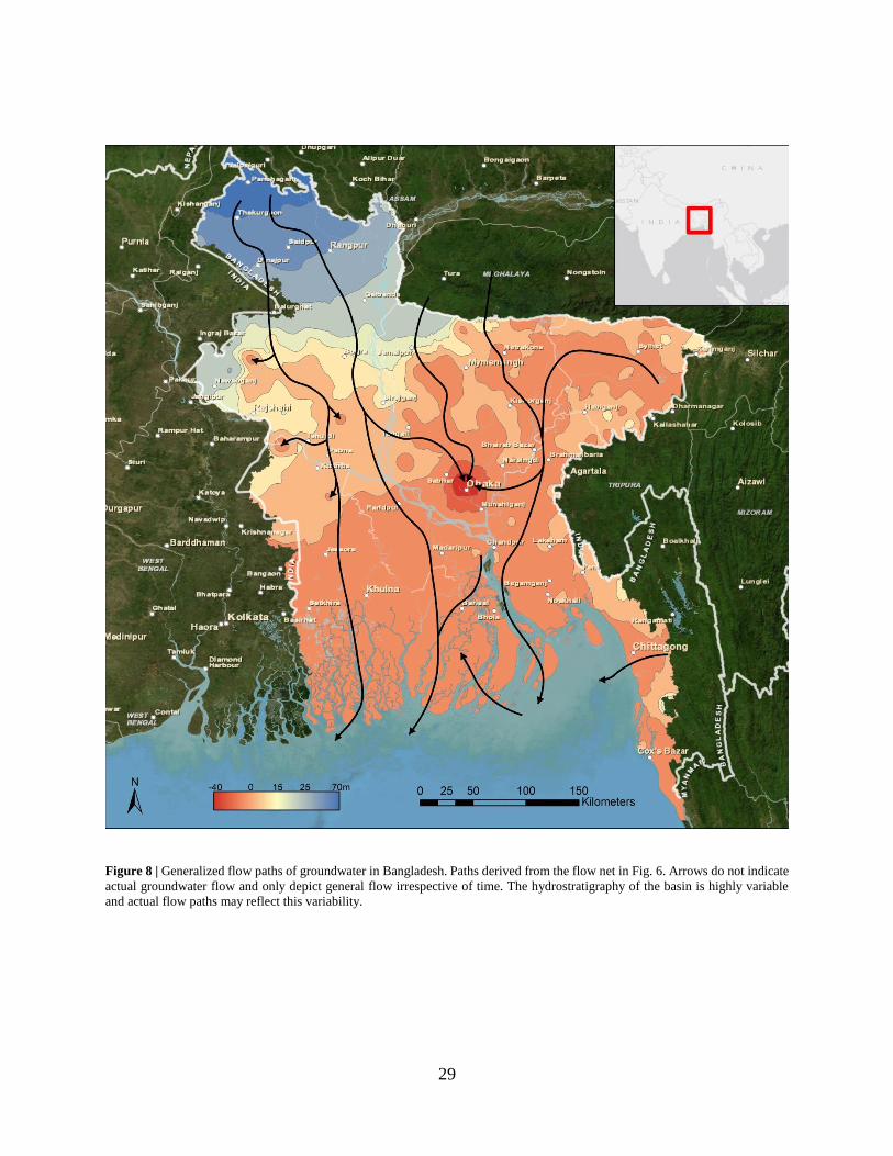
that exist in the central portion of the country. Some flow lines suggest flow from the Bay of
Bengal inland toward the tidal reaches of southwest Bangladesh (Fig. 8). Flow is not entirely sub-
surficial, but dictated by local flow cells with generalized flow toward the southeast.
Water table elevations in the shallow aquifer appear to be falling. Many researchers have
assumed that the shallow aquifer systems were fully replenished during the monsoon season.
Recent studies (Shamsudduha et al., 2011; Shamsudduha et al., 2012) suggest that parts of
Bangladesh – especially the central and northwest – are experiencing declining trends in water
table elevation as a result of dry season irrigation. The most significant cone of depression exists
beneath the city of Dhaka and extends ~50 km across. Dhaka is a megacity (metropolitan
population of 12 million and a growth rate of 3.48% annually; Ibrahim and Kamal, 2012). With
the current large population and rapid growth rate, the need for freshwater can be expected to grow
in-step. In contrast, groundwater elevations in southern Bangladesh are increasing (0.5-4 cm/yr)
as a result in local rises in sea-level (0.4-0.8 cm/yr; (Shamsudduha et al., 2011). Sea level rise may
28
result in changing the hydraulic characteristics of the aquifer system and ultimately shift the
salinity front farther inland.
Groundwater amplitudes provide insight into potential sources of recharge. The high
amplitudes found throughout the central portion of the country, along with two significant zones
east and west of the Jamuna River, are recharged through monsoonal contributions (Fig. 7). The
shallow aquifers in the region dry out throughout the dry season both naturally and through
groundwater abstraction (Harvey et al., 2006; Hoque et al., 2007; Shamsudduha et al., 2009;
Shamsudduha et al., 2011; Shamsudduha et al., 2012). The reason for two distinct regions of high
amplitude may be due to surface recharge from the Jamuna River during the dry season, effectively
dividing the monsoonal recharged system. The reason for lower amplitudes is more difficult to
constrain; however, significant controls must include topography, tides, and hydraulic
conductivity. The northwest region of Bangladesh experiences low groundwater amplitudes due
to more significant topographical gradients (0.4 m/km) and consequently water table gradients.
Water table elevations remain relatively static as these gradients allow continued groundwater
flow, resulting in little accumulation or mounding of groundwater. The southwest and Sylhet Basin
is characterized by very low topographical gradients and subsequently low water table gradients.
Most of the area lies within 3 m of sea level. In the southwest, this may result in tidal modulation
of the groundwater elevations. Furthermore, the coastal zone is characterized by a laterally
extensive and significant (up to 10 m thick) silt confining layer (Umitsu, 1993; Ravenscroft and
McArthur, 2004) (Fig. 9). This upper aquitard inhibits surface recharge. Therefore, in areas with
sufficiently incised (>10 m) tidal channels, more recharge can be expected from the tidal channels.
This may be a control on the observed regionally salinity in the southwest.
29
Figure 8 | Generalized flow paths of groundwater in Bangladesh. Paths derived from the flow net in Fig. 6. Arrows do not indicate
actual groundwater flow and only depict general flow irrespective of time. The hydrostratigraphy of the basin is highly variable
and actual flow paths may reflect this variability.

30
Figure 9 | Generalized aquifer stratigraphy in coastal Bangladesh (Ravenscroft and McArthur, 2004). The upper aquitard results
in limited surface water recharge and likely contributes to regional groundwater salinity issues.
Modeling the Tidal Channel-Aquifer System
We chose to model the aquifer system over a realistic range for each model parameter (TA,
TC, S, TR). The model output (THI distance) provides an indication of how connected the tidal
channels are to the aquifer system. The results suggest that the dominant control on THI distance
is storativity. Confined values of storativity resulted in significant THI distances (>500 m), semi-
confined values resulted in moderate THI distances (~100-300 m), and unconfined values resulted
in small THI distances (~50-100 m). Variability in THI distances suggest that storativity is a
dominant control on tidal channel-aquifer connectivity. Furthermore, for a specific value of
storativity, when other parameters are varied, there is little to no influence on THI distance – with
the exception of aquifer transmissivity.
31
A secondary control on THI distance is aquifer transmissivity. Similar to storativity, THI
distances varied greatly over the range of aquifer transmissivities with high aquifer transmissivity
resulting in the largest THI distances. However, even at high aquifer transmissivities, THI
distances were not as significant as the low storativity scenario. Furthermore, variations in
storativity affect THI distances associated with aquifer transmissivity variations more profoundly
than the converse. For instance, when aquifer transmissivity is high (thick, sandy aquifer) and
storativity is high (unconfined), the THI distance is lower in relation to other high aquifer
transmissivities. This would suggest that storativity exhibits a dominant control on tidal channel-
aquifer system connectivity.
Less significant controls on THI distance are channel transmissivity and tidal range.
However, channel transmissivity exhibits significant control at lower values (silt or clay channels).
This suggests that sufficiently low channel transmissivities dampen tidal channel-aquifer system
interactions, while normal to high channel transmissivities appear to have little effect. Low channel
transmissivities effectively limit pressure exchange between the tidal channel and groundwater
and serve as a limiting factor for the system. Once the transmissivity is sufficiently high, pressure
exchange can continue unimpeded.
Tidal range is the least significant parameter with very little complexity in tidal range
variations. The variations in THI distance from a low tidal range to a high tidal range are fairly
uniform for both the relative and absolute cutoffs. For instance, as tidal range varies from low to
high, there is little to no change in THI distance. Therefore, tidal range as described in this model
has no impact on tidal channel-aquifer system interactions. This may not, however, fully describe
the groundwater-surface water system. Further work may incorporate phase lags between the
32
bounding channels and tidal asymmetries – both of which may influence the measured THI
distance.
The system of monitoring wells and NTSW gauges is not extensive enough to understand
definitive flow patterns or magnitude of flow. Furthermore, water elevation data is very limited in
southwest Bengal, especially in uninhabited regions such as the Sundarbans. Increasing the
network of monitoring wells and surface water gauges can provide a better depiction of local and
regional groundwater flow patterns.
Hydraulic Diffusivity and Regression Analysis
Three of the more complex parametric relationships were chosen and analyzed: 1) S vs. TA,
2) S vs. TC, and 3) TC vs. TA. These parameters were run through the model at a finer resolution
(50x50 opposed to 3x3) and the results were then plotted as a surface where the z-axis was THI
distance (Fig. 10).
The surface plots provide a more complete view of the controls on THI distance; though,
the dominant controls are still primarily storativity and secondarily aquifer transmissivity with
channel transmissivity becoming influential as it approaches zero. THI distances grow rapidly with
a concave-up surface shape as aquifer storativity increases in relation to both aquifer transmissivity
(Fig. 10A) and channel transmissivity (Fig. 10B). This suggests that aquifer storativity becomes
more influential on THI distance at higher values. Conversely, THI distances grow rapidly with a
concave-down surface shape as aquifer transmissivity increases in step with channel transmissivity
(Fig. 10C). This concave-down shape suggests that aquifer transmissivity becomes less influential
on THI distance at higher values. These surface plots corroborate previous notions that aquifer
storativity is the primary control with aquifer transmissivity being the secondary control.

33
Figure 10 | Three dimensional surface plots of THI distances as a function of changes in model parameters. A. aquifer storativity
vs. aquifer transmissivity, B. aquifer storativity vs. channel transmissivity, C. channel transmissivity vs. aquifer transmissivity.
Note the z-axes are not equal.
Furthermore, hydraulic diffusivities (T/S) for both the aquifer (DA) and the channel (DC)
were calculated using model values. A regression of THI distance on the square root of the
calculated diffusivities resulted in Equation 5.
𝑇𝐻𝐼̂ = 4.6119√𝐷𝐴 + 1.8625√𝐷𝐶 + 73.808 (5)
A B
C
34
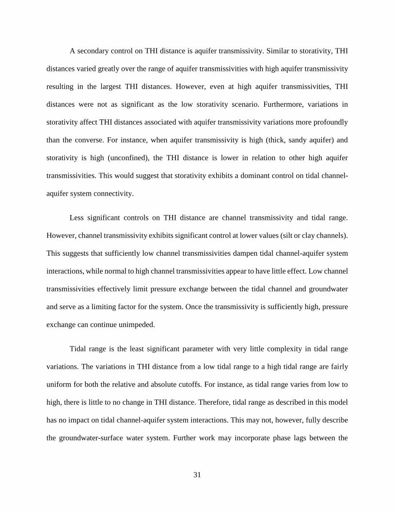
The regression equation of THI distance fits the model data well (r2=0.746) and
corroborates that hydraulic diffusivities are the most significant control on aquifer and surface
water connectivity, with variation in other parameters (TR) having little effect (Fig. 11).
A
B
Figure 11 | Regression analysis of THI distances from the model. A. Regression plane of THI
distance with model values of hydraulic diffusivities plotted in red. B. THI predicated from the
model plotted against THI predicated from the regression. The regression of THI has an r2 of
0.746.
35
Origin of Aquifer Salinity in Southwest Bengal
Aquifer salinity is a significant issue for both irrigation and drinking water uses throughout
coastal Bengal. Many studies (BGS and DPHE, 2001; Ravenscroft and McArthur, 2004; Bhuiyan
and Dutta, 2011; Khan et al., 2011; Rahman and Majumder, 2011) confirm the presence of
brackish groundwater in southwest Bangladesh. Salinity is highly variable in the vertical direction
with most of the shallow aquifer being saline (BGS and DPHE, 2001), though freshwater does
occur in the deeper aquifer (>300 m) and some local lenses. Concentrations of sodium, potassium,
and boron (indicators of overall salinity) are >70 mg/L, >5 mg/L, >0.1 mg/L respectively. The
WHO and the Bangladeshi government recommended guideline for safe levels of sodium in
drinking water is <200 mg/L, of which 8.5% of wells (and nearly all wells in the southwest) exceed
these guidelines (BGS and DPHE, 2001).
Most studies assume a connate origin of the brackish groundwater in the coastal region
based on a study (Hoque et al., 2003) of brackish groundwater origin in Comilla in eastern
Bangladesh. The study suggests that after the LGM, rates of sea level rise exceeded rates of
sediment infill resulting in an estuarine environment in the Bengal Basin and allowing for the
formation of the lower aquitard (Fig. 9). The delta then continued to prograde between 14 and 8
ka. Due to rising sea level and sedimentary infill, conditions were not favorable to flush the
brackish groundwater from the pores. The study acknowledges that intrusion of modern sea water
is not possible due to the distance of Comilla from the Bay of Bengal. However, southwest
Bangladesh is proximally closer to and much more connected (via tidal channel network) with the
Bay of Bengal. As such, a connate origin may not fully explain the observed groundwater salinities
in the southwest.
36
A study (Essink, 2001) in the Netherlands suggests poldering alone can result in aquifer
salinization. The study also suggests that sea level rise is a significant control on groundwater
salinization beneath the polder, though it does acknowledge that the timescale of sea level related
salinization may take upwards of centuries depending on rate of sea level rise, polder proximity to
the sea, and hydrogeological characteristics of the polder. This may suggest a younger origin of
the brackish groundwater in southwest Bengal or at least provide a different framework for
understanding the underlying aquifer relationships with the tidal network. Above, we offer
possible behaviors between these two systems.

37
CHAPTER V
CONCLUSION
The effects of climate change and sea level rise have induced migration in the Bengal Basin
and such movement, along with the associated stress to the human and natural landscapes, can be
expected to increase in the future. Access to freshwater is integral in an individual’s decision to
migrate and thus changes in surface water and groundwater interactions have significant bearing
on human migration in the face of climate change. These changes are amplified by a number of
environmental (e.g. cyclonic activity and storm surge) and anthropogenic controls (e.g. poldering
and aquaculture). The low-lying region of the Bengal Basin remains highly susceptible to sea level
rise through decreased resilience to storm surge, while the widespread occurrence of arsenic and
brackish groundwater further complicate an already stratigraphically complex aquifer system.
Arsenic research has received a bulk of prior research attention; however, determining the origin
of the brackish groundwater may provide significant insights into mitigating water stress in the
future as well. The prevailing hypothesis on the origin of brackish water in the southwest is based
on data from fluvially-dominated eastern Bangladesh. This region experiences different
hydrogeologic controls on surface water and groundwater interactions which may result in
differences in connectivity between the two systems relative to the tidally-dominated southwest.
While southwest Bengal may have experienced a similar evolution throughout the Pleistocene, the
connate origin hypothesis may not fully explain the prevalence of brackish groundwater in the
region. Furthermore, studies of other coastal regions suggest poldering and saline aquaculture may
have an appreciable impact. Predicting and mitigating such changes will require expansion of data
38
and reevaluation of assumptions on surface water and groundwater interactions in southwest
Bengal.
This study reconsiders the underlying assumptions of surface water and groundwater
interactions in southwest Bengal. We found the potential connection of the shallow aquifer system
with the tidal surface network over a variety of hydrogeologic parameters. Furthermore, we found
hydraulic diffusivity to be the dominant control on THI distance and the connection between the
aquifer and surface water systems. Our research shows that tidal surface waters can propagate
inland under favorable hydrogeologic conditions, though further modeling is necessary to
determine the sodium flux into the aquifer.
39
Appendix
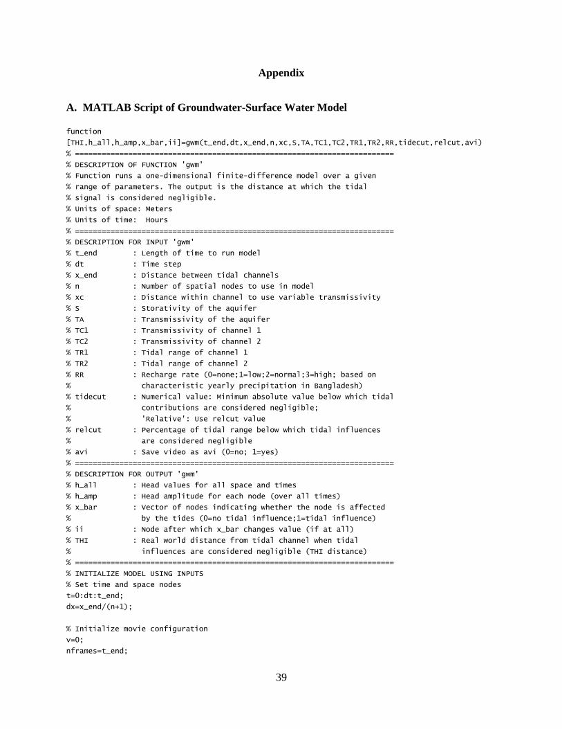
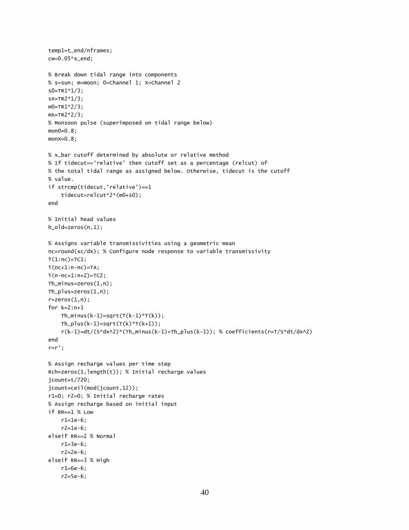
A. MATLAB Script of Groundwater-Surface Water Model
function
[THI,h_all,h_amp,x_bar,ii]=gwm(t_end,dt,x_end,n,xc,S,TA,TC1,TC2,TR1,TR2,RR,tidecut,relcut,avi)
% ========================================================================
% DESCRIPTION OF FUNCTION 'gwm'
% Function runs a one-dimensional finite-difference model over a given
% range of parameters. The output is the distance at which the tidal
% signal is considered negligible.
% Units of space: Meters
% Units of time: Hours
% ========================================================================
% DESCRIPTION FOR INPUT 'gwm'
% t_end : Length of time to run model
% dt : Time step
% x_end : Distance between tidal channels
% n : Number of spatial nodes to use in model
% xc : Distance within channel to use variable transmissivity
% S : Storativity of the aquifer
% TA : Transmissivity of the aquifer
% TC1 : Transmissivity of channel 1
% TC2 : Transmissivity of channel 2
% TR1 : Tidal range of channel 1
% TR2 : Tidal range of channel 2
% RR : Recharge rate (0=none;1=low;2=normal;3=high; based on
% characteristic yearly precipitation in Bangladesh)
% tidecut : Numerical value: Minimum absolute value below which tidal
% contributions are considered negligible;
% 'Relative': Use relcut value
% relcut : Percentage of tidal range below which tidal influences
% are considered negligible
% avi : Save video as avi (0=no; 1=yes)
% ========================================================================
% DESCRIPTION FOR OUTPUT 'gwm'
% h_all : Head values for all space and times
% h_amp : Head amplitude for each node (over all times)
% x_bar : Vector of nodes indicating whether the node is affected
% by the tides (0=no tidal influence;1=tidal influence)
% ii : Node after which x_bar changes value (if at all)
% THI : Real world distance from tidal channel when tidal
% influences are considered negligible (THI distance)
% ========================================================================
% INITIALIZE MODEL USING INPUTS
% Set time and space nodes
t=0:dt:t_end;
dx=x_end/(n+1);
% Initialize movie configuration
v=0;
nframes=t_end;
40
temp1=t_end/nframes;
cw=0.05*x_end;
% Break down tidal range into components
% s=sun; m=moon; 0=Channel 1; X=Channel 2
s0=TR1*1/3;
sX=TR2*1/3;
m0=TR1*2/3;
mX=TR2*2/3;
% Monsoon pulse (superimposed on tidal range below)
mon0=0.8;
monX=0.8;
% x_bar cutoff determined by absolute or relative method
% If tidecut=='relative' then cutoff set as a percentage (relcut) of
% the total tidal range as assigned below. Otherwise, tidecut is the cutoff
% value.
if strcmp(tidecut,'relative')==1
tidecut=relcut*2*(m0+s0);
end
% Initial head values
h_old=zeros(n,1);
% Assigns variable transmissivities using a geometric mean
nc=round(xc/dx); % Configure node response to variable transmissivity
T(1:nc)=TC1;
T(nc+1:n-nc)=TA;
T(n-nc+1:n+2)=TC2;
Th_minus=zeros(1,n);
Th_plus=zeros(1,n);
r=zeros(1,n);
for k=2:n+1
Th_minus(k-1)=sqrt(T(k-1)*T(k));
Th_plus(k-1)=sqrt(T(k)*T(k+1));
r(k-1)=dt/(S*dx^2)*(Th_minus(k-1)+Th_plus(k-1)); % coefficients(r=T/S*dt/dx^2)
end
r=r';
% Assign recharge values per time step
Rch=zeros(1,length(t)); % Initial recharge values
jcount=t/720;
jcount=ceil(mod(jcount,12));
r1=0; r2=0; % Initial recharge rates
% Assign recharge based on initial input
if RR==1 % Low
r1=1e-6;
r2=1e-6;
elseif RR==2 % Normal
r1=3e-6;
r2=2e-6;
elseif RR==3 % High
r1=6e-6;
r2=5e-6;
41
end
% Only assigns recharge for June (6), July (7), Aug (8), Sept (9); All
% other months recharge is zero
jj= jcount==6;
Rch(jj)=r1;
jj= jcount==7;
Rch(jj)=r1;
jj= jcount==8;
Rch(jj)=r2;
jj= jcount==9;
Rch(jj)=r2;
% Head of the tidal channels (Boundary Conditions)
h0=m0*sin(2*pi*t/12.42)+s0*sin(2*pi*t/12)+mon0*sin(2*pi*t/8760+3*pi/4);
hX=mX*sin(2*pi*t/12.42)+sX*sin(2*pi*t/12)+monX*sin(2*pi*t/8760+3*pi/4);
% Construct the finite-difference matrix
m_diag=sparse(1:n,1:n,1+2*r,n,n);
l_diag=sparse(2:n,1:n-1,-r(2:n),n,n);
u_diag=sparse(1:n-1,2:n,-r(1:n-1),n,n);
A=m_diag+l_diag+u_diag;
% Preallocate solution matrix
h_all=zeros(n,length(t));
% ========================================================================
% SOLVE EQUATIONS for length(t) time steps
for j=1:length(t)
R=Rch(j);
I=0; % Irrigation term (set manually)
RHS=h_old+R*dt/S+I*dt/S;
RHS(1)=RHS(1)+r(1)*h0(j);
RHS(n)=RHS(n)+r(n)*hX(j);
h_new=A\RHS;
h_all(:,j)=h_new;
h_old=h_new;
% Make movie if requested
if avi==1
temp2=mod(j,temp1);
if temp2==0
v=v+1;
% Water surface configuration
% Groundwater Heads of all nodes
xplot=0:dx:x_end;
hplot=[h0(j);h_new;hX(j)];
a=plot(xplot,hplot,'b');
hold on
% Tidal Channel 1 heads
xbcplot1=[-cw 0];
hbcplot1=[h0(j) h0(j)];
b=plot(xbcplot1,hbcplot1,'b');
42
% Tidal Channel 2 heads
xbcplot2=[x_end x_end+cw];
hbcplot2=[hX(j) hX(j)];
c=plot(xbcplot2,hbcplot2,'b');
% Channel and land configuration
% Embankment elevation
xbank=[0 x_end];
ybank=[3 3];
d=plot(xbank,ybank,'r:');
% Ground surface elevation
xsurf=[0 x_end];
ysurf=[0.5 0.5];
e=plot(xsurf,ysurf,'k:');
% Channel boundary
xchan1=[0 0];
xchan2=[x_end x_end];
ychan=[-5 5];
f=plot(xchan1,ychan,'k');
g=plot(xchan2,ychan,'k');
hold off
% Axes and legend configuration
xlabel('Island Width (m)')
ylabel('Elevation (m above baselevel)')
axis([-cw x_end+cw -4 4]);
legend([a d e f],{'Groundwater Head','Embankment Surface','Ground Surface','Channel
Boundary'},'Location','SouthEast')
Mov(v) = getframe(gcf);
end
end
end
% Save movie as avi in same directory as script
if avi==1
movie(Mov)
movie2avi(Mov,'GW_Movie','compression','none')
end
% ========================================================================
% FILTER DATA
x_bar=zeros(1,n); % Initial x_bar values
h_amp=zeros(1,n); % Initial h_amp values
for i=1:n
% HIGH-PASS FILTER
% do a low-pass filter to determine monsoonal signal
% subtract the low frequency signal from the data to obtain the tidal
% signal
% DETREND AND TRANSFORM DATA
y = h_all(i,:);
X=length(y);
43
mn=mean(y);
data = y-mn; % Detrend data series by removing mean
delta_t = dt/8760; % Time step associated with data
% CALL LOW-PASS FILTER FUNCTION
cutoff_f = 120/dt;
fdata=lpfilt(data',delta_t,cutoff_f);
fdata=fdata+mn; % add mean back
% FIND HIGH FREQUENCIES
fdata2=y-fdata'; % Subtract low-pass data from original data
% RECORD WHETHER NODES INFLUENCED BY THE TIDES
nOK=round(X/10);
h_amp(i)=max(fdata2(nOK+1:X-nOK))-min(fdata2(nOK+1:X-nOK));
x_bar(i)=0;
if h_amp(i) >= tidecut
x_bar(i)=1;
end
end
% ========================================================================
% FIND THE NODE WHEN TIDES BECOME NEGLIGIBLE
ii=find(diff(x_bar)~=0);
if ~isempty(ii)
THI=ii(1)*dx; % Convert to real world distance from tidal channel
else
THI=x_bar(1)*x_end/2; % Tidal signal extends the length of aquifer
end
end
% ========================================================================
function fdata = lpfilt(data,delta_t,cutoff_f)
% LOW-PASS FILTER
% Peforms low-pass filtering by multiplication in frequency domain using
% a 3-point taper (in frequency space) between pass-band and stop band.
% Coefficients suggested by D. Coats, Battelle, Ventura.
% Written by Chris Sherwood, 1989; revised by P. Wiberg, 2003.
n=length(data);
mn=mean(data);
data=data-mn; %linearly detrend data series
P=fft(data); N=length(P);
filt=ones(N,1);
k=floor(cutoff_f*N*delta_t);
% filt is a tapered box car, symmetric over the 1st and 2nd half of P,
% with 1's for frequencies < cutoff_f and 0's for frequencies > cutoff_f
filt(k+1:k+3)=[0.715 0.24 0.024];
filt(k+4:N-(k+4))=0*filt(k+4:N-(k+4));
filt(N-(k+1:k+3))=[0.715 0.24 0.024];
P=P.*filt;
fdata=real(ifft(P)); %inverse fft of modified data series
fdata=fdata(1:n)+mn; %add mean back into filtered series
end
44
REFERENCES
Acharyya, S.K., Lahiri, S., Raymahashay, B.C., and Bhowmik, A., 2000, Arsenic toxicity of
groundwater in parts of the Bengal basin in India and Bangladesh: the role of Quaternary
stratigraphy and Holocene sea-level fluctuation: Environmental Geology, v. 39, no. 10, p.
1127–1137, doi: 10.1007/s002540000107.
Ahmed, K.M., Bhattacharya, P., Hasan, M.A., Akhter, S.H., Alam, S.M.M., Bhuyian, M.A.H.,
Imam, M.B., Khan, A.A., and Sracek, O., 2004, Arsenic enrichment in groundwater of the
alluvial aquifers in Bangladesh: an overview: Applied Geochemistry, v. 19, no. 2, p. 181–
200, doi: 10.1016/j.apgeochem.2003.09.006.
Alam, M., Alam, M.M., Curray, J.R., Chowdhury, M.L.R., and Gani, M.R., 2003, An overview
of the sedimentary geology of the Bengal Basin in relation to the regional tectonic
framework and basin-fill history: Sedimentary Geology, v. 155, no. 3-4, p. 179–208, doi:
10.1016/S0037-0738(02)00180-X.
Ali, A., 1999, Climate change impacts and adaptation assessment in Bangladesh: Climate
Research, v. 12, p. 109–116.
Ali, A., 1996, Vulnerability of Bangladesh to climate change and sea level rise through tropical
cyclones and storm surges: Water, Air, & Soil Pollution, v. 92, no. 1, p. 171–179.
Azad, A.K., Jensen, K.R., and Lin, C.K., 2009, Coastal Aquaculture Development in
Bangladesh: Unsustainable and Sustainable Experiences: Environmental Management, v.
44, no. 4, p. 800–809, doi: 10.1007/s00267-009-9356-y.
Bahar, M.M., and Reza, M.S., 2010, Hydrochemical characteristics and quality assessment of
shallow groundwater in a coastal area of Southwest Bangladesh: Environmental Earth
Sciences, v. 61, no. 5, p. 1065–1073, doi: 10.1007/s12665-009-0427-4.
Bangladesh Meteorological Department, 2012, Total Rainfall (mm) in Monsoon over Khulna
Division.
Barua, D.K., 1990, Suspended sediment movement in the estuary of the Ganges-Brahmaputra-
Meghna river system: Marine Geology, v. 91, no. 3, p. 243–253, doi: 10.1016/0025-
3227(90)90039-M.
BGS, and DPHE, 2001, Arsenic contamination of groundwater in Bangladesh: British
Geological Survey.
Bhuiyan, M.J.A.N., and Dutta, D., 2011, Control of salt water intrusion due to sea level rise in
the coastal zone of Bangladesh: Coastal Processes II, v. 149, p. 163–173, doi:
10.2495/CP110141.
45
Chowdhury, M.A., Khairun, Y., Salequzzaman, M., and Rahman, M.M., 2011, Effect of
combined shrimp and rice farming on water and soil quality in Bangladesh: Aquaculture
International, v. 19, no. 6, p. 1193–1206, doi: 10.1007/s10499-011-9433-0.
Dasgupta, S., Huq, M., Khan, Z.H., Ahmed, M.M.Z., Mukherjee, N., Khan, M.F., and Pandey,
K., 2010, Vulnerability of Bangladesh to Cyclones in a Changing Climate: Potential
Damages and Adaptation Cost: Environment, , no. April, p. 54.
Esri, I-cubed, USDA, USGS, AEX, GeoEye, Getmapping, Aerogrid, IGN, IGP, UPR-EGP, and
GIS User Community, 2012, Imagery:.
Essink, G.H.P.O., 2001, Salt Water Intrusion in a Three-dimensional Groundwater System in
The Netherlands : A Numerical Study: , p. 137–158.
FAO, 2012, Irrigation in Southern and Eastern Asia in figures: AQUASTAT Survey - 2011:
Food and Agriculture Organization of the United Nations, 1–487 p.
GADM, 2012, Global Administrative Areas:.
Gaus, I., Kinniburgh, D.G., Talbot, J.C., and Webster, R., 2003, Geostatistical analysis of arsenic
concentration in groundwater in Bangladesh using disjunctive kriging: Environmental
Geology, v. 44, no. 8, p. 939–948, doi: 10.1007/s00254-003-0837-7.
Goodbred, S.L., and Kuehl, S.A., 2000a, Enormous Ganges-Brahmaputra sediment discharge
during strengthened early Holocene monsoon: Geology, v. 28, no. 12, p. 1083–1086, doi:
10.1130/0091-7613(2000)28<1083:EGSDDS>2.0.CO;2.
Goodbred, S.L., and Kuehl, S.A., 2000b, The significance of large sediment supply, active
tectonism, and eustasy on margin sequence development: Late Quaternary stratigraphy and
evolution of the Ganges–Brahmaputra delta: Sedimentary Geology, v. 133, no. 3-4, p. 227–
248, doi: 10.1016/S0037-0738(00)00041-5.
Goodbred, S.L., Kuehl, S.A., Steckler, M.S., and Sarker, M.H., 2003, Controls on facies
distribution and stratigraphic preservation in the Ganges–Brahmaputra delta sequence:
Sedimentary Geology, v. 155, no. 3-4, p. 301–316, doi: 10.1016/S0037-0738(02)00184-7.
Harvey, C.F., Ashfaque, K.N., Yu, W., Badruzzaman, A.B.M., Ali, M.A., Oates, P.M., Michael,
H. a., Neumann, R.B., Beckie, R., Islam, S., and Ahmed, M.F., 2006, Groundwater
dynamics and arsenic contamination in Bangladesh: Chemical Geology, v. 228, no. 1-3, p.
112–136, doi: 10.1016/j.chemgeo.2005.11.025.
Harvey, C.F., Swartz, C.H., Badruzzaman, a B.M., Keon-Blute, N., Yu, W., Ali, M.A., Jay, J.,
Beckie, R., Niedan, V., Brabander, D., Oates, P.M., Ashfaque, K.N., Islam, S., Hemond,
H.F., et al., 2002, Arsenic mobility and groundwater extraction in Bangladesh.: Science
(New York, N.Y.), v. 298, no. 5598, p. 1602–6, doi: 10.1126/science.1076978.
46
Hoque, M., Hasan, K., and Ravenscroft, P., 2003, Investigation of Groundwater Salinity and Gas
Problems in Southeast Bangladesh, in Rahman, A.A. and Ravenscroft, P. eds., Groundwater
Resources and Development in Bangladesh, The University Press Limited, Dhaka,
Bangladesh, p. 373–390.
Hoque, M. a., Hoque, M.M., and Ahmed, K.M., 2007, Declining groundwater level and aquifer
dewatering in Dhaka metropolitan area, Bangladesh: causes and quantification:
Hydrogeology Journal, v. 15, no. 8, p. 1523–1534, doi: 10.1007/s10040-007-0226-5.
IPCC, 2007, Climate Change 2007: Impacts, Adaptation, and Vulnerability. Contribution of
Working Group III to the Fourth Assessment Report of the Intergovernmental Panel on
Climate Change. (M. L. Parry, O. F. Canziani, J. P. Palutikof, P. J. van der Linden, & C. E.
Hanson, Eds.): Cambridge University Press, Cambridge, UK.
IPCC, 2012, Managing the Risks of Extreme Events and Disasters to Advance Climate Change
Adaptation. A Special Report of Working Groups I and II of the Intergovernmental Panel
on Climate Change (C. B. Field, V. Barros, T. F. Stockner, D. Qin, D. J. Dokken, K. L. Ebi,
M. D. Mastrandrea, K. J. Mach, G.-K. Plattner, S. K. Allen, M. Tignor, & P. M. Midgley,
Eds.): Cambridge University Press, Cambridge, UK.
Islam, M.R., Begum, S.F., Yamaguchi, Y., and Ogawa, K., 1999, The Ganges and Brahmaputra
rivers in Bangladesh: basin denudation and sedimentation: Hydrological Processes, v. 13,
no. 17, p. 2907–2923, doi: 10.1002/(SICI)1099-1085(19991215)13:17<2907::AID-
HYP906>3.0.CO;2-E.
Karim, M.R., 2010, Assessment of rainwater harvesting for drinking water supply in
Bangladesh: Water Science & Technology: Water Supply, v. 10, no. 2, p. 243, doi:
10.2166/ws.2010.896.
Kartiki, K., 2011, Climate change and migration: a case study from rural Bangladesh: Gender &
Development, v. 19, no. 1, p. 23–38, doi: 10.1080/13552074.2011.554017.
Khan, A., Ireson, A., and Kovats, S., 2011, Drinking Water Salinity and Maternal Health in
Coastal Bangladesh: Implications of Climate Change: Environmental health …, v. 119, no.
9, p. 1328–1332.
Kinniburgh, D.G., and Kosmus, W., 2002, Arsenic contamination in groundwater: some
analytical considerations.: Talanta, v. 58, no. 1, p. 165–80.
Kuehl, S.A., Allison, M.A., Goodbred, S.L., and Kudrass, H., 2005, River Deltas: Concepts,
Models, and Examples, in Giosan, L. and Bhattacharya, J.P. eds., Holocene, SEPM (Society
for Sedimentary Geology), p. 413–434.
Lehner, B., Verdin, K., and Jarvis, A., 2008, New Global Hydrography Derived From
Spaceborne Elevation Data: Eos, Transactions American Geophysical Union, v. 89, no. 10,
p. 93, doi: 10.1029/2008EO100001.

47
McArthur, J.M., Nath, B., Banerjee, D.M., Purohit, R., and Grassineau, N., 2011, Palaeosol
Control on Groundwater Flow and Pollutant Distribution: The Example of Arsenic.:
Environmental Science & Technology, v. 45, p. 1376–1383, doi: 10.1021/es1032376.
McArthur, J.M., Ravenscroft, P., Banerjee, D.M., Milsom, J., Hudson-Edwards, K. a., Sengupta,
S., Bristow, C., Sarkar, A., Tonkin, S., and Purohit, R., 2008, How paleosols influence
groundwater flow and arsenic pollution: A model from the Bengal Basin and its worldwide
implication: Water Resources Research, v. 44, no. W11411, doi: 10.1029/2007WR006552.
Meehl, G.A., Stocker, T.F., Collins, W.D., Friedlingstein, P., Gaye, A.T., Gregory, J.M., Kitoh,
A., Knutti, R., Murphy, J.M., A. Noda, S.C.B.R., Watterson, I.G., Weaver, A.J., and Zhao,
Z.-C., 2007, Global Climate Projections, in Solomon, S., Qin, D., Manning, M., Chen, Z.,
Marquis, M., Averyt, K.B., Tignor, M., and Miller, H.L. eds., Climate Change 2007: The
Physical Science Basis. Contribution of Working Group I to the Fourth Assessment Report
of the Intergovernmental Panel on Climate Change, Cambridge University Press,
Cambridge, UK, p. 747–845.
Mehedi, H., 2010, Climate induced displacement: case study of cyclone Aila in the southwest
coastal region of Bangladesh:, 37 p.
Michael, H.A., and Voss, C.I., 2008, Evaluation of the sustainability of deep groundwater as an
arsenic-safe resource in the Bengal Basin.: Proceedings of the National Academy of
Sciences of the United States of America, v. 105, no. 25, p. 8531–6, doi:
10.1073/pnas.0710477105.
Mondal, M.K., Bhuiyan, S.I., and Franco, D.T., 2001, Soil salinity reduction and prediction of
salt dynamics in the coastal ricelands of Bangladesh: Agricultural Water Management, v.
47, no. 1, p. 9–23, doi: 10.1016/S0378-3774(00)00098-6.
Morgan, J.P., and McIntire, W.G., 1959, Quaternary Geology of the Bengal Basin, East Pakistan
and India: Geological Society of America Bulletin, v. 70, no. 3, p. 319, doi: 10.1130/0016-
7606(1959)70[319:QGOTBB]2.0.CO;2.
National Research Council, 2010, Advancing the Science of Climate Change: The National
Academies Press, Washington, D.C.
Nicholls, R.J., and Cazenave, A., 2010, Sea-level rise and its impact on coastal zones.: Science
(New York, N.Y.), v. 328, no. 5985, p. 1517–20, doi: 10.1126/science.1185782.
Nicholls, R.J., Wong, P.P., Burkett, V., Codignotto, J., Hay, J., McLean, R., Ragoonaden, S.,
Woodroffe, C.D., Abuodha, P.A.O., Arblaster, J., Brown, B., Forbes, D., Hall, J., Kovats,
S., et al., 2007, Coastal systems and low-lying areas, in Climate change 2007: impacts,
adaptation and vulnerability. Contribution of Working Group II to the fourth assessment
report of the Intergovernmental Panel on Climate Change, Cambridge University Press,
Cambridge, UK, p. 315–356.
48
Persits, F.M., Wandrey, C.J., Milici, R.C., and Manwar, A., 2001, U.S. Geological Survey Open
File Report 97-470H:.
Primavera, J.H., 1997, Socio-economic impacts of shrimp culture: Aquaculture Research, v. 28,
no. 10, p. 815–827, doi: 10.1046/j.1365-2109.1997.00946.x.
Rahman, M., and Majumder, R., 2011, Sources of deep groundwater salinity in the southwestern
zone of Bangladesh: Environmental Earth …, v. 63, p. 363–373.
Ravenscroft, P., Burgess, W.G., Ahmed, K.M., Burren, M., and Perrin, J., 2005, Arsenic in
groundwater of the Bengal Basin, Bangladesh: Distribution, field relations, and
hydrogeological setting: Hydrogeology Journal, v. 13, no. 5-6, p. 727–751, doi:
10.1007/s10040-003-0314-0.
Ravenscroft, P., and McArthur, J.., 2004, Mechanism of regional enrichment of groundwater by
boron: the examples of Bangladesh and Michigan, USA: Applied Geochemistry, v. 19, no.
9, p. 1413–1430, doi: 10.1016/j.apgeochem.2003.10.014.
Shamsudduha, M., Chandler, R.E., Taylor, R.G., and Ahmed, K.M., 2009, Recent trends in
groundwater levels in a highly seasonal hydrological system: the Ganges-Brahmaputra-
Meghna Delta: Hydrology and Earth System Sciences Discussions, v. 6, no. 3, p. 4125–
4154, doi: 10.5194/hessd-6-4125-2009.
Shamsudduha, M., Taylor, R.G., Ahmed, K.M., and Zahid, A., 2011, The impact of intensive
groundwater abstraction on recharge to a shallow regional aquifer system: evidence from
Bangladesh: Hydrogeology Journal, v. 19, no. 4, p. 901–916, doi: 10.1007/s10040-011-
0723-4.
Shamsudduha, M., Taylor, R.G., and Longuevergne, L., 2012, Monitoring groundwater storage
changes in the highly seasonal humid tropics: Validation of GRACE measurements in the
Bengal Basin: Water Resources Research, v. 48, no. 2, p. 1–12, doi:
10.1029/2011WR010993.
Thornton, C., Shanahan, M., and Williams, J., 2003, From Wetlands to Wastelands: Impacts of
Shrimp Farming: The Society of Wetland Scientists Bulletin, v. 20, no. 1, p. 48–53, doi:
10.1672/0732-9393(2003)020[0048:FWTWIO]2.0.CO;2.
Umitsu, M., 1993, Late quaternary sedimentary environments and landforms in the Ganges
Delta: Sedimentary Geology, v. 83, no. 3-4, p. 177–186, doi: 10.1016/0037-0738(93)90011-
S.
United Nations, 2010, Cyclone Aila: Joint UN Multi-Sector Assessment & Response
Framework:, 44 p.
United Nations, 2007, Cyclone Sidr: United Nations Rapid Initial Assessment Report:, 1–14 p.

49
Vengosh, A., 2003, Salinization and Saline Environments, in Treatise on Geochemistry Vol. 9:
Environmental Geochemistry, Elsevier, p. 333–365.
WARPO, 2001, National Water Management Plan:, 1–227 p.