group theory and representation theory
TRANSCRIPT

Group Theory and Representation Theory(Lecture Notes, Perpetually in progress)
March 3, 2016
Professor Konstantinos Sfetsos
Department of Nuclear and Particle Physics,Faculty of Physics,
National and Kapodistrian University of Athens,15771 Athens, Greece, Greece
Overview
This course introduces the theory of group representations as the systematic way ofclassifying objects on which a group can act. Furthermore, it reveals how this leadsto a deeper understanding of symmetry aspects of physical systems and how one canuse it to simplify mathematical computations.

Prof. K. Sfetsos LECTURE NOTES ON GROUP REPRESENTATION THEORY
Contents
1 Motivation 4
2 Extended review of Group Theory 5
2.1 Basic definitions . . . . . . . . . . . . . . . . . . . . . . . . . . . . . . . . . 5
2.2 Some examples of groups . . . . . . . . . . . . . . . . . . . . . . . . . . . 6
2.2.1 Abelian groups . . . . . . . . . . . . . . . . . . . . . . . . . . . . . 6
2.2.2 Non-Abelian groups . . . . . . . . . . . . . . . . . . . . . . . . . . 6
2.3 More theorems and definitions . . . . . . . . . . . . . . . . . . . . . . . . 8
2.3.1 Subgroups . . . . . . . . . . . . . . . . . . . . . . . . . . . . . . . . 8
2.3.2 Cyclic groups . . . . . . . . . . . . . . . . . . . . . . . . . . . . . . 9
2.3.3 Generators of a group . . . . . . . . . . . . . . . . . . . . . . . . . 9
2.4 Cosets . . . . . . . . . . . . . . . . . . . . . . . . . . . . . . . . . . . . . . . 10
2.5 Conjugate elements and class structure . . . . . . . . . . . . . . . . . . . 12
2.5.1 Class decomposition . . . . . . . . . . . . . . . . . . . . . . . . . . 12
2.5.2 Distinct elements in a class . . . . . . . . . . . . . . . . . . . . . . 13
2.6 Invariant (or normal) subgroups and factor groups . . . . . . . . . . . . . 15
2.7 Isomorphism and Homomorphism . . . . . . . . . . . . . . . . . . . . . . 17
2.8 Class multiplication . . . . . . . . . . . . . . . . . . . . . . . . . . . . . . . 19
2.8.1 Product of classes . . . . . . . . . . . . . . . . . . . . . . . . . . . . 20
3 Foundations of Group Theory Representations 22
3.1 Reducible and Irreducible Representations . . . . . . . . . . . . . . . . . 23
3.2 Criteria for (ir)reducibility of a representation; Schur’s lemmas . . . . . . 26
3.3 The great orthogonality theorem . . . . . . . . . . . . . . . . . . . . . . . 28
3.4 The character of a representation . . . . . . . . . . . . . . . . . . . . . . . 31
3.5 Decomposition of reducible representations . . . . . . . . . . . . . . . . . 33
3.6 The regular representation . . . . . . . . . . . . . . . . . . . . . . . . . . . 34
3.7 The celebrated theorem . . . . . . . . . . . . . . . . . . . . . . . . . . . . . 35
3.8 Character tables . . . . . . . . . . . . . . . . . . . . . . . . . . . . . . . . . 36
1

Prof. K. Sfetsos LECTURE NOTES ON GROUP REPRESENTATION THEORY
3.8.1 The rules for constructing character tables . . . . . . . . . . . . . 36
3.8.2 Example of character table construction . . . . . . . . . . . . . . . 37
4 Direct product groups 40
4.1 The direct (or Kronecker) product of matrices . . . . . . . . . . . . . . . . 41
4.2 Direct product representations of different groups . . . . . . . . . . . . . 43
4.2.1 Example of character table for direct product representations . . 44
4.3 Direct product representations within the same group . . . . . . . . . . . 45
5 Applications of representation theory 47
5.1 Transformation operators . . . . . . . . . . . . . . . . . . . . . . . . . . . 47
5.2 Constructing representations . . . . . . . . . . . . . . . . . . . . . . . . . 48
5.3 Basis functions for irreducible representations . . . . . . . . . . . . . . . 50
5.3.1 An example . . . . . . . . . . . . . . . . . . . . . . . . . . . . . . . 52
5.4 Representations of Abelian groups . . . . . . . . . . . . . . . . . . . . . . 55
5.4.1 Cyclic groups . . . . . . . . . . . . . . . . . . . . . . . . . . . . . . 55
5.4.2 Bloch’s theorem . . . . . . . . . . . . . . . . . . . . . . . . . . . . . 55
5.4.3 The 2-dim rotation group SO(2) . . . . . . . . . . . . . . . . . . . 56
5.4.4 The Orthogonal group O(2) . . . . . . . . . . . . . . . . . . . . . . 58
5.5 Selection rules . . . . . . . . . . . . . . . . . . . . . . . . . . . . . . . . . . 59
6 The 3-dim rotation group 62
6.1 General rotations . . . . . . . . . . . . . . . . . . . . . . . . . . . . . . . . 62
6.2 Group generators; reps in terms of differential operators . . . . . . . . . 63
6.3 Elements of Lie-algebras . . . . . . . . . . . . . . . . . . . . . . . . . . . . 65
7 SU(2): The group of 2× 2 unitary matrices 68
7.1 Homomorphism between SO(3) with SU(2) . . . . . . . . . . . . . . . . 70
7.2 Representations of SU(2) . . . . . . . . . . . . . . . . . . . . . . . . . . . 71
7.3 The characters . . . . . . . . . . . . . . . . . . . . . . . . . . . . . . . . . . 74
7.3.1 Character decomposition . . . . . . . . . . . . . . . . . . . . . . . 76
7.3.2 The great orthogonality theorem for SU(2) irreps . . . . . . . . . 77
2
Prof. K. Sfetsos LECTURE NOTES ON GROUP REPRESENTATION THEORY
7.4 The Wigner or Clebsch–Gordan coefficients . . . . . . . . . . . . . . . . . 78
7.4.1 Wigner 3− j symbols . . . . . . . . . . . . . . . . . . . . . . . . . . 81
7.5 Tensors operators . . . . . . . . . . . . . . . . . . . . . . . . . . . . . . . . 82
7.5.1 Scalars . . . . . . . . . . . . . . . . . . . . . . . . . . . . . . . . . . 82
7.5.2 Vectors . . . . . . . . . . . . . . . . . . . . . . . . . . . . . . . . . . 82
7.5.3 General tensors . . . . . . . . . . . . . . . . . . . . . . . . . . . . . 82
7.6 The Wigner–Eckart theorem . . . . . . . . . . . . . . . . . . . . . . . . . . 85
7.6.1 Example of tensor decomposition . . . . . . . . . . . . . . . . . . 86
3

Prof. K. Sfetsos LECTURE NOTES ON GROUP REPRESENTATION THEORY
1 Motivation
The common theme of many branches of Mathematical and Physical sciences is sym-
metry. In this module we will learn the principles and mathematical techniques to
exploit symmetry properties of a system. There are two major reasons for doing so: (i)
from a practical view point, reduce significantly or organize better the computational
tasks involved and (ii) at a more conceptual level, provide a fundamental starting
point or classification scheme for a deeper understanding of the system that may lead
to further generalizations and advancements.
What we need is a formalism which will tell us how to extract the maximum informa-
tion from symmetries systematically and avoiding as much as possible the complexi-
ties of the problem at hand. Such a formalism has been developed and referred to as
Group Theory. This module introduces the theory of Group Representations as the sys-
tematic way of classifying objects on which a group can act. Furthermore, it reveals
how this leads to a deeper understanding of symmetry aspects of physical systems
that how one can use it to simplify mathematical computations.
At the end of the module a student should:
• Have a firm understanding of the concepts, theorems and techniques of group rep-
resentation theory.
• Have a clear understanding how to construct irreducible representations of groups.
• Be able to explicitly apply the above to small order groups.
•Have a true appreciation of the importance of the knowledge that they have acquired
and its wide range of applications in mathematical and physical sciences.
Abbreviations
• l.h.s. (r.h.s.) : left (right) hand side
• w.r.t. : with respect to
• i.e. : "in a sense" or "in other words".
• n-dim : n-dimensional.
• rep(s) : representation(s)
• irrep(s) : irreducible representation(s)
4

Prof. K. Sfetsos LECTURE NOTES ON GROUP REPRESENTATION THEORY
2 Extended review of Group Theory
To make these notes self-contained we will provide in this section a rather detailed
and extended review of group theory with emphasis on discrete groups.
2.1 Basic definitions
By a group G we mean a set of objects or operators (called the Group Elements) (a, b, . . . )
which possess the following properties:
1. A composition law or "multiplication"
A · B = AB (for simplicity) , A, B ∈ G , (2.1)
which is associative
(AB)C = A(BC) , ∀ A, B, C ∈ G (2.2)
and closed
AB = C , C ∈ G , ∀ A, B ∈ G . (2.3)
2. There is an element e called the identity or unit element, such that
EA = AE = A , ∀A ∈ G . (2.4)
3. Every element A ∈ G possesses an inverse A−1 such that
A−1A = AA−1 = E , ∀A ∈ G . (2.5)
Remarks:
• This compositions law need not be commutative, that is, generically, AB 6= BA. A
group with a commutative composition law is called Abelian. In all other cases is
called non-Abelian.
• A group contains only one unit element (Exercise).
• The inverse of the inverse of A ∈ G is A itself, that is (A−1)−1 = A (Exercise).
5

Prof. K. Sfetsos LECTURE NOTES ON GROUP REPRESENTATION THEORY
• For each A ∈ G there is a unique inverse (Exercise).
• A group is called finite ( infinite) if the number of its elements is finite (infinite). For
finite groups the number of elements is called order of the group.
2.2 Some examples of groups
2.2.1 Abelian groups
1. The set of all integers constitutes an Abelian infinite group, if the composition law
is the usual addition. The unit element is zero and the inverse of an integer A is −A.
2. Similar to the above example, the set of vectors of a linear n-dim space form an
infinite Abelian group if the composition law is the usual addition of vectors.
3. The set of all rational numbers of the formpq
excluding zero constitutes an Abelian
infinite group, if the composition law is the usual multiplication. The unit element is
one and the inverse ofpq
is justqp
. Unlike, the negative rational numbers, the positive
ones form a group by themselves.
2.2.2 Non-Abelian groups
1. The set of all non-singular n × n matrices over C comprises the General Linear
Group GL(n) under the usual multiplication of matrices, with the unit element the
identity matrix. The group is obviously non-Abelian and infinite dimensional. The
elements of GL(n) depend on 2n2 continuous real parameters and therefore the group
is called continuous.
2. The covering operations of a symmetric object form a group. A covering operation
is a rotation, a reflection or an inversion that sends the object into itself, that is to a
form that is indistinguishable optically from the original one. An important example
of a finite covering group is the covering group of the equilateral triangle (D3), which
will be used extensively in these notes to illustrate various points.
6

Prof. K. Sfetsos LECTURE NOTES ON GROUP REPRESENTATION THEORY
A
B C
y
x
Figure 1: Equilateral triangleand its symmetry axes.
E : Identity operation
A, B, C : Rotations by π about the axes shown
D : Rotation by − 2π
3in z axis(clockwise)
F : Rotation by +2π
3in z axis(anti− clockwise)
(z points outwards)
By inspection one constructs the following Group Multiplication Table (column opera-
tion performed first)E A B C D F
E E A B C D FA A E D F B CB B F E D C AC C D F E A BD D C A B F EF F B C A E D .
(2.6)
For this group we will use the notation D3.
Remarks:
• The group is non-Abelian, since, for instance, AB = D 6= BA = F. Its order h = 6.
• The covering operations may be represented as 2-dim matrices
E =
(1 00 1
),
A =
(1 00 −1
), B =
(−1
2
√3
2√3
212
), C =
(−1
2 −√
32
−√
32
12
), (2.7)
D =
(−1
2
√3
2
−√
32 −1
2
), F =
(−1
2 −√
32√
32 −1
2
).
These matrices act on the 2-dim vector
(xy
). One can readily verify that indeed they
reproduce the table (2.6) (Exercise).
•One may view this group on its own and simply say that it isomorphic to the covering
7

Prof. K. Sfetsos LECTURE NOTES ON GROUP REPRESENTATION THEORY
group of the equilateral triangle.
2.3 More theorems and definitions
Rearrangement Theorem: In a group multiplication table each column or row con-
tains each group element once and only once. This implies that if
G = X1, X2, . . . , Xh , (2.8)
then the set
GXk = X1Xk, X2Xk, . . . , XhXk = G , ∀ Xk ∈ G . (2.9)
2.3.1 Subgroups
Any subset of group elements which itself forms a group G with the same composition
law is called a subgroup H of G. The remaining elements of G cannot form a group
since they do not contain the identity.
Any group has at least two subgroups, the group itself and the group consisting only
of the identity element. Such subgroups are called improper subgroups or trivial sub-
groups. All other subgroups are called proper subgroups.
The covering group of the equilateral triangle has four proper subgroups: E, A,E, B, E, C and E, D, F. The first three are covering groups of three isosceles
triangles.
Exercise: Compute the multiplication table of the covering group of a square (D4)
using the following table and notation:
A
B
C D
Figure 2: Square and its symme-try axes.
E : Identity operation
A, B, C, D : Rotations about axis A, B, C, D
F, G, H : Clockwise rotations byπ
2, π,
3π
2
8

Prof. K. Sfetsos LECTURE NOTES ON GROUP REPRESENTATION THEORY
Find its proper subgroups and indicate the ones that correspond to covering groups
of rectangles.
2.3.2 Cyclic groups
Consider a finite group G. For any X ∈ G consider the sequence
E , Xk , k = 1, 2, . . . . (2.10)
By closure all element in this sequence belong in G and therefore there is a certain
power, say Xn for which Xn = Xm, with m < n. Indeed, unless Xn = E, we have
that the group element Xn−1 = Xm−1 would have appeared earlier in the sequence,
in contrast with our hypothesis. Hence, the elements that appear in the sequence are
distinct up to order n− 1. The integer n is called the order of the element X since it is
the smallest integer for which Xn = E. The sequence
E , X , X2 , . . . , Xn−1 . (2.11)
is called the period of the element X and forms a group (note that X−1 = Xn−1).
This procedure might not exhaust all elements of the group G we started with.
Definition: A group formed entirely of powers of a single element is called cyclic.
Remarks:
• Since XnXm = XmXn, all cyclic groups are Abelian.
• The covering group of the equilateral triangle has three cyclic subgroups of order 2
and one of order 3 (Exercise).
2.3.3 Generators of a group
Definition: The elements Xi, i = 1, 2, . . . , k of a group G are called generators or gen-
erating elements if every X ∈ G can be expressed as a finite product of positive and
negative powers of the Xi’s. The set of relations
gm(X1, X2, . . . , Xk) = E , m = 1, 2, . . . , (2.12)
9

Prof. K. Sfetsos LECTURE NOTES ON GROUP REPRESENTATION THEORY
which are sufficient to determine the entire multiplication table of G are called defining
relations or generating relations of G.
Remarks:
• The sets of generators and defining relations are by no means unique.
• There is always a minimum set of generators without which one cannot generate the
group. It is often practical to use an overdetermined set instead of the minimal one.
Exercise: For the covering group of the equilateral triangle a set of generators is
A, D and the corresponding defining relations are
A2 = E , D3 = E , ADAD−2 = E . (2.13)
2.4 Cosets
Let H = S1 = E, S2, . . . , Sg be a subgroup of order g of a larger group G = X1 =
E, X2, . . . , Xh of order h.
Definition: We call the set of g elements
HXk = S1Xk, S2Xk, . . . , SgXk , Xk /∈ H , (2.14)
the right coset of H with respect to Xk. There is similar definition for the left coset.
Remarks:
• The coset is not a group itself since it does not contain the identity (Exercise).
• The coset HXk has no common elements with H (Exercise).
• The element Xk is called a coset representative and is by no means special. Any ele-
ment of the coset may serve as such a representative.
Proof: If we choose an element A ∈ HXk, then this is of the form A = SmXk. Then
the coset HA = HSmXk = HXk is the same as the original one by the rearrangement
theorem.
• The right (or the left) cosets of the subgroup H are either identical or have no ele-
ments in common.
Proof: Consider the two right cosets HXm and HXn. Assuming that they have one
element in common we have a relation of the form SrXm = SsXn, which implies that
10

Prof. K. Sfetsos LECTURE NOTES ON GROUP REPRESENTATION THEORY
XmX−1n ∈ H. Then by the rearrangement theorem HXmX−1
n = H or HXm = HXn that
is the two cosets are completely identical. A similar proof holds for left cosets as well.
• The order g of the subgroup H is an integral divisor of the order h of the group G.
The integer
` =hg
, (2.15)
is called the index of the subgroup H.
Proof: There are h− g group elements that do not belong to H which we denote by
Xg+1, Xg+2, . . . , Xh. Hence we may construct the following sets of g elements each
H , HXg+1 , HXg+2 , . . . , HXh . (2.16)
Due to the above, no coset has any element in common with H and also the cosets
themselves are either identical or have no common elements as well. Hence, after
keeping only the distinct cosets we have the sets
HX1 , HX2 , . . . , HX` , X1 ≡ E , (2.17)
where ` is a positive integer. Each of these sets has g elements none of them in com-
mon. Hence an element of G should appear in the above sequence only once. There-
fore h = `g.
• In this way we see that we can expand the group G in terms of the right cosets of
any subgroup H as
G =⋃k=1
HXk , X1 ≡ E , (2.18)
with a similar expression for the expansion in terms of the left coset.
• Finite groups whose order h is a prime integer are cyclic Abelian groups.
Proof: If this was not the case the period of some element would have been a subgroup
whose order is a divisor of a prime number. Therefore for each prime there is only one
distinct group, i.e. only one distinct multiplication table.
Exercise: For the covering group of the equilateral triangle choose the subgroup H =
E, A, construct all the right and left cosets and verify the above statements. Repeat
the exercise for the square and choose the subgroup H appropriately.
11

Prof. K. Sfetsos LECTURE NOTES ON GROUP REPRESENTATION THEORY
2.5 Conjugate elements and class structure
Definition: Let A, B ∈ G. They are said to be conjugate elements if there is X ∈ G such
that B = XAX−1.
Remarks:
• One easily shows that if two elements are conjugate to a third element, then they are
conjugate to each other as well (Exercise).
• All mutually conjugate elements can be collected into a class. The class that includes
an element Ai is formed by considering the sequence Xk AiX−1k , k = 1, 2, . . . , h. Of
course some elements may occur more than once in this sequence.
• The unit element forms a class on its own. This class is the only one that is also a
subgroup of G (Exercise).
• All elements of a given class have the same period. Indeed, if An = E we have that
(XAX−1)n = · · · = XAnX−1 = E.
• In Abelian groups every element is a class by itself.
2.5.1 Class decomposition
The various distinct classes of conjugate elements are mutually exclusive.
Proof: Assuming two classes A and B have one element in common then for some
X, Y ∈ G we have that
XArX−1 = YBsY−1 =⇒ CArC−1 = ZBsZ−1 , Z = CX−1Y , ∀ C ∈ G . (2.19)
By ranging over all elements C ∈ G, the l.h.s. generates the entire class A. Similarly
by the rearrangement theorem Z runs over all elements of G and generates the entire
class B. Hence, the two classes must be identical.
Hence, we have the decomposition of G into classes as
G =k⋃
a=1
Ca . (2.20)
12

Prof. K. Sfetsos LECTURE NOTES ON GROUP REPRESENTATION THEORY
Consequently, if ha is the number of elements in the class Ca, we have that
h =k
∑a=1
ha . (2.21)
Exercise: For the equilateral triangle show that the class decomposition leads to
D3 = C1 ∪ C2 ∪ C3 , C1 = E , C2 = A, B, C , C3 = D, F . (2.22)
Exercise: Repeat the previous exercise for D4, the symmetry group of the square and
show that D4 = ∪5a=1Ca, where
C1 = E , C2 = A, B , C3 = C, D , C4 = G , C5 = F, H . (2.23)
2.5.2 Distinct elements in a class
How many distinct elements are there in the class generated by A ∈ G? To answer
this question we define the normalizer:
Definition: The set of elements of G that commute with a fixed element A ∈ G is
called the normalizer of A.1 Remarks:
• The elements of the normalizer form a subgroup NA of G.
Proof: Let Ni ∈ NA, i = 1, 2 arbitrary elements obeying [A, Ni] = 0.2 We easily
establish that
[A, N1N2] = N1[A, N2] + [A, N1]N2 = 0 , [A, N−1i ] = 0 , i = 1, 2 . (2.28)
1More generally let H ⊆ G. Then the normalizer of H in G is
NG(H) = g ∈ G | Hg = gH , (2.24)
Also the centralizer isCG(H) = g ∈ G | hg = gh , ∀ h ∈ H , (2.25)
Obviously, CG(H) ⊆ NG(H). In our case we use the term normalizer and centralizer indistinguishablysince the group element A is fixed, i.e. the subgroup H consists of only one element, that is H = A.
2We will use the notation[A, B] = AB− BA , (2.26)
for any two operators A and B. This is commonly known as the commutator of A and B. Two basicproperties are
[A, B] = −[B, A] , [A, BC] = B[A, C] + [A, B]C . (2.27)
13

Prof. K. Sfetsos LECTURE NOTES ON GROUP REPRESENTATION THEORY
Since, also [A, E] = 0 and by definition associativity is obeyed, the assertion is proved.
•We may expand G into left cosets with respect to NA as
G =`A⋃
k=1
XkNA , X1 ≡ E , (2.29)
where `A = h/nA is the index of NA and nA its order. A typical element of XkNA is
XkN, where N ∈ NA and obeys (XkN)A(XkN)−1 = Xk AX−1k , independent of which
element N is chosen. Hence, all elements belonging to the same coset transform A
in the same manner. Moreover, if we pick up two elements of different cosets, i.e.
Xi 6= Xj, we have that (XiNA)A(XiNA)−1 6= (XjNA)A(XjNA)
−1.
Proof: Assume instead equality. Then easily [A, X−1i Xj] = 0, which means that
X−1i Xj ∈ NA. Then by the rearrangement theorem X−1
i XjNA = NA or XiNA = XjNA,
which contradicts our hypothesis.
Therefore elements of two different cosets of the normalizer NA lead to different trans-
formations. Hence, the number of distinct conjugates of A is the index `A = h/nA of
the normalizer of A. These elements are obtained by applying the transformation
XAX−1, ∀ X ∈ G, but we have just demonstrated that only a number of them, equal
to the index of the normalized `A, are the distinct ones. They can be written as
Xi AX−1i , i = 1, 2, . . . , `A . (2.30)
Exercise: For the covering group of the equilateral triangle show that the normalizers
corresponding to the various elements are
NE = E, A, B, C, D, F , nE = 6 , `E = 1 ,
NA = E, A , nA = 2 , `A = 3 ,
NB = E, B , nB = 2 , `B = 3 , (2.31)
NC = E, C , nC = 2 , `C = 3 ,
ND = NF = E, D, F , nD = nF = 3 , `D = `F = 2 .
and verify the above, in particular (2.22).
Exercise: Repeat the previous exercise for the symmetry group of the square.
14

Prof. K. Sfetsos LECTURE NOTES ON GROUP REPRESENTATION THEORY
2.6 Invariant (or normal) subgroups and factor groups
Starting with a subgroup H and its elements Si, i = 1, 2, . . . , g, one may construct the
elements XSiX−1 with X any element of G. It is easily seen that they form a subgroup
called the conjugate subgroup of H in G (Exercise).
By choosing different elements X ∈ G we obtain different conjugate subgroups, sym-
bolically XHX−1.3
Definition(s): If XHX−1 = H, ∀ X ∈ G, we call H an invariant subgroup or normal
subgroup of G. By writing the above relation as XH = HX, we have an equivalent
definition of an invariant subgroup as that for which the right and left cosets formed
with any element X ∈ G, coincide.
Remarks:
• From the above if S1 ∈ H and H is an invariant subgroup of G then all elements
XS1X−1 ∈ H. Hence, a subgroup H of G is invariant if and only if it contains complete
classes of G, that is it contains either all or none of the members of the class.
• The identity element and the whole group G are trivial invariant subgroups of G.
Definition(s): A group that contains no proper invariant subgroups is said to be simple
and semisimple if none of its invariant subgroups are Abelian.
• All subgroups H of index ` = 2 are invariant subgroups.
Proof: By definition we have the decomposition in terms of right and left cosets
G = H ∪ HX = H ∪ XH =⇒ H = XHX−1 , (2.32)
where the last step follows from the fact that a subgroup and a coset have no elements
in common.
The above can be discussed more compactly by introducing the concept of a complex,
which is a collection of group elements disregarding order, K = K1, K2, . . . . A com-
plex maybe multiplied by a group element or by another complex, i.e.
KX = K1X, K2X, . . . , KR = K1R1, K1R2, . . . , K2R1, K2R2, . . . . (2.33)
Elements are considered to be included once, regardless on how often they are gener-
3For instance if for the group D3 we take H = E, A and X = B we have that XHX−1 = E, C.
15

Prof. K. Sfetsos LECTURE NOTES ON GROUP REPRESENTATION THEORY
ated. In this way, a subgroup H is defined by the property of closure, i.e. HH = H.
Also, if H is an invariant subgroup then XHX−1 = H, ∀ X ∈ G.
We have seen that there is a finite number ` − 1 of distinct right cosets Ki for any
subgroup H of index `. Each may be denoted as a complex and clearly we have that
Ki = HKi. If in addition H is an invariant subgroup then we have Ki = HKi = KiH.
Also HKi = HKj, if Ki and Kj are members of the same right coset since the order in
which the elements appear in the complex are immaterial. Therefore we have:
Definition: Consider a group G and an invariant subgroup H. This and the set of all
`− 1 distinct cosets maybe regarded as members of a smaller group of order ` = h/g.
This is called the factor group of G with respect to the invariant subgroup H and is
denoted by G/H. In this group the identity is played by the invariant subgroup H
itself. To see that note
HKi = H(HKi) = (HH)Ki = HKi = Ki . (2.34)
Group multiplication also works as in
KiKj = (HKi)(HKj) = Ki(HH)Kj = KiHKj = H(KiKj) = (KiKj) , (2.35)
where the last expression refers to the complex associated with the product KiKj as a
coset representative.
Exercise: For the covering group of the equilateral triangle D3 show that the only
invariant proper subgroup is H = E, D, F and thatK = A, B, C is the only distinct
coset. Using the multiplication table (2.6) verify the multiplication table of the factor
group H,KD3/H H K
H H KK K H .
(2.36)
Remark:
It is natural to ask what would have happened if H was not an invariant subgroup.
Would this and the corresponding cosets form a group? The answer is emphatically
no. As a counter example consider the case of the group D3 and its non-invariant
subgroup H = E, A. Then one easily find that there are two distinct right cosets
given by K1 = HB = HD = B, D and K2 = HC = HF = C, F. Then one easily
16

Prof. K. Sfetsos LECTURE NOTES ON GROUP REPRESENTATION THEORY
finds that K1K1 = H⋃K2. Hence, it is clear that the H,K1,K2 do not form a group.
Exercise: For D4, the symmetry group of the square show that the invariant subgroups
are (for the action of the various elements see fig. 2)
H1 = E, G , H2 = E, F, G, H , H3 = E, G, A, B , H4 = E, G, C, D (2.37)
and that the corresponding cosets are
Cosets of H1 : K1 = A, B , K2 = C, D , K3 = F, H ,
Cosets of H2 : K = A, B, C, D ,
Cosets of H3 : K = C, D, F, H , (2.38)
Cosets of H4 : K = A, B, F, H .
(What are the other proper subgroups?) Then show that the multiplication table of
the factor group D4/Hi for each i = 2, 3, 4 is that in (2.36) and that for D4/H1 is the
followingD4/H1 H1 K1 K2 K3
H1 H1 K1 K2 K3
K1 K1 H1 K3 K2
K2 K2 K3 H1 K1
K3 K3 K2 K1 H1 .
(2.39)
The multiplication can be represented as K1K2 = K2K1 = K3 and cyclic in 1, 2, 3.
2.7 Isomorphism and Homomorphism
Definition: Two groups having the same multiplication table are said to be isomorphic.
Definition: Two groups G and G′ are said to be homomorphic if to each element of
G′ corresponds one and only one element of G and to each element of G correspond
several elements of G′ and these correspondences are preserved under multiplication.
Remarks:
• Let G = A, B, C, . . . . G′ = A′1, A′2, . . . , B′1, B′2, . . . , C′1, C′2, . . . and the one-to-
17

Prof. K. Sfetsos LECTURE NOTES ON GROUP REPRESENTATION THEORY
many correspondence between elements
A ↔ A′1, A′2, . . . ,
B ↔ B′1, B′2, . . . , (2.40)
C ↔ C′1, C′2, . . . .
If AB = C, then the product of any of the A′i’s with any of the B′j’s will belong to the
set of the Ck’s.
• A homomorphism becomes an isomorphism if the correspondence is one to one.
• The collection of elements in G′ that correspond to the identity in G is an invariant
subgroup of G′.
Proof: Let the set H′ = E′i ∈ G′ correspond to E. By definition EE = E implies
that this set is closed under multiplication. Let the identity E′ ∈ G′ correspond to an
element X ∈ G. Noting that E′X′k = X′k = X′kE′ corresponds by definition to XX′ =
X′ = X′X, which by definition means that X = E, the identity element in G, one
proves that the identity E′ ∈ H′. Let the inverse E′i−1 correspond to an element Y ∈ G.
Then E′i−1E′i = E′ corresponds to YE = E, which implies that Y = E. Hence, E′i
−1 ∈H′, ∀ i as well. By definition the multiplication in H′ is associative and therefore H′ is
a subgroup of G. For a X ∈ G, the relation XEX−1 = E implies that X′mE′i(X′k)−1 ∈ H′.
Taking m = k and since X runs over all elements in G this implies that in X′kE′i(X′k)−1 ∈
H′ for an arbitrary element X′k ∈ G′. Hence we prove that H′ is an invariant subgroup
of G′.
Let G and G′ homomorphic groups and H′ the set of elements in G′ corresponding to
the identity in G. Then, the following hold:
• The factor group G′/H′ is isomorphic with the group G (the notation as above).
Proof:
a) First note that all the elements A′1, A′2, . . . of G′ corresponding to the same element
A ∈ G belong to the same coset of G′ w.r.t. H′. To see that note that A−1A = E
corresponds to a relation of the form A′−1i A′j = E′k, where E′k ∈ H′. This implies that
A′j = A′iE′k which for the coset means that A′jH
′ = A′iEkH′ = A′kH′ (by the rearrange-
ment theorem). Since as we have seen above the identity element E′ of G′ belongs to
H′ we have that A′i and A′j belong to the same coset.
18

Prof. K. Sfetsos LECTURE NOTES ON GROUP REPRESENTATION THEORY
b) Next we prove that, if two elements of G′ lie in the same coset w.r.t. H′, then they
correspond to the same group element in G. Indeed, let A′i and A′j corresponding to
A and B in the group elements of G. If they lie in the same coset w.r.t. H′ it means
that A′j = A′iE′k for some E′k ∈ H′. From the homomorphism this implies that A = BE,
or A = B, i.e. they correspond to the same element in G. Hence, combined with a)
there is a one-to-one correspondence between the elements of G and the elements of
the factor group G′/H′.
c) Now we show that the product of two elements of the factor group G′/H′ corre-
sponds to the product of the corresponding elements in G. Indeed, if A′H′B′H′ =
C′H′ then A′E′i B′E′j = C′E′k corresponds to AEBE = CE or AB = C. Hence G′/H′
is isomorphic to G. The order of the latter smaller group is an integral divisor of the
order of the larger group G′.
• A group is homomorphic to any one of its factor groups.
Proof: The invariant subgroup H corresponds to all elements of H. The coset Ki =
HKi corresponds to all elements of the coset Ki. Thus if H is of order g there is a g-
to-one correspondence between the original group elements and the elements of the
factor group.
Exercise: Consider as the group G = E, P with P2 = E and as a group G′ the
covering group of the equilateral triangle whose multiplication table is in (2.6). Make
the correspondences
E ↔ E, D, F , P ↔ A, B, C (2.41)
and verify the above.
Exercise: Formulate an analog of the previous exercise for the case of the group D4.
2.8 Class multiplication
Class multiplication is nothing but the standard multiplication of complexes with the
added feature that we keep track of the number of times each element appears in the
product. Let the class Ca have elements X(a)k , with k = 1, 2, . . . , ha.
Remarks:
19

Prof. K. Sfetsos LECTURE NOTES ON GROUP REPRESENTATION THEORY
• If Ca is a conjugacy class of a group G and X any element of G, then
XCaX−1 = Ca . (2.42)
Proof: To show that the two sets are equal first note that each element produced in the
l.h.s. is contained, by definition, in Ca. Also, all the elements produced on the left are
different since XX(a)k X−1 = XX(a)
l X−1, only if X(a)k = X(a)
l . Hence, the two sets are
identical.
• Any collection C for which
XCX−1 = C , ∀ X ∈ G , (2.43)
is comprised wholly of complete classes.
Proof: First note that the number of elements on each side is the same. Next, assume
that
C = C1 ∪ C2 ∪ · · · ∪ Cm ∪R , (2.44)
whereR is a non-empty set of elements that do not constitute a complete class. Since,
XCaX−1 = Ca, for a = 1, 2, . . . , m, then we just have to show that XRX−1 = R,
∀ X ∈ G. Again, note that the number of elements on each side is the same. IfRk ∈ R,
then applying XRkX−1, ∀ X ∈ G by definition generates the whole class that contains
Rk, which contradicts the assumption thatR is not an empty set.
2.8.1 Product of classes
Using (2.42) we have that
CaCb = X−1CaXX−1CbX = X−1CaCbX , ∀ X ∈ G . (2.45)
According to the above theorem CaCb consists of complete classes. Therefore
CaCb =k⋃
c=1
cabcCc , (2.46)
where cabc is an integer which tells how many times the complete class Cc appears in
the product of Ca with Cb.
20

Prof. K. Sfetsos LECTURE NOTES ON GROUP REPRESENTATION THEORY
Remarks:
• If Ca and Cb are two conjugacy classes then
CaCb = CbCa ⇐⇒ cabc = cbac . (2.47)
Proof: In CaX = XCa, we choose for X = X(b)k ∈ Cb and then we sum over k, that is
over all members of the class Cb
hb
∑k=1
X(b)k Ca = Ca
hb
∑k=1
X(b)k =⇒ CbCa = CaCb . (2.48)
Exercise: For the covering group of the equilateral triangle show that the class product
leads to the tableD3 C1 C2 C3
C1 C1 C2 C3
C2 C2 3C1 + 3C3 2C2
C3 C3 2C2 2C1 + C3 ,
(2.49)
where the classes Ca, a = 1, 2, 3 are given by (2.22) and are labeled in the indicated
order.
• Let’s denote by Ca′ the collection of group elements which are the inverses of those
appearing in the class Ca. One easily sees that it is itself a class. Indeed, Ca is generated
by X−1AX, ∀ X ∈ G. Then the inverse elements (X−1AX)−1 = X−1A−1X generate
Ca′ which by a definition is then a class. Note then that
cab′1 = haδab , (2.50)
since the identity can only appear as many times as the numbers of elements in the
class. Note also that Ca′ may coincide with Ca as is the case for the group D3.
Exercise: Construct the analogous table for the symmetry group of the square D4.
21

Prof. K. Sfetsos LECTURE NOTES ON GROUP REPRESENTATION THEORY
3 Foundations of Group Theory Representations
Now that we have reviewed the general structure of group theory we turn our atten-
tion to the objects that the group elements may act on as well as on how this happens.
This is the subject of the theory of group representations. This theory provides a frame-
work for the specific techniques which are used to exploit symmetries of the various
objects and systems of interest.
A rep4 of an abstract group is any group composed of concrete mathematical entities
which is homomorphic to the original group. For our purposes we restrict attention
mostly to square non-singular matrices with matrix multiplication as the group com-
position law.
We associate to each group element X ∈ G a matrix Γ(X). The associated set of matri-
ces obeys the multiplication table of G. To the identity E we associate the unit matrix,
i.e. Γ(E) = I, where Iij = δij.5
Remarks:
• The dimensionality of the matrices in the representation is called the dimensionality
of the representation.
• If each of the matrices in Γ(X) is different, the two groups, i.e. G and its rep, are
isomorphic and the rep is said to be true or faithful.
• According to the results of subsection 2.7, if several group elements correspond to a
single matrix, all of the elements corresponding to the identity matrix form an invari-
ant subgroup of the full group. Also. the elements corresponding to each of the other
matrices form the distinct cosets of the invariant subgroup and the matrices form a
faithful rep of the factor group of the invariant subgroup.
• An example of a faithful rep of dimension 2 for the covering group of the equilateral
triangle was given in (2.7). Another rep is obtained by taking the determinant of
these matrices since det(Γ(A)Γ(B)) = det(Γ(A))det(Γ(B)). However, this rep is not
faithful. From (2.7) we see that all the determinants equal ±1, whereas the group has
4It is customary for convenience to use the abbreviation rep for representation.5Recall the definition
δij =
1 , if i = j0 , otherwise . (3.1)
22

Prof. K. Sfetsos LECTURE NOTES ON GROUP REPRESENTATION THEORY
six elements.
• Once we have a matrix rep of a group we may generate an infinite number of other
reps by just letting all matrices undergo the same similarity transformation, i.e. the set
of matrices Γ′(A) with Γ′(A) = S−1Γ(A)S, satisfies the same group multiplication
table as the set Γ(A). Such reps are deemed to be equivalent.
Exercise: The matrices Xk, k = 1, . . . 6 written explicitly in (2.7) provide a rep of the
group D3 since they reproduce the table (2.6). However, they do not produce the
rotations as depicted in Fig. 1. Show that the set of matrices
X′k = S−1XkS , S =
(0 −ii 0
). (3.2)
are needed producing the rotations of Fig. 1.
3.1 Reducible and Irreducible Representations
We can take two or more reps and construct from them a new rep by combining them
into larger matrices. A typical example is
Γ(A) =
(Γ(1)(A) 0
0 Γ(2)(A)
), (3.3)
where Γ(1)(A) and Γ(2)(A) are reps, not necessarily of equal dimensionality.
Definition: Such an artificially enlarged rep is said to be reducible.
Remarks:
• The reducibility may be concealed by carrying out a similarity transformation on the
larger matrix which yields an equivalent rep but not in a diagonal form.
• A criterion for reducibility is that to be possible to reduce all rep matrices in a block
diagonal form with the same block structure for all matrices and with the same sim-
ilarity transformation. If this cannot be done then the rep is said to be irreducible.6
Hence, studying and classifying all irreps of a group is important since these are the
building blocks of any other rep.
• A more general definition of reducible rep is that a rep is reducible if all the matrices
6It is customary for convenience to use the abbreviation irrep for an irreducible representation.
23

Prof. K. Sfetsos LECTURE NOTES ON GROUP REPRESENTATION THEORY
can be put in the form
Γ(A) =
(Γ(1)(A) Q(A)
0 Γ(2)(A)
), (3.4)
where Γ(i)(A), i = 1, 2 are ni × ni matrices, while Q(A) is a n1 × n2 matrix. It is easy
to verify that the Γ(i)(A)’s also provide reps for the group (Exercise).
• For unitary reps the matrix Q(A) = 0.
Proof: A unitary matrix M obeys M−1 = M†.7 We have that
Γ(A−1) = Γ(A)−1 = Γ(A)† =
(Γ(1)(A)† 0Q(A)† Γ(2)(A)†
), (3.5)
Since all matrices are required to have the form (3.4) we conclude that Q(A) = 0.
• The reducibility of the matrices Γ(A) as in (3.4) can be expressed in the form8
Γ(A) = Γ(1)(A)⊕ Γ(2)(A) . (3.6)
In general, the matrices of a reducible rep will be written in the form
Γ(A) = a1Γ(1)(A)⊕ a2Γ(2)(A) + · · · =r
∑k=1⊕akΓ(k)(A) , (3.7)
where the positive integers ak indicate the times that Γ(k)(A) appears in Γ(A).
In the following we will consider, unless stated otherwise, reps provided by unitary
matrices, the reason being:
• Any rep by square non-singular matrices is equivalent through a similarity transfor-
mation to a rep of unitary matrices.
Proof: Construct the Hermitian matrix9
H =h
∑i=1
Ai A†i =⇒ Hmn =
h
∑i=1
∑k(Ai)mk(A∗i )nk , (3.8)
where the range of the indices m and n depends on the dimensionality of the rep. Any
7For a matrix M, its Hermitian conjugate is M† = (MT)∗ and for the matrix elements (M†)ij = M∗ji.8Note that (3.4) is not precisely of the form of direct sum for matrices, in which case Q(A) = 0.9 For notational convenience in this proof we will denote the rep matrices corresponding to an
abstract group element Ai by the same symbol.
24

Prof. K. Sfetsos LECTURE NOTES ON GROUP REPRESENTATION THEORY
Hermitian matrix can be diagonalized by means of a unitary transformation with a
matrix U. Denoting this by d we have that
d = U−1HU =h
∑i=1
A′i A′i† , A′i = U−1AiU = U† AiU . (3.9)
The diagonal matrix d has real positive elements. To show that let the eigenvectors
e(p) and eigenvalues λp of H
He(p) = λpe(p) =⇒ ∑n
Hmne(p)n = λpe(p)
m . (3.10)
Since H = H† the set e(p) is orthonormal and complete, these obey the orthogonality
and completeness
∑m
e(p)m∗e(q)m = δpq , ∑
pe(p)
m∗e(p)
n = δmn . (3.11)
Using that we obtain from (3.10) that
λp = ∑m,n
e(p)m∗Hmne(p)
n = · · · =h
∑i=1
∑m| f (p)
im |2 > 0 , (3.12)
where
f (p)im = ∑
ne(p)
n∗(Ai)nm . (3.13)
We define the diagonal matrix d1/2 whose entries are the square roots of the entries of
d and then the matrices
Ai = d−11/2A′id1/2 . (3.14)
One may show with the help of the rearrangement theorem that the matrices Ai are
unitary (Exercise). Recalling all steps
Ai = S−1AiS , S = Ud1/2 . (3.15)
through the indicated similarity transformation.
• If two unitary reps are equivalent through a similarity transformation then a unitary
matrix can be found which proves the same equivalence when used in the similarity
transformation.
Proof: Proceeds along similar lines as above.
25

Prof. K. Sfetsos LECTURE NOTES ON GROUP REPRESENTATION THEORY
• If a rep is in its reduced form (3.4) then a similarity transformation can bring it into
a unitary reduced form with Q(A) = 0 that is
Γ(A) =
(Γ(1)(A) 0
0 Γ(2)(A)
), (3.16)
with Γ(i)(A), i = 1, 2 unitary reps.
Proof: Proceeds along similar lines as above.
3.2 Criteria for (ir)reducibility of a representation; Schur’s lemmas
Next we state and prove several theorems which will lead to criteria for deciding
whether a given rep is reducible or not.
• Schur’s first lemma: Any matrix which commutes with all matrices in an irrep is
proportional to the unit matrix.
Proof: It is clearly sufficient to restrict to unitary reps. By assumption if C is such a
matrix it obeys
[C, Γ(A)] = 0 , ∀ A ∈ G . (3.17)
It is sufficient to consider a Hermitian matrix C. The reason is that by taking the
Hermitian adjoint of (3.17) we see that [C†, Γ(A)] = 0, ∀ A ∈ G, as well. The matrices
C + C† and i(C− C†) are Hermitian and commute with Γ(A). Hence, if we can show
that these matrices are proportional to the identity then so is C. Then C can be brought
into a diagonal form by a unitary transformation. This transformation acts also on the
rep matrices Γ(A) transforming then into another equivalent rep.
Assuming the above we write (3.17) in components to obtain
(Cmm − Cnn) Γ(A)mn = 0 , (3.18)
where we used the same symbols for the matrices after the similarity transformation.
With no loss of generality assume that the first k of the diagonal entries of C are equal
and different than the rest. Then, the indices m, n split as (m, m′) and (n, n′), with
m = 1, 2, . . . k and m′ = k + 1, . . . and similarly for n and n′. Specializing (3.18) to
(m, n) = (m, n′) and (m, n) = (m′, n) we learn that, since by hypothesis Cmm 6= Cm′m′ ,
the rep matrix elements Γ(A)mn′ = Γ(A)m′n = 0. Hence the rep matrices Γ(A) take a
26

Prof. K. Sfetsos LECTURE NOTES ON GROUP REPRESENTATION THEORY
reducible form for all A ∈ G. Hence, C should be proportional to the identity which
will also hold for the original matrix C before the similarity transformation.
It follows that if C commutes with all rep matrices and is not proportional to the iden-
tity the rep is reducible.
• The converse: If the only matrices that commute with all matrices of a rep is pro-
portional to the unit matrix, then the rep is irreducible.
Proof: Let’s assume that the rep is reducible, that is with a similarity transformation
it can be put into the form (3.16). Assume that S is the matrix that does this, i.e.
Γ′(A) = S−1Γ(A)S =
(Γ(1)(A) 0
0 Γ(2)(A)
), (3.19)
where the Γ(i)(A)’s are unitary irrespectively of the Γ(A), with dimensions n1 and n2.
We would like a matrix C such that [C, Γ′(A)] = 0, ∀ A ∈ G. An obvious choice is the
block diagonal one
C =
(c1 In1 0
0 c2 In2
), (3.20)
where the constants c1 6= c2. This implies that
[Γ(A), SCS−1] = 0 , ∀ A ∈ G . (3.21)
By assumption SCS−1 and consequently C, should be proportional to the identity.
This cannot be the case since c1 6= c2. Hence, there is a contradiction with the original
assumption that Γ(A) is a reducible rep. Therefore the rep Γ(A) is irreducible.
• Schur’s second lemma: If Γ(1)(A) and Γ(2)(A) are two irreps with dimensions n1 6
n2 and a n1 × n2 matrix S is found obeying
Γ(1)(A)S = SΓ(2)(A) , ∀A ∈ G , (3.22)
then either S is the null matrix, or n1 = n2 in which case the irreps are equivalent.
Proof: We assume from the outset the Γ(i)(A)’s are irreps. By taking the Hermitian
adjoint of (3.22) and using the fact that Γ(i)†(A) = Γ(i)(A−1) we have that
S†Γ(1)(A−1) = Γ(2)(A−1)S† =⇒ S†Γ(1)(A−1)S = Γ(2)(A−1)S†S , (3.23)
27

Prof. K. Sfetsos LECTURE NOTES ON GROUP REPRESENTATION THEORY
or using (3.22) we obtain
S†SΓ(2)(A) = Γ(2)(A)S†S , ∀A ∈ G . (3.24)
where at the end we’ ve replaced A−1 by A since it holds for all A ∈ G. From Schur’s
1st lemma the n2 × n2 matrix S†S = cI.
First consider the case with n1 = n2. If c 6= 0, then det S 6= 0 and S−1 exists. Hence
from (3.22) Γ(1)(A) = S−1Γ(2)(A)S so that the reps are equivalent. If c = 0, then
S†S = 0 =⇒ ∑k
S∗kiSkj = 0 , ∀ i, j . (3.25)
Taking j = i this becomes ∑k |Ski|2 = 0, ∀ i, implying that Ski = 0, ∀ k, i and therefore
S is the null square matrix.
Finally consider the case with n1 < n2. We enlarge the matrix S by adding n2 − n1
rows with all elements zero so that it becomes a square n2 × n2 matrix. Denoting this
matrix by S′ we easily establish that S′†S′ = S†S. Hence det(S′†S′) = det(S†S) = cn2 .
But since det S′ = 0 we have that det S†S = 0 and therefore c = 0. Taking the element
(S†S)ii = ∑k |Ski|2 = 0, ∀ i, we establish that S is the null matrix.
3.3 The great orthogonality theorem
If we consider all the inequivalent unitary irreps of a group G, then
∑A∈G
Γ(i)(A)∗µνΓ(j)(A)αβ =hli
δijδµαδνβ , (3.26)
where h is the order of G and li is the dimensionality of the rep Γ(i)(A). We may have
n irreps so that i = 1, 2, . . . , n. This is called the great orthogonality theorem.
Proof: First we consider two inequivalent reps Γ(i)(A), with dimensions li, i = 1, 2
and we construct the l2 × l1 matrix
M = ∑A∈G
Γ(2)(A)X[Γ(1)(A)]−1 , (3.27)
where X is an arbitrary l2 × l1 matrix. This matrix has the property
Γ(2)(B)M = MΓ(1)(B) , ∀ B ∈ G . (3.28)
28

Prof. K. Sfetsos LECTURE NOTES ON GROUP REPRESENTATION THEORY
To see that start with the l.h.s
Γ(2)(B)M = ∑A∈G
Γ(2)(B)Γ(2)(A)X[Γ(1)(A)]−1
= ∑A∈G
Γ(2)(BA)X[Γ(1)(A)]−1 (3.29)
= ∑A∈G
Γ(2)(BA)X[Γ(1)(BA)]−1Γ(1)(B)
= MΓ(1)(B) ,
where in the last step we have used the rearrangement theorem. Due to (3.28) and
Schur’s 2nd lemma if the reps are inequivalent then M = 0 or in terms of its elements
Mαµ = 0 = ∑A∈G
∑κ,λ
Γ(2)(A)ακXκλΓ(1)(A−1)λµ . (3.30)
Since X is arbitrary we may set all of its element to zero except for Xβν, i.e. Xκλ =
δκβδλν. That implies
∑A∈G
Γ(2)(A)αβΓ(1)(A−1)νµ = 0 . (3.31)
Consider next the case of the same reps Γ(1)(A). Then the matrix M is defined as
M = ∑A∈G
Γ(1)(A)X[Γ(1)(A)]−1 (3.32)
and following similar steps as above we prove that
Γ(1)(B)M = MΓ(1)(B) , ∀ B ∈ G . (3.33)
Then from Schur’s first lemma this is a multiple of the unit matrix, i.e.
M = ∑A∈G
Γ(1)(A)X[Γ(1)(A)]−1 = c(X)I , (3.34)
where the argument in c(X) emphasizes that this constant depends on the choice of
the matrix X. Choosing as before Xκλ = δκβδλν, means that c(X) can be labeled in this
case by cβν. Then we have in components
Mαµ = ∑A∈G
Γ(1)(A)αβΓ(1)(A−1)νµ = cβνδαµ . (3.35)
29

Prof. K. Sfetsos LECTURE NOTES ON GROUP REPRESENTATION THEORY
To determine cβν we set α = µ and sum over α = 1, 2, . . . , l1. We obtain
l1cβν =l1
∑α=1
∑A∈G
Γ(1)(A)αβΓ(1)(A−1)να
= ∑A∈G
Γ(1)(A−1A)νβ = ∑A∈G
Γ(1)(E)νβ = ∑A∈G
δνβ = hδνβ . (3.36)
Therefore
cβν =hl1
δνβ . (3.37)
Thus for general reps
∑A∈G
Γ(i)(A)αβΓ(j)(A−1)νµ =hli
δijδµαδνβ , (3.38)
For unitary reps
Γ(j)(A−1)νµ = [Γ(j)(A)]−1νµ = [Γ(j)(A)]†νµ = Γ(j)(A)
∗µν (3.39)
and we obtain (3.26).
• One may establish the following inequality (later in (3.62) this will be proven to be a
strict equality)n
∑i=1
l2i 6 h (3.40)
and hence that the dimensionality of an irrep is bounded as
li 6√
h , i = 1, 2, . . . , n . (3.41)
Proof: The great orthogonality theorem (3.26) can be viewed as an orthonormality
relation of the vectors
V(i)αβ (A) =
√lih
Γ(i)αβ(A) . (3.42)
in the h-dimensional vector space of group elements in G. The number of these vectors
is found by summing over the indices α, β giving, for each i, li and then summing over
the inequivalent irreps which is precisely the l.h.s. of (3.40). This number has of course
to be less than the dimensionality of the vector space, thus proving (3.40). Then (3.41)
follows trivially.
30

Prof. K. Sfetsos LECTURE NOTES ON GROUP REPRESENTATION THEORY
3.4 The character of a representation
Because all matrix reps related by a similarity transformation are equivalent there is
a certain degree of arbitrariness in the actual form of the rep matrices. It is therefore
worthwhile to develop a method of characterizing a given rep in a manner which is
invariant under the similarity transformation.
Clearly this is achieved by taking the traces of the reps matrices since these are inde-
pendent of any similarity transformation. We will denote them by
χ(A) = Tr(Γ(A)) =l
∑i=1
Γ(A)ii , A ∈ G (3.43)
and we will call the character system of the rep the set of these h numbers.
Remarks:
• The characters of group elements in the same class are equal.
Proof: Since in a class all group elements are related by a similarity transformation
the proof is immediate. Thus, for a given rep there are as many distinct characters as
classes. Hence, we better use the symbol χ(i)(Ca) ≡ χ(i)a to indicate the character in a
given class of conjugate elements.
• The character orthogonality theorem can be written as
∑A∈G
χ(i)(A)χ(j)(A)∗ =k
∑a=1
haχ(i)a χ
(j)∗a = hδij , (3.44)
where the second summation is over the distinct k classes of the group, the ath one
having ha elements.
Proof: We set in (3.26) ν = µ and β = α and then sum over µ and α. Then we obtain
∑A∈G
χ(i)(A)χ(j)(A)∗=
hli
δij ∑α,β,µ,ν
δµαδνβδµνδαβ =hli
δij ∑α
δαα = hδij . (3.45)
To finish the proof we use the fact that the character of a group element in a rep de-
pends only on the class in which it belongs.
• The number n of irreps of G is at most equal to the number of k conjugacy classes in
31

Prof. K. Sfetsos LECTURE NOTES ON GROUP REPRESENTATION THEORY
G (will be proven later in (3.63) that this is a strict equality), i.e.
n 6 k . (3.46)
Proof: By defining
e(i)a =
√ha
hχ(i)a , (3.47)
one may view (3.44) as the orthonormality relation of the above unit vectors in the
k-dimensional space of the classes of G. Hence, the number of linearly independent
such vectors, that is the number of irreps of G, cannot exceed the dimensionality of
this space k.
• In an irrep, the sum of the matrices of elements of a conjugacy class Ca is proportional
to the identity, that is
Mia = ∑
X∈Ca
Γ(i)(X) =ha
liχ(i)a I . (3.48)
Proof: We first compute
Γ(i)(A)Mia[Γ
(i)(A)]−1 = ∑X∈Ca
Γ(i)(A)Γ(i)(X)[Γ(i)(A)]−1 = ∑X∈Ca
Γ(i)(AXA−1)
= Mia , ∀ A ∈ G . (3.49)
Hence from Schur’s 1st lemma Mia = λi
aI. The proportionality constant is computed
by taking the trace of both sides
Tr(Mia) = ∑
X∈Ca
χ(i)(X) = haχ(i)a = λi
ali =⇒ λia =
ha
liχ(i)a . (3.50)
• A necessary and sufficient condition for the equivalence of two irreps is the equality
of their character systems.
Proof: From the invariance of the characters under a similarity transformation it is
clear that we have a necessary condition. To show sufficiency we must show that
if the characters of two irreps are identical then the reps are equivalent. To prove
that, assume that the irreps Γ(R) and Γ′(R) are inequivalent with equal characters
χ(R) = χ′(R). Then from (3.44) we have that ∑A∈G χ(R)χ′(R)∗ = 0, which implies
that ∑A∈G |χ(R)|2 = 0 which contradicts the fact that from (3.44) the r.h.s. should
equal h. Hence, for equal characters the corresponding irreps are also equivalent.
32

Prof. K. Sfetsos LECTURE NOTES ON GROUP REPRESENTATION THEORY
3.5 Decomposition of reducible representations
We have seen that every reducible rep can be brought into the form (3.7). Then we
immediately have that
χ(A) =n
∑i=1
aiχ(i)(A) . (3.51)
The number of times that an irrep Γ(i)(A) appears in the reducible rep Γ(A) is
ai =1h ∑
A∈Gχ(A)χ(i)(A)∗ =
1h
k
∑a=1
haχaχ(i)a∗
, (3.52)
which follows immediately by using the character orthogonality theorem (3.44).
Remarks:
• The sum for a reducible, in general, rep
∑A∈G|χ(A)|2 =
k
∑a=1
ha|χa|2 = hn
∑i=1
a2i > h . (3.53)
Proof: We compute
∑A∈G|χ(A)|2 = ∑
A∈G
n
∑i,j=1
aiajχ(i)(A)χ(j)(A)∗
=n
∑i,j=1
aiaj ∑A∈G
χ(i)(A)χ(j)(A)∗︸ ︷︷ ︸hδij
= hn
∑i=1
a2i . (3.54)
The inequality follows from the fact that at least one of the ai’s equals one.
• A necessary and sufficient condition for rep Γ(A) to be irreducible is that
∑A∈G|χ(A)|2 =
k
∑a=1
ha|χa|2 = h . (3.55)
Proof: The necessity follows from the fact that if the rep is irreducible say Γ(j)(A) then
from (3.52) we have that ai = δij. Then the r.h.s. of (3.53) equals h. The sufficiency
is also clear, since if the rep were reducible then the r.h.s. of (3.53) would have been
strictly larger than h.
Hence we have a criterion for deciding whether a rep is reducible that depends only
33

Prof. K. Sfetsos LECTURE NOTES ON GROUP REPRESENTATION THEORY
on the characters of the rep and the order of the group.
• From the relation between conjugacy classes and class products we have that
MiaMi
b =k
∑c=1
cabcMic , a, b = 1, 2, . . . , k , i = 1, 2, . . . , n . (3.56)
Substituting (3.48) we obtain
hahbχ(i)a χ
(i)b = li
k
∑c=1
cabchcχ(i)c . (3.57)
3.6 The regular representation
From the multiplication table of a group G we can always form a reducible rep called
the regular representation. Let the elements of G be X1, X2, . . . , Xh.Definition: The regular rep is defined as10
Γreg(Xm) : [Γreg(Xm)]kl = δ(
Xm − XkX−1l
)≡
1 if Xm = XkX−1l
0 otherwise .(3.58)
To prove that this is a rep we must show that Γreg(A)Γreg(B) = Γreg(AB). For the
matrix elements we have
[Γreg(A)Γreg(B)]ml =h
∑k=1
[Γreg(A)]mk[Γreg(B)]kl =
h
∑k=1
δ(
A− XmX−1k
)δ(
B− XkX−1l
)= δ
(A− XmX−1
l B−1)= δ
(AB− XmX−1
l
)(3.59)
= [Γreg(AB)]ml .
The characters of the rep are
χreg(X) =h
∑i=1
[Γreg(X)]ii =h
∑i=1
δ(
X− XiX−1i
)=
h
∑i=1
δ (X− E)
= hδ (X− E) . (3.60)
Hence, it is nonzero only for the identity for which equals the order of the group h.
Exercise: Construct the regular rep for the covering group of the equilateral triangle.
10The definition of δ(A− B) for matrices A and B is a direct generalization of (3.1).
34
Prof. K. Sfetsos LECTURE NOTES ON GROUP REPRESENTATION THEORY
3.7 The celebrated theorem
Using (3.52) we may compute the number of times the ith irrep appears in the regular
rep as
ai =1h ∑
A∈Gχreg(A)χ(i)(A)∗ =
1h
χreg(E)χ(i)(E)∗ =1h
hli = li , (3.61)
where we used (3.60). Thus, the ith irrep appears as often as its dimension. Since the
dimension of the regular rep is h we have that
h =n
∑i=1
aili =⇒ h =n
∑i=1
l2i . (3.62)
Remarks:
• The number n of irreps in a group equals the number of classes k, i.e.
n = k . (3.63)
Proof: We start from (3.57) and sum over all irreps obtaining
hahb
n
∑i=1
χ(i)a χ
(i)b =
k
∑c=1
cabchc
n
∑i=1
liχ(i)c . (3.64)
Howevern
∑i=1
liχ(i)c = χ
regc = hδc,1 , (3.65)
where the index c = 1 corresponds to the identity element which is a class on its own.
Thereforen
∑i=1
χ(i)a χ
(i)b =
hhahb
cab1 =hha
δba′ , (3.66)
where Ca′ denotes the class whose elements are the inverses of the elements in Ca and
where we used (2.50). For unitary reps χ(i)a = χ
(i)∗a′ and therefore
n
∑i=1
χ(i)a χ
(i)∗b =
hha
δab . (3.67)
This is a new orthogonality relation. Summing up (3.44) over i = 1, 2, . . . , n we get
thatn
∑i=1
k
∑a=1
haχ(i)a χ
(j)∗a = hn . (3.68)
35

Prof. K. Sfetsos LECTURE NOTES ON GROUP REPRESENTATION THEORY
Similarly, summing up (3.67) (after multiplying both sides by ha) over a = 1, 2, . . . , k
we obtaink
∑a=1
n
∑i=1
haχ(i)a χ
(j)∗a = hk . (3.69)
Comparing the above two expressions we immediately see that (3.63) holds.
An alternative proof arises by following the argument that led to (3.46) but now with
the role of the vector space played by the space of conjugate classes and the number
of linear independent vectors is k. Hence, k 6 n and compatibility with (3.46) requires
(3.63).
3.8 Character tables
It is convenient to display the characters of the various irreps of a given group in a
character table. The rows are labeled by the irreps and the columns are labeled by the
classes preceded by the number of the class elements. The entries are the characters.
The form of a character table is
G h1C1 h2C2 h3C3 · · ·Γ(1) χ
(1)1 χ
(1)2 χ
(1)3 · · ·
Γ(2) χ(2)1 χ
(2)2 χ
(2)3 · · ·
Γ(3) χ(3)1 χ
(3)2 χ
(3)3 · · ·
......
......
, C1 ≡ E , h1 = 1 . (3.70)
Although a character table contains much less information about a given group than
the rep matrices themselves, it has enough information for many purposes. In ad-
dition, it is much easier to construct without prior knowledge of the matrices of the
irreps.
3.8.1 The rules for constructing character tables
The construction of the character table is based on the following ingredients which we
have already encountered, but we repeat here for convenience:
Rule 1: The number of irreps equal the number of classes, i.e. (3.63). Hence the char-
acter tables have equal numbers of rows and columns.
36

Prof. K. Sfetsos LECTURE NOTES ON GROUP REPRESENTATION THEORY
Rule 2: The dimensionalities of li of the irreps are constrained by the fact thatn
∑i=1
l2i = h,
that is (3.62). In many cases this equation has a unique solution subject to the con-
straint of rule 1. Then the first column of the character table is determined by the fact
that χ(i)(E) = li. Also since there is always the one-dimensional irrep in which all
elements are represented by +1, the first row can be written as χ(1)k = 1, ∀ k.
Rule 3: The rows of the table must be orthogonal and normalized to h with weight
factors ha as dictated by (3.44)
k
∑a=1
haχ(i)a χ
(j)∗a = hδij . (3.71)
Rule 4: The columns of the table must be orthogonal and normalized to h/ha as dic-
tated by (3.67)n
∑i=1
χ(i)a χ
(i)∗b =
hha
δab . (3.72)
Rule 5: The elements of the ith row are related by (3.57)
hahbχ(i)a χ
(i)b = li
k
∑c=1
cabchcχ(i)c . (3.73)
3.8.2 Example of character table construction
We consider the covering group of the equilateral triangle D3 for which we have three
classes and three irreps. Therefore the character table has the form
D3 C1 3C2 2C3
Γ(1) 1 1 1Γ(2) 1 α β
Γ(3) 2 γ δ ,
(3.74)
where the complex constants α, β, γ and δ are to be determined. Below we will assume
them to be real, which will be justified by the end result.
37

Prof. K. Sfetsos LECTURE NOTES ON GROUP REPRESENTATION THEORY
•We apply rule 3 to rows and obtain
rows 1 & 2 : 1 + 3α + 2β = 0 ,
rows 1 & 3 : 2 + 3γ + 2δ = 0 ,
rows 2 & 3 : 2 + 3αγ + 2βδ = 0 , (3.75)
row 2 : 1 + 3α2 + 2β2 = 6 ,
row 3 : 4 + 3γ2 + 2δ2 = 6 .
From the 1st and the 4th eqs. we obtain that (α, β) = (−1, 1) or (35 ,−7
5). Similarly from
the 2nd and the 5th eqs. we obtain that (γ, δ) = (0,−1) or (−45 , 1
5). Out of the four in
total possible solutions, the 3rd eq. selects (α, β, γ, δ) = (−1, 1, 0,−1) or (35 ,−7
5 ,−45 , 1
5).
•We apply rule 4 to columns and obtain
columns 1 & 2 : 1 + α + 2γ = 0 ,
columns 1 & 3 : 1 + β + 2δ = 0 ,
columns 2 & 3 : 1 + αβ + γδ = 0 , (3.76)
column 2 : 1 + α2 + γ2 = 2 ,
column 3 : 1 + β2 + δ2 = 3 ,
a system which is satisfied by both of the above two solutions.
• Finally we apply rule 5 for a = b = 2, i = 2 and using (2.49) we obtain β = 1 which
singles out the first of our solutions. The rest of the eqs. arising for different values of
a, b and i are then trivially satisfied.
Hence the resulting character table is
D3 C1 3C2 2C3
Γ(1) 1 1 1Γ(2) 1 −1 1Γ(3) 2 0 −1 .
(3.77)
Note: In the above example all the entries of the character table turned out to be not
only real but also integer numbers. I emphasize that generically this is not the case.
38

Prof. K. Sfetsos LECTURE NOTES ON GROUP REPRESENTATION THEORY
Exercise: Construct the character table for the group D4.
39

Prof. K. Sfetsos LECTURE NOTES ON GROUP REPRESENTATION THEORY
4 Direct product groups
It often happens that the complete symmetry group of a system can be broken into two
or more types such that all the operators of one type commute with all the operators
of any other type. When this occurs then we can simplify our work by introducing the
concept of the direct product groups.
If we have two groups A = A1, A2, . . . , Ah and B = B1, B2, . . . , Bh′, such that all
elements of A commute with all elements of B and that the only element in common
is the identity, then we associate to them the direct product group
A× B = AmBn , m = 1, 2, . . . , h , n = 1, 2, . . . , h′ , (4.1)
that is a group whose elements are all possible products of the elements of A with
those of B and has order hh′. Clearly the product of two elements of the direct product
group preserves closeness.
In order to proceed further we define below the direct product of matrices and present
its essential properties.
40

Prof. K. Sfetsos LECTURE NOTES ON GROUP REPRESENTATION THEORY
4.1 The direct (or Kronecker) product of matrices
Let A and B be m× n and p× q matrices, respectively. Then, their direct product is an
(mp)× (nq) matrix given by
A⊗ B =
a11B · · · a1nB
... . . . ...am1B · · · amnB
=
a11b11 a11b12 · · · a11b1q · · · · · · a1nb11 a1nb12 · · · a1nb1q
a11b21 a11b22 · · · a11b2q · · · · · · a1nb21 a1nb22 · · · a1nb2q...
... . . . ......
... . . . ...a11bp1 a11bp2 · · · a11bpq · · · · · · a1nbp1 a1nbp2 · · · a1nbpq
......
... . . . ......
......
...... . . . ...
......
am1b11 am1b12 · · · am1b1q · · · · · · amnb11 amnb12 · · · amnb1q
am1b21 am1b22 · · · am1b2q · · · · · · amnb21 amnb22 · · · amnb2q...
... . . . ......
... . . . ...am1bp1 am1bp2 · · · am1bpq · · · · · · amnbp1 amnbp2 · · · amnbpq
.(4.2)
A useful way to represent the elements of the matrix A ⊗ B is with a double set of
indices
(A⊗ B)ia,jb = AijBab . (4.3)
Note that
number of rows :m
∑i=1
p
∑a=1·1 = mp ,
number of columns :n
∑j=1
q
∑b=1·1 = nq . (4.4)
Remarks:
41

Prof. K. Sfetsos LECTURE NOTES ON GROUP REPRESENTATION THEORY
• The direct product is bilinear and associative
A⊗ (B + C) = A⊗ B + A⊗ C ,
(A + B)⊗ C = A⊗ C + B⊗ C ,
(kA)⊗ B = A⊗ (kB) = k(A⊗ B) , (4.5)
(A⊗ B)⊗ C = A⊗ (B⊗ C) ,
where A, B and C are matrices and k is a number.
Proof: The proof of the first three is trivial. To prove the last one we write
((A⊗ B)⊗ C)ijk,mnl = (A⊗ B)ij,mnCkl = AimBjnCkl ,
(A⊗ (B⊗ C))ijk,mnl = Aim(B⊗ C)jk,nl = AimBjnCkl . (4.6)
• The direct product is not commutative as in general, A⊗ B 6= B⊗ A.
• If A, B, C and D are matrices of such size that one can form the matrix products AC
and BD, then
(A⊗ B)(C⊗ D) = AC⊗ BD , (4.7)
assuming that the elements Bjn and Cmk commute, i.e. [Bjn, Cmk] = 0. This is called
the mixed-product property, because it mixes the ordinary matrix product and the direct
product.
Proof: Note that
((A⊗ B)(C⊗ D))ij,kl = ∑m,n
(A⊗ B)ij,mn(C⊗ D)mn,kl
= ∑m,n
AimBjnCmkDnl = (AC)ik(BD)jl = ((AC)⊗ (BD))ij,kl . (4.8)
If [Bjn, Cmk] 6= 0 then there is an additional contribution (Exercise).
• Note the property
(A⊕ B)⊗ C = A⊗ C⊕ B⊗ C , A⊗ (B⊕ C) = A⊗ B⊕ A⊗ C . (4.9)
• The matrix A⊗ B is invertible if and only if A and B are invertible, in which case the
42

Prof. K. Sfetsos LECTURE NOTES ON GROUP REPRESENTATION THEORY
inverse is given by
(A⊗ B)−1 = A−1 ⊗ B−1 . (4.10)
• The operation of transposition acts as
(A⊗ B)T = AT ⊗ BT . (4.11)
• Suppose that A and B are square matrices of size n and q, respectively. Let λ1, . . . , λn
be the eigenvalues of A and µ1, . . . , µq be those of B. Then the eigenvalues of A⊗ B
are
λiµj, i = 1, . . . , n , j = 1, . . . , q . (4.12)
Proof: Let ψ1 and ψ2 eigenvectors of A and B respectively with corresponding eigen-
values λi and µj. Defining Ψ = Ψ1 ⊗Ψ2 we have that
(A⊗ B)Ψ = (A⊗ B)(Ψ1 ⊗Ψ2) = (AΨ1)⊗ (BΨ2) = λiµjΨ . (4.13)
• The trace and determinant of a direct product are given by (Exercise)
Tr(A⊗ B) = TrA TrB , det(A⊗ B) = (det A)q(det B)n . (4.14)
4.2 Direct product representations of different groups
The direct product of the rep matrices of the irreps of the groups A and B form irreps
of the direct product group.
Proof: By definition we have that
Γ(A×B)(AkBl) = Γ(A)(Ak)⊗ Γ(B)(Bl) , (4.15)
from which
Γ(A×B)(AkBl)Γ(A×B)(Ak′Bl′) =
(Γ(A)(Ak)⊗ Γ(B)(Bl)
) (Γ(A)(Ak′)⊗ Γ(B)(Bl′)
)= Γ(A)(Ak Ak′)⊗ Γ(B)(Al Al′) = Γ(A×B)(Ak Ak′BlBl′) , (4.16)
where in the second line we ’ve used (4.7).
All of the irreps of the direct product groups can be found by taking direct products
43

Prof. K. Sfetsos LECTURE NOTES ON GROUP REPRESENTATION THEORY
of the irreps of the individual groups.
Proof: Let li and l′i be the dimensionalities of the irreps of the groups A and B, sat-
isfying ∑i=1
l2i = h and ∑
i=1l′2i = h′. The dimensionalities of the direct product matrix
will be lij = lil′j. Therefore we have that ∑i,j l2ij = · · · = hh′, which is the order of
A × B. Hence, there cannot be any other irreps in addition to those expressed as a
direct product.
The number of conjugate classes of the direct product group equals the product of
classes of the component groups.
The character of any direct product rep is the product of the characters of the compo-
nent reps.
Proof: We have that
χ(A×B)(AkBl) = ∑i,j
Γ(A×B)(AkBl)ij,ij = ∑i,j
Γ(A)(Ak)iiΓ(B)(Bl)jj
= χ(A)(Ak)χ(B)(Bl) . (4.17)
4.2.1 Example of character table for direct product representations
Consider the group D3h which is the direct product of the covering group of the equi-
lateral triangle D3 with multiplication table in (2.6) with the group H = E, σh of
reflections in the plane of the triangle whose multiplication table is
H E σh
E E σh
σh σh E .(4.18)
This group is Abelian, has two classes E and σh and two 1-dim irreps.
H E σh
Γ+ 1 1Γ− 1 −1 .
(4.19)
44

Prof. K. Sfetsos LECTURE NOTES ON GROUP REPRESENTATION THEORY
The character table of the direct product D3h = H× D3 is
D3h E A, B, C D, F σh σhA, B, C σhD, FΓ(1+) 1 1 1 1 1 1Γ(2+) 1 −1 1 1 −1 1Γ(3+) 2 0 −1 2 0 −1Γ(1−) 1 1 1 −1 −1 −1Γ(2−) 1 −1 1 −1 1 −1Γ(3−) 2 0 −1 −2 0 1 .
(4.20)
It can be readily verified that the above character table for D3h satisfies all rules gov-
erning character tables.
4.3 Direct product representations within the same group
In many applications we take the direct product of irreps within the same group. Let
Γ(α)(R) and Γ(β)(R) be two such irreps. Then, as in (4.15), the direct product of the
irrep matrices
Γ(α)(R)⊗ Γ(β)(R) ≡ Γ(α×β)(R) , (4.21)
is still a rep with character given by the product of the characters of the two irreps.
An importance difference with the case we encountered before where the irreps were
for different groups, is that now the new rep is in general reducible. We present this
by writing the decomposition
Γ(α)(R)⊗ Γ(β)(R) = ∑γ
⊕aαβγΓ(γ)(R) , (4.22)
where the notation means that if with a similarity transformation we bring the l.h.s.
into a block diagonal form, then the rep Γ(γ)(R) appears aαβγ times in the r.h.s. The
coefficients aαβγ are called Clebsch–Gordan coefficients and can be computed by first
tracing (4.22). We find that
χ(α×β)(R) = χ(α)(R)χ(β)(R) = ∑γ
aαβγχ(γ)(R) , (4.23)
which clearly shows that they are symmetric in the first two indices. Then using the
45

Prof. K. Sfetsos LECTURE NOTES ON GROUP REPRESENTATION THEORY
character orthogonality theorem (3.44) we obtain that
aαβγ =1h ∑
R∈Gχ(α)(R)χ(β)(R)χ(γ)(R)∗ =
1h
k
∑a=1
haχ(α)a χ
(β)a χ
(γ)∗a . (4.24)
If the characters are real, then aαβγ is independent of the order of the subscripts. Note
that the decomposition of an irrep and its conjugate rep contains the identity rep only
once. Indeed,
ααα∗E =1h
k
∑a=1
haχ(α)a χ
(α∗)a︸︷︷︸
χ(α)∗a
χ(E)∗a︸ ︷︷ ︸1
=1h
k
∑a=1
haχ(α)a χ
(α)∗a = 1 , (4.25)
where in the last step I used (3.72).
Exercise: Compute the decomposition of the direct product of the irreps for the cov-
ering group of the equilateral triangle D3 and show that
Γ(1) ⊗ Γ(i) = Γ(i) , i = 1, 2, 3 ,
Γ(2) ⊗ Γ(2) = Γ(1) , Γ(2) ⊗ Γ(3) = Γ(3) , (4.26)
Γ(3) ⊗ Γ(3) = Γ(1) ⊕ Γ(2) ⊕ Γ(3) .
46

Prof. K. Sfetsos LECTURE NOTES ON GROUP REPRESENTATION THEORY
5 Applications of representation theory
In most applications of rep theory the group of interest is that of the symmetry oper-
ations that leave invariant a set of operators Ti, i = 1, 2, . . . . A notable example of
such an operator is the Hamiltonian of a quantum system. In what follows, we will
restrict our discussion to the case that these operations are rotations, reflections or in-
versions. Nevertheless, the techniques and the results obtained will be applicable to
other kinds of symmetry operations.
5.1 Transformation operators
Denoting by x the position of a point in an d-dimensional space w.r.t. a fixed coordi-
nate system and by x′ the position of the same point in the transformed system w.r.t.
the same coordinate system we have a relation of the form
x′ = Rx , (5.1)
where R is a real, orthogonal d× d matrix. The inverse transformation is x = R−1x′ =
RTx′. Obviously, the set of matrices R form a group, also to be denoted for convenience
by R, with the conventional matrix multiplication as the composition law.
We would like to act on functions of x. For that we introduce a new group with ele-
ments PR defined operationally on functions as
PR f (x) = f (R−1x) . (5.2)
This group is isomorphic to R since
PRPS f (x) = PR f (S−1x) = f (S−1R−1x) = f ((RS)−1x) = PRS f (x) . (5.3)
Note that P−1R = PR−1 and PI = I.
Assume that a system contains an operator H with eigenfunctions and eigenvalues
Ψ(n) and En, respectively. If a transformation leaves it invariant, i.e,
[H, PR] = 0 ⇐⇒ PRHP−1R = H , (5.4)
47
Prof. K. Sfetsos LECTURE NOTES ON GROUP REPRESENTATION THEORY
then it is said that R is a symmetry group of H. In addition, any function Ψ(n)(x) =
PRΨ(n)(x) = Ψ(n)(R−1x) will be an eigenfunction of H with the same eigenvalue, i.e.
HΨ(n) = HPRΨ(n)(x) = PRHΨ(n)(x) = EnPRΨ(n)(x)
= EnΨ(n) . (5.5)
Remarks:
• There is a degeneracy in the spectrum of H associated with the symmetry group.
• By acting on a representative function Ψn(x) with all operators PR we generate all
degenerate eigenfunctions. This degeneracy is called normal.
• If there are more degenerate functions that cannot be obtained this way, then we
have a case of hidden degeneracy. In many instances the explanation of this is that there
is more symmetry called hidden symmetry.
5.2 Constructing representations
Let a set of ln degenerate eigenfunctions Ψ(n)ν , ν = 1, 2, . . . , ln of an operator H with
eigenvalue En. Excluding accidental degeneracy we have that the action of PR on a
member of this set should be a linear combination of members of the same degenerate
set of eigenfunctions. Mathematically this means that
PRΨ(n)ν (x) = Ψ(n)
ν (R−1x) =ln
∑κ=1
Γ(n)(R)κνΨ(n)κ . (5.6)
The ln-dim matrices obtained in this way provide the ln-dim rep of R.
Proof: We have that
PRPSΨ(n)ν =
ln
∑κ=1
Γ(n)(S)κνPRΨ(n)κ
=ln
∑κ,λ=1
Γ(n)(S)κνΓ(n)(R)λκΨ(n)λ (5.7)
=ln
∑λ=1
[Γ(n)(R)Γ(n)(S)
]λν
Ψ(n)λ .
48
Prof. K. Sfetsos LECTURE NOTES ON GROUP REPRESENTATION THEORY
However the l.h.s also equals
PRPSΨ(n)ν = PRSΨ(n)
ν =ln
∑λ=1
Γ(n)(RS)λνΨ(n)λ . (5.8)
Therefore since the Ψ(n)ν ’s form a basis
Γ(n)(R)Γ(n)(S) = Γ(n)(RS) , (5.9)
thus proving the assertion.
Definition: We will denote the inner product of two functions Ψ and Φ by
〈Ψ|Φ〉 ≡∫
d[x]Ψ∗(x)Φ(x) , (5.10)
where d[x] denotes the measure of integration. Also if T is an operator
〈Ψ|T|Φ〉 ≡∫
d[x]Ψ∗(x)TΦ(x) . (5.11)
If R is a symmetry operation, the following is an important identity
〈Ψ|Φ〉 = 〈PRΨ|PRΦ〉 . (5.12)
Proof: By changing coordinates as x = R−1x′ we have that
〈Ψ|Φ〉 =∫
d[x′]J[∂x∂x′
]Ψ∗(R−1x′)Φ(R−1x′) , [but J[∂x∂x′
] = 1, since |det(R)| = 1]
=∫
d[x′][PRΨ(x′)
]∗ PRΦ(x′) (5.13)
= 〈PRΨ|PRΦ〉 .
If the basis eigenfunctions are orthonormal, i.e.
〈Ψκ|Ψν〉 =∫
d[x]Ψ∗κ(x)Ψν(x) = δκν , (5.14)
then the rep Γ(n)(R) is unitary.
49

Prof. K. Sfetsos LECTURE NOTES ON GROUP REPRESENTATION THEORY
Proof: Using (5.12), the l.h.s. of the above orthonormality condition can be written as
∑κ′,ν′
∫d[x] (Γκ′κ(R)Ψκ′(x))
∗ (Γν′ν(R)Ψν′(x))
= ∑κ′,ν′
Γ∗κ′κ(R)Γν′ν(R)δκ′ν′
= ∑k′
Γ∗κ′κ(R)Γκ′ν(R) = ∑k′
Γ†κκ′(R)Γκ′ν(R) (5.15)
= (Γ†(R)Γ(R))κν .
Hence Γ†(R)Γ(R) = I, ∀ R ∈ G.
Remarks:
• The reps arising in this way are irrreducible. Only in special circumstances where
an accidental symmetry occurs there are more degenerate eigenfunctions and one gets
reducible reps. These however could be irreducible w.r.t. a larger symmetry group.
•What would we have if a different basis set instead of Ψµ is used? How this would
affect the rep? Using a matrix-vector notation to hide indices, if the two basis are
related as
Ψ′ = STΨ ⇐⇒ Ψ = (S−1)TΨ′ , (5.16)
we have that
PRΨ′ = STPRΨ = STΓT(R)Ψ = STΓT(R)(S−1)TΨ′ = Γ′T(R)Ψ′ , (5.17)
where Γ′(R) = S−1Γ(R)S. Hence the two reps are equivalent by a similarity transfor-
mation.
• The dimensionalities of the irreps of the symmetry group that commutes with H
give the degree of degeneracy for each eigenvalue (barring accidental degeneracies).
• If one modifies the operator H by adding a new term, then this degeneracy can be
lifted only if the symmetry group is reduced.
5.3 Basis functions for irreducible representations
Using (5.6) one may construct the irrep matrices if the set of basis functions is pro-
vided. Here we address the reverse issue, namely, if we know the irrep matrices
50

Prof. K. Sfetsos LECTURE NOTES ON GROUP REPRESENTATION THEORY
how do we construct the basis functions? Starting from (5.6), then multiplying it by
Γ(m)κ′ν′(R)∗ and summing over all R ∈ G we obtain that
∑R∈G
Γ(m)κ′ν′(R)∗PRΨ(m)
ν (x) = ∑R∈G
ln
∑k=1
Γ(n)κν (R)Γ(m)
κ′ν′(R)∗Ψ(n)k (x) =
hlm
δmnδνν′Ψ(n)κ′ (x) ,
(5.18)
where we have made use on the great orthogonality theorem for reps (3.26). Defining
P (i)µν =
lih ∑
R∈GΓ(i)
µν(R)∗PR , (5.19)
we may write the above as
P (i)µν Ψ(j)
λ (x) = δijδνλΨ(j)µ (x) . (5.20)
Hence, when we act on a given basis function Ψ(j)λ (x) with (5.19) the result is non-zero
if they belong to the same rep and moreover the basis function belongs to the νth row
of the rep.
Remarks:
• A practical way to construct all the partners of the given basis function Ψ(i)ν (x) is to
compute
P (i)µν Ψ(i)
ν (x) = Ψ(i)µ (x) , µ = 1, 2, . . . , li . (5.21)
• Clearly if Γ(i) are all the distinct irreps of the group G with dimensionalities li, then
any function in the space operated on by PR can be decomposed as
Ψ(x) =n
∑i=1
li
∑µ=1
Ψ(i)µ (x) . (5.22)
Any member of this decomposition can be obtain from
Ψ(i)µ (x) = P (i)
µµΨ(x) . (5.23)
• If we do not have all the matrices of the ith rep then we may still obtain some less
51

Prof. K. Sfetsos LECTURE NOTES ON GROUP REPRESENTATION THEORY
detailed information from the corresponding characters. We define
P(i) ≡li
∑µ=1P (i)
µµ =lih ∑
R∈Gχ(i)(R)∗PR . (5.24)
Then from (5.23) we obtain
P(i)Ψ(x) =li
∑µ=1
Ψ(i)µ (x) ≡ Ψ(i)(x) , (5.25)
that is P(i) projects out of any function the part that belongs to the ith irrep.
• The inner product of two functions Ψ(i)µ and Ψ(j)
ν that belong to the µ and ν rows of
the irreps Γ(i) and Γ(j), respectively, satisfy
〈Ψ(i)µ |Ψ
(j)ν 〉 =
1li
δijδµν
li
∑λ=1〈Ψ(i)
λ |Ψ(j)λ 〉 . (5.26)
Proof: Using (5.12) we immediately have that
〈Ψ(i)µ |Ψ
(j)ν 〉 = ∑
µ′,ν′Γ(i)
µ′µ(R)∗Γ(j)ν′ν(R)〈Ψ(i)
µ′ |Ψ(j)ν′ 〉 . (5.27)
The l.h.s. should be independent of the group element R. Hence, by summing over
all R ∈ G we just get a factor of h multiplying the l.h.s., whereas for the r.h.s. we may
use the great orthogonality theorem (3.26). Then the result follows immediately.
Note that 〈Ψ(i)µ |Ψ
(i)µ 〉 is independent of the row the two functions belong to.
5.3.1 An example
We will use the previous analysis to assign the function xz and into the appropriate
irrep of D3. Recall that for that group there are two 1-dim irreps and one 2-dim irrep.
Hence, if this function belongs to the latter irrep we have to find its partner as well.
The best way to proceed is to see how the components of the 3-dim vector x = (x, y, z)
52

Prof. K. Sfetsos LECTURE NOTES ON GROUP REPRESENTATION THEORY
transform. We easily identify the set of 3-dim transformation matrices R as
E =
1 0 00 1 00 0 1
, A =
1 0 00 −1 00 0 −1
,
B =
−12
√3
2 0√3
212 0
0 0 −1
, C =
−12 −
√3
2 0
−√
32
12 0
0 0 −1
, (5.28)
D =
−12
√3
2 0
−√
32 −1
2 00 0 1
, F =
−12 −
√3
2 0√3
2 −12 0
0 0 1
,
which form a reducible rep as it is clearly an extension of the irrep (2.7).11 Using (5.2)
we find that
PEx = Ex =
xyz
, PAx = Ax =
x−y−z
,
PBx = Bx =
−12 x +
√3
2 y√3
2 x + 12 y
−z
, PCx = Cx =
−12 x−
√3
2 y−√
32 x + 1
2 y−z
, (5.29)
PDx = Fx =
−12 x−
√3
2 y√3
2 x− 12 y
z
, PFx = Dx =
−12 x +
√3
2 y−√
32 x− y
2z
.
From the above one easily finds the action of the PR’s on x, y and z. For example,
PDx = −12(x +
√3y) and PFy = −1
2(√
3x + y). Hence, we know the action of the PR’s
on any function of them. For the two 1-dim irreps of D3 we simply have Γ(1)(R) = 1,
∀ R and Γ(2)(E, D, F) = 1 and Γ(2)(A, B, C) = −1. For the 2-dim irrep the matrices are
given by (2.7). Using those and (5.19) we obtain that
P (1) =16(PE + PD + PF + PA + PB + PC) , (5.30)
11The matrices E, D, F are extended by just adding unity to the 3rd column and row, the reason beingthat under these operations z remains inert. However, for A, B, C we have added minus unity preciselybecause under a rotation by π about the corresponding axes, as depicted in Fig. 1, z→ −z.
53

Prof. K. Sfetsos LECTURE NOTES ON GROUP REPRESENTATION THEORY
that
P (2) =16(PE + PD + PF − PA − PB − PC) (5.31)
and that
P (3) =13
(PE + PA − 1
2(PB + PC + PD + PF)√
32 (PB − PC + PD − PF)√
32 (PB − PC − PD + PF) PE − PA + 1
2(PB + PC − PD − PF)
).
(5.32)
Letting Ψ(x) = xz and using (5.23) we may project to the various irreps and to the
corresponding rows. We easily compute that P (1)Ψ(x) = P (2)Ψ(x) = 0, so that xz has
no component in anyone of the 1-dim irreps. Similarly we compute that P (3)11 Ψ(x) = 0,
so that xz does not belong to the first row of the 2-dim irrep. Hence, it has to belong to
the second row of the 2-dim irrep. Indeed, we easily compute that P (3)22 Ψ(x) = Ψ(x).
Hence we may write that
Ψ(3)2 = xz . (5.33)
To compute its partner in this irrep we use the off diagonal element of P (3) in (5.21) as
Ψ(3)1 = P (3)
12 Ψ(3)2 = · · · = −yz . (5.34)
Using the spherical coordinates
(x, y, z) = r(sin θ cos φ, sin θ sin φ, cos θ) ,
r > 0 , 0 6 θ 6 π , 0 6 φ 6 2π , (5.35)
we may easily verify the orthonormality condition (5.14) with integration measure
the solid angle dΩ = dθdφ sin θ, provided that we multiply the two functions by√15/(4π) (Exercise).12
Exercise: Show that the functions 12(y
2− x2) and xy can be identified as basis functions
for the 2-dim irrep of D3.
Exercise: Show that the functions x2 + y2 and z2 belong to the Γ(1) irrep of D3 and that
the function z belong to the Γ(2) irrep of the same group.
Exercise: Decompose the function x2z into irreps of the group D3.
12In principle one should include the integral over r, since in spherical coordinates the measure ofintegration is d[x] = drdθdφr2 sin θ. However, since we are dealing with monomials of the same degreethe integral over r always gives the same factor and thus it can be consistently omitted.
54

Prof. K. Sfetsos LECTURE NOTES ON GROUP REPRESENTATION THEORY
Remark: The character table can be slightly enlarged to include information on simple
functions forming a basis for the various irreps. For instance, given the above findings
for D3 the character table in (3.77) can be enlarged to
D3 C1 3C2 2C3
(x2 + y2, z2) Γ(1) 1 1 1z Γ(2) 1 −1 1(x, y), (yz, xz), (y2 − x2, xy) Γ(3) 2 0 −1 .
(5.36)
Note that any normalization factors have been omitted in order to simplify the writing.
5.4 Representations of Abelian groups
Since in an Abelian group every element is a class by itself and since the number of
distinct irreps equals the number of classes, the number of distinct irreps equals the
order of the group h. Then (3.62) immediately gives that li = 1, ∀ i = 1, 2, . . . , hence
all the irreps of an Abelian group are 1-dim.
An important consequence is that no degeneracies can occur if the symmetry group
of an operator H is Abelian.
5.4.1 Cyclic groups
In cyclic groups all elements are of the form Xk = Xk, k = 1, 2, . . . , h, with Xh = E.
Then Γ(Xk) = (Γ(X))k. Since Γ(X)h = I, we have that Γ(X) = e2πip/h, p = 1, 2, . . . , h.
Thus we have that the irreps of a cyclic group are of the form
Γ(p)(Xk) = (Γ(p)(X))k = e2πipk/h , p = 1, 2, . . . , h , k = 1, 2, . . . , h . (5.37)
5.4.2 Bloch’s theorem
Assume shifts in a 1-dim space with the coordinate x ∈ [0, ha], where h = 1, 2, . . . and
a ∈ R, generated by A as Ax = x− a, with inverse A−1x = x + a. One may think of it
an a 1-dim crystal with equidistantly spaced atoms.
55

Prof. K. Sfetsos LECTURE NOTES ON GROUP REPRESENTATION THEORY
0 1 2 h
a
Figure 3: 1-dim crystal of lengthL = ha.
Symmetry generated byA : Ax = x− a ,
PAΨ(x) = Ψ(A−1x) = Ψ(x + a) . (5.38)
Assume that we have an operator H whose symmetry group is generated by A and
that its eigenfunctions are periodic with period L = ha. Hence, they should belong to
irreps of the cyclic group of order h and satisfy the property
PAΨ(p)(x) = Ψ(p)(x + a) = e2πip/hΨ(p)(x) = eikaΨ(p)(x) , (5.39)
where k = 2πp/L. Since there is a one to one correspondence between p and k we
may relabel Ψp → Ψk and have
Ψk(x + a) = eikaΨk(x) . (5.40)
Obviously, any function satisfying this condition is of the form
Ψk(x) = eikxuk(x) , u(x + a) = u(x) . (5.41)
These results for the eigenfunctions do not depend on the details of the operator H.
Of course play their role in the construction of the periodic function u(x).
The extension to an d-dim space is trivial. In that case we have the vectors a and k.
Then a function
Ψk(x) = eik·xuk(x) , u(x + a) = u(x) . (5.42)
In quantum mechanics the above is referred to as the Bloch’s theorem for Hamiltoni-
ans corresponding to periodic potentials one encounters in examining 3-dim solids.
5.4.3 The 2-dim rotation group SO(2)
Consider an d-dimensional space and the group of rotations about an axis perpen-
dicular to a plane, e.g. the z axis perpendicular to the x−y plane, in a Cartesian
coordinate system. The group is of infinite order since it corresponds to additions
of successive rotations of arbitrary angles. The irreps are just numbers and satisfy
56

Prof. K. Sfetsos LECTURE NOTES ON GROUP REPRESENTATION THEORY
Γ(φ1)Γ(φ2) = Γ(φ1 + φ2) with solution Γ(m)(φ) = e−imφ, for some number m. In
many applications one requires periodicity over a full rotation, i.e. Γ(m)(φ + 2π) =
Γ(m)(φ). Then we necessarily have that m ∈ Z. Instead, demanding anti-periodicity
i.e. Γ(m)(φ + 2π) = −Γ(m)(φ), requires that m ∈ Z + 12 .
We define the operator Pφ0 by
Pφ0Ψ(φ) = Ψ(φ− φ0) (5.43)
and assume that it belongs to the symmetry group of an operator H. The eigenfunc-
tions of the latter must satisfy that
Pφ0Ψ(m)(φ) = Γ(m)(φ0)Ψ(m)(φ) =⇒ Ψ(m)(φ− φ0) = e−imφ0Ψ(m)(φ) . (5.44)
Any function satisfying the above requirements should be of the form
Ψ(m)(φ, . . . ) = eimφ fm(. . . ) , (5.45)
where the dots represent all coordinates but φ. The detailed form of the function fm
depends on the operator H.
Remarks:
• Note that the identities∫ 2π
0dφei(m−m′)φ = 2πδm m′ ,
∞
∑m=−∞
eim(φ−φ′) = 2πδ(φ− φ′) , (5.46)
can be interpreted as the character orthogonality and completeness relations (3.44)
and (3.67), respectively, with "order" of the group h =∫ 2π
0 dφ = 2π.
• The continuous group SO(2) consists of matrices of the form
R(φ) =
(cos φ − sin φ
sin φ cos φ
), 0 < φ 6 2π . (5.47)
A point with Cartesian coordinates (x, y) is rotated so that after the rotation has coor-
dinates (x′, y′) related to the original ones as depicted below.
57

Prof. K. Sfetsos LECTURE NOTES ON GROUP REPRESENTATION THEORY
φθ x
y
(x,y)
(x',y')
Figure 4: SO(2) rotation by anangle φ ∈ (0, 2π].
(x′
y′
)= R(φ)
(xy
). (5.48)
The rep (5.47) is reducible since its character
χ(R) = 2 cos φ = eiφ + ε−iφ = χ(1) + χ(−1) . (5.49)
5.4.4 The Orthogonal group O(2)
The group O(2) of 2× 2 orthogonal matrices as R(φ) above with det(R) = 1, but also
of the form
S(φ) =
(cos φ sin φ
sin φ − cos φ
), 0 < φ 6 2π , (5.50)
with det(S) = −1. The group identity is R(0) and the element S(φ) is disconnected
from the identity.
Exercise:
a) Show that S(φ) represents the reflection of the point (x, y) w.r.t. the straight line
y = tan(φ/2)x.
b) Verify that the the inverses R−1(φ) and S−1(φ) are given by
R−1(φ) = R(−φ) , S−1(φ) = S(φ) (5.51)
and that the multiplication table for O(2) is
O(2) R(φ′) S(φ′)R(φ) R(φ + φ′) S(φ + φ′)
S(φ) S(φ− φ′) R(φ− φ′) ,(5.52)
hence SO(2) is a proper subgroup of O(2).
58

Prof. K. Sfetsos LECTURE NOTES ON GROUP REPRESENTATION THEORY
c) The group O(2) is non-Abelian so it should have 2-dim irreps. Show that indeed
the 2× 2 matrices
Γ(m)(R(φ)) =
(eimφ 0
0 e−imφ
), Γ(m)(S(φ)) =
(0 eimφ
e−imφ 0
), (5.53)
form such an irrep. Also show that the great orthogonality theorem (3.26) is indeed
obeyed.
5.5 Selection rules
We may use rep theory and the fact that any function can be decomposed as in (5.22)
to obtain information on integrals without actually computing them or by computing
just a minimum set of them in specific applications. An elementary example is the fact
that if a function is odd, i.e. f (−x) = f (x) then∫ a−a dx f (x) = 0. We have already
seen a generalization of this in (5.26). In particular, take j to be the identity rep labeled
by j = 1. Since it is invariant under all group operations we may take this to be a
constant. It is normalized to unity so that
Ψ(1)1 =
1√hG
, hG =∫
d[x] , (5.54)
where hG is the order of the group. Using the decomposition (5.22), for any function∫d[x]Ψ(x) =
∫d[x]Ψ(1)
1 (x) , (5.55)
hence if a function has no part belonging to the identity rep its integral will be zero.
More generally
Fijµν = 〈Ψ(i)
µ |F|Φ(j)ν 〉 =
∫d[x]Ψ(i)∗
µ (x)F(x)Φ(j)ν (x) , (5.56)
will be non-zero only if the decomposition of the function F(x)Φ(j)ν (x) into irreps has
a component in the ith irrep and its µth row. Clearly using (5.22) we may consider a
more specialized form than (5.56), namely
Fikjµρν =
∫d[x]Ψ(i)∗
µ (x)F(k)ρ (x)Φ(j)
ν (x) . (5.57)
59

Prof. K. Sfetsos LECTURE NOTES ON GROUP REPRESENTATION THEORY
Accordingly, the integral will be zero if the direct product of the irreps Γ(k) and Γ(j)
does not contain the irrep Γ(i), no matter what the detailed structure of the various
functions is. This can be done by using the corresponding character decomposition
and (4.17) or (4.24).
As an application let’s compute the non-vanishing integrals (5.56) for the function
F(x) = V · x = V1x + V2y + V3z , (5.58)
where the symmetry group is D3. According to the character table (5.36) the functions
(x, y) are basis partners in the 2-dim irrep Γ(3) for D3. Using also (4.26) we obtain
Γ(j) Γ(3) ⊗ Γ(j)
Γ(1) Γ(3)
Γ(2) Γ(3)
Γ(3) Γ(1) ⊕ Γ(2) ⊕ Γ(3) .
(5.59)
Hence, the integrals in (5.56) of the form F13, F23 and F33, where we have suppressed
row indices, can be non-zero. In addition, since z belongs to the 1-dim irrep Γ(2) we
obtainΓ(j) Γ(2) ⊗ Γ(j)
Γ(1) Γ(2)
Γ(2) Γ(1)
Γ(3) Γ(3) .
(5.60)
Hence, the integrals in (5.56) of the form F12 and F33 can be non-zero. Overall, we
conclude that the integrals of the form F11 and F22 vanish.
The preceding results in this particular example do not guarantee the non-vanishing
of the remaining integrals. This is reasonable since no-where in the analysis the row
indices were used. To appreciate that take Φ(j)ν ∼ y. Then FΦ(j)
ν has components pro-
portional to xy, y2 and yz, which means that it belongs to the rep Γ(1) ⊕ Γ(3). Hence,
only integrals for which Ψ(i) belongs to the Γ(1) and Γ(3) irreps can be non-zero. More-
over, if we further assume that the vector components V2 = V3 = 0, then we only have
the xy factor which is proportional to the basis function Ψ(3)2 . In that case only if Ψ(i)
µ
is proportional to xy, i.e. the 2nd row of the irrep Γ(3) the integral is non-zero.
We can give a more precise criterion by applying to (5.57) the identity (5.12). We easily
60
Prof. K. Sfetsos LECTURE NOTES ON GROUP REPRESENTATION THEORY
find that (Exercise)
Fikjµρν =
li
∑µ′=1
lk
∑ρ′=1
lj
∑ν′=1
Γ(i)∗µ′µ (R)Γ(k)
ρ′ρ(R)Γ(j)ν′ν(R)Fikj
µ′ρ′ν′ , (5.61)
where R is any element of the group leaving H invariant. The relations (5.61) provide
constraints between the Fijkµρν’s which are found by evaluating them for different group
elements
We may apply the above for the group D3. Let’s consider the case in which the indices
i, j and k all correspond to the irrep Γ(3) given in (2.7). Then the Greek indices µ, µ′ etc,
necessarily take the values 1 and 2. There are 8 independent integrals
F111, F112, F121, F211, F122, F212, F221, F222 , (5.62)
where we have omitted for convenience the superscripts as they all correspond to the
irrep Γ(3). Applying (5.61) for R = A immediately give that all the Fµρν’s with odd
number of 2’s vanish. Hence we are left with F111, F122, F212 and F221. Next we apply
(5.61) for (µ, ρ, ν) = (1, 1, 1), (1, 2, 2) and (2, 2, 1) and in all cases for R = D, obtaining
the relations (Exercise)
F111 = −18
F111 −38(F122 + F221 + F212) ,
F122 =38(−F111 + F221 + F212)−
18
F122 , (5.63)
F221 =38(−F111 + F122 + F212)−
18
F221 .
Consequently, we may express three of the F’s in terms of the fourth one.13 Hence, we
have obtained just from group rep theory that
F111 ≡ F, F112 = F121 = F211 = F222 = 0, F122 = F212 = F221 = −F . (5.64)
In other words only one integral out of eight is really independent. This result is
independent of the particular details of the functions in the integrand!
13Using other group elements for R should just give a rearrangement of (5.63) (Exercise).
61
Prof. K. Sfetsos LECTURE NOTES ON GROUP REPRESENTATION THEORY
6 The 3-dim rotation group
The set of all rotations in 3-dim space forms an infinite group, the covering group of a
sphere. All rotations though the same angle form a class irrespectively of the axis they
are performed about, the reason being that any two axis can be connected via another
rotation. Hence there are infinite many irreps.
6.1 General rotations
We have seen that a rotation in the x−y plane can be represented by the matrix (5.47).
From a 3-dim view point the transformation matrix is (0 6 φ < 2π)
Rz(φ) =
cos φ − sin φ 0sin φ cos φ 0
0 0 1
(6.1)
and similarly
Rx(φ) =
1 0 00 cos φ − sin φ
0 sin φ cos φ
, Ry(φ) =
cos φ 0 − sin φ
0 1 0sin φ 0 cos φ
, (6.2)
for rotations about the x and y axes. A full rotation can be made by taking three suc-
cessive such elementary rotations. The way this is done is to a certain extent arbitrary,
the only limitation being that no two successive rotations are made about the same
axis. Among the 12 such allowed rotations we choose
R(α, β, γ) = Rz(γ)Ry(β)Rz(α) , (6.3)
where the angles α, β and γ are known as Euler angles. Similarly to the case of rota-
tions about a single axis, these rotations are proper in the sense that they have unit
determinant. For that reason the group they form is called SO(3).
Unlike SO(2) rotations, these rotations generally do not commute. In fact two in-
finitesimal SO(3) rotations around the axes x and y performed in opposite order differ
by a single rotation in the z-axis. To see that first we expand the commutator of Rx(α)
and Ry(β) around the identity to second order in the rotation angles α and β. We find
62

Prof. K. Sfetsos LECTURE NOTES ON GROUP REPRESENTATION THEORY
that (Exercise)
[Rx(α), Ry(β)] = diag(1, 1, 1)−
1 −αβ 0αβ 1 00 0 1
+ · · ·
= I− Rz(αβ) +O(α, β)3 . (6.4)
Within the same quadratic order approximation this can be rewritten as
Rx(α)Ry(β)R−1x (α)R−1
y (β)Rz(αβ) = I +O(α, β)3 , (6.5)
which clearly shows that even after performing a full circle of transformations, an
additional infinitesimal rotation around the z axis is still needed in order to return to
the original point.
6.2 Group generators; reps in terms of differential operators
We would like to represent R in the transformation (5.1) in terms of differential opera-
tors. Consider the special case where R = Rz(φz), that is a rotation around the z-axis.
Then, infinitesimally expanding around φz = 0 we obtain that
Rz(φz) = diag(1, 1, 1) +
0 −δφz 0δφz 0 00 0 0
+O(δφ2z) . (6.6)
Denoting the infinitesimal difference δx = x′ − x we have that
δx = −δφzy , δy = δφzx , δz = 0 . (6.7)
One observes that if we define the vector δφ = (0, 0, δφz), then the above is the z-
component of the cross product
δx = δφ× x . (6.8)
63

Prof. K. Sfetsos LECTURE NOTES ON GROUP REPRESENTATION THEORY
The above is a definition of a general rotation with δφ = (δφx, δφy, δφz). In general we
have for the components of (6.8)14
δxi = −εijkxjδφk , i = 1, 2, 3 . (6.10)
The infinitesimal action on a function is
Pδx f (x) = f (x− δx) = f (x− δφ× x) ' f (x)− (δφ× x) · ∇ f (x) . (6.11)
We identify this with
Pδx f (x) ' f (x)− iδφi Ji f (x) , (6.12)
where
Ji = −iεijkxj∂k , (6.13)
is a first order differential operator. From the infinitesimal transformation it is easy to
infer the finite one. A finite rotation around the z axis at an angle φz can be obtained
in n steps such that δφz = φz/n with n→ ∞. We have that
Pφz f (x) = limn→∞
(1− i
φz
nJz
)nf (x) = e−iφz Jz f (x) . (6.14)
We note that the corresponding rotation matrix can be represented as
Rz(φz) = eiφz Jz . (6.15)
Consequently from (6.3) we have that the general rotation can be represented as
R(α, β, γ) = eiγJz eiβJy eiαJz . (6.16)
In addition, from (6.5) we find that
[Jx, Jy] = i Jz , more generally [Ji, Jj] = iεijk Jk . (6.17)
14We use the notation 1, 2, 3 for the components x, y, z, respectively. Also recall that εijk is the totallyantisymmetric tensor, Levi–Civita symbol, in 3-dims. Note the useful properties
εijkεkmn = δimδjn − δinδjm ,
εimnεmnj = 2δij , (6.9)
εijkεijk = 6 .
We will also use the convention that repeated indices are summed over.
64

Prof. K. Sfetsos LECTURE NOTES ON GROUP REPRESENTATION THEORY
To prove that we simply substitute the expressions for Rx(α, Ry(β) and Rz(αβ) and
expand for small α and β, keeping up to quadratic terms as this is consistent with the
fact that in the r.h.s. of (6.5) we neglect cubic terms. The commutation relations (6.17)
follow by comparing the terms proportional to αβ (Exercise).
Exercise: Using (6.13) verify that the above commutation relations are obeyed.
This set of commutation relations for the group can be viewed in the abstract sense as
providing the definition of a Lie algebra. In this case the SU(2) Lie algebra.
6.3 Elements of Lie-algebras
A Lie algebra is defined in terms of quantities called structure constants which are
obtained from the commutation relations for a set of operators Ja, i.e.15
[Ja, Jb] = Cabc Jc , (6.18)
where the set of Cabc are the above mentioned structure constants (not to be confused
with the coefficients cabc that appear in the class multiplication (2.46)).
Remarks:
• By definition
Cabc = −Cba
c . (6.19)
• Also by making use of the Jacobi identity for commutators, i.e.
[[Ja, Jb], Jc] + [[Jc, Ja], Jb] + [[Jb, Jc], Ja] = 0 , (6.20)
one finds that
CdabCe
dc + CdcaCe
db + CdbcCe
da = 0 , (6.21)
which should be obeyed if the structure constants are to define a Lie algebra.
Definition: Define a symmetric matrix g with elements
gab = CacdCbd
c = gba (6.22)
and, assuming it exists, denote by gab the components of the inverse matrix g−1, i.e.
15We employ as before the convention that repeated indices are summed over.
65

Prof. K. Sfetsos LECTURE NOTES ON GROUP REPRESENTATION THEORY
(g−1)ab ≡ gab. The matrix gab is called the Killing metric and is used to lower indices,
e.g. Aa = gab Ab. Similarly its inverse gab is used to raise indices, i.e. Aa = gab Ab.
Definition: Define structure constants with all three lower indices as
Cabc = Cabdgdc . (6.23)
• The above quantities are completely antisymmetric in all three indices.
Proof: Indeed, for a and b this follows from the definition of the structure constants.
For the index c we have that
Cabc + Cacb = Cabdgdc + (b↔ c) = Cab
dCd feCce
f + (b↔ c) . (6.24)
Next we use for the first two factors the Jacobi identity in the indices a, b and f . Then
Cabc + Cacb = −C f adCdb
eCcef − Cb f
dCdaeCce
f − C f adCdc
eCbef − Cc f
dCdaeCbe
f . (6.25)
We can easily see that the 1st and 4th term cancel each other and similarly for the 2nd
and 3rd. Hence Cabc = −Cacb. Using that Cbac = −Cabc we also find that Ccba = −Cabc
as well.
• Note also that
Cabc = Cabdgdc . (6.26)
Definition: The quadratic Casimir operator is defined as
C2 = gab Ja Jb . (6.27)
• Its usefulness lies on the fact that
[C2, Ja] = 0 , ∀ a , (6.28)
that is, it commutes with all generators.
Exercise: Prove (6.28).
Exercise: Show that for the SU(2) algebra (6.17) structure constants obey (6.21). Also
show that in this case gab ∼ δab.
66

Prof. K. Sfetsos LECTURE NOTES ON GROUP REPRESENTATION THEORY
Exercise: Prove that
CabcCcd
d = 0 , ∀a, b . (6.29)
67
Prof. K. Sfetsos LECTURE NOTES ON GROUP REPRESENTATION THEORY
7 SU(2): The group of 2× 2 unitary matrices
The set of 2× 2 unitary matrices with unit determinant form a group (Exersise), called
SU(2), which is a three parameter group. The most general such matrix is of the form
g =
(a b−b∗ a∗
)=
(α0 + iα3 α2 + iα1
−α2 + iα1 α0 − iα3
), (7.1)
where a, b ∈ C whereas (α0, αi) ∈ R, i = 1, 2, 3. The constraint imposed by the require-
ment that det(g) = 1, implies the conditions
|a|2 + |b|2 = 1 ⇐⇒ α20 + α2 = 1 . (7.2)
Let’s also introduce the Pauli matrices
σ1 =
(0 11 0
), σ2 =
(0 −ii 0
), σ3 =
(1 00 −1
), (7.3)
which are obviously traceless.
Exercise: Show that the Pauli matrices obey
σiσj = δijI + iεijkσk , Tr(σiσj) = 2δij . (7.4)
Remarks:
• The group element (7.1) and its inverse can be written as
g = α0I + iαiσi , g−1 = g† = α0I− iαiσi . (7.5)
• Any 2× 2 traceless matrix h is a linear combination of the Pauli matrices
h = xiσi , (7.6)
where we have, for reasons that will become apparent shortly, denoted the coefficients
of the expansions with xi, i = 1, 2, 3. Using (7.4) these are found as
xi =12
Tr(hσi) . (7.7)
68

Prof. K. Sfetsos LECTURE NOTES ON GROUP REPRESENTATION THEORY
A transformation of h by a unitary matrix g as in (7.1) induces a rotation on the vector
x with components xi of the form (5.1) with the rotation matrix having components
R(g)ij = (α20 − α2)δij + 2αiαj + 2α0εijkαk . (7.8)
Proof: We have that for a unitary transformation
h′ = ghg† = gx · σg−1 = x′iσi =⇒ x′i =12
Tr(σigx · σg−1) ≡ R(g)ijxj , (7.9)
where
R(g)ij =12
Tr(σigσjg−1) . (7.10)
Using (7.5) and (7.4) one proves (7.8) ( Exercise).
Remarks: Some properties of the matrix R(R) are:
• It is manifestly real and obeys
RT(g) = R(g−1) . (7.11)
• It is orthogonal, i.e.
R(g)RT(g) = RT(g)R(g) = I . (7.12)
• It has
det(R(g)) = 1 . (7.13)
Hence R(g) ∈ SO(3), the group of proper rotations.
•We may solve the constraint (7.2) as
α0 = − cosθ
2, α = sin
θ
2n . (7.14)
where n is the unit vector. The resulting vector after the rotation is
x′ = Rx = cos θx + (1− cos θ)(n · x)n + sin θ(n× x) (7.15)
and represents a rotation in a plane with normal n through an angle θ. In particular,
if we take n = z, i.e. the unit vector along the z-axis, we find that x′ = Rz(θ)x, where
Rz(θ) is the rotation matrix (6.1).
69

Prof. K. Sfetsos LECTURE NOTES ON GROUP REPRESENTATION THEORY
7.1 Homomorphism between SO(3) with SU(2)
Thus to every 2-dim unitary matrix g of unit determinant corresponds a 3-dim rota-
tional matrix R with elements given by (7.10). Moreover, the above correspondence is
such that if
g1g2 = g =⇒ R(g1)R(g2) = R(g) . (7.16)
Proof: We have that
[R(g1)R(g2)]ij = (R(g1))ik(R(g2))kj =14
Tr(g−11 σig1σk)Tr(σkg2σjg−1
2 )
=12
Tr(g−11 σig1g2σjg−1
2 ) = R(g1g2)ij = R(g)ij , (7.17)
where we used that Tr(Aσi)Tr(Bσi) = 2Tr(AB) (valid for traceless matrices).
Hence there is a homomorphism between the group of 2-dim unitary unimodular
matrices (SU(2)) and the 3-dim rotations. To show that the homomorphism exists
between the group SU(2) and the whole group of proper rotations SO(3) one should
show that R(g) ranges over all proper rotations as g covers the entire unitary group.
This will be proven shortly.
We would like to know the SU(2) matrices giving rise to the elementary rotations Ry,z
that enter in the general rotation (6.3). We easily see that
exp(
i2
ασ3
)=
(e
i2 α 00 e−
i2 α
)corresponds to Rz(α) (7.18)
and that16
exp(
i2
βσ2
)=
(cos β
2 sin β2
− sin β2 cos β
2
)corresponds to Ry(β) . (7.19)
Therefore the matrix
g(α, β γ) = ei2 γσ3e
i2 βσ2e
i2 ασ3 =
(cos β
2 ei2 (α+γ) sin β
2 ei2 (γ−α)
− sin β2 e−
i2 (γ−α) cos β
2 e−i2 (α+γ)
), (7.20)
16One way to prove these expressions is to use the Cayley–Hamilton theorem which allows for anN×N matrix A to write that eA = ∑N−1
n=0 cn An. The coefficients cn are obtained by solving the algebraic
system eλi =N−1
∑n=0
cnλni , where the λi’s are the eigenvalues of the matrix A.
70

Prof. K. Sfetsos LECTURE NOTES ON GROUP REPRESENTATION THEORY
corresponds to the rotation (6.3). The relation to the parametrization with a and b or
the αi’s follows by simply comparing with (7.1).
Note that in the rep (6.16) the operator Ji =σi
2. Thus an arbitrary rotation can be
induced by an arbitrary SU(2) matrix as in (7.20). However, as it is clear from (7.10)
the matrix (−g) leads to the same rotation as well, so that the representation in not
unique but rather doubled valued. Hence, we have that
R(g1)R(g2) = R(g) =⇒ g1g2 = ±g . (7.21)
Which of the two signs appears cannot be deduced from general arguments and one
has to explicitly check by performing the multiplication g1g2.
Hence we have a 2-fold homomorphism between the group SU(2) and the group
SO(3). Two matrices ±g are associated to a proper rotation R(g).
7.2 Representations of SU(2)
The matrices g in (7.1) form a 2-dim rep of SU(2). Let the 2-dim vector
ξ =
(ξ1
ξ2
), ξi ∈ C , i = 1, 2 , (7.22)
transforming as
ξ ′ = gξ , ξ ′1 = aξ1 + bξ2 , ξ ′2 = −b∗ξ1 + a∗ξ2 , (7.23)
so that it is a basis for this 2-dim rep with the partners being ξ1 and ξ2. The inverse
transformation is
ξ = g−1ξ ′ , ξ1 = a∗ξ ′1 − bξ ′2 , ξ2 = b∗ξ ′1 + aξ ′2 , (7.24)
We may construct higher dimensional reps by taking as a basis the n + 1 monomials
of degree n
g(n)p = ξp1 ξ
n−p2 , p = 0, 1, . . . , n . (7.25)
71

Prof. K. Sfetsos LECTURE NOTES ON GROUP REPRESENTATION THEORY
Defining as in (5.2) the transformation operator
Pg f (ξ) = f (g−1ξ) , or Pg f (ξ1, ξ2) = f (a∗ξ1 − bξ2, b∗ξ1 + aξ2). (7.26)
Clearly, applying this transformation to g(n)p we obtain a linear combination of the
same monomials with the same n but different p’s.
Definition: Reparametrizing as p = j + m and n = 2j, where j ∈ Z/2 we define
f (j)m =
g(2j)√(j + m)!(j−m)!
=ξ
j+m1 ξ
j−m2√
(j + m)!(j−m)!, m = −j,−j + 1, . . . , j . (7.27)
Remarks:
• The action of Pg on f (j)m induces the transformation
Pg f (j)m = ∑
m′U(j)
m′m(g) f (j)m′ , (7.28)
with
U(j)m′m(g) = ∑
kBj
m,m′,k(a∗)j+m−kaj−m′−k(b∗)k−m+m′bk , (7.29)
where the coefficients are given by
Bjm,m′,k =
(−1)k√(j + m)!(j−m)!(j + m′)!(j−m′)!
k!(j + m− k)!(j− k−m′)!(k + m′ −m)!. (7.30)
Recalling that 0! ≡ 1 and the factorial of a negative integer is infinite, the above sum
over k ranges over all integer values for which no factorial in the denominator has
negative argument. One easily sees that max(0, m−m′) 6 k 6 min(j + m, j−m′).
Proof: The proof is straightforward (Exercise) with the use of (7.26) and the expansion
of the binomial
(a + b)n =n
∑m=0
(nm
)an−mbm . (7.31)
• The matrix U(j) with elements (7.29) provides, a unitary irrep.
Proof: First consider
j
∑m=−j
∣∣ f (j)m∣∣2 =
j
∑m=−j
|ξ1|2(j+m)|ξ2|2(j−m)
(j + m)!(j−m)!=
(|ξ1|2 + |ξ2|2)2j
(2j)!. (7.32)
72
Prof. K. Sfetsos LECTURE NOTES ON GROUP REPRESENTATION THEORY
and
j
∑m=−j
∣∣Pg f (j)m∣∣2 =
j
∑m=−j
|a∗ξ1 − bξ2|2(j+m)|b∗ξ1 + aξ2|2(j−m)
(j + m)!(j−m)!
=(|a∗ξ1 − bξ2|2 + |b∗ξ1 + aξ2|2)2j
(2j)!= · · · (7.33)
=(|ξ1|2 + |ξ2|2)2j
(2j)!.
The intermediate step is left as an (Exercise). Hence we have established that
j
∑m=−j
∣∣Pg f (j)m∣∣2 =
j
∑m=−j
∣∣ f (j)m∣∣2 , (7.34)
that is the invariance of the r.h.s. Using (7.28) we find that UU† = U†U = I follows
(Exercise) if the (2j + 1)2 functions f (j)m f (j)∗
m′ are linearly independent. To prove the
latter statement one needs to show that demanding
∑m,m′
C(j)m,m′ f
(j)m f (j)
m′ = ∑m,m′
C(j)m,m′
ξj+m1 ξ
j−m2 (ξ∗1)
j+m′(ξ∗2)j−m′√
(j + m)!(j−m)!(j + m′)!(j−m′)!= 0 , (7.35)
for all ξi’s, necessarily implies that the all coefficients C(j)m,m′ = 0 (Exercise).
To prove that the rep provided by U(j) is irreducible we use Schur’s (converse) first
lemma. Setting b = 0 and a = ei2 α we find that
U(j)mm′(α) = e−imαδm,m′ , m = −j,−j + 1, . . . , j . (7.36)
Assuming that a matrix M commutes with U(j) matrices we immediately find that
Mmm′(eimα − eim′α) = 0 , ∀α . (7.37)
Hence, Mmm′ = 0 for m 6= m′. Considering a more general matrix U(j) we have that
U(j)mm′(Mmm −Mm′m′) = 0 , ∀ m, m′ . (7.38)
Since U(j)mm′ 6= 0 we have that Mmm = Mm′m′ , ∀m, m′. Hence, M is proportional to the
identity matrix and the rep is irreducible.
73

Prof. K. Sfetsos LECTURE NOTES ON GROUP REPRESENTATION THEORY
To show that U(j) exhausts all distinct irreps, i.e. there no addition inequivalent irreps,
we construct their characters and check their orthogonality and completeness. This is
proven in the next subsection.
Note that
U(1/2) =
(a −bb∗ a∗
)6= g , (7.39)
where g is given in (7.1). This is achieved by the a unitary transformation, i.e.
g = M†U(1/2)M , M = iσ3 . (7.40)
In general we define the equivalent rep
U(j) = M†U(j)M , Mmm′ = i−2mδmm′ . (7.41)
The expression for the matrix elements U(j)mm′ is similar to that in (7.29) but with coeffi-
cients given by (7.30) multiplied by (−1)m−m′ . Then one verifies that U(1/2) = g.
Exercise: Show that
U(j)j,m =
(2j
j−m
)1/2
(a∗)j+m(b∗)j−m ,
U(j)−j,m =
(2j
j−m
)1/2
aj−mbj+m . (7.42)
Also note that these "edge values" of m′ = ±j are the only ones for which the contri-
bution of the sum over k in (7.29) collapses to a single term. The case with m = ±j
follows from unitarity.
7.3 The characters
Let’s consider the finite dimensional irreps provided by U(j) with dimensionality lj =
2j + 1, with j = 0,12
, 1,32
, 2, . . . . Any rotation about an arbitrary axis can be brought
into a rotation about the z-axis into the form (7.36). Hence the character is (Exercise)
χ(j)(φ) =j
∑m=−j
U(j)m,m(φ) =
j
∑m=−j
e−imφ = · · · =sin(
j + 12
)φ
sin φ2
. (7.43)
74

Prof. K. Sfetsos LECTURE NOTES ON GROUP REPRESENTATION THEORY
Note that χ(j)(0) = 2j + 1, i.e. χ(j)(0) equals the dimensionality of the rep as it should.
In addition, for j half-integer we have that
χ(j)(φ + 2π) = (−1)2jχ(j)(φ) . (7.44)
Hence for j = 0, 1, . . . , periodicity of the character is warranted by taking 0 < φ 6 2π
whereas for j = 0, 12 , . . . we have to extend the range as 0 < φ 6 4π.
Remarks:
•With φ ∈ (0, 4π] one may show that these characters obey the completeness relation
∞
∑j=0, 1
2
χ(j)(φ)χ(j)(φ′)∗ =π
sin φ2 sin φ′
2
[δ(φ− φ′)− δ(φ + φ′ − 4π)
]=
π
sin2 φ2
[δ(φ− φ′) + δ(φ + φ′ − 4π)
], 0 < φ 6 4π . (7.45)
This is the continuous analog of (3.67).
Proof: Letting φ = 2θ, with 0 < θ 6 2π and n = 2j = 0, 1, . . . , it is clear that one has
to prove that
∞
∑n=0
sin(n + 1)θ sin(n + 1)θ′ =π
2[δ(θ − θ′)− δ(θ + θ′ − 2π)
], (7.46)
where we’ve used the property δ(ax) = δ(x)/|a|, a ∈ R. However the l.h.s. can be
rewritten as (Exercise)
14
∞
∑n=−∞
ein(θ−θ′) − ein(θ+θ′) =π
2[δ(θ − θ′)− δ(θ + θ′ − 2π)
], (7.47)
where for the final step to be valid it is crucial that θ ∈ (0, 2π].
• In addition we may prove the orthogonality relations (Exercise)
∫ 4π
0dφ sin2 φ
2χ(j)(φ)χ(j′)∗(φ) = 2πδjj′ , j = 0,
12
, . . . , (7.48)
which is the continuous analog of the character great orthogonality theorem (3.44).
Note that both δ-function terms in (7.45) are necessary for compatibility with (7.48).
• If we restrict to integer j’s then φ ∈ (0, 2π]. Then the completeness and the orthogo-
nality relations are given by (7.45) and (7.48), respectively provided we replace on the
75

Prof. K. Sfetsos LECTURE NOTES ON GROUP REPRESENTATION THEORY
r.h.s. π by π/2 (Exercise).
7.3.1 Character decomposition
We consider the tensor product of two irreps labelled by j and j′ and decompose it
using the character decomposition formula (4.23). Indeed we have that
χ(j)(φ)χ(j′)(φ) =j+j′
∑j=|j−j′|
χ( j)(φ) , j, j′ = 0,12
, . . . . (7.49)
Proof: In general there should be a decomposition of the form
χ(j)(φ)χ(j′)(φ) =∞
∑j=0
ajj′ jχ( j)(φ) . (7.50)
Using (7.48) we have that the coefficients are given by
ajj′ j =1
2π
∫ 4π
0dφ sin2 φ
2χ(j)(φ)χ(j′)(φ)χ( j)(φ)∗
=1π
∫ 2π
0dθ
sin nθ sin n′θ sin nθ
sin θ, (7.51)
where n = 2j + 1 = 1, 2, . . . , etc. To evaluate the integral we use the theory of residues
in complex analysis. Letting z = eiθ after some algebra we obtain that
ajj′ j = −12
∮C
dz2πi
(z2n − 1)(z2n′ − 1)(z2n − 1)(z2 − 1)znzn′zn , (7.52)
where C is the unit circle in the complex plane traversed counterclockwise. Clearly
the integrand is everywhere an analytic function inside the contour C except for a
potential pole at z = 0. Hence, by expanding into the various terms we have that
ajj′ j = −12
Res( 1
z2 − 1(zn+n′+n − zn+n′−n − zn+n−n′ − zn′+n−n − z−n−n−n′
+ zn−n−n′ + zn′−n−n + zn−n′−n)) . (7.53)
Without loss of generality we may assume that n > n′. We also note that in order to
obtain a non-vanishing result the sum n+ n′+ n should be odd. Since the contribution
of the prefactor 1/(z2 − 1) to the residue will be though monomials of the form z2m it
76

Prof. K. Sfetsos LECTURE NOTES ON GROUP REPRESENTATION THEORY
is clear that the 1st and the 3rd terms above do not contribute. Also the contributions
of the 5th and 7th terms to the residue cancel each other. Therefore
ajj′ j = −12
Res( 1
1− z2
(zn+n′−n + zn′+n−n − zn−n−n′ − zn−n′−n)) . (7.54)
Next consider the cases: (i) n > n + n′. Then, taking the above remark into account
the exponents of the above four terms are, respectively, 6 −1, > 3, > 1 and 6 −3.
Therefore the total contribution is zero. (ii) n 6 n − n′. Similarly the exponents are
> 3, 6 −1, 6 −3 and > 1. Hence, again the total contribution vanishes. (iii) The
remaining case when n − n′ + 1 6 n 6 n + n′ − 1. Clearly only the last two terms
contribute, each with −1. Hence, we conclude that, in general
ajj′ j =
1 , |j− j′| 6 j 6 j + j′
0 , otherwise(7.55)
and therefore (7.49) is proven.
7.3.2 The great orthogonality theorem for SU(2) irreps
We would like to write a continuous version of the great orthogonality theorem (3.26).
Clearly the sum over the group elements is replaces by an integral with measure dR.
Its precise form is not important as this "detail" is irrelevant for the computation we
will need.17 In addition the order of the group is hSU(2) =∫
dR = and the dimension-
ality of the irrep is lj = 2j + 1. Hence we have that
∫dRU(i)∗
mn (R)U(j)m′n′ =
hSU(2)
2j + 1δijδmm′δnn′ . (7.56)
Exercise: Specializing (7.56) for m = m′ = j = i and n = n′ → m show that
∫dR(
cosβ
2
)2(j+m) (sin
β
2
)2(j−m)
=hSU(2)
2j + 1
(2j
j−m
)−1/2
. (7.57)
17Essentially it involves an integration over the Euler angles.
77

Prof. K. Sfetsos LECTURE NOTES ON GROUP REPRESENTATION THEORY
7.4 The Wigner or Clebsch–Gordan coefficients
The decomposition (7.49) and (4.22) imply that the direct product of irreps D(j) is
D(j1) ⊗ D(j2) =j1+j2
∑j=|j1−j2|
⊕D(j) = D(j1+j2) ⊕ · · · ⊕ D(|j1−j2|) . (7.58)
This implies that there is a similarity transformation to write the rep matrices as
U(j1) ⊗U(j2) = A−1MA , Mj′m′;jm = δjj′U(j)m′m . (7.59)
The components of the unitary matrix A are labeled by Ajm,m1m2 and have yet to be
determined. Consistency requires that it is a square matrix. The double index (m1m2)
takes (2j1 + 1)(2j2 + 1) values. Similarly, the double index (jm) takes the same number
of values since we have that (Exercise)
j1+j2
∑j=|j1−j2|
j
∑m=−j
·1 =j1+j2
∑|j1−j2|
(2j + 1) = (2j1 + 1)(2j2 + 1) . (7.60)
Hence in components
U(j1)m′1m1
U(j2)m′2m2
= ∑j,m,m′
A−1m′1m′2,jm′U
(j)m′m Ajm,m1m2 . (7.61)
Remarks:
• Consider a basis of vectors labeled as before by ψ(j)m that transform as in (7.28). Then
the decomposition (7.58) implies that we may write them as a linear combination of
the product ψ(j1)m1 ψ
(j2)m2 . Indeed if (7.61) is obeyed we have that
ψ(j)m = ∑
m1,m2
A−1m1m2,jmψ
(j1)m1 ψ
(j2)m2 , |j1 − j2| 6 j 6 j1 + j2 . (7.62)
Proof: It suffices to show that ψ(j)m as defined above obeys (7.28). We have that
Pgψ(j)m = ∑
m1,m2
A−1m1m2,jm(Pgψ
(j1)m1 )(Pgψ
(j2)m2 )
= ∑m1,m2
∑m′1,m′2
A−1m1m2,jmU(j1)
m′1m1U(j2)
m′2m2ψ(j1)m1 ψ
(j2)m2 . (7.63)
78

Prof. K. Sfetsos LECTURE NOTES ON GROUP REPRESENTATION THEORY
Using the inverse of (7.62)
ψ(j1)m1 ψ
(j2)m2 = ∑
j′m′Aj′m′,m′1m′2
ψ(j′)m′ , (7.64)
we find that
Pgψ(j)m = ∑
j′m′
[A(U(j1) ⊗U(j2))A−1
]j′m′,jm
ψ(j′)m′ = ∑
m′U(j)
m′mψ(j)m′ .
• To determine A we first consider for U(j) the diagonal matrix in (7.36). Then
Pgψ(j)m = e−imαψ
(j)m = e−imα ∑
m1,m2
A−1m1m2,jmψ
(j1)m1 ψ
(j2)m2
= Pg ∑m1,m2
A−1m1m2,jmψ
(j1)m1 ψ
(j2)m2 = ∑
m1,m2
A−1m1m2,jme−i(m1+m2)αψ
(j1)m1 ψ
(j2)m2 .(7.65)
Since the ψ(j1)m1 ψ
(j2)m2 ’s form a basis we should have that m = m1 + m2. Hence the matrix
elements are of the form
Ajm,m1m2 = ajm1m2δm,m1+m2 , A−1m1m2,jm = a∗jm1,m2
δm,m1+m2 , (7.66)
due to the unitary of the matrix A. Then (7.61) can be written as
U(j1)m′1m1
U(j2)m′2m2
=j1+j2
∑j=|j1−j2|
a∗jm′1m′2ajm1m2U(j)
m′1+m′2,m1+m2. (7.67)
• There is a certain freedom in determining the coefficients ajm1m2 . Indeed, a matrix of
the form
Sj′m′,jm = sjδjj′δmm′ , |sj| = 1 (7.68)
is unitary and commutes with M. Therefore if we replace in (7.59) A by SA the re-
lation still holds. This freedom allows to choose, for fixed j, the phase of one of the
coefficients ajm1m2 . We choose aj,−j1,j2 to be real.
• The rest of the computation is by "brute force" (it can be safely skipped and jump
directly to the result (7.76)) .
79

Prof. K. Sfetsos LECTURE NOTES ON GROUP REPRESENTATION THEORY
Multiplying (7.67) with U(j′)∗m′1+m′2,m1+m2
, integrating over and using (7.56) we have that
a∗jm′1m′2ajm1m2
hSU(2)
2j + 1=∫
dRU(j1)m′1m1
(R)U(j2)m′2m2
(R)U(j)m′1+m′2,m1+m2
(R) (7.69)
To proceed further recall (7.42) and set m′1 = j1, m′2 = −j2. Then
a∗j,j1,−j2 ajm1m2
hSU(2)
2j + 1=
(2j1
j1 −m1
)1/2(2j2
j2 −m2
)1/2
×∑k(−1)j2+m2 Bj
m1+m2,j1−j2,k
∫dR(
cosβ
2
)2(j+j2+m1−k) (sin
β
2
)2(j1−m1+k).(7.70)
To compute the integral we may use (7.57) with the replacements
j→ 12(j + j1 + j2) , m→ 1
2(j + j2 − j1) + m1 − k . (7.71)
By doing so the dependence on hSU(2) cancels out. Therefore we have that (Exercise)
a∗j,j1,−j2ajm1m2
2j + 1=
√(2j1)!(2j2)!(j + m1 + m2)!(j−m1 −m2)!(j + j1 − j2)!(j− j1 + j2)!(j + j1 + j2 + 1)!
√(j1 + m1)!(j1 −m1)!(j2 + m2)!(j2 −m2)!
×∑k(−1)k+j2+m2
(j + j2 + m1 − k)!(j1 −m1 + k)!(j− j1 + j2 − k)!(j + m1 + m2 − k)!k!(k + j1 − j2 −m1 −m2)!
(7.72)
Specializing to m1 = j1 and m2 = −j2 we have that
|aj,j1,−j2 |2 = (2j + 1)
(j + j1 − j2)!(j− j1 + j2)!(j + j1 + j2 + 1)!
Sj1,j2,j , (7.73)
where the sum turns out to be
Sj1,j2,j = ∑k(−1)k (j + j1 + j2 − k)!
k!(j− j1 + j2 + k)!(j + j1 − j2 − k)!
= (2j1)!(2j2)!/((j + j1 − j2)!(j1 + j2 − j)!(j− j1 + j2)!) . (7.74)
Hence, remembering our choice of real aj,j,−j2 , we arrive at
aj,j1,−j2 =
√(2j + 1)(2j1)!(2j2)!
(j1 + j2 − j)!(j + j1 + j2 + 1)!. (7.75)
80

Prof. K. Sfetsos LECTURE NOTES ON GROUP REPRESENTATION THEORY
Hence, we obtain the final result that Aj1 j2,m1m2 = ajm1m2δm,m1+m2 , where
ajm1m2 =
√(j + m1 + m2)!(j−m1 −m2)!(j1 + j2 − j)!(j + j1 − j2)!(j− j1 + j2)!
(j + j1 + j2 + 1)!(j1 + m1)!(j1 −m1)!(j2 + m2)!(j2 −m2)!
∑k(−1)k+j2+m2
√2j + 1(j + j2 + m1 − k)!(j1 −m1 + k)!
(j− j1 + j2 − k)!(j + m1 + m2 − k)!k!(k + j1 − j2 −m1 −m2)!,(7.76)
where we again recall that k takes all integer values for which all the arguments of
the factors are non-negative. Also with our phase choice the matrix A is real and
orthogonal.
7.4.1 Wigner 3− j symbols
We have seen that the components of the matrix Ajm,m1m2 depend on j1 and j2. Hence,
it is perhaps better to denote it by Aj1 j2 jm1m2m = ajm1m2δm,m1+m2 . Since m = m1 + m2 the
last subscript is sometimes omitted for notational convenience.
We are interested in determining the independent components of the Aj1 j2 jm1m2m’s. One
way to find them is to exhibit their symmetries under interchanges of the various
indices.
Definition: The Wigner’s 3− j symbol is defined as(j1 j2 j3
m1 m2 m3
)=
(−1)2j3+j2−j1−m3
2j3 + 1Aj1 j2 j3
m1m2−m3 . (7.77)
This symbol has the following properties:
• Equality under cyclic permutations of columns(j1 j2 j3
m1 m2 m3
)=
(j2 j3 j1
m2 m3 m1
)=
(j3 j1 j2
m3 m1 m2
). (7.78)
• Possible sign change under interchange of two columns(j2 j1 j3
m2 m1 m3
)=
(j1 j3 j2
m1 m3 m2
)=
(j3 j2 j1
m3 m2 m1
)
= (−1)j1+j2+j3
(j1 j2 j3
m1 m2 m3
)(7.79)
81

Prof. K. Sfetsos LECTURE NOTES ON GROUP REPRESENTATION THEORY
• Possible sign change on flipping the sign of all the m’s(j2 j1 j3−m2 −m1 −m3
)= (−1)j1+j2+j3
(j1 j2 j3
m1 m2 m3
). (7.80)
7.5 Tensors operators
For applications of rep theory it is convenient to classify operators according to the
irreps they belong to.
7.5.1 Scalars
A scalar S is any quantity which is invariant under all rotations, that is S belongs to
the identity rep D(0). Hence, referring to the notation (5.11) the integral
〈Ψj′m′ |S|Ψjm〉 = δjj′δmm′Λj , (7.81)
where the r.h.s. emphasizes the fact that the result is non-zero for the same irreps
and for the same row in the rep and also is independent of m. The proof of that is
immediate and essentially follows that of (5.26).
7.5.2 Vectors
A vector V is any quantity whose transformation under rotations is the same as that
for the coordinates, i.e. x′ = Rx. Hence if its components are (V0, V±) it transforms as
V′m =1
∑m′=−1
U(1)m′mVm′ . (7.82)
7.5.3 General tensors
In the case of vectors the index m coincides with the Cartesian coordinates index pro-
vided a suitable coordinate transformation is performed (see exercise below). How-
ever, consider a Cartesian tensor of rank 2 with 9, in general, components Tij. Then
82

Prof. K. Sfetsos LECTURE NOTES ON GROUP REPRESENTATION THEORY
under a rotation it will transform as
T′ij =3
∑k,l=1
RkiRl jTkl . (7.83)
By treating the indices (ij) as a double index a we may write
Ta =9
∑b=1
Γ(R)ba(R)Tb , Γ(R) = R⊗ R . (7.84)
Indeed, Γ(R)kl,ij = (R ⊗ R)kl,ij = RkiRl j. The rep Γ(R) is not irreducible under the
rotation group, since according to (7.58)
R⊗ R = D(1) ⊗ D(1) = D(0) ⊕ D(1) ⊕ D(2) . (7.85)
Motivated by the above we define an irreducible tensor of rank j to be any operator
T(j)m with 2j + 1 components which transforms in the j-th irrep of the rotation group,
i.e.
T′(j)m =
2j+1
∑m′=1
U(j)(R)m′mT(j)m′ . (7.86)
Remarks:
•A systematic way to form tensors with specific transformation properties from prod-
ucts of tensors is by utilizing (7.62) in the form
T(j)µ = ∑
m1
Aj1 j2 jm1,m−m1
T(j1)m1 T(j2)
m−m1. (7.87)
• In particular, one may obtain a zero rank tensor (a scalar) by combining two tensors
of equal rank j as
T(0)0 =
j
∑m=−j
Ajj0m,−mT(j)
m T(j)−m . (7.88)
However, one finds (Exercise) that
Ajj0m,−m = (−1)j−m(2j + 1)−1/2 , (7.89)
so that
T(0)0 = (2j + 1)−1/2
j
∑m=−j
(−1)j−mT(j)m T(j)
−m . (7.90)
83
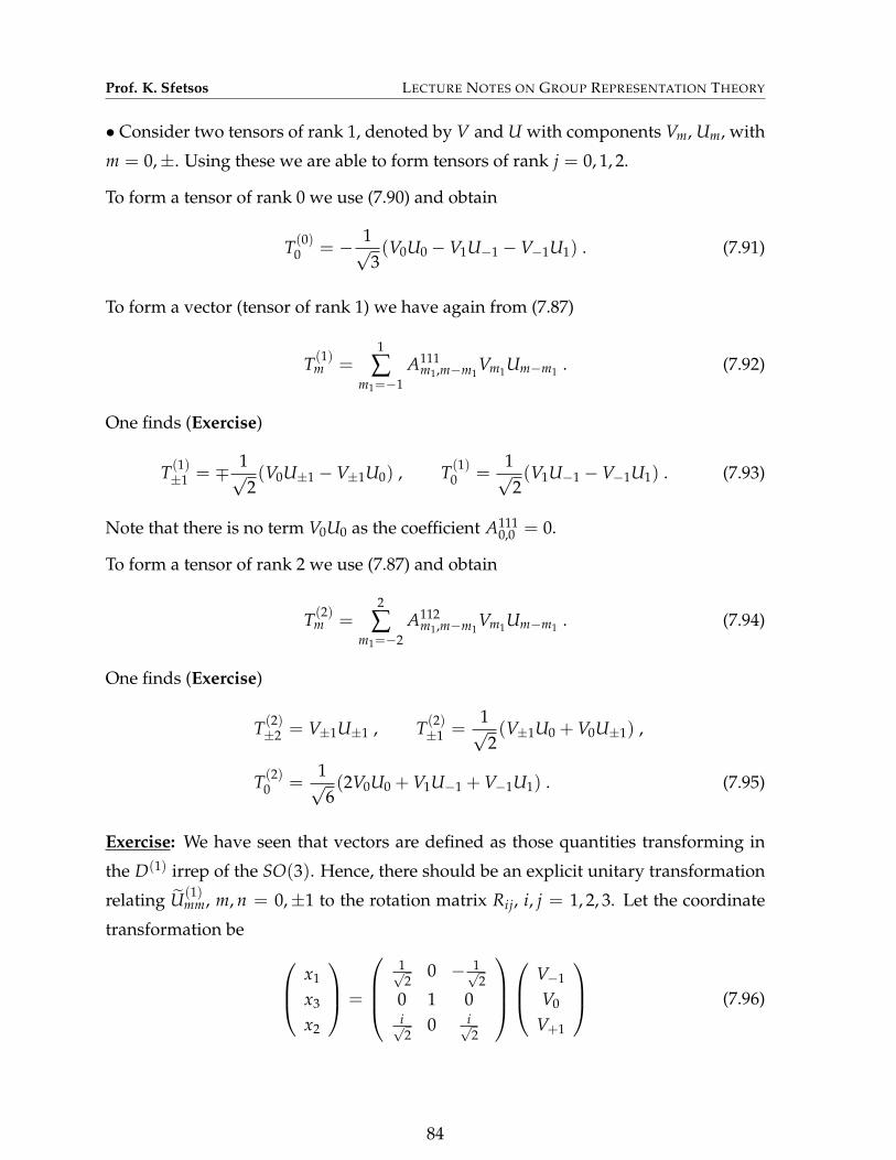
Prof. K. Sfetsos LECTURE NOTES ON GROUP REPRESENTATION THEORY
• Consider two tensors of rank 1, denoted by V and U with components Vm, Um, with
m = 0,±. Using these we are able to form tensors of rank j = 0, 1, 2.
To form a tensor of rank 0 we use (7.90) and obtain
T(0)0 = − 1√
3(V0U0 −V1U−1 −V−1U1) . (7.91)
To form a vector (tensor of rank 1) we have again from (7.87)
T(1)m =
1
∑m1=−1
A111m1,m−m1
Vm1Um−m1 . (7.92)
One finds (Exercise)
T(1)±1 = ∓ 1√
2(V0U±1 −V±1U0) , T(1)
0 =1√2(V1U−1 −V−1U1) . (7.93)
Note that there is no term V0U0 as the coefficient A1110,0 = 0.
To form a tensor of rank 2 we use (7.87) and obtain
T(2)m =
2
∑m1=−2
A112m1,m−m1
Vm1Um−m1 . (7.94)
One finds (Exercise)
T(2)±2 = V±1U±1 , T(2)
±1 =1√2(V±1U0 + V0U±1) ,
T(2)0 =
1√6(2V0U0 + V1U−1 + V−1U1) . (7.95)
Exercise: We have seen that vectors are defined as those quantities transforming in
the D(1) irrep of the SO(3). Hence, there should be an explicit unitary transformation
relating U(1)mm, m, n = 0,±1 to the rotation matrix Rij, i, j = 1, 2, 3. Let the coordinate
transformation be x1
x3
x2
=
1√2
0 − 1√2
0 1 0i√2
0 i√2
V−1
V0
V+1
(7.96)
84

Prof. K. Sfetsos LECTURE NOTES ON GROUP REPRESENTATION THEORY
and denote by Cim the components of the above 3× 3 unitary matrix. Show that
Rij =1
∑m,n=−1
CjmU(1)nmC−1
ni , (7.97)
or explicitly
R =
12(a2 + a∗2 − b2 − b∗2) i
2(a2 − a∗2 + b2 − b∗2) ab + a∗b∗
− i2(a2 − a∗2 − b2 + b∗2) 1
2(a2 + a∗2 + b2 + b∗2) i(a∗b∗ − ab)−(a∗b + ab∗) i(a∗b− ab∗) aa∗ − bb∗
(7.98)
and that this is precisely the matrix (7.8) (after flipping the signs of α0 and α1).
7.6 The Wigner–Eckart theorem
We are interested in deriving self-consistency relations between integrals of the form
T j1 jj2m1mm2 = 〈Ψj1m1 |T
(j)m |Φj2m2〉 , (7.99)
in a notation introduced in (5.11). With steps identical to those that led to (5.61) we
have that
T j1 jj2m1mm2 = ∑
m′1,m′,m′2
U(j1)∗(R)m′1m1U(j)(R)m′mU(j2)(R)m′2m2
T j1 jj2m′1m′m′2
, (7.100)
Next we use the Wigner coefficients and (7.61) to combine the last two U’s as
U(j2)(R)m′2m2U(j)(R)m′m =
j+j2
∑j=|j−j2|
Aj2 jjm′2m′A
j2 jjm2mU( j)(R)m′2+m′,m2+m . (7.101)
Then we obtain
T j1 jj2m1mm2 = ∑
m′1,m′,m′2, j
Aj2 jjm′2m′A
j2 jjm2mU(j1)∗(R)m′1m1
U( j)(R)m′2+m′,m2+mT j1 jj2m′1m′m′2
(7.102)
and we integrate next over dR. The l.h.s. is independent of R so that we simply pick
up a factor of hSU(2). For the r.h.s. we use the orthogonality theorem (7.56). We obtain
T j1 jj2m1mm2 = ∑
m′1,m′,m′2, j
Aj2 jjm′2m′A
j2 jjm2mδjj1
δm′1,m′2+m′δm1,m2+m
2j1 + 1T j1 jj2
m′1m′m′2. (7.103)
85

Prof. K. Sfetsos LECTURE NOTES ON GROUP REPRESENTATION THEORY
The δjj1 and the fact that |j− j2| 6 j 6 j + j2 implies that
|j− j2| 6 j1 6 j + j2 (7.104)
and that in the sum in (7.103) over j only one term survives. Then
T j1 jj2m1mm2 = Aj2 jj1
m2mδm1,m2+m ∑m′1,m′,m′2
δm′1,m′2+m′
2j1 + 1Aj2 jj
m′2m′Tj1 jj2m′1m′m′2
. (7.105)
The sum appearing in the r.h.s. depends only on j1, j2 and j. Hence, we have that
T j1 jj2m1mm2 = 〈Ψj1m1 |T
(j)m |Φj2m2〉 = Aj2 jj1
m2mδm1,m2+mΛj1 jj2 , |j− j2| 6 j1 6 j + j2 . (7.106)
This is the analog of (7.81) which was obtained for the scalar case. The quantity Λj1 jj2
denotes the triple sum in (7.105). It can be determined by computing just one of the
integrals on the l.h.s., for instance the one corresponding to m = 0 and then for m1 =
m2.
Exercise: Show that for a vector V
〈Ψj,m±1|V±|Φjm〉 = ∓
√(j∓m)(j±m + 1)
2j(j + 1)M(±)
j ,
〈Ψj,m|V0|Φjm〉 =m√
j(j + 1)Nj , (7.107)
for some M(±)j and Nj that do not depend on m.
7.6.1 Example of tensor decomposition
Any tensor of rank j can be decomposed into irreps of the rotation group. We will
explicitly work out all the details for how to assign these reps for rank 2 tensor Tij.
Such a tensor can be rewritten as
Tij = Ψ(0)δij + Ψ(1)ij + Ψ(2)
ij , i = 1, 2, 3 , (7.108)
where
Ψ(0) =T3
, Ψ(1)ij =
12(Tij − Tji) , Ψ(2)
ij =12(Tij + Tji)−
T3
δij (7.109)
86
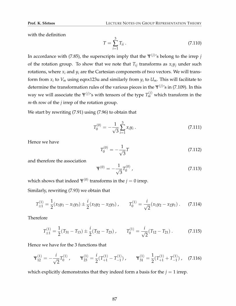
Prof. K. Sfetsos LECTURE NOTES ON GROUP REPRESENTATION THEORY
with the definition
T =3
∑i=1
Tii . (7.110)
In accordance with (7.85), the superscripts imply that the Ψ(j)’s belong to the irrep j
of the rotation group. To show that we note that Tij transforms as xiyj under such
rotations, where xi and yi are the Cartesian components of two vectors. We will trans-
form from xi to Vm using eqnx123u and similarly from yi to Um. This will facilitate to
determine the transformation rules of the various pieces in the Ψ(j)’s in (7.109). In this
way we will associate the Ψ(j)’s with tensors of the type T(j)m which transform in the
m-th row of the j irrep of the rotation group.
We start by rewriting (7.91) using (7.96) to obtain that
T(0)0 = − 1√
3
3
∑i=1
xiyi . (7.111)
Hence we have
T(0)0 = − 1√
3T (7.112)
and therefore the association
Ψ(0) = − 1√3
T(0)0 , (7.113)
which shows that indeed Ψ(0) transforms in the j = 0 irrep.
Similarly, rewriting (7.93) we obtain that
T(1)±1 =
12(x3y1 − x1y3)±
i2(x3y2 − x2y3) , T(1)
0 =i√2(x1y2 − x2y1) . (7.114)
Therefore
T(1)±1 =
12(T31 − T13)±
i2(T32 − T23) , T(1)
0 =i√2(T12 − T21) . (7.115)
Hence we have for the 3 functions that
Ψ(1)12 = − i√
2T(1)
0 , Ψ(1)23 =
i2(T(1)
+1 − T(1)−1 ) , Ψ(1)
31 =12(T(1)
+1 + T(1)−1 ) , (7.116)
which explicitly demonstrates that they indeed form a basis for the j = 1 irrep.
87

Prof. K. Sfetsos LECTURE NOTES ON GROUP REPRESENTATION THEORY
Using the above procedure we may also rewrite (7.95). We find that (Exercise)
T(2)±2 =
12(T11 − T22)±
i2(T12 + T21) ,
T(2)±1 = ∓1
2(T13 + T31)−
i2(T23 + T32) , (7.117)
T(2)0 =
1√6(2T33 − T11 − T22) .
There are 5 states in the j = 2 irrep (symmetric and traceless). A convenient basis is
Ψ(2)1 = Ψ(2)
23 , Ψ(2)2 = Ψ(2)
31 , Ψ(2)3 = Ψ(2)
12 ,
Ψ(2)4 =
1√2(Ψ(2)
11 −Ψ(2)22 ) , Ψ(2)
5 =1√6(2Ψ(2)
33 −Ψ(2)11 −Ψ(2)
22 ) . (7.118)
Using (7.117) we find that (Exercise)
Ψ(2)1 =
i2(T(2)
+1 + T(2)−1 ) , Ψ(2)
2 = −12(T(2)
+1 − T(2)−1 ) , Ψ(2)
3 = − i2(T(2)
+2 − T(2)+2 ) ,
Ψ(2)4 =
1√2(T(2)
+2 + T(2)−2 ) , Ψ(2)
5 = T(2)0 , (7.119)
indeed verifying that they form a basis for the j = 2 irrep.
Acknowledgments
I would like to thank Dr. A. Prinsloo and several students of the 2012-13 Academic
year for pointing out typos in the first version of these lecture notes.
Suggested bibliography
[1] W. Ledermann, Introduction to Group Characters, Cambridge University Press,
(1977).
[2] M. Tinkham, Group Theory and Quantum Mechanics, Dover, (2003).
[3] M. Hamermesh, Group Theory and its Applications to Physical Problems, Addison-
Wesley, (1989).
88