growing up in wartime: evidence from the era of two world wars · eief working paper 05/14...
TRANSCRIPT

IEF
EIEF Working Paper 05/14
September 2014
Growing up in wartime:
Evidence from the era of two world wars
by
Enkelejda Havari
(Università di Venezia “Ca’ Foscari”)
Franco Peracchi
(Università di Roma “Tor Vergata” and EIEF)
EIE
F
WO
RK
ING
P
AP
ER
s
ER
IEs
E i n a u d i I n s t i t u t e f o r E c o n o m i c s a n d F i n a n c e

Growing up in wartime: Evidence from
the era of two world wars∗
Enkelejda HavariUniversity of Venice “Ca’ Foscari”
Franco PeracchiUniversity of Rome “Tor Vergata” and EIEF
September 10, 2014
Abstract
We study the long-term consequences of war on health and human capital of Europeans bornduring the first half of the twentieth century, a period that has been termed the “era of twoworld wars”. This period includes not only WW1 and WW2, but also the Spanish Flu anda long series of armed conflicts which foreshadowed or followed the two world wars. Using avariety of data, at both the macro- and the micro-level, we address the following questions:What are the patterns of mortality and survival among people born during this era? What arethe consequences of early-life shocks on the health and human capital of the survivors some50 years later? Do these consequences differ by gender, socio-economic status in childhood, andage when the shocks occurred? We find that mortality is much higher in war- than in non-warcountries during WW1 and WW2, but not during the Spanish Flu. We also find importantdifferences between WW1 and WW2 in the mortality patterns by gender and age. As for thelong-term consequences of mortality shocks on the survivors, we find little evidence of increasedadult mortality for people born during WW1 and WW2, but some evidence for people bornduring the Spanish Flu, especially, in England and Wales, France and Italy. On the other hand,war-related hardship episodes in childhood or adolescence (in particular exposure to war eventsand hunger) are strong predictors of physical and mental health, education, cognitive abilityand wellbeing past age 50. The magnitude of the estimated effects differs by socio-economicstatus in childhood and gender, with exposure to war events having a larger impact on femalesand exposure to hunger having a larger impact on males. We also find that exposure to hungermatters more in childhood, while exposure to war events matters more in adolescence. Finally,we find that hardship episodes have stronger consequences if they last longer.
Key words: World War I; World War II; Spanish Flu; health; cognitive abilities; wellbeing;financial hardship; hunger; stress; socio-economic status; Europe; Human Mortality Database;
SHARE; ELSA.
JEL codes: I0, J13, J14, N34
∗ Corresponding author: Franco Peracchi ([email protected]). We thank Carlos Bozzoli, Janet Cur-rie, Angus Deaton, Marc Fleurbaey, John Londregan, Fabrizio Mazzonna, Andrea Pozzi, Jake Shapiro and JoachimWinter for helpful discussions. We also thank seminar participants at Princeton and the World Bank for usefulcomments. This paper uses data from SHARE release 2.5.0 as of May 24, 2011, SHARELIFE release 1 as of Novem-ber 24, 2010, and ELSA and ELSALIFE release 20 as of October 2013. The SHARE project has been primarilyfunded by the European Commission (see www.share-project.org for the full list of funders). The ELSA projecthas been funded by a consortium of U.K. Government departments and the U.S. National Institute on Aging (seehttp://www.elsa-project.ac.uk/funders for the full list of funders).

1 Introduction
Wars have been fought since ancient times and are still very frequent today. As Koestler (1978)
puts it, “the most persistent sound which reverberates through men’s history is the beating of war
drums.” Wars, or more generally armed conflicts at both the interstate and the internal level,
produce hardship, social disruption, and large losses of physical and human capital. According to
Amnesty International, “where wars erupt, suffering and hardship invariably follow. Conflict is
the breeding ground for mass violations of human rights including unlawful killings, torture, forced
displacement and starvation.”
The available macro-level literature suggests that the long-run effects of war on physical capital
are limited and can quickly be reversed. For example, Bellows and Miguel (2009) argue that “the
rapid postwar recovery experiences of some African countries after brutal civil wars – notably,
Mozambique and Uganda – suggest that wars need not always have persistent negative economic
consequences [. . . ] Other recent research has shown that the long-run effects of war on population
and economic growth are typically minor. Studies that focus on United States bombing [. . . ] find
few if any persistent impacts of the bombing on local population or economic performance. To the
extent that war impacts are limited to the destruction of capital, these findings are consistent with
the predictions of the neoclassical growth model, which predicts rapid catch-up growth postwar.”
As for human capital, although there is a sizeable literature on the effects of military service or
combat experience on earnings, health and mortality of veterans (see among others Angrist 1990,
1998, Angrist and Krueger 1994, Imbens and van der Klaauw 1995, Derluyn et al. 2004, Bedard and
Deschenes 2006, Betancourt et al. 2010, and Costa and Kahn 2010), much less is known about the
long-term consequences of armed conflicts and mass violence on the civilian population. Bozzoli et
al. (2008) argue that “the analysis of the consequences of mass violence for the economy during and
after its occurrence is a rather neglected field.” They also argue that “micro-level studies based on
surveys collecting qualitative and quantitative information on livelihood can provide insights into
channels of conflicts which cannot be analyzed on basis of macroeconomic indicators alone.”
It is useful to regard the long-term consequences of war on health, or human capital more
generally, as the net result of two distinct mechanisms: selection and scarring. Selection is the
effect on mean health due to changes in the composition of the population caused by differential
mortality. This effect is positive if the least healthy are more likely to die. Scarring is the long-
term damage to the individual health of survivors caused by war. In the model of Bozzoli, Deaton
and Quintana-Domeque (2009), the net effect of the two mechanisms is positive or negative and
1

varies substantially in magnitude depending on the level of mortality caused by an aggregate health
shock, which in turn is an increasing function of both the intensity of the shock and its degree of
persistence (that may itself depend on post-shock remediation). If scarring is not constant in the
population, the net effect may also depend on survivors’ heterogeneity.
In this paper we study the long-term consequences of war on health and human capital of
Europeans born during the first half of the twentieth century, a period that Berghahn (2006) calls
the “era of two world wars”. This period comprises not only World War I (1914–18) and World War
II (1939–45) but also a long series of armed conflicts, between and within European countries, such
as the Italo-Turkish war (1911–12), the Balkan wars (1912–13), the civil wars in Finland (1918) and
Germany (1918–19) and violence in Austria and Italy in the aftermath of World War I (WW1), the
Polish-Russian War (1919–21), the Greco-Turkish War (1919–22), the Austrian Civil War (1934),
the Spanish Civil War (1936–39), the Italian occupation of Albania (1939), the Greek Civil War
(1946–49), and violence in Central and Eastern Europe in the aftermath of World War II (WW2).
We address three main questions: What are the patterns of mortality and survival among people
born during the era of two war wars? What are the consequences of early-life shocks on the health
and human capital of the survivors some 50 years later? Do these consequences differ by gender,
socio-economic status in childhood, or age when the shock occurred? Unlike other papers, we do
not try to identify causal effects or some policy-relevant parameter, as we do not see in our data
credible sources of exogenous variation that we can exploit. We also make no attempt at modeling
the very complicated process that links the individual experience of war-related shocks in childhood
or adolescence to adult outcomes. Still, two considerations make our analysis potentially relevant
for policy. First, the cohorts that experienced WW2 in their childhood or adolescence represent the
bulk of the population aged 70 and older in Europe. The link to specific war-related experiences
may help understand their health patterns. Second, our findings may be useful for understanding
the long-term consequences of recent armed conflict, for which no long-term data is yet available.
WW1 and WW2 were the deadliest wars in human history in absolute terms, though not
in relative terms (see e.g. Diamond 2012), but estimates of war-related casualties are subject to
considerable uncertainty. The estimated death toll of WW1 in Europe ranges between 12 and
14 millions (2.5–3 percent of the total population in 1914). The estimated death toll of WW2
in Europe is three to four times higher, ranging between 40 and 50 millions (7–9 percent of the
total population in 1940), the large uncertainty reflecting the death counts for Germany, Greece,
Poland, the Soviet Union and Yugoslavia. There are no reliable estimates of the death toll of the
2

other armed conflicts in Europe during this period, but estimates for the Spanish Civil War range
between 190,000 and 500,000 deaths. As argued by Berghahn (2006, p. 7), “Europe had not seen
mass death on such a scale since the Thirty Years War of the seventeenth century.”
Between WW1 and WW2, two health catastrophes – the Spanish Flu (1918–21) and the
Ukrainian Famine (1932–33) – added at least another 6 millions to the death count. The Spanish
Flu claimed about 3 million lives in Europe (Ansart et al. 2009), making it one of the deadliest
natural disasters in history. Excess death from the Spanish Flu in Europe is estimated at 1.0–
1.2 percent of the total 1918 population. Erkoreka (2009) suggests a direct link between WW1
and the Spanish Flu, as “the millions of young men who occupied the military camps and trenches
were the substrate on which the influenza virus developed and expanded.” The Ukrainian Famine
claimed more than three million lives. Snyder (2010, p. 53) estimates that “no fewer then 3.3
million Soviet citizens died in Soviet Ukraine of starvation and hunger-related diseases.”
The larger death toll of WW2 relative to WW1 reflects not only the enhanced destructive
power of weapons, but also the longer duration of the war, its wider geographical spread, and
the greater level of involvement of the civilian population. A very crude measure of the latter is
the ratio of civilian to total deaths. Estimated civilian deaths in Europe are about 5 millions for
WW1 and 20–28 millions for WW2 (three fourths of them in the “bloodlands” of Belarus, Poland,
Ukraine, the Baltic States and some of Russia’s western fringe). These numbers represent about
40 percent of total human losses in Europe during WW1 and about 60 percent during WW2, with
a huge cross-country variability. Key factors that help explain the higher burden of WW2 on the
civilian population are the direct impact of war operations and “strategic bombing” on civilians,
war-related hunger and disease, and deliberate mass murder of targeted population groups (most
notably, Jews).
Apart from the aggregate death toll, we have very little statistical evidence on the consequences
of WW1 for the civilian population. For example, Berghahn (2006, p. 45) observes that “to this day
we have no reliable statistics on diseases among the civilian population and its fate more generally.
What we can say is that for many regions it was no less than disastrous.” Recently, Borsch-Supan
and Jurges (2012) provide some illustrative evidence showing a substantial hike in early retirement
rates (before age 55) among German men and women born during the hunger years of WW1 (1917–
18). For the Spanish Flu, we have the evidence in Almond (2006) and Brown and Thomas (2013)
for the USA, and several epidemiological studies for Europe.
Unlike the survivors of WW1 and the Spanish Flu, who are now mostly dead, a relatively large
3

fraction of people who survived WW2 are still alive today and able to recall their experience of
specific shocks and hardship episodes. The recent availability of data covering survivors of WW2
has stimulated a growing literature that focuses on the channels through which war affects the
civilian population, especially children and adolescents.
The main channels considered sofar are the disruption of the educational process through phys-
ical destruction, loss of educators, school closure or conscription of students (Ichino and Winter-
Ebmer 2004, Akbulut-Yuksel 2014), the loss of parents during war, the increased risk of prosecution
and dispossession, and exposure to hunger or even famine (Havari and Peracchi 2011, van den Berg,
Pinger and Schoch 2012, Jurges 2013, and Kesternich et al. 2014). All available studies find impor-
tant negative consequences of experiencing war-related hardship on education, health and earnings
of survivors. These negative consequences may be linked, as lower educational attainments imply
large earnings losses but may also impact other domains, such as physical and mental health.
Relative to the economic literature focusing on WW2, our work is novel in several respects. First,
we take a longer historical perspective, from the beginning to the middle of the twentieth century.
Second, we consider a larger set of countries, including England, Spain, and the Scandinavian
countries. Extending the analysis to England is particularly important because of the crucial role
of this country in both world wars and because its food and health policies were very different
from those in continental Europe (for WW2, see Collingham 2011). Third, we exploit the macro-
level information contained in country-specific mortality data by age, gender and year. Fourth,
at the micro-level, we study the relationship between experiencing various types of hardship in
childhood or adolescence and a broad set of adult outcomes, including physical and mental health,
cognitive ability and wellbeing. We also consider differences between people who experienced
hardship episodes at different ages in childhood or adolescence.
Our work is also related to three recent strands of the literature. The first is the child de-
velopment literature, which emphasizes the importance of early life conditions for adult outcomes
(Almond 2006, Currie and Moretti 2008, Almond and Currie 2011a) and the role of particular
critical periods for certain outcomes (Case, Fertig and Paxson 2005, Cunha and Heckman 2007,
Case and Paxson 2008, 2010, Currie 2009, 2011).
The second is the literature that uses extreme and sharp events, such as famines, in order to
identify causal relationships of interest. Interestingly, three widely studied famines are directly
related to WW2: the Greek famine of 1941–42 (Neelsen and Stratmann 2011), the Leningrad
famine of 1941–44 (Sparen et al. 2004), and the Dutch Hunger Winter of 1944–45 (Ravelli, van
4

der Meulen and Barker 1998, Roseboom, de Rooij and Painter 2006, Lumey, Stein and Susser
2010). Most of this literature focuses on the long-run effects of nutritional deficiencies around
birth, or Barker’s “fetal origins hypothesis” (see e.g. Almond and Currie 2011b, and Dercon and
Porter 2014). Its main finding is that exposure to hunger or famine around birth or early childhood
negatively influences a variety of health and non-health outcomes at much later ages.
The third is the recent literature on the short-term effects of civil wars and armed conflicts in
Africa and Asia (Alderman, Hoddinott and Kinsey 2006, Bellows and Miguel 2009, Bundervoet,
Verwimp and Akresh 2009, Blattman and Annan 2010, Shemyakina 2011, Akresh et al. 2012,
Minoiu and Shemyakina 2012, Ampaabeng and Tan 2013). Its main finding is that exposure to
armed conflicts has severe negative effects on the health of exposed children.
The remainder of this paper is organized as follows. Section 2 presents our data. Section 3
focuses on country-level data and describes the patterns of mortality for the cohorts born during
the first half of the twentieth century. Section 4 focuses on micro-level data and studies the
relationship between war and the experience of hardship episodes for individuals born between
1930 and 1956 who were alive 50 years later or more. Section 5 uses these micro-level data to
analyze the consequences on later life outcomes of exposure to war and hardship during childhood
or adolescence. Finally, Section 6 summarizes and concludes.
2 Data
We combine three types of data. The first type is death rates by country, age, year and gender from
the Human Mortality Database (HMD), a joint project by the Department of Demography at the
University of California Berkeley and the Max Planck Institute for Demographic Research, which
provides detailed and comparable data for eleven European countries over a long time period.
The second is rich micro-level data from two multidisciplinary household panel surveys, namely
the Survey of Health, Ageing and Retirement in Europe (SHARE) and the English Longitudinal
Study of Ageing (ELSA). Both surveys collect extensive information on socio-economic status
(SES), health, social and family networks from nationally representative samples of people aged
50+ in participating countries, including detailed life-history data.
The third, relevant for the cohorts covered by SHARE and ELSA, is detailed and accurate
information on war events during the Spanish Civil War and WW2.
5

2.1 HMD
Death rates in the HMD are obtained as the ratio between death counts and counts of the population
at risk, the raw data generally consisting of birth and death counts from vital statistics, plus
population counts from periodic censuses or official population estimates (see Wilmoth et al. 2007
for details).
The HMD contains mortality data starting from 1890 or earlier for eleven Western European
countries, namely Belgium, Denmark, England and Wales, Finland, France, Italy, the Netherlands,
Norway, Spain, Sweden and Switzerland. Unfortunately, data for Belgium are missing for the WW1
period (1914–18). Due to changes in borders and mass population movements, mortality data for
Austria, Germany and all Eastern European countries are only available after WW2, often only
after 1955. As a result, the HMD only offers a partial view of the patterns of mortality during the era
of two world wars. This is a major limitation because both world wars were much more devastating
in Eastern Europe (Berghahn 2006). With reference to WW2, Davies (2006, p. 24) argues that
“the war assumed a far grander scale in the East than in any of the fronts where the Western Allies
were involved.” Again with reference to WW2, Snyder (2010, p. 394) points out that “German and
Soviet occupation together was worse than German occupation alone. The populations east of the
Molotov-Ribbentrop line, subject to one German and two Soviet occupations, suffered more than
any other region of Europe.”
2.2 SHARE and ELSA
For thirteen continental European countries, namely Austria, Belgium, Czech Republic, Denmark,
France, Germany, Greece, Italy, the Netherlands, Poland, Spain, Sweden and Switzerland, we
combine the information from the second and the third wave of SHARE. Notice that the survey
does not include England and Wales, Finland and Norway, which are covered by the HMD, but
includes countries for which we lack long-term mortality data, most notably Germany and Poland.
Its second wave (2006–07) collects information on the current status of survey participants, in
particular their health and SES. Its third wave (2008–09), also known as SHARELIFE, collects
retrospective information on employment, health and accommodation histories, experience and
duration of hardship episodes, and childhood circumstances around age 10. For England, we
combine the information on current status from the second wave (2004–05) of ELSA with the
retrospective information from ELSALIFE, the life-history interviews in its third wave (2007).
SHARE and ELSA were designed to help understand the patterns of aging in Europe. Both
6

surveys interview nationally representative samples of people aged 50+ at the time of the inter-
view, who speak the official language of the country and do not live abroad or in an institution.
Spouses or partners are included irrespective of age. A key aspect of both surveys, which makes
them particularly suited for our purposes, is the detailed retrospective information they collect
on individual life histories. We exploit this information to construct a longitudinal data set with
annual observations on the occurrence of a number of events.
Although SHARE and ELSA are similar in scope, coverage and organization, several important
differences prevent us from merging the two datasets and force us to analyze them separately.
In this section we summarize the main differences and refer to Appendix A for a more detailed
description.
A unique feature of the public use version of SHARELIFE is the information it provides on the
residence in which the respondents lived when they were born and on each subsequent residence in
which they lived for six months or more, including the start and end year, the type of residence,
and the country, region and area where the residence was located. A drawback is the fact that
the level of regional disaggregation varies by country: it is at the coarse NUTS1 level for Belgium,
Denmark, France and the Netherlands, at the fine NUTS3 level for the Czech Republic, and at the
intermediate but not very detailed NUTS2 level for all other countries. Unfortunately, the public
use version of ELSALIFE provide little information on past residence and no information that can
be used to determine the country and region of residence in a given year. Basically, we can only
determine whether the respondent was living in the U.K. or abroad in a given year.
As for SES in childhood, both surveys collect broadly comparable information on the occupation
of the main breadwinner (SHARELIFE) or the respondent’s father (ELSALIFE), the number of
books at home, the main features of the accommodation, and the household size and composition
when the respondent was aged 10. We use this information to construct an index of SES in childhood
based on principal component analysis (PCA) and indicators for the absence of the parents when
the respondent was aged 10.
As for childhood health, SHARELIFE collects information on self-reported health (SRH), the
distinct illnesses experienced by the respondents in childhood, and the age interval (0–5, 6–10 and
11–15) in which each illness was experienced. ELSALIFE also collects information on SRH and the
distinct illnesses experienced by the respondents in childhood, but no detail on their timing.
As for hardship episodes in childhood, SHARELIFE asks whether there was a distinct period
during which the respondents experienced stress, poor health, financial hardship or hunger, and
7

the year when this period started and ended. Although we have no information on the intensity of
a hardship, we can determine its duration by taking the difference between the year it ended and
the year it started. Notice that respondents are asked to report only one episode for each type of
hardship, presumably the most salient (phrases such as “distinct period” or “compared to the rest
of your life” are meant to capture this idea). Further, hardships are not defined precisely and their
perception may vary across individuals, which raises the issue of interpersonal comparability. This
may be especially problematic for hunger, as we do not know exactly how respondents interpret the
question. Financial hardship is the only type of hardship considered by ELSALIFE. We only know
the age when financial hardship started but not when it ended, so duration cannot be computed.
On the other hand, ELSALIFE differs from SHARELIFE because it collects direct information on
war exposure by asking whether respondents witnessed serious injury or death of someone in war
or military action and whether they were evacuated during WW2.
The adult outcomes that we consider include SRH as an overall measure of health, indicators
of physical and mental health, educational attainments, and measures of numeracy and recall
ability. We also consider two dimensions of subjective wellbeing, namely life satisfaction and
happiness. As discussed by Kahneman and Deaton (2010), life satisfaction refers to the thoughts
people have about their life, while happiness (or, perhaps more precisely, emotional wellbeing)
reflects the emotional quality of individual’s everyday life. This distinction is important because
the two dimensions correlate differently with income and health outcomes. While the information
on SRH, recall ability, life satisfaction and happiness is fairly comparable in SHARE and ELSA,
important differences arise with the other outcomes. First, the numeracy test is not administered
in waves 2 and 3 of ELSA, and the only available measure of cognitive ability is an indicator of
memory (recall total). Second, unlike SHARE, ELSA does not collect detailed information on the
chronic conditions diagnosed. Third, unlike SHARE, body height and weight in ELSA are not
self-reported but are objective measures taken during a nurse visit which is a key component of the
survey. Fourth, SHARE collects information on the years of completed schooling, while ELSA asks
the age at which the respondent left full time education. Fifth, SHARE uses the Euro-D index of
depression, which considers several dimensions of mental health (depression, anxiety, suicidality,
etc.), while ELSA only asks whether the respondent was feeling depressed in the past week.
Like most household surveys, both SHARE and ELSA suffer of sample attrition and item
nonresponse. In addition, specific problems with the life-history data collected in the two surveys
include recall bias, coloring and limited information on certain variables.
8

Despite the adoption of preventive procedures, such as training of the interviewers and survey
design characteristics, sample attrition is an important feature of both surveys. The level of attrition
varies by country and is determined by many factors, such as age, gender and education.
Item nonresponse arises when individuals do not answer a particular question. In household
surveys, this is a major problem for income and assets, but is usually a minor problem for health
and wellbeing. SHARE and ELSA are no exceptions (Borsch-Supan and Jurges 2005). In both
surveys, nonresponse is important for income and wealth, but is unimportant for health, hardships
and childhood circumstances.
Recall error arises when respondents do not remember precisely when and how an event took
place in the past. There are concerns that retrospective data suffer from recall errors especially
when the population of interest consists of elderly people. In fact, Havari and Mazzonna (2014) find
little evidence of both. This partly reflects a distinctive advantage of SHARELIFE and ELSALIFE
over other surveys, namely the fact that both apply the life-history calendar method, which is based
on temporal landmarks (events that are striking or easier to remember) and should therefore lead
to better accuracy (see for example Groves et al. 2004).
Even when an event is a temporal landmark, one cannot rule out coloring, namely the fact that
respondents may answer questions about the distant past based on post-event information, such as
their current status or macro-events that are part of a country’s narrative. We find little evidence
of coloring in SHARE and ELSA when using information on hardships.
2.3 Major war events
Although SHARE does not collects direct information on war exposure, knowledge of the country
and region of residence of the respondents in each single year allows us to construct an indicator
of potential war exposure by exploiting historical information on major war events (both combat
operations and aerial bombings) during the period between the beginning of the Spanish Civil
War in 1936 and the end of WW2 in 1945. Things are just the opposite for ELSA, which collects
direct information on war exposure but lacks the temporal and spatial information needed to relate
individual experiences to major war events.
For the Spanish Civil War, our main sources of information are Thomas (2003) and Preston
(2006), while for WW2 we exploit a variety of sources, including Ellis (1994) and Davies (2006). We
refer to the regions affected by major war events as “war regions”. The remainder of this section
provides some detail for the SHARE regions.
9

The Spanish Civil War began in July 1936 and initially affected all regions of Spain, except
Ceuta and Melilla and the Canary Islands. In 1937 it mostly affected the central, south-eastern,
eastern and northern regions. In 1938 and 1939 it mostly affected its central, south-eastern and
eastern regions. The Spanish Civil War conventionally ended on April 1, 1939. Exactly five months
later, on September 1, 1939, WW2 began with the German invasion of Poland, coordinated with
the Soviet invasion from the east on September 17. Thus, for 1939, our war regions include the
whole of Poland and some regions of Spain. The regions along the French-German border are
not included because only affected by small-scale war operations (the so-called ”phony war”). In
1940, our war regions include the whole of Belgium and the Netherland, and the northern and
eastern regions of France. In 1941, they include the whole of Greece, plus the German regions of
Bremen and Hamburg that were subject to heavy aerial bombing. In 1942, no region considered
in SHARE was affected by major combat operations, and our only war regions are some heavily
bombed regions of Germany. In 1943, combat was limited to the southern Italian regions, but
aerial bombing of Germany extended and intensified. In 1944, combat affected eastern Poland,
central Italy, most of Greece, and parts of Belgium, France and the Netherlands, while large parts
of Germany were under heavy aerial bombing. In 1945, our war regions include all of Germany,
central and western Poland, northern Italy, eastern Austria, most of the Czech Republic, and parts
of Belgium, France and the Netherlands. In Europe, WW2 conventionally ended on May 8, 1945
with the unconditional surrender of all German forces to the Allies.
Notice that, although mainland Denmark was under German occupation from April 1940 to the
end of WW2, we do not include its regions among the war regions because they were never affected
by major war events. More generally, “even countries which suffered grievously from fighting and
occupation could have large expanses of their territory virtually untouched” (Davies 2006, p. 17).
3 Mortality and survival
In this section we use the HMD data to illustrate the patterns of mortality for the cohorts born
during the first half of the twentieth century in the countries for which we have long-run mortality
data. These cohorts have experienced severe mortality shocks earlier in life, so it is important
to describe the main features of the selection process caused by mortality during this period.
Furthermore, since our micro-level data comes from people who were alive at the time of the
SHARE or ELSA interviews, we also provide some evidence on survival rates by country, gender
and cohort.
10

3.1 Mortality patterns
Figures 1 and 2 present contours plots of death rates by age during the period 1890–2009, sep-
arately by country and gender (green ≤ .1 percent, light blue .2–.8 percent, blue .8–3.0 percent,
purple 3–7 percent, red > 7 percent). For simplicity, we only show the results for three countries
that participated to both WW1 and WW2, namely England and Wales, France and Italy. As a
comparison, we also include one country that was neutral during both world wars, namely Sweden.
We consider all years of age from 0 to 80 and all calendar years from 1890 to 2009.
The figures reveal a clear downward trend in mortality, interrupted by sharp increases during
the years of WW1, the Spanish Flu and WW2. They also show that the mortality patterns
during these three episodes differ substantially by country, gender and age group. First, death
rates were much higher in war countries during WW1 and WW2, but not during the Spanish Flu.
Second, they were much higher for males than for females during WW1 and WW2, but again
not during the Spanish Flu. Third, they were higher for younger adults, especially young males
subject to military service. Fourth, for France we observe a bimodal profile of mortality during
WW2, with one peak in 1940 and another one in 1944–45, corresponding to the start and the
end of German occupation. A similar pattern can be observed for Belgium, the Netherlands and
Norway, also occupied by Germany during WW2. As argued by Berghahn (2006, p. 101), “in the
west and north a measure of normalcy did return after the respective armies had been defeated by
the Wehrmacht’s powerful strokes. Only after 1942–43 did these countries experience a renewed
escalation of violence.” Finally, for all three war countries there is some evidence of higher mortality
at older ages for the cohorts aged 20–30 during WW1 and for the cohorts born around the time of
the Spanish Flu. However, the latter cohorts were unlucky enough to be aged 20–30 during WW2,
so it is hard to distinguish the scarring effects of the Spanish Flu from those of WW2.
To complement the visual information from Figures 1 and 2, and to isolate the long-term
consequences of living though our three high-mortality episodes, we consider the following flexible
model for the age profile of cohort-specific log death rates, lnmx, by country and gender
E(lnmxab) = f(a) + g(b) + h(a, b) +∑i
αiAi +∑j
βjTj +∑i
∑j
γijAi ∗ Tj +∑k
δkBk, (1)
where f(a) is a cubic spline in age a (expressed in deviation from age 50), g(b) is a cubic polynomial
in the year of birth b (expressed in deviation from year 1935), h(a, b) is a quadratic interaction term
between age and birth year introduced to capture changes in the age-profile of mortality across
cohorts, the Ai are a set of age dummies for being aged 18–27 and 28–37 introduced to capture
11

the existence of a “mortality hump” for younger adults reflecting accident mortality for males and
accident plus maternal mortality for females (Heligman and Pollard 1980), the Tj are a set of
time dummies for the years of WW1 (1914–18), the Spanish Flu (1919–21) and WW2 (1939–45),
and the Bk are a set of cohort dummies for being born during WW1, the Spanish Flu or WW2.
The term f(a) + g(b) + h(a, b) is a smooth function of age and birth year that captures long-run
trends in mortality at ages different from 18–37, the αi coefficients measure the excess mortality
for younger adults (age groups 18–27 and 28–37) in “normal” years, the βj coefficients measure
the excess mortality during WW1, the Spanish Flu and WW2 at ages different from 18–37, the
γij coefficients measure the excess mortality during WW1, the Spanish Flu and WW2 for younger
adults, and the δk coefficients measure the long-run consequences of being born during WW1, the
Spanish Flu or WW2. All coefficients have the interpretation of percentage differences relative to
the long-run trends. The model is estimated separately by country and gender via ordinary least
squares (OLS) using all ages from 0 to 99 and all calendar years from 1890 to 2009.
Table 1 presents the estimates of the coefficients in model (1), separately by country and gender,
along with the sample size (N) and the adjusted R2 (R2a), separately by country and gender, with
the top panel for females and the bottom panel for males. The stars denote p-values, with * for
p-values between 5 and 10 percent, ** for p-values between 1 and 5 percent, and *** for p-value
below 1 percent.
For the age groups 18–27 and 28–37, excess mortality is always positive, large and statistically
significant in all countries, confirming the existence of a mortality hump for younger adults. For
the age group 18–27 this effect is much stronger for males than for females, while for the age group
28–37 it is about the same for both genders. In all countries, baseline excess mortality during WW1,
the Spanish Flu and WW2 is always higher for males than for females, gender differences being
especially large during WW1. Further, during all three periods, the mortality hump for younger
adults is magnified, especially in war countries (England and Wales, France and Italy during both
world wars, and Finland during WW2). Not surprisingly, excess mortality in war countries is much
higher for younger males than for younger females. For males aged 18–27, excess mortality during
WW1 is also higher in England and Wales and France than in Italy, partly because Italy joined the
war about one year later. During WW2, it is particularly high in Finland, where it is nearly twice
that observed in England and Wales, France and Italy, to testify the intensity of the Russian-Finnish
wars of 1939–40 and 1941–44. In non-war countries, instead, gender differences in the mortality
hump for younger adults are much smaller or are even reversed. There is some evidence of a scarring
12

effect on mortality at later ages for females and males born during WW1 in war countries, but the
scarring effect for people born during the Spanish Flu appears to be very weak. Being born during
WW2 is instead associated with a permanent decrease in mortality for both females and males in
all countries, including those directly exposed to the war. This may reflect selection effects, but
also the rapid economic recovery and the policies adopted in the postwar period.
To summarize, WW1, the Spanish Flu and WW2 are all characterized by strong upward devi-
ations from the long-run trend of falling mortality, but the magnitude of the three shocks varies
considerably by country, gender and age group. As for the long-run consequences of these mortality
shocks, WW1 and the Spanish Flu leave recognizable scars on survivors, most notably in our three
war countries – England and Wales, France and Italy. This does not appear to be true for WW2,
as people born during the war are characterized by lower mortality at later ages. Possible reasons
for this difference include postwar remediation, rapid increase in postwar income, improvements in
health care, etc.
3.2 Survival rates up to the SHARE and ELSA interviews
Since SHARE and ELSA only interview people who reached age 50 at the time of the interview, it is
important to understand how selected the reference population is. We use the HMD to address this
issue for the nine countries for which we have both micro-level and mortality data, namely Belgium,
Denmark, France, England (and Wales), Italy, the Netherlands, Spain, Sweden and Switzerland.
Tables B1 and B2 in Appendix B show the survival rates up to year 2006 for the cohorts born
between 1918 and 1956, separately by country and gender. Survival rates have been constructed
by multiplying annual survival probabilities (i.e., one minus the death rates) from the year of birth
(when they are set equal to 1) to 2006, separately by gender, country and cohort.
Survival rates increase with the year of birth and are always higher for women. For example,
about two thirds of the women born in 1930 were still alive in 2006, but only about half of the men
born in 1930 were still alive. As another way of saying this, survival rates of men born in 1930 are
similar to those of women born six years earlier, in 1924. Survival rates also vary a lot by country.
For example, for females born in 1930, they are highest in Switzerland (.745), France (.721) and
Sweden (.717), and lowest in England and Wales (.641) and Denmark (.603). For men born in the
same year, they are highest in Switzerland (.556) and Sweden (.554), and lowest in Spain (.477)
and Denmark (.472). These cross-country differences depend in a complicated way on a number
of factors that include more than just war-induced mortality and the experience of hardship in
13

childhood and adolescence.
An open issue, discussed in Section 5.2.4 is how this selection process affects the estimated
relationship between hardship in childhood and adult outcomes.
4 War and hardship in childhood
We now consider the relationship between war and the experience of hardship episodes – stress,
absence of the parents at age 10, financial hardship and hunger – among SHARE and ELSA
respondents born between 1930 and 1956.
In Sections 4.1–4.4 we exploit the longitudinal dimension of SHARELIFE (see Section 2) and
study the prevalence of the various types of hardship among our cohorts of SHARELIFE respon-
dents. We do not consider poor health because most of the reported episodes occur later in life.
In Section 4.5 we present comparable evidence from ELSALIFE. Our main conclusion is that the
Spanish Civil War, WW2 and their immediate aftermaths are closely associated with many of the
hardship episodes experienced by people in our sample, in particular stress, absence of the father
and hunger.
4.1 Stress
Figure 3 shows the prevalence of stress during the period 1935–65 for people born between 1930
and 1956. Here and in what follows we use red vertical bars to mark the WW2 period (1939–45).
There is some evidence of an association between stress and war, as the prevalence of stress reaches
relatively high levels during the WW2 period in France and Poland, and peaks in 1945 in Austria,
Belgium, France, Germany and Italy. However, the prevalence of stress tends to increase during the
postwar period in many countries, suggesting that stress is also strongly associated with adulthood.
Figure 4 focuses on those who report experiencing a period of stress before age 17 and shows
the cumulative distribution function of its starting and ending year for all countries except Den-
mark (only subject to a mild German occupation) and the two neutral countries (Sweden and
Switzerland). The figure confirms an association, albeit weak, between stress and war.
Miller and Rasmussen (2010) emphasize the importance of daily stressors, that is a series of
conditions and circumstances of everyday life that can worsen the psychological state of an indi-
vidual who has been directly exposed to a conflict. Among the daily stressors that can amplify the
negative effect of war exposure are the absence of the parents, financial hardship and hunger, for
which SHARELIFE also provides evidence.
14

4.2 Absence of the parents
Figure 5 shows the fraction of SHARE respondents born between 1930 and 1956 who report absence
of the parents at the age of 10 in each calendar year between 1935 and 1965. It differs from the
other figures because we lack information on the year when absence of the parents began or ended.
In all countries, fathers are more likely to be absent than mothers. Further, unlike absence of
mothers, absence of fathers displays a clear temporal pattern, at least in Austria, France, Germany,
Poland and, to a lesser extent, Italy and Spain. In Austria and Germany the percentage of respon-
dents reporting an absent father is particularly high towards the end of WW2 and in its immediate
aftermath, when it reaches a peak of over 30 percent. The pattern observed for France and Poland
is similar but less pronounced.
This evidence is broadly consistent with the fact that POWs, mostly males, were used as forced
labor by both Germany and the Soviet Union during WW2, and by the Soviet Union even after
the war. Repatriation took a long time, the last German prisoners of war returning home only in
1956 (Davies 2006), while about 600,000 Germans taken as POWs or laborers would die (Snyder
(2010, p. 318).
4.3 Financial hardship
Figure 6 shows the prevalence of financial hardship during the period 1935–65 among people born
between 1930 and 1956. Although the link between war and financial hardship is not very strong,
there is a clear evidence of concentration of financial hardship episodes during the WW2 period
in Italy, Greece and Poland, and in the aftermath of WW2 in Germany and of the Civil War in
Spain. Two countries stand out as somewhat exceptional. One is Germany, where the prevalence
of financial hardship is quite low until the very end of WW2. The other is Greece, for both the
high prevalence of financial hardship in the prewar period (more than 5 percent) and the fact that
prevalence jumps to about 10 percent at the beginning of the Balkans campaign of WW2 in 1940
and then declines steadily afterwards.
Figure 7 focuses on those who report experiencing a period of financial hardship before age
17 and shows the cumulative distribution function of its starting and ending year for all countries
except Denmark, Sweden and Switzerland. The figure confirms an association between financial
hardship and war or its immediate aftermath.
15

4.4 Hunger
Figure 8 shows the prevalence of hunger during the period 1935–65 among people born between 1930
and 1956. The figure reveals a strong link between hunger and either war or the immediate postwar
period. In Belgium, France, Greece, Italy, the Netherlands and Poland, the prevalence of hunger
is very high during the WW2 period. In France, Greece, Italy and Poland about 10 percent of our
respondents report experiencing hunger during the WW2 years. In the Netherlands, we observe a
sharp increase of hunger episodes in 1944 and 1945, corresponding to the “Hunger Winter” in the
German occupied part of the country, but very little evidence of hunger in the post-WW2 period.
In Austria and Germany, instead, hunger episodes are concentrated in 1944–45 and the immediate
aftermath of WW2. Germany is the country where the prevalence of hunger is highest, with nearly
one fourth of our German respondents reporting this hardship in 1945. In Spain, a large fraction of
reported hunger episodes begins not during the Civil War but rather in its aftermath, with a peak
in 1940. On the other hand, there is little evidence of hunger for the neutral countries, Switzerland
and Sweden. This is also true for the Czech Republic and Denmark, despite the German occupation.
Collingham (2011, p. 218) argues that “it was not until after the war that the German civilian
population began to suffer from inadequate rations [. . . ] While Germans were well supplied between
1939 and 1945 their European neighbours were systematically plundered, murdered and deliberately
starved to death for the sake of a secure food supply for German civilians.” In particular, as pointed
out by Jan Karski in his 1944 report, “poverty and the malnutrition [...] had increased in Poland by
the deliberate design of the Germans to a point where the health of the entire nation was seriously
threatened” (Karski 2013, p. 235). These observations are consistent with the evidence in Figure 9,
which shows the cumulative distribution function of the year when the hunger episode is reported
to start and to end for those who report experiencing hunger before age 17. We exclude Denmark,
Sweden and Switzerland because the prevalence of hunger is very low. In Austria and Germany,
most reported hunger episodes start at the end of the war in 1945 and their end is spread over the
next 3 to 4 years. In the Netherlands, instead, they mostly start in 1944 and mostly end in 1945.
In Belgium, France, Greece and Italy, a substantial fraction of hunger episodes starts in 1940 and
ends in 1945. In Poland, they mostly begin in 1939 or 1940 and end in 1945. In Spain, instead, a
substantial fraction of reported hunger episodes begins in 1936 or 1940 and ends in 1945 or 1951.
To illustrate the close association between hunger and war events, Figure 10 shows their regional
distribution in Europe. The two top panels show the percentage of respondents having ever suffered
hunger between 5 and 16 years of age, separately for the cohorts born in 1930–39 (top-left panel)
16

and 1940–49 (top-right panel). The regional disaggregation reflects the actual level of geographical
detail available in SHARELIFE. Comparing the two panels reveals that the cohorts more exposed
to hunger are those born in 1930–39, mainly because of their exposure to war. In the top-left panel,
the color gets darker in many regions of Poland, Germany, France, Spain, Southern Italy, Eastern
Greece, etc., with 20–50 percent of respondents suffering hunger, whereas in the top-right panel
everything is lighter.
The bottom panel shows the number of years of potential exposure to war for exactly the same
regions during the period from the beginning of the Spanish Civil War in 1936 to the end of WW2 in
1945. The shading in the map becomes darker as the number of years of potential exposure to war
increases. The darkest color, corresponding to three years or more, is for some regions of Belgium,
Eastern France and the Netherlands (ravaged by war first in 1940 and a second time in 1944–45),
the Berlin, Bremen, Hamburg and Ruhr regions in Germany (subject to heavy aerial bombing
from 1942 to 1945 and to combat in 1945), the regions around Warsaw in Poland (ravaged by war
first in 1939 and then again in 1944–45), and Andalusia, Aragon, Castile La Mancha, Catalonia,
Extremadura, and the Madrid and Valencia regions in Spain (ravaged by war for at least three
years during the Spanish Civil War). It is worth stressing that this is just a measure of potential
exposure to war, as we cannot determine whether a particular person living in a war region in
a given year was directly exposed to war events. Further, our measure is only weakly related to
actual war intensity, for which we have no systematic indicator.
Comparing this panel with the top two panels shows that regions most exposed to war also tend
to have a higher prevalence of hunger, especially among people born in 1930–39. The prevalence of
hunger is instead fairly low among those born later (1940–49), a signal that its occurrence may be
related to poverty issues.
4.5 ELSA
As already mentioned, information on the occurrence of specific hardships is more limited in EL-
SALIFE than in SHARELIFE. It essentially reduces to two indicators. The first, having witnessed
the serious injury or death of someone in war or military action, is a direct measure of exposure
to war, different from the indirect measure available in SHARE. The second, having experienced
severe financial hardship, is directly comparable with the analogous indicator in SHARELIFE. For
both hardships we only know the year in which they were first experienced, so we are not able to
compute a measure of duration.
17

Figure 11 focuses on those who report experiencing the two hardships before age 17 and shows
the cumulative distribution functions of the year in which they were first experienced. For financial
hardship, the cumulative distribution function is directly comparable with those in Figure 7. As
for the measure of war exposure, about two thirds of the reported episodes start between 1939
and 1945, with some evidence of concentration in the period 1941–43. The pattern for financial
hardship is very different, as less than 25 percent of the reported hardship episodes start during
WW2. This pattern is similar to that of other SHARE countries, where financial hardship tends
to be concentrated later in life.
5 Regression analysis
In this section we analyze the long-term consequences of exposure to war and hardship during
childhood or adolescence (ages 5–16) on later life outcomes after controlling for SES, other circum-
stances during childhood, and fixed effects for country and birth cohort. Our basic regression model
is estimated separately by gender. Due to differences in the available information, the outcomes
considered and the precise regression specifications differ somewhat for SHARE and ELSA. For
SHARE, we also consider a number of extensions of the basic regression specification.
5.1 SHARE
SHARE allows one to consider a wide range of adult outcomes. To ensure comparability with
both ELSA and previous studies on the long-term consequences of early life shocks, we focus on
eight outcomes, namely SRH as an overall measure of health, the number of chronic conditions
as a measure of physical health, an overall measure of mental health based on the Euro-D index,
educational attainments (years of schooling), two measures of cognitive ability based on the scores
in the tests of numeracy and recall, and two measures of well-being (life satisfaction as a measure
of life evaluation and happiness as a measure of emotional well-being). Notice that while data on
hardships in childhood are collected in wave 3, all adult outcomes are collected in wave 2. This
should reduce problems of coloring, as outcomes are collected 2–3 years before the retrospective
survey.
To facilitate interpretation and comparison of the results, we recode most of the original out-
comes. Thus, Healthy is a binary indicator of overall health equal to one if the respondent reports
being in good, very good or excellent health, FewChronic is a binary indicator of physical health
equal to one if the respondent has less than two chronic conditions, EuroD is a binary indicator of
18

mental health based on the Euro-D index and equal to one if the respondent reports less than four
mental health problems, EducYears is the reported number of years of schooling, Numeracy is a
binary indicator equal to one if the respondent scores four or five (the maximum) in the numeracy
test, Recall is a measure of total recall obtained by adding up the scores in the immediate and the
delayed recall tests and ranging from a minimum of 0 to a maximum of 20, LifeSat is a measure
of life satisfaction ranging from a minimum of 0 (“completely dissatisfied”) to a maximum of 10
(“completely satisfied”), and Happy is a binary indicator equal to one if the respondent reports to
be often happy.
The richness of the SHARE data also allows us to examine several contrasts: countries affected
by war (e.g., Austria, France or Germany) vs. neutral countries (e.g., Sweden or Switzerland),
regions of a country affected by war vs. regions not affected (e.g., Burgenland vs. Tyrol for Austria,
or Sicily vs. Trentino-Alto Adige for Italy), having experienced vs. not having experienced hardship
episodes in childhood or adolescence, differences by gender and birth cohort (e.g., people born before
1936 or after 1945), differences by family SES and health in childhood, differences in the age when
hardships were experienced, and differences in the duration of hardships episodes.
Our basic specification, which only controls for the occurrence not the timing or the duration
of hardship episodes in childhood or adolescence, is
Yi = β0 + β1Wi + β2Hi + β3SESi + β4Ci + β5Xi + Ui, (2)
where Yi is the value of the later life outcome of interest for the ith respondent, Wi is a binary
indicator for potential exposure to war (i.e., having lived in a war region) when aged 5–16, Hi
is a set of binary indicators for experiencing various hardship episodes when aged 5–16 (hunger,
financial hardship, stress) and for absence of the parents around age 10, SESi is a binary indicator
for low SES around age 10, Ci is a binary indicator for chronic diseases in childhood, Xi is a set
of additional regressors including indicators for absence of the mother, country and birth cohort,
and Ui is a regression error. Our binary indicator for low SES in childhood is meant to net out
the effects of confounders related to disadvantaged conditions. It is constructed from a continuous
indicator of SES obtained via PCA using the number of rooms per capita and binary indicators
for being born in a rural area, having few books at home and for the breadwinner being in an
elementary occupation when aged 10. To limit problems related to quality of recall, we confine
attention to hardship episodes experienced after age 4, ignoring those reported for earlier ages as
they may not reflect own memory or personal experience. Interestingly, the Netherlands is the only
country where a substantial fraction of respondents recalls the Hunger Winter of 1944–45 even if it
19

was experienced before age 5, which may reflect the fact that this episode has become part of the
countrys narrative.
We estimate the model by OLS, separately for females and males. We restrict the sample
to people born between 1930 and 1956 who are present in both the second and third waves of
SHARE. We do not consider people born before 1930 partly because of the very limited sample size
and partly because differences in the probabilities of survival and institutionalization may induce
substantial cross-country heterogeneity. These selection criteria result in a working sample of about
20,500 individuals (about 11,000 females and 9,500 males).
Table 2 summarizes our regression results by presenting the estimated coefficients on our focus
regressors – namely potential exposure to war, experience of various hardships, low SES status and
chronic diseases in childhood – along with the estimated intercept (Constant), the sample size (N)
and the adjusted R2 (R2a), separately for each adult outcome, the top panel for females and the
bottom panel for males. The stars denote p-values based on heteroskedasticity-robust standard
errors, with * for p-values between 5 and 10 percent, ** for p-values between 1 and 5 percent, and
*** for p-value below 1 percent.
All else equal, living in a war region during childhood or adolescence (ages 5–16) is associated
with worse physical and mental health and with lower life satisfaction (though not with lower
happiness) later in life. In line with the some of the findings in the existing literature (see e.g.
Justino 2011 and Shemyakina 2011), the negative effects of war exposure on physical and mental
health is stronger and statistically much more significant for females than for males. In particular,
for females, war exposure reduces the probability of having few chronic conditions and few mental
health problems by about 5 percentage points, whereas no strong association is found for men.
While the existing literature provides substantial evidence of a negative effect of war exposure on
education and physical or mental health in later life, little is known about its effects on cognitive
abilities, often due to the lack of data. We find that people who lived in war regions during
childhood or adolescence have lower numeracy and recall scores compared to those who did not,
but the differences are not statistically significant except for numeracy among males. We also find
only weak evidence that potential exposure to war has a negative effect on educational attainments
after controlling for the other channels of war – stress, financial hardship, absence of the father,
hunger – and for SES and chronic diseases in childhood. Still, males seem to be more affected than
females as war exposure is associated with 0.3 fewer years of schooling on average (significant at
10% level), in line with the main findings in similar papers (see e.g. Akbulut-Yuksel 2014). Thus,
20

war appears to affect females more in terms of physical and mental health, and males more in term
of measures of human capital such as educational attainment and numeracy skills.
For both females and males, the experience of hunger in childhood or adolescence is associated
with worse physical and mental health in later life. The effects on other adult outcomes differs
instead by gender. For females, hunger is also associated with lower life satisfaction and lower
happiness, while for men it is also associated with lower educational attainments (on average about
half year less schooling). Notice that exposure to either war or hunger is strongly associated lower
educational attainments among males but not among females.
As for the other three hardships, the evidence is more mixed. While financial hardship consis-
tently predicts worse adult outcomes for both females and males, stress and absence of the father
seem to matter mostly for females.
For both females and males, low SES in childhood is associated with worse physical and mental
health later in life. It is also associated with lower educational attainments (on average about
one year less schooling) and lower abilities in terms of numeracy and recall (on average about half
word less). In addition, low SES in childhood is associated with lower life satisfaction and lower
happiness later in life.
Finally, suffering chronic diseases in childhood is a strong predictor of worse physical and mental
health and lower life satisfaction in later life, but not of lower educational attainments. The link
with cognitive abilities is also negative but not statistically significant.
Notice that financial hardship in childhood or adolescence is the strongest predictor of good
adult health for both females and males, of numeracy and life satisfaction for females, and of years
of education and fewer chronic conditions for males. Low SES in childhood is the strongest predictor
of recall for both females and males, of years of education for females, and of numeracy for males.
War exposure in childhood or adolescence is the strongest predictors of life satisfaction for males,
hunger is the strongest predictor of depression for males, while chronic diseases is the strongest
predictor of happiness for females.
To summarize, we can say that the magnitude of the estimated effects differs by gender, with
females generally more affected by war exposure and males by hunger. Further, focusing on health
and wellbeing, we can say that hunger affects females in terms of mental health and wellbeing, and
males in terms of physical health and schooling.
21

5.2 Extensions
In this section we consider a number of extensions of the basic specification (2) for the SHARE
data. In these extensions we control for the duration of hardship episodes, the age when they
occurred, migration between and within countries, and survivorship bias.
5.2.1 Duration of hardship episodes
Duration of hardship episodes is the only measure we have of hardship intensity in SHARE. It is
obtained by taking the difference between the year when a particular hardship is reported to end
and to start. A duration of zero years means that the hardship started and ended in the same year,
while a duration of 15 years also includes cases (about 5 percent of the total) where the hardship
is reported to last more than 15 years. For exposure to war, we simply count the number of years
of potential exposure to war.
To illustrate, for the Netherlands hunger duration is typically very short (at most one year),
while for Austria and Germany the modal duration is three years. Thus, the evidence from these
three countries does not support the hypothesis that people just identify hunger with WW2. For
Belgium, France, Greece and Italy, the modal duration of hunger is five years. Longer hunger
durations are not uncommon, especially for Greece, Poland and Spain, which are also the countries
with the lowest levels of per-capita income.
Table 3 presents the regression results obtained when the binary indicators for occurrence of
the various hardships are replaced by their duration. The table has the same structure as Table 2
and the results are also similar. In general, longer durations are associated with more negative
consequences for all adult outcomes. Among the duration variables considered, war exposure is
the strongest predictor of depression, years of education, numeracy and life satisfaction for both
females and males, and of fewer chronic conditions for males, while hunger is the strongest predictor
of happiness for females and of good health for males, financial hardship is the strongest predictor
of good health for females, and stress is the strongest predictor of happiness for males.
5.2.2 Age when hardships episodes occurred
Table 4 presents the coefficients on the hardship indicators when we also control for the age when
hardship episodes were experienced, distinguishing between two age groups: childhood (ages 5–10)
and adolescence (ages 11–16). We find that the effects are different depending on whether hardship
episodes are experienced in childhood or in adolescence. Further, these effects are different for
22

females and males.
In particular, financial hardship in childhood is the strongest predictor of good health, fewer
chronic conditions, years of education and numeracy for females, while financial hardship in ado-
lescence is the strongest predictor of good health, fewer chronic conditions, depression, years of
education and numeracy and recall for males.
Females exposed to war at ages 5–10 have worse physical and mental health conditions compared
to women not exposed. This does not occur for men, which seem to be mostly affected in terms
of human capital and well being. Males exposed to war at ages 5–10 have in fact lower years of
schooling (0.3 years), a lower probability to rate high in the numeracy test and finally are less
satisfied with life. As for hunger, females who experienced it at early ages have worse health
conditions and lower chances to be satisfied with life. Males instead are mostly affected in terms of
physical health and educational attainment. No particularly strong association is found for hunger
spells concentrated during adolescence. This is consistent with the findings in the literature that
malnutrition leads to detrimental effects when experienced early in life.
5.2.3 Migration
The period 1945–50 was a period of intense ethnic cleansing and massive East-West migration.
Fassman and Munz (1994) argue that “at a rough estimate, which takes into account only the main
migration flows, some 15.4 million people had to leave their former home countries. As many as
4.7 million displaced persons and POWs were repatriated (partly against their will) from Germany
to Eastern Europe and the USSR. The total number – including ‘internal’ migration flows – would
probably be as high as 30 million people.” In particular, over 10 million Germans fled from the
former eastern provinces of Germany and from Czechoslovakia before the threat of the Red Army’s
advance or were expelled, while about 1.5 million Poles had to leave the lands annexed by the Soviet
Union and were “repatriated”, most of them to the newly acquired western provinces of Poland.
Figure 12 shows the percentage of SHARE respondents who, in each year between 1930 and
1955, report changing either the country or the region of residence within a country. This percentage
is particularly high for Germany in the last two years of WW2 and in its aftermath, reaching a
peak of over 10 percent in 1945. It is also high for the Czech Republic and Poland at the beginning
of WW2, and then again towards its end and in its immediate aftermath.
The effects of war exposure and hardship may have been quite different for people forced to
migrate during WW2 and its aftermath. Thus, as a robustness check, we re-estimate our basic
23

model (2) by excluding those who migrated between regions of the same country (at current borders)
or between countries during the period 1939–48 (1936–39 for Spain). The latter category includes
people who migrated to Germany from the previously German regions now part of Poland or Russia,
people who migrated to Italy from the previously Italian regions now part of Croatia or Slovenia, and
people who migrated to Poland from the previously Polish regions now part of Belarus, Lithuania
or Ukraine. Results, available from the Authors upon request, do not differ much from those in
Table 2.
5.2.4 Survivorship bias
To control for survivorship bias, we re-estimate our basic model (2) by adding a polynomial in the
survival rate specific to each country, gender and birth cohort using SHARE data for the eight coun-
tries for which we have both micro-level and mortality data, namely Belgium, Denmark, France,
Italy, the Netherlands, Spain, Sweden and Switzerland. This procedure follows the suggestion by
Das, Newey and Vella (2003) of adding to the relationship of interest a flexible term in the proba-
bility of selection. The order of the polynomial has been selected using the Bayesian Information
Criterion (BIC), leading to a cubic polynomial. Results, available from the Authors upon request,
again differ little from those in Table 2.
5.3 ELSA
We use data from wave 2 (2004) and wave 3 (2006–07) of ELSA. The latter come from both
the baseline interview (similar to waves 1 and 2) and the retrospective interview (ELSALIFE).
To maintain comparability with SHARE, we restrict the sample to those born in 1930–56 and
interviewed in both waves. This sample selection criteria result in a working sample of about 5,000
individuals (about 2,700 females and 2,300 males).
Some of the outcomes that we can consider are the same as those available in SHARE, or
very similar, but others are different. In particular, ELSA does not record the number of years of
completed schooling, but only the age when the respondent finished full-time education. Thus, we
can only construct an indicator for finishing full-time education at a certain age. Further, we do
not have a measure of the number of chronic conditions comparable to that available in SHARE.
As an additional measure of physical health we instead use the body mass index (BMI), computed
from objective measures of body height and weight recorded during the nurse visit.
To facilitate interpretation and comparison of the results, we again recode most of the original
outcomes. Thus, Healthy is a binary indicator of overall health equal to one if the respondent
24

reports being in good, very good or excellent health, NotObese is a binary indicator for not being
obese (BMI<30), NotDepressed is a binary indicator of mental health equal to one if the respon-
dent reports not being depressed in the last week, HigherEduc is a binary indicator of schooling
attainments equal to one if the respondent reports completing full-time education after age 15,
Recall is a measure of total recall ranging from a minimum of 0 to a maximum of 20, LifeSat is a
measure of life satisfaction ranging from a minimum of 1 (“completely dissatisfied”) to a maximun
of 7 (“completely satisfied”), and Happy is a binary indicator equal to one if the respondent reports
looking back often on life with a sense of happiness. Four of these outcomes, namely Healthy,
Recall, LifeSat and Happy, are comparable with the analogous variables in SHARE.
ELSA allows us to exploit the following contrasts: having been exposed vs. not having been
exposed to war-related events, having experienced vs. not having experienced hardship episodes
which started in childhood or adolescence (age 5–16), differences by gender and birth cohort, and
differences by family SES and health in childhood. However, the range of hardships that we can
consider is more limited than in SHARE, and we have no information on duration of hardship
episodes.
Several aspects differentiate our basic specification from that used in SHARE. First, unlike
SHARE, we do have a measure of direct exposure to war which varies at the individual level,
namely the indicator for having ever witnessed the injury or death of someone in war. Second, we
have no information on episodes of hunger, stress and poor health. Third, we only have information
on whether the respondent ever experienced severe financial hardship and the age when this started,
not when it ended.
As for childhood circumstances, we construct an indicator of low SES via PCA using four pieces
of information available in ELSALIFE, namely the number of rooms per capita and indicators for
few books at home and for living in a bad accommodation when aged 10, and an indicator for
having a blue collar father when aged 14. As for childhood health, ELSALIFE does not collect
information on the occurrence of specific diseases, so we cannot create an indicator of chronic
diseases in childhood similar to that available in SHARELIFE. However, we can construct an
indicator of bad health in childhood (ages 0–15), namely whether the respondent’s health was fair
or poor.
Table 5 is similar to Table 2 and shows the results for our basic specification, which includes
as regressors the binary indicators for having witnessed war (Witnessed war), having experienced
financial hardship, absence of the father, bad health in childhood (Bad health), and low SES. For
25

females, having witnessed war is associated with lower probabilities of being in good health, not
being obese, and not feeling depressed, although none of the associated coefficients is statistically
different from zero. For males, witnessing war does not imply any meaningful effect on most
of the adult outcomes except education, with war exposure being associated with a much lower
probability of leaving school after age 15. This result is interesting because it confirms our findings
from SHARE and the evidence from the existing literature. Further, for both genders, we observe no
specific relationship between witnessing war on the one hand and cognitive abilities, life evaluation
or happiness on the other hand.
For both females and males, financial hardship is one of the strongest predictors of adult out-
comes. All else equal, experiencing financial hardship translates into worse physical and mental
health, higher probability of leaving school early, worse recall abilities, and lower life satisfaction
and happiness. Similar results hold for low SES in childhood. Thus, while we see evidence of gender
differences in the long-term effects of exposure to war, we see no evidence of gender differences in
the long-term effects of financial hardship or low SES.
As for the role of absence of the parents, the evidence is fairly weak for all outcomes except
happiness. Both females and males seem to be equally responsive to this indicator.
Table 6 shows the results for a second specification that replaces the indicators for having
ever witnessed war or experienced financial hardship with indicators for first witnessing war or
experiencing financial hardship starting at an age between 5 and 16. Results are similar to those in
Table 5, although the fit is worse and statistical significance is lower. This could be explained by
the lack of information on the end of each hardship spell in ELSA, hence the exclusion of relevant
information on the occurrence of each episode. This explanation is reinforced by looking at the
predicted power of other childhood circumstances, such as health status between age 0–15 and low
SES of the family of origin.
6 Conclusions
The era of two world wars brought death and immense suffering to millions of Europeans. In this
paper we show that its long-term consequences are still with us today.
As for the nature of the selection process caused by mortality, we find much higher death rates
in war- than in non-war countries during WW1 and WW2, but not during the Spanish Flu. We
also find important differences between WW1 and WW2 in the mortality patterns by gender and
age.
26

As for the net long-term effect of selection and scarring, we find little evidence of increased
adult mortality for people born during WW1 or WW2, but some evidence for people born during
the Spanish Flu, especially, in England and Wales, France and Italy. We instead find that war-
related hardship episodes in childhood or adolescence (in particular exposure to war operations
and hunger) are strong predictors of physical and mental health, education, cognitive ability and
wellbeing past age 50. The magnitude of these effects differs by socio-economic status in childhood
and gender, with exposure to war events having a larger impact on females and exposure to hunger
having a larger impact on males. We also find that exposure to hunger matters more in childhood,
while exposure to war events matters more in adolescence. Finally, we find that hardship episodes
have stronger effects if they last longer.
27

References
Akbulut-Yuksel M. (2014), “Children of war: The long-run effects of large-scale physical destruc-
tion and warfare on children,” Journal of Human Resources, 49: 634–662
Akresh R., Bhalotra S., Leone M., and Osili U.O. (2012), “War and stature: Growing up during
the Nigerian civil war,” American Economic Review: Papers & Proceedings, 102: 273–277.
Alderman H., Hoddinott J., and Kinsey B. (2006), “Long term consequences of early childhood
malnutrition,” Oxford Economic Papers, 58: 450–474.
Almond D. (2006), “Is the 1918 influenza pandemic over? Long-term effect of in utero influenza
exposure in the post-1940 U.S. population,” Journal of Political Economy, 114: 672–712.
Almond D., and Currie J. (2011a), “Human capital development before age five,” in O. Ashenfelter
and D. Card (eds.), Handbook of Labor Economics, Vol. 4b, Elsevier.
Almond D., and Currie J. (2011b), “Killing me softly: The fetal origins hypothesis,” Journal of
Economic Perspectives, 25: 153-172.
Ampaabeng S.K., and Tan C.M. (2013), “The long-term cognitive consequences of early childhood
malnutrition: The case of famine in Ghana,” Journal of Health Economics, 32: 1013–1027
Angrist J. (1990), “Lifetime earnings and the Vietnam era draft lottery: Evidence from social
security administrative records,” American Economic Review, 80: 313–36.
Angrist J. (1998), “Estimating the labor market impact of voluntary military service using social
security data on military applicants,” Econometrica, vol. 66: 249–288.
Angrist J., and Krueger A. (1994), “Why do World War II veterans earn more than nonveterans?,”
Journal of Labor Economics, 12: 74–97.
Ansart S., Pelat C., Boelle P.-Y., Carrat F., Flahault A., and Valleronet A.-J. (2009), “Mortality
burden of the 1918-1919 influenza pandemic in Europe,” Influenza and Other Respiratory
Viruses, 3: 99-106.
Bedard K., and Deschenes O. (2006), “The long-term impact of military service on health: Evi-
dence from World War II and Korean War veterans,” American Economic Review, 96: 176–
194.
28

Bellows J., and Miguel E. (2009), “War and local collective action in Sierra Leone,” Journal of
Public Economics, 93: 1144–1157.
Berghahn V.R. (2006), Europe in the Era of Two World Wars: From Militarism and Genocide to
Civil Society, 1900–1950, Princeton University Press.
Betancourt T.S., Agnew-Blais J., Gilman S.E., Williams D.R., and Ellis B.H. (2010), “Past hor-
rors, present struggles: The role of stigma in the association between war experiences and psy-
chosocial adjustment among former child soldiers in Sierra Leone,” Social Science & Medicine,
70: 17–26.
Blattman C., and Annan J. (2010), “The consequences of child soldiering,” Review of Economics
and Statistics, 92: 882–898.
Borsch-Supan A., and Jurges (2005), “The Survey of Health, Aging, and Retirement in Europe.
Methodology.” Mannheim Research Institute for the Economics of Aging (MEA).
Borsch-Supan A., and Jurges H. (2012), “Disability, pension reform and early retirement in Ger-
many,” NBER Working Paper 17079.
Bozzoli C., Bruck T., Drautzburg T., and Sottsas S. (2008), Economic Costs of Mass Violent
Conflicts, DIW Berlin, Politikberatung Kompact 42.
Bozzoli C., Deaton A., and Quintana-Domeque C. (2009), “Adult height and childhood disease”
Demography, 46: 647–669.
Brown R., and Thomas D. (2013), “On the long term effects of the 1918 U.S. influenza pandemic,”
mimeo.
Bundervoet T., Verwimp P., and Akresh R. (2009), “Health and civil war in rural Burundi,”
Journal of Human Resources, 44: 536–563.
Case A., Fertig A., and Paxson C. (2005), “The lasting impact of childhood health and circum-
stance,” Journal of Health Economics, 24: 365–389.
Case A., and Paxson C. (2008), “Stature and status: Height, ability, and labor market outcomes,”
Journal of Political Economy, 116: 499–532.
29

Case A., and Paxson C. (2010), “Causes and consequences of early-life health,” Demography, 47:
S65–S85.
Collingham L. (2011), The Taste of War: World War II and the Battle for Food, Penguin.
Costa D.L., and Kahn M.E. (2010), “Health, wartime stress and unit cohesion: Evidence from
Union Army veterans,” Demography, 47: 45–66.
Cunha F., and Heckman J.J. (2007), “The technology of skill formation,” American Economic
Review, 97: 31-47.
Currie J. (2009), “Healthy, wealthy, and wise: Socioeconomic status, poor health in childhood,
and human capital development,” Journal of Economic Literature, 47: 87-122.
Currie J. (2011), “Inequality at birth: Some causes and consequences,” American Economic Re-
view: Papers & Proceedings, 101: 1–22.
Currie J., and Moretti E. (2008), “Short and long-run effects of the introduction of food stamps
on birth outcomes in California,” in R.F. Schoeni, J. House, G. Kaplan, and H. Pollack (eds.),
Making Americans Healthier: Social and Economic Policy as Health Policy, Russell Sage.
Das M., Newey W.K., and vella F. (2003), “Nonparametric estimation of sample selection models,”
Review of Economic Studies, 70: 33–58.
Davies N. (2006), No Simple Victory: World War II in Europe, 1939–1945, Viking.
Dercon S., and Porter C. (2014), “Live aid revisited: Long-term impacts of the 1984 Ethiopian
famine on children,” Journal of the European Economic Association, 12: 927–948.
Derluyn I., Broekaert E., Schuyten G., and De Temmerman E. (2004), “Post-traumatic stress in
former Ugandan child soldiers,” Lancet, 363: 861–863.
Diamond J. (2012), The World Until Yesterday: What Can We Learn from Traditional Societies?,
Viking.
Ellis J. (1994), World War II. A Statistical Survey, Aurum Press.
Erkoreka (2009), “Origins of the Spanish Influenza pandemic (1918–1920) and its relation to the
First World War,” Journal of Molecular and Genetic Medicine, 3: 190–194.
30

Fassman H., and Munz R. (1994), “European East-West migration, 1945–1992,” International
Migration Review, 28: 520–538.
Groves R.M., Fowler F.J., Couper M.P., Lepkowski J.M., Singer E., and Tourangeau R. (2004),
Survey Methodology, Wiley.
Havari E., and Mazzonna F. (2014), “Can we trust older peoples statements on their childhood
circumstances? Evidence from SHARELIFE,” European Journal of Population, forthcoming.
Havari E., and Peracchi F. (2011), “Childhood circumstances and adult outcomes: Evidence from
War War II,” EIEF Working Paper 11/15.
Heligman L., and Pollard J.H. (1980), “The age pattern of mortality,” Journal of the Institute of
Actuaries, 107: 49–80.
Ichino A., and Winter-Ebmer R. (2004), “The long-run educational cost of World War Two,”
Journal of Labor Economics, 22: 57–86.
Imbens G., and van der Klaauw W. (1995), “Evaluating the Cost of Conscription in The Nether-
lands,” Journal of Business and Economic Statistics, 13: 207–215.
Jurges H. (2013), “Collateral damage: The German food crisis, educational attainment and labor
market outcomes of German post-war cohorts,” Journal of Health Economics, 32: 286–303.
Justino P. (2011), “Violent conflict and human capital accumulation,” MICROCON Research
Working Paper 54, University of Sussex.
Kahneman D., and Deaton A. (2010), “High income improves evaluation of life but not emotional
well-being,” Proceedings of the National Academy of Sciences, 107: 16489–16493.
Karski J. (2013), Story of a Secret State. My Report to the World, Georgetown University Press.
Kesternich I., Siflinger B., Smith J.P., and Winter J. (2014), “The effects of World War II on
economic and health outcomes across Europe,” Review of Economics and Statistics, 96: 103–
118.
Koestler A. (1978), Janus: A Summing Up, Random House: New York.
Lumey L.H., Stein A.D., and Susser E. (2010), “Prenatal famine and adult health,” Annual Review
of Public Health, 32: 237–262
31

Miller K.E., and Rasmussen A. (2010), “War exposure, daily stressors, and mental health in con-
flict and post-conflict settings: Bridging the divide between trauma-focused and psychosocial
frameworks,” Social Science & Medicine, 70: 7–16.
Minoiu C., and Shemyakina O. (2012), “Child health and conflict in Cote d’Ivoire,” American
Economic Review: Papers & Proceedings, 102: 294–299.
Neelsen S., and Stratmann T. (2011), “Effects of prenatal and early life malnutrition: Evidence
from the Greek famine,” Journal of Health Economics, 30: 479–488.
Preston P. (2006), The Spanish Civil War: Reaction, Revolution, and Revenge, Norton: New
York.
Ravelli A.C.J, van der Meulen J.H.P., and Barker D.J.P. (1998), “Glucose tolerance in adults after
prenatal exposure to famine,” The Lancet, 351: 173–177.
Roseboom T., de Rooij S., and Painter R. (2006), “The Dutch famine and its long-term conse-
quences for adult health,” Early Human Development, 82: 485–491.
Shemyakina O. (2011), “The effect of armed conflict on accumulation of schooling: Results from
Tajikistan,” Journal of Development Economics, 95: 186–200.
Snyder T. (2010), Bloodlands: Europe Between Hitler and Stalin, Basic Books: New York.
Sparen P., Vagero D., Shestov D.B., et al. (2004), “Long-term mortality after severe starvation
during the siege of Leningrad: prospective cohort study,” British Medical Journal, 328: 11.
Thomas H. (2003), The Spanish Civil War, Penguin: London.
van den Berg G.J., Pinger P.R., and Schoch J. (2012), “Instrumental variable estimation of the
causal effect of hunger early in life on health later in life,” University of Mannheim, Depart-
ment of Economics, Working Paper 12-2.
Wilmoth J.R., Andreev K., Jdanov D., and Glei D.A. (2007), “Methods protocol for the Human
Mortality Database,” mimeo.
32

Tab
le1:
Eff
ects
ofW
W1,
the
Sp
anis
hF
luan
dW
W2
onm
orta
lity
.
Den
mark
England
Finland
France
Italy
Netherlands
Norw
aySpain
Swed
enSwitzerland
&Wales
Fem
ales
Aged
18–27
.319***
.311***
.417***
.471***
.465***
.280***
.391***
.460***
.407***
.498***
Aged
28–37
.366***
.346***
.410***
.424***
.488***
.369***
.357***
.504***
.345***
.422***
WW
1.013
.075***
.026
.073***
.098***
.095***
.049**
.083***
.031
.017
SpanishFlu
.064**
-.011
-.013
.023
.057**
.088***
.040
.060**
.018
.073***
WW
2.068***
.090***
.175***
.275***
.204***
.293***
.118***
.130***
.036**
.074***
Aged
18–27duringW
W1
.394***
.164***
.241***
.176***
.307***
.354***
.496***
.101
.439***
.284***
Aged
18–27duringSpanishFlu
.428***
.263***
.292***
.288***
.337***
.327***
.524***
.166**
.360***
.210***
Aged
18–27duringW
W2
.251***
.386***
.461***
.595***
.309***
.315***
.361***
.304***
.254***
.127**
Aged
28–37duringW
W1
.299***
.134**
.229***
.182***
.287***
.280***
.368***
.135**
.373***
.288***
Aged
28–37duringSpanishFlu
.353***
.202***
.322***
.230***
.295***
.240***
.340***
.157*
.294***
.227***
Aged
28–37duringW
W2
.066
.130**
.251***
.296***
.133**
.028
.114**
.177***
.080
.061
Born
duringW
W1
-.070***
.065***
.064***
.012
.014
-.052***
-.056***
.010
-.017
-.030
Born
duringSpanishFlu
-.074***
.053**
.004
-.031
-.006
-.084***
-.111***
.007
-.064***
-.061**
Born
duringW
W2
-.056***
-.123***
-.174***
-.119***
-.073***
-.044**
-.095***
-.084***
-.077***
-.096***
N11391
11400
11396
11400
11400
11400
11390
9690
11396
11396
R2 a
.962
.967
.964
.961
.964
.968
.963
.959
.968
.966
Males
Aged
18–27
.612***
.516***
.620***
.647***
.631***
.610***
.786***
.655***
.695***
.752***
Aged
28–37
.375***
.325***
.410***
.426***
.420***
.340***
.447***
.488***
.419***
.409***
WW
1.081***
.183***
.150***
.191***
.161***
.168***
.134***
.083***
.101***
.101***
SpanishFlu
.067**
.031
.085***
.041
.118***
.126***
.094***
.085***
.074***
.095***
WW
2.043**
.134***
.193***
.307***
.244***
.319***
.160***
.223***
.024
.066***
Aged
18–27duringW
W1
.246***
1.769***
.280***
2.020***
1.485***
.183***
.357***
-.095
.352***
.001
Aged
18–27duringSpanishFlu
.300***
.153*
.212***
.328***
.332***
.118
.238***
-.030
.270***
-.117
Aged
18–27duringW
W2
.002
1.121***
1.345***
.837***
.985***
.474***
.270***
.354***
.102**
-.077
Aged
28–37duringW
W1
.332***
1.128***
.235***
1.680***
.844***
.239***
.339***
.052
.322***
.223***
Aged
28–37duringSpanishFlu
.337***
.310***
.190**
.283***
.627***
.148**
.241***
.058
.278***
.077
Aged
28–37duringW
W2
-.071
.541***
.914***
.546***
.541***
.333***
.244***
.394***
-.033
-.066
Born
duringW
W1
-.026
.040**
.056***
-.026
.015
.022
-.025
.014
-.011
-.018
Born
duringSpanishFlu
-.039
.005
-.005
-.063**
.018
-.002
-.052**
-.003
-.034
-.028
Born
duringW
W2
-.083***
-.142***
-.177***
-.121***
-.101***
-.040**
-.089***
-.092***
-.049***
-.102***
N11399
11400
11395
11400
11400
11400
11398
9690
11400
11399
R2 a
.96
.96
.955
.951
.954
.967
.961
.952
.966
.963
33

Table 2: SHARE: Coefficients on hardship indicators by outcome and gender.
Healthy FewChronic EuroD EducYrs Numeracy Recall LifeSat Happy
Females
War -.071 *** -.048 ** -.046 ** .030 -.023 .018 -.293 *** -.028Hunger -.060 *** -.020 -.088 *** -.277 .007 .011 -.207 ** -.045 *Finhard -.104 *** -.058 * -.063 ** -.672 *** -.079 *** -.088 -.435 *** -.044Stress -.101 *** .033 -.016 .321 -.022 -.046 -.151 -.053Low SES -.042 *** -.015 *** -.023 *** -1.107 *** -.058 *** -.495 *** -.143 *** -.028 ***Chronic dis -.101 *** -.102 *** -.134 *** .006 -.018 -.088 -.308 *** -.074 ***Father absent -.043 ** -.030 * -.033 * -.100 -.058 *** -.212 * -.242 *** -.058 ***Constant .553 *** .368 *** .639 *** 7.326 *** .230 *** 7.634 *** 7.580 *** .480 ***N 11292 10171 10074 10148 10155 10143 10117 10041R2
a .107 .103 .0775 .34 .144 .239 .135 .0554
Males
War .012 .006 -.013 -.304 * -.041 ** -.100 -.143 ** .023Hunger -.066 *** -.089 *** -.068 *** -.591 *** -.012 -.083 -.155 * .002Finhard -.114 *** -.101 ** -.003 -1.441 *** -.040 .316 -.139 -.004Stress -.011 -.030 .038 .486 -.015 .248 .097 .092 **Low SES -.035 *** -.012 *** -.016 *** -1.125 *** -.062 *** -.393 *** -.088 *** -.025 ***Chronic dis -.064 *** -.074 *** -.064 *** .353 * -.012 -.174 -.140 * -.006Father absent -.033 * -.021 -.026 * -.233 -.044 ** -.069 -.078 -.018Constant .623 *** .504 *** .861 *** 9.203 *** .390 *** 7.290 *** 7.739 *** .497 ***N 9593 8457 8358 8440 8439 8402 8388 8324R2
a .0965 .0574 .0437 .284 .142 .167 .0914 .0464
34

Table 3: SHARE: Coefficients on hardship duration by outcome and gender.
Healthy FewChronic EuroD EducYrs Numeracy Recall LifeSat Happy
Females
War dur -.017 * -.016 -.018 * -.131 * -.006 -.016 -.094 ** -.006Hunger dur -.009 ** -.004 -.014 *** -.076 *** -.001 .004 -.036 ** -.007 *Finhard dur -.010 ** -.005 -.007 -.104 *** -.009 ** .008 -.027 -.004Stress dur -.009 * .008 .001 .082 * -.002 -.008 -.005 -.002Low SES -.042 *** -.014 *** -.022 *** -1.103 *** -.058 *** -.494 *** -.138 *** -.028 ***Chronic dis -.102 *** -.103 *** -.136 *** .002 -.018 -.094 -.310 *** -.073 ***Father absent -.044 ** -.029 -.031 * -.116 -.059 *** -.215 * -.239 *** -.055 ***Constant .517 *** .350 *** .623 *** 7.574 *** .221 *** 7.664 *** 7.475 *** .467 ***N 11211 10103 10009 10079 10086 10075 10049 9974R2
a .104 .103 .0753 .339 .143 .239 .131 .0547
Males
War dur .009 .007 -.016 * -.304 *** -.027 *** -.041 -.048 .008Hunger dur -.010 ** -.014 *** -.009 *** -.130 *** -.004 -.019 -.035 ** .001Finhard dur -.011 ** -.013 ** .001 -.167 *** -.002 .040 .008 -.002Stress dur -.003 -.002 .010 ** .098 -.008 .004 .028 .022 ***Low SES -.034 *** -.011 ** -.016 *** -1.120 *** -.062 *** -.395 *** -.089 *** -.025 ***Chronic dis -.064 *** -.074 *** -.065 *** .386 * -.007 -.150 -.144 ** -.003Father absent -.035 * -.018 -.029 * -.211 -.041 ** -.063 -.088 -.021Constant .617 *** .494 *** .863 *** 9.332 *** .386 *** 7.236 *** 7.659 *** .506 ***N 9549 8420 8321 8401 8400 8363 8350 8286R2
a .095 .0569 .0438 .283 .143 .167 .0909 .0468
35

Table 4: SHARE: Coefficients on hardship at different ages by outcome and gender.
Healthy FewChronic EuroD EducYrs Numeracy Recall LifeSat Happy
Females
War 5–10 -.051 *** -.034 * -.035 ** -.086 -.001 .094 -.130 * -.029War 11–16 .005 .024 .015 .184 -.060 ** -.102 -.157 -.004Hunger 5–10 -.074 ** -.044 -.094 *** -.071 .014 -.119 -.276 ** -.000Hunger 11–16 .019 .054 .008 -.471 -.024 .214 -.006 -.071 *Finhard 5–10 -.141 ** -.085 -.061 -.482 -.045 .144 -.018 .018Finhard 11–16 -.004 -.004 -.027 -.254 -.041 -.139 -.399 * -.038Stress 5–10 .042 -.110 .124 ** .470 -.065 -.733 .053 -.136 *Stress 11–16 -.139 *** .079 * -.100 ** .021 .007 .381 -.224 .001Low SES -.042 *** -.015 *** -.023 *** -1.106 *** -.058 *** -.495 *** -.142 *** -.028 ***Chronic dis -.101 *** -.102 *** -.135 *** .010 -.018 -.087 -.308 *** -.073 ***Father absent -.043 ** -.030 * -.033 ** -.101 -.057 *** -.209 * -.241 *** -.059 ***Constant .535 *** .355 *** .627 *** 7.396 *** .217 *** 7.590 *** 7.465 *** .478 ***N 11292 10171 10074 10148 10155 10143 10117 10041R2
a .107 .103 .0774 .34 .144 .239 .133 .0555
Males
War 5–10 .027 -.004 -.013 -.293 * -.039 ** -.112 -.146 ** -.003War 11–16 .013 .040 .001 -.082 -.059 ** .023 .140 .036Hunger 5–10 -.021 -.082 *** -.019 -.703 *** -.025 -.143 -.013 -.011Hunger 11–16 -.076 ** -.020 -.063 ** -.140 -.001 .097 -.265 ** .026Finhard 5–10 .064 .065 .002 -.633 .054 -.542 -.022 .044Finhard 11–16 -.151 *** -.149 ** -.004 -.902 * -.077 .772 ** -.094 -.032Stress 5–10 -.043 -.003 .091 * -.019 -.009 .272 .108 -.022Stress 11–16 .008 -.016 -.007 .436 -.027 .083 .054 .112 **Low SES -.035 *** -.011 *** -.016 *** -1.123 *** -.062 *** -.393 *** -.087 *** -.025 ***Chronic dis -.064 *** -.075 *** -.064 *** .364 * -.012 -.174 -.138 * -.007Father absent -.034 * -.021 -.027 * -.221 -.043 ** -.067 -.079 -.019Constant .610 *** .508 *** .855 *** 9.193 *** .389 *** 7.300 *** 7.716 *** .516 ***N 9593 8457 8358 8440 8439 8402 8388 8324R2
a .0966 .0571 .043 .284 .142 .167 .0917 .0462
36

Table 5: ELSA: Coefficients on hardships by outcome and gender.
Healthy NotObese NotDepressed HigherEduc Recall LifeSat Happy
Females
Witnessed war -.089 -.138 -.148 -.041 -.225 .238 .058Finhard -.145 *** -.090 *** -.124 *** -.033 -.058 -.739 *** -.169 ***Low SES -.040 *** -.017 * -.026 *** -.151 *** -.547 *** -.013 -.026 ***Bad health -.162 *** .012 -.058 *** -.025 -.046 -.191 ** -.049 *Father absent .008 -.010 -.003 -.003 .273 .042 -.054Constant .834 *** .696 *** .955 *** .510 *** 10.622 *** 5.552 *** .693 ***N 2706 1894 2703 2634 2704 2526 2532R2
a .0613 .00302 .0396 .158 .0963 .0586 .0258
Males
Witnessed war .060 * -.039 .045 * -.125 *** .279 .083 .000Finhard -.127 *** -.059 * -.111 *** -.079 *** -.053 -.560 *** -.114 ***Low SES -.036 *** -.007 -.022 *** -.116 *** -.425 *** -.019 -.020 **Bad health -.173 *** -.009 -.056 ** -.130 *** -.755 *** -.377 *** -.071 *Father absent -.010 .011 -.019 .018 -.029 -.088 -.067 *Constant .744 *** .839 *** .875 *** .494 *** 9.623 *** 5.573 *** .788 ***N 2255 1604 2254 2186 2254 2080 2070R2
a .0463 .00401 .0251 .166 .103 .0494 .0206
Table 6: ELSA: Coefficients on hardships by outcome and gender (started age 5–16).
Healthy NotObese NotDepressed HigherEduc Recall LifeSat Happy
Females
Witnessed war -.016 -.168 -.036 .070 -.733 .353 .066Finhard -.117 * .172 *** -.104 * .057 .309 -.718 *** -.036Low SES -.046 *** -.020 ** -.028 *** -.156 *** -.570 *** -.032 -.029 ***Bad health -.188 *** -.004 -.078 *** -.039 -.075 -.283 *** -.067 **Father absent -.010 -.019 -.007 -.008 .159 -.036 -.064 *Constant .821 *** .692 *** .937 *** .508 *** 10.622 *** 5.481 *** .678 ***N 2587 1812 2584 2516 2585 2425 2430R2
a .0486 -.000221 .0196 .164 .0964 .0235 .00331
Males
Witnessed war -.166 .100 .059 -.144 .896 -.104 .082Finhard .021 -.021 -.036 -.067 .637 -.147 -.066Low SES -.033 *** -.007 -.021 *** -.120 *** -.435 *** -.006 -.017 *Bad health -.182 *** -.011 -.069 ** -.130 *** -.789 *** -.487 *** -.090 **Father absent -.014 -.019 -.026 .006 -.046 -.142 -.070 *Constant .764 *** .854 *** .877 *** .462 *** 9.637 *** 5.463 *** .775 ***N 2156 1537 2155 2089 2155 1990 1979R2
a .0304 .00251 .00436 .159 .101 .026 .0123
37

Figure 1: Female mortality contours.
020
4060
800
2040
6080
1900 1920 1940 1960 1980 2000 1900 1920 1940 1960 1980 2000
England and Wales France
Italy Sweden
Age
Year
38
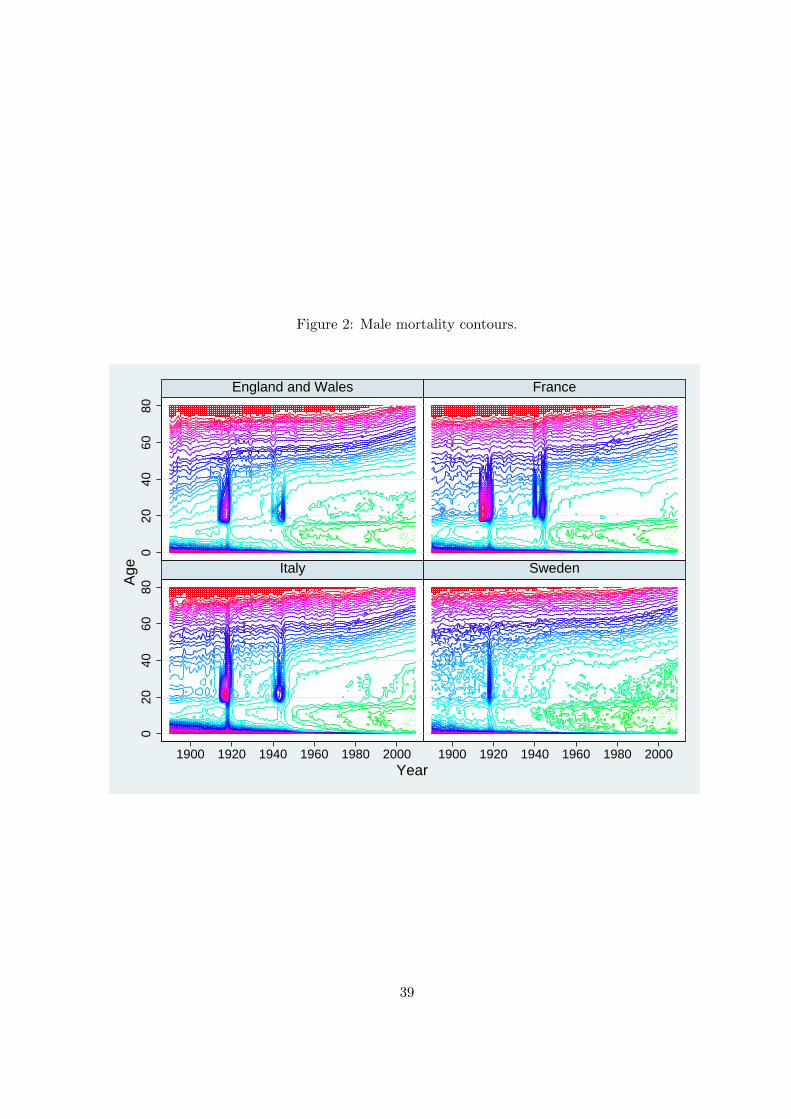
Figure 2: Male mortality contours.
020
4060
800
2040
6080
1900 1920 1940 1960 1980 2000 1900 1920 1940 1960 1980 2000
England and Wales France
Italy Sweden
Age
Year
39

Figure 3: Percent reporting stress.
01
23
01
23
01
23
01
23
1935 1945 1955 1965
Austria Belgium Czech Rep Denmark
France Germany Greece Italy
Netherlands Poland Spain Sweden
Switzerland
Per
cent
Year
40

Figure 4: Distribution of the year when stress started and ended.
050
100
050
100
050
100
1935 1945 1955 1965 1935 1945 1955 1965 1935 1945 1955 1965
Austria Belgium France
Germany Greece Italy
Netherlands Poland Spain
Started Ended
Per
cent
Year
41

Figure 5: Percent reporting absence of the parents at age 10.
015
3045
015
3045
015
3045
015
3045
1935 1945 1955 1965
Austria Belgium Czech Rep Denmark
France Germany Greece Italy
Netherlands Poland Spain Sweden
Switzerland
Mother Father
Per
cent
Year
42

Figure 6: Percent reporting financial hardship.
05
100
510
05
100
510
1935 1945 1955 1965
Austria Belgium Czech Rep Denmark
France Germany Greece Italy
Netherlands Poland Spain Sweden
Switzerland
Per
cent
Year
43

Figure 7: Distribution of the year when financial hardship started and ended.
050
100
050
100
050
100
1935 1945 1955 1965 1935 1945 1955 1965 1935 1945 1955 1965
Austria Belgium France
Germany Greece Italy
Netherlands Poland Spain
Started Ended
Per
cent
Year
44

Figure 8: Percent reporting hunger.
010
200
1020
010
200
1020
1935 1945 1955 1965
Austria Belgium Czech Rep Denmark
France Germany Greece Italy
Netherlands Poland Spain Sweden
Switzerland
Per
cent
Year
45

Figure 9: Distribution of the year when hunger started and ended.
050
100
050
100
050
100
1935 1945 1955 1965 1935 1945 1955 1965 1935 1945 1955 1965
Austria Belgium France
Germany Greece Italy
Netherlands Poland Spain
Started Ended
Per
cent
Year
46

Figure 10: Geography of hunger and war.
20 - 5018 - 2015 - 1813 - 1510 - 137.5 - 105 - 7.52.5 - 50 - 2.5No data
Percent reporting hunger, born 1930-3920 - 5018 - 2015 - 1813 - 1510 - 137.5 - 105 - 7.52.5 - 50 - 2.5No data
Percent reporting hunger, born 1940-49
No war
1 year
2 years
3+ years
No data
Regions affected by war operations 1936-45
47

Figure 11: Distribution of the year when first witnessed war or experienced financial hardship.
050
100
Per
cent
1935 1945 1955 1965Year
Witnessed war Financial hardship
48

Figure 12: Fraction of migrants by country and year
05
1015
05
1015
05
1015
05
1015
1930 1935 1940 1945 1950 1955 1930 1935 1940 1945 1950 1955 1930 1935 1940 1945 1950 1955
1930 1935 1940 1945 1950 1955
Austria Belgium Czech Rep Denmark
France Germany Greece Italy
Netherlands Poland Spain Sweden
Switzerland
Per
cent
age
Year
49

A Details on SHARE and ELSA
This appendix provides some detail on the temporal and spatial information provided by SHARE
and ELSA, and the information on childhood health and SES, hardship episodes in childhood, and
adult outcomes.
A.1 Temporal and spatial information
A key feature of the public use version of SHARELIFE is the possibility of determining the country,
region and area in which an individual was living in any given year. The basic information comes
from Module AC (Accommodation), which collects information on the different places an individual
lived in during her life. The module begins with a question on the residence the respondent lived
in when was born, where by residence is meant an apartment or single house. It then collects
information on each other residence the respondent lived in for more than 6 months, including the
year the person started and stopped living at that residence, the country (at current boundaries),
the region (at different level of geographically detail depending on the country) and the area of
residence (big city, suburbs or outskirts of a big city, large town, small town, rural area or village).
As for the country of residence, two questions are asked. First, for each past residence the
survey instrument asks whether it was within the current boundaries of the country in which the
respondent is currently living. If the answer is no, a second question is asked using a showcard:
Which country, considering current boundaries, was this residence in? The showcard reports the
names of the main European countries, Russia, the USA, and two residual categories, namely other
European country and other non-European country. The region of residence is asked only if the
country of past residence coincides with that of current residence. This means that the region
of residence cannot be determined for those who in a given year have changed their country of
residence.
Since we know the starting and ending year and the country/region/area of each residency,
we are able to construct a longitudinal data set with annual observations for each individual. An
important problem is the fact that the level of regional disaggregation in SHARELIFE varies by
country: it is at the coarse NUTS1 level for Belgium, Denmark, France and the Netherlands, at
the fine NUTS3 level for the Czech Republic, and at the intermediate but not very detailed NUTS2
level for Austria, Germany, Greece, Italy, Poland, Spain, Sweden and Switzerland.
Unlike SHARELIFE, the public use version of ELSALIFE contains little information on past
residence and no information that can be used to determine the country and region of residence in
50

a given year. Basically, we can only determine whether the respondent was living in the U.K. or
abroad in a given year.
A.2 SES and health in childhood
Module CS (Childhood SES) of SHARELIFE collects information on the occupation of the main
breadwinner (white collar, blue collar, farmer, etc.), the number of books at home, features of
the accommodation (presence of fixed bath, running water, inside toilet, central heating, number
of rooms available), the number of people living in the house when the respondent was aged 10,
and whether parents, siblings and grandparents were living in the house when the respondent was
aged 10. Module HS (Health status) of SHARELIFE contains information on both the self-reported
health status in childhood (age 0–15) as well as experiences of distinct illnesses during childhood
(infectious diseases, polio, asthma, allergies, heart trouble, etc.). Then, for each illness, it is asked
the age-interval when it was experienced: between age 0–5, 6–10, 11–15. We construct a measure
of childhood health that counts the number of chronic illnesses respondents experienced in the
age interval 6–15, considering the following diseases: polio, asthma, allergies (other than asthma),
epilepsy, psychiatric problems, diabetes, heart trouble, leukaemia or lymphoma and cancer.
ELSALIFE asks comparable questions regarding the number of books at home, features of
the accommodation, the presence of distinct members of the family (all measured with reference
to age 10) and health status in childhood. However, there are some differences with respect to
SHARELIFE. In particular, ELSALIFE does not collect information on the occupation of the main
breadwinner when the respondent was aged 10, but rather on the occupation of the father when
the respondent was aged 14. Further, it does not include questions on the specific timing of the
illnesses experienced during childhood. As for health status in childhood, we use a self-reported
health measure, namely an indicator for being in fair or poor health.
A.3 Hardship episodes in childhood
Module GL (General Life) of SHARELIFE collects information on the experience of hardship
episodes. This section first asks: Looking back on your life, was there a distinct period during
which you were under more stress compared to the rest of your life? If the answer is yes, it asks
When did this period start?, followed by When did this period stop? It then asks similar questions
for poor health (Looking back on your life, was there a distinct period during which your health
was poor compared to the rest of your life?), financial hardship (Looking back on your life, was
there a distinct period of financial hardship?), and hunger (Looking back on your life, was there a
51

distinct period during which you suffered from hunger?). The formulation of these questions allows
to determine the duration of the reported hardship episode, defined as the difference between the
year when they ended and the year when they started, although we have no other information
on their intensity. Notice that respondents are asked to report only one episode for each type of
hardship, presumably the most salient (phrases such as “distinct period” or “compared to the rest
of your life” are meant to capture this idea). Also notice that there may be heterogeneity in the
perception of each hardship across individuals, which raises the issue of interpersonal comparability.
Unlike SHARELIFE, ELSALIFE gathers direct information on having witnessed serious injury
or death of someone in war or military action, and having been evacuated during WW2. Specifically,
the survey instrument asks: Have you ever witnessed the serious injury or death of someone in war
or military action? If the answer is yes, it then asks: How old were you when it first happened?
The next question is directly about WW2: Have you ever been evacuated during World War II?
As with SHARELIFE, ELSALIFE also gathers information on having experienced severe fi-
nancial hardship and on the family’s SES around age 10. Specifically, the survey instrument asks:
Have you ever experienced severe financial hardship?. If the answer is yes, the interviewee is then
asked: How old were you when it first happened?.
As for the family’s SES around age 10, ELSALIFE includes questions that are very similar to
those in SHARE, such as the number of books at home, accommodation features, the job of the
main breadwinner, whether distinct members of the family were present in the house at the age
of 10. The latter question is used to infer information on the absence of the father and the mother.
Notice that financial hardship and absence of the father at age 10 are the only hardship episodes
directly comparable with those recorded in SHARE. Further, we only know the age when financial
hardship started, not its duration. This means that we can only estimate the long-term effects of
financial hardship episodes that started at a given age, not of financial hardship experienced at
different ages.
A.4 Adult outcomes
The adult outcomes that we consider are all collected in the regular waves of SHARE and ELSA.
Some of these outcomes are directly comparable between the two surveys, but others are not.
The comparable outcomes are SRH, the test of memory (recall), life satisfaction and happiness.
SRH is defined on a 1–5 scale for both surveys with a slight difference in the definition of the
categories (for SHARE the available categories are “excellent”, “very good”, “good”, “fair”, “poor”,
52

whereas for ELSA the available categories are “very good”, “good”, “fair”, “bad” and “very bad”).
For both SHARE and ELSA, the memory test consists of verbal registration and recall of a list of
10 words, carried out twice, first immediately after the encoding phase (immediate recall) and then
some 5 minutes later (delayed recall). Our measure of recall is the sum of the scores on immediate
and delayed recall, which ranges from a minimum of 0 to a maximum of 20. The numeracy test
in SHARE consists of five questions involving simple arithmetical calculations based on real life
situations and the test score ranges from a minimum of 1 to a maximum of 5. In ELSA, instead,
the numeracy test was only administered in wave 1. As for life satisfaction, the precise wording of
the question and its scale are different between the two surveys. SHARE respondents are asked
to choose a value between 0 and 10, with 0 meaning “completely dissatisfied” and 10 meaning
“completely dissatisfied”, while ELSA respondents are asked to choose a value between 1 and 7,
with 1 meaning “strongly agree” and 7 meaning “strongly disagree”. Happiness is instead defined
in the same way in both surveys.
Important differences between SHARE and ELSA arise for BMI, education and depression.
As for BMI, height and weight are self-reported in SHARE, while in ELSA they are objectively
measured during the nurse visit. As for education, ELSA does not ask the number of years of
completed schooling but instead the age at which the respondent left full time education. As for
depression, SHARE uses the Euro-D index, which summarizes a series of conditions related to
mental health (depression, anxiety, suicidality, etc.), while ELSA only asks whether the respondent
was feeling depressed in the past week.
53

B Additional tables
Table B1: Survival rates up to year 2006 by birth cohort and country. Females.
CountryBirth cohort BE CH DK ES EW FR IT NL SW
1918 .229 .298 .217 .229 .221 .291 .244 .239 .2681919 .292 .342 .258 .273 .269 .360 .315 .295 .3231920 .282 .371 .277 .293 .264 .360 .293 .319 .3481921 .360 .441 .327 .352 .326 .428 .378 .375 .4101922 .399 .478 .358 .393 .362 .466 .403 .415 .4421923 .449 .525 .396 .439 .401 .511 .456 .460 .4921924 .485 .564 .428 .480 .434 .544 .485 .499 .5281925 .520 .609 .463 .516 .472 .580 .524 .532 .5701926 .562 .635 .489 .554 .504 .617 .559 .569 .6051927 .591 .665 .520 .584 .540 .642 .592 .603 .6291928 .624 .694 .552 .618 .575 .668 .622 .630 .6711929 .655 .720 .577 .638 .612 .698 .655 .663 .6941930 .686 .745 .603 .663 .641 .721 .678 .689 .7171931 .710 .763 .629 .691 .671 .739 .702 .712 .7381932 .734 .783 .657 .720 .703 .761 .731 .737 .7571933 .759 .800 .682 .738 .730 .779 .746 .760 .7791934 .774 .815 .704 .758 .754 .795 .761 .782 .7971935 .790 .828 .730 .772 .773 .809 .782 .796 .8101936 .807 .845 .755 .778 .793 .823 .787 .816 .8261937 .821 .856 .782 .792 .812 .836 .811 .828 .8471938 .831 .864 .798 .810 .825 .846 .820 .839 .8561939 .840 .872 .816 .837 .838 .852 .837 .849 .8661940 .852 .883 .833 .824 .851 .862 .843 .861 .8731941 .862 .893 .847 .849 .870 .879 .853 .869 .8911942 .871 .899 .857 .874 .880 .880 .865 .876 .8921943 .881 .902 .867 .875 .890 .889 .875 .886 .9021944 .887 .913 .875 .886 .900 .892 .879 .892 .9081945 .897 .919 .893 .894 .909 .905 .891 .903 .9191946 .908 .927 .896 .905 .920 .913 .906 .919 .9231947 .916 .932 .911 .916 .920 .922 .915 .923 .9311948 .920 .936 .919 .916 .931 .926 .923 .928 .9371949 .926 .942 .923 .923 .937 .931 .930 .932 .9421950 .931 .947 .927 .930 .940 .934 .936 .937 .9451951 .935 .949 .933 .937 .945 .938 .941 .941 .9501952 .939 .954 .939 .944 .950 .942 .947 .945 .9551953 .944 .957 .943 .946 .953 .946 .952 .949 .9571954 .949 .959 .946 .952 .956 .949 .955 .952 .9601955 .953 .962 .953 .956 .961 .953 .959 .955 .9651956 .957 .964 .955 .958 .963 .955 .961 .958 .967
54

Table B2: Survival rates up to year 2006 by birth cohort and country. Males.
CountryBirth cohort BE CH DK ES EW FR IT NL SW
1918 .086 .133 .089 .100 .090 .103 .098 .083 .1181919 .120 .158 .110 .129 .126 .148 .139 .115 .1601920 .112 .178 .126 .142 .117 .143 .118 .125 .1691921 .164 .232 .161 .174 .163 .199 .179 .171 .2231922 .195 .263 .185 .202 .191 .228 .194 .200 .2511923 .230 .303 .217 .242 .225 .262 .235 .233 .3011924 .263 .335 .259 .276 .253 .292 .259 .268 .3371925 .298 .382 .293 .312 .292 .326 .297 .304 .3761926 .333 .421 .326 .351 .326 .364 .337 .346 .4101927 .371 .452 .364 .378 .371 .392 .376 .388 .4481928 .405 .491 .397 .420 .414 .423 .408 .423 .4881929 .446 .528 .437 .446 .459 .459 .455 .466 .5241930 .485 .556 .472 .477 .498 .488 .485 .504 .5541931 .517 .590 .495 .507 .533 .514 .518 .536 .5861932 .553 .621 .529 .546 .570 .547 .558 .578 .6171933 .584 .655 .560 .566 .606 .574 .584 .608 .6461934 .621 .675 .596 .598 .639 .601 .607 .642 .6711935 .644 .696 .629 .621 .664 .628 .643 .670 .6981936 .671 .720 .661 .629 .693 .653 .660 .698 .7211937 .697 .745 .690 .650 .719 .677 .693 .722 .7471938 .717 .764 .713 .685 .741 .695 .712 .745 .7701939 .735 .777 .737 .729 .757 .714 .737 .764 .7861940 .745 .797 .752 .708 .775 .732 .751 .785 .7971941 .769 .813 .777 .741 .803 .762 .768 .801 .8231942 .781 .824 .790 .782 .817 .768 .788 .815 .8331943 .794 .839 .806 .782 .832 .781 .800 .827 .8451944 .808 .846 .820 .794 .848 .792 .811 .839 .8571945 .827 .861 .832 .812 .861 .810 .831 .854 .8701946 .840 .872 .849 .826 .880 .824 .851 .879 .8791947 .850 .877 .863 .848 .882 .837 .864 .885 .8891948 .865 .887 .869 .845 .896 .847 .877 .895 .8971949 .876 .892 .877 .860 .903 .857 .888 .901 .9031950 .882 .899 .882 .873 .908 .863 .897 .908 .9121951 .887 .906 .891 .884 .915 .870 .903 .915 .9181952 .897 .914 .895 .892 .920 .879 .912 .921 .9221953 .901 .918 .900 .899 .925 .885 .919 .927 .9261954 .909 .921 .906 .906 .931 .892 .924 .930 .9321955 .916 .925 .915 .912 .936 .897 .927 .935 .9371956 .922 .929 .919 .917 .941 .903 .931 .940 .942
55