Growth Accounting with Demand Instability andIncome Effects

David R. Baqaee

UCLA

Ariel Burstein∗

UCLA

April 22, 2021

Abstract

We study how welfare responds to changes in budget and production possibility

sets when preferences are unstable or non-homothetic. We characterize the gap be-

tween welfare and standard measures of real consumption in partial and general equi-

librium. We show that measures of real consumption are biased whenever changes

in expenditures due to income effects or demand instability covary with changes in

prices. This bias appears because real consumption does not properly account for

consumer substitution. We apply our results to long-run and short-run phenomena.

In the long-run, we show that structural transformation, if caused by income effects,

has much larger implications for welfare than what is implied by standard measures

of Baumol’s cost disease. In the short-run, we show that when firms’ demand shocks

are correlated with their supply shocks, industry-level price and output indices are

biased, and this bias does not disappear in the aggregate. Finally, we show that corre-

lated supply and demand shifters make real GDP and aggregate TFP unreliable met-

rics for measuring production and productivity, and illustrate this using the Covid-19

crisis.

∗We thank Sihwan Yang for superb research assistance. We thank Andy Atkeson, Natalie Bau, and JonVogel for helpful comments. We are grateful to Emmanuel Farhi and Seamus Hogan, both of whom passedaway tragically before this paper was written, for their insights and earlier conversations on these topics.This paper received support from NSF grant No. 1947611.

1 Introduction

How does a change in the economic environment affect welfare? For example, how doesthe welfare of a consumer change when the budget constraint changes, or how doesthe welfare of a nation change when the production possibility frontier of the economychanges? At first blush, answering this question seems very difficult, perhaps requiringdetailed information about the nonlinear functions describing preferences and technolo-gies.

Under the strong assumptions of homotheticity and preference stability, standard the-ory offers a simple non-parametric procedure for recovering the answer to these ques-tions. Consider a change in prices and income that occurred over some time horizon t0 tot1. Indexing individual goods by i, the change in welfare is approximately equal to

∆Welfare ≈ ∆ log I −t1

∑t=t0

∑i

bi(t) (log pi(t + 1)− log pi(t)) , (1)

where ∆ log I is the log change in nominal income, and bi(t) and pi(t) are the budgetshare and price of good i at time t. In words, the change in nominal income deflated bythe expenditure-share weighted change in prices approximates the change in welfare. Thefact that the expenditure shares are updated at every period t between t0 and t1 reducessubstitution bias, and eliminates it in the continuous-time limit.

Equation (1) is a chain-linked index, and such indices are used to measure most typesof real economic activity, ranging from aggregates like real GDP, total factor productivity(TFP), private consumption and investment, to less aggregated objects like industry-levelmeasures of inflation and production. The fact that these indices approximate changesin welfare and production under homotheticity and stability justifies their recommendeduse in the United Nations’ System of National Accounts.1

While homotheticity and preference stability are highly convenient assumptions, theyhave counterfactual implications: homotheticity requires that income effects be uniform,that is, the income elasticity of demand must equal one for every good; stability requiresthat consumers only change their spending decisions in response to changes in incomesand relative prices. In this paper, we provide sufficient statistics that adjust equation (1)when these assumptions are relaxed.2 Our baseline welfare measure is the equivalent

1See OECD et al. (2004) and references therein, in particular Chapters 15 and 17, for a comprehensiveoverview and discussion of price and quantity indices and their relation to welfare.

2As we discuss in detail in Section 2, preference instability is driven by any factor that changes preferencerankings over bundles of goods at fixed prices and income, e.g. age, health, advertising, fads. In theliterature, preference instability and non-homotheticities are typically studied independently. We analyze

1

variation at fixed final preferences, which answers the question: “holding fixed prices andpreferences, how much income must consumers be given to make them indifferent between theirchoice sets at t0 and t1?”

We study this problem in both partial equilibrium, where choice sets are defined interms of budget sets (prices and income are exogenous), and in general equilibrium,where choice sets are defined in terms of production possibility frontiers (prices andincome are endogenous).3 We provide exact and approximate characterizations of theadjustment to equation (1), and demonstrate that the failure of chain-linked indices, inboth partial and general equilibrium, is caused by the fact that they undermeasure thesubstitution caused by either income effects or preference instability. That is, with non-homotheticities or preference instability, chained indices, like real consumption, real GDP,or TFP, suffer from exactly the type of substitution bias that they were designed to elim-inate. We show that this bias is larger if changes in expenditures caused by income ef-fects or taste shocks are correlated with changes in prices. If, on the other hand, demandshifters are uncorrelated with price changes (or, in general equilibrium, if demand shiftersare orthogonal to supply shifters), then no adjustment is required and (1) holds.

Our partial equilibrium welfare measure answers a microeconomic question for aninfinitesimal agent who cannot alter market-level prices through her choices. Our gen-eral equilibrium welfare measure answers a macroeconomic question for a collection ofagents whose collective decisions alter market-level prices. When preferences are stable,macroeconomic changes in welfare are equal to microeconomic changes in welfare. How-ever, we show that these two measures are not equal when household preferences changeover time. Intuitively, some points on a budget constraint, which may be feasible for anindividual agent, are not feasible for society as a whole due to curvature in the productionpossibility frontier.

Our results for welfare and the gap between welfare and real consumption are ex-pressed in terms of measurable sufficient statistics. Surprisingly, in both partial and gen-eral equilibrium, we show that computing the change in welfare caused by changes inprices (in partial equilibrium) or technology (in general equilibrium) does not require di-rect knowledge of the taste shocks or the shape of non-homotheticities. Instead, whatwe must know are the expenditure shares and the elasticities of substitution at the finalallocation. For the micro problem, these are the household expenditure shares and theelasticities of substitution in consumption. For the macro problem, these are the input-

them jointly in this paper because both generate the same type of biases in measures of real consumption.Our results are relevant when either of these forces is active.

3For the macro problem, we consider neoclassical economies with representative agents.

2

output table and the elasticities of substitution in both production and consumption.In general equilibrium, for very simple economies with one factor and no interme-

diates, the difference between welfare and real GDP is approximately half the covari-ance of supply and demand shocks. This formula can be generalized to more complexeconomies. We show how the details of the production structure, like input-output link-ages, complementarities in production, and decreasing returns to scale, interact with non-homotheticities and preference shocks to magnify the gap between welfare and GDP.There is no reason to expect the discrepancies between welfare and GDP that we empha-size to get aggregated away. In fact, these discrepancies can become larger the more wedisaggregate. In this sense, our results are related to the literature studying the macroeco-nomic implications of production networks and disaggregation (e.g. Gabaix, 2011; Ace-moglu et al., 2012; Baqaee and Farhi, 2019c).

We illustrate the relevance of our results for understanding short-run and long-runphenomena by means of three applications. In our first application, we analyze the im-portance of non-homotheticity or preference instability for measures of long-run produc-tivity growth. Since Baumol (1967), an enduring stylized fact about economic growth hasbeen the observation that industries with slow productivity growth tend to become largeras a share of the economy over time. This phenomenon, known as Baumol’s cost disease,implies that aggregate growth is increasingly determined by productivity growth in slow-growth industries since, over time, the industrial mix of the economy shifts to favor theseindustries. To be specific, from 1948 to 2014, aggregate TFP in the US grew by 60%. If theUS economy had kept its original 1948 industrial structure, then aggregate TFP wouldhave grown by 78% instead. We show that if structural transformation is caused solely bynon-homotheticity and demand instability, then welfare-relevant TFP grew by only 47%.This is because measured aggregate TFP does not fully account for substitution caused bychanges in demand, and hence, the increase in the welfare-relevant measure of aggregateTFP is much lower than what is measured.

In our second application, we consider a firm-level specification of our model. Weshow that when firms’ demand shocks are correlated with their supply shocks, there is agap between welfare-relevant and measured changes in industry-level output and prices.We show that these biases, which can be sizable even at annual frequency, do not disap-pear as we aggregate up to the level of real GDP even if firms and industries are infinites-imal. At annual frequency, the gap between welfare and real GDP due only to firm-levelsupply and demand shocks could be as high as 1%, and this gap gets larger at lowerfrequencies if firm-level supply and demand shocks are persistent, becoming unbound-edly large in the limit when the shocks are random walks. If we start with industry-level

3

(rather than firm-level) data, we are ruling out the existence of these biases by construc-tion.4

In our final application, we show that if changes in household spending patterns are inpart driven by demand shifters, then real GDP and aggregate TFP can become unreliablemetrics for measuring changes in production and productivity. What should be irrelevantdetails, like the order of supply and demand shocks, can cause real GDP to be differentbetween the initial and final periods even if initial and final prices and quantities are thesame. To illustrate these results, we consider the large changes in household spendingpatterns towards low-contact goods and services over the first few months of 2020 dueto the Covid-19 pandemic. Since these changes in spending patterns were not entirelydriven by market prices, real GDP is path dependent. For example, if the path of supplyand demand shocks during the recovery does not look exactly like the initial collapse inreverse, measured real GDP can be as much as 6% higher or lower than what it was beforethe crisis, even if every price and quantity returns to its pre-Covid value.

Of course, there are other reasons, besides instability and non-homotheticity, why (1)can fail to accurately measure welfare. Many of the well-known reasons why the approx-imation in (1) fails can be thought of as being due to missing prices and quantities. Forexample, it is well-known that (1) fails to properly account for the creation and destruc-tion of goods if we cannot measure the quantity of goods continuously as their price fallsfrom or goes to their choke price (Hicks, 1940; Feenstra, 1994; Hausman, 1996; Aghionet al., 2019); equation (1) also fails to properly account for changes in the quality of goods(see Syverson, 2017); finally, (1) fails to properly account for changes in non-market com-ponents of welfare, like changes in leisure and mortality (see Jones and Klenow, 2016),or changes in the user cost of durables. In all of these cases, the problem is that some ofthe relevant prices or quantities in the consumption bundle are missing or mismeasured,and correcting the index involves imputing a value for these missing prices or quanti-ties. In this paper, we abstract from these issues and assume that prices and quantitieshave been correctly measured. If prices and quantities are mismeasured or missing, thenour results would apply to the quality-adjusted, corrected, version of prices instead ofobserved prices. That is, the corrections we derive are different to the ones that are equiv-alent to adjustments in prices.5

4These aggregation biases are not unique to firm-level data, a similar logic also applies to the use ofsectoral aggregates in place of more disaggregated industry-level data, whereby sectoral measures of TFPare contaminated by substitution bias caused by demand instability and income effects.

5Our approach to calculate ex-post welfare changes requires well-measured prices and elasticities ofsubstitution in the final period. For ex-post welfare measurement, when information on prices is missingor mismeasured, if preferences are non-homothetic an alternative approach is to infer changes in welfareby relying on changes in prices, expenditures, price elasticities, and Engel curve slopes for only a subset of

4

Relatedly, preference instability and mismeasured prices (i.e. unobserved quality change)are sometimes viewed as alternative means to the same end. This is because they can bothbe used to justify why demand curves shift over time, even holding prices and incomesfixed. That is, both can rationalize changes in behavior that are not triggered by changesin observed prices or incomes. However, while they have similar implications for changesin prices and quantities, they have very different implications for welfare. When there areunobserved changes in quality, the gap between welfare and real consumption is causedby a difference between measured and welfare-relevant prices. We show that in the caseof non-homotheticities and taste shocks, the gap between welfare and real consumptionis caused by a difference between measured and welfare-relevant expenditure shares.

Other related literature. This paper contributes to the literatures on growth and pro-ductivity accounting, multi-sectoral and disaggregated macroeconomics, as well as theliterature on structural transformation. We discuss the way our paper complements andrelates to these literatures in turn.

A key assumption in growth accounting is the existence of a stable and homotheticfinal aggregator. As shown by, for example Hulten (1973) among others, chain-linked in-dices are meaningful if, and only if, a homothetic and stable final aggregator exists. There-fore, this assumption is ubiquitous in growth accounting, and also appears in almost allpapers that study aggregate outcomes using disaggregated input-output models.6 Weshow that when preferences are non-homothetic or unstable, then the “ideal” price de-flator is shock-dependent. This allows us to provide a generalization of Domar (1961)and Hulten (1978) that measures changes in welfare in situations when preferences areunstable or non-homothetic. Using this, we can construct exact and approximate charac-terizations of how welfare responds to shocks in general equilibrium, a question which isof central importance in the literature on disaggregated and production network models.7

Our approach contrasts with the one in Redding and Weinstein (2020). They show thatvariations in sales are difficult to explain via shifts in supply curves alone, and shifts indemand curves are an important source of variation in the data. They interpret changes

goods, given assumptions on separability and stability in preferences (see e.g. Hamilton, 2001 and, morerecently, Atkin et al., 2020). In addition to ex-post measurement with non-homotheticities, in this paperwe study the implications of instability of preferences (that generate shifts in expenditures correlated withprice changes) and we also consider counterfactuals.

6See, for example, the review paper by Carvalho and Tahbaz-Salehi (2018) and the references therein.7The biases we identify, and the failure of Hulten’s theorem, are not caused by inefficiencies (e.g.

markups, wedges, taxes). Baqaee and Farhi (2019b) analyze how growth accounting must be adjusted ininefficient economies. Whereas incorporating inefficiencies in production does not affect our micro welfareresults, how they interact with demand instability and non-homotheticity in general equilibrium is beyondthe scope of this paper.

5

in demand curves as being due to changes in tastes, but unlike us, they treat changes intastes as being equivalent to changes in price. Operationally, this makes the taste shocksbehave like quality shocks. They estimate changes in taste/quality necessary to explainvariations in product-level data. However, this only determines changes in the relativesize of demand shocks across goods, and it does not pin down changes in the overalllevel of these shocks. Redding and Weinstein (2020) pin down the overall level of theshocks by assuming they are mean zero. They then derive CES price indices for changesin utility in the presence of such shocks. Our approach is different in that we do notcompare utils before and after the taste shocks. Instead we compute changes in equiv-alent variation keeping preferences over goods constant for the variation, as advocatedby Fisher and Shell (1968) and Samuelson and Swamy (1974). This approach does notrequire any assumptions about the overall level of the taste shocks in terms of utils.8

Our paper is also related to the literature on structural transformation and Baumol’scost disease. As explained by Buera and Kaboski (2009) and Herrendorf et al. (2013), thisliterature advances two microfoundations for structural transformation. The first expla-nation is all about relative prices differences: if demand curves are not unit-price-elastic,then changes in relative prices change expenditure shares (e.g. Ngai and Pissarides, 2007;Acemoglu and Guerrieri, 2008; Buera et al., 2015). The second explanation emphasizesnon-homotheticities, or income effects, whereby households spend more of their incomeon some goods as they become richer (e.g. Kongsamut et al., 2001; Boppart, 2014; Cominet al., 2015; Alder et al., 2019).

Our results suggest that settling this question has important implications for welfare.From a welfare perspective, structural transformation driven by relative price changesshould be treated differently to structural transformation driven by non-homotheticityor demand instability. In particular, measures of real production or consumption mustbe adjusted for substitution bias in the latter case, but no adjustment is necessary in theformer case.

The structure of the paper is as follows. In Section 2, we set up the microeconomicproblem and provide exact and approximate characterizations of the difference betweenwelfare and measured real consumption changes. In Section 3, we set up the macroeco-

8Some papers in index number theory have studied the relationship between conventional index num-bers and welfare in the presence of preference instability and non-homotheticities. For example, Caveset al. (1982) show that when preferences are homothetic, translog, but unstable, measured Tornqvist-basedindices correspond to a geometric average of welfare changes under initial and final preferences. A similarresult holds in our context, as we show in Appendix B, but in the body of the paper our focus is different.We characterize welfare (in partial and general equilibrium) at either initial or final preferences and usingeither EV or CV, rather than averaging these different measures.

6

nomic general equilibrium model and provide exact and approximate characterizationsof the difference between welfare and measured real output changes. Whereas in section3 we present our macro results in terms of endogenous sufficient statistics, in Section 4we solve for these endogenous sufficient statistics in terms of microeconomic primitivesand consider some simple but instructive analytical examples. Our applications are inSection 5. We discuss some extensions in Section 6 and conclude in Section 7. All proofsand additional details are in the appendix.

2 Microeconomic Changes in Welfare and Consumption

In this section, we consider changes in budget constraints in partial equilibrium. Weask how consumers value these changes, and compare these measures of welfare withmeasures of real consumption. We provide exact and approximate results. We model theequilibrium determination of prices in Section 3.

2.1 Definition of Welfare and Real Consumption

In this subsection we define welfare and real consumption. Measuring changes in welfareusing equivalent variation is standard when preferences are stable. However, measuringwelfare changes in the presence of unstable preferences is less common and therefore wediscuss this issue in some detail.

Consider a set of preference relations, x, over bundles of goods. These preferencesare indexed by x, which represents anything that affects preference rankings over bundlesof goods. For example, x could be calendar time, age, exposure to advertising, or state ofnature. For every x, we represent the preference relation x by a utility function u(c; x),where c ∈ RN and N is the number of goods in the consumption bundle. Since theconsumer makes no choices over x, we do not need to specify how u(c; x) varies with x.Moreover, preferences over x, if they exist, are not revealed by choices.9

There are two properties of preferences that are analytically convenient benchmarksthroughout the rest of the analysis.

Definition 1 (Homotheticity). Preferences over goods c are homothetic if, for every positive

9In Section 6, we discuss situations in which x is endogenously chosen and valued by the consumer,such as leisure, but its price and quantity are not being measured. We also discuss situations in which x isendogenously chosen by firms, such as advertising.

7

scalar a > 0 and every feasible c and x, we can write

u(ac; x) = au(c; x).

Definition 2 (Stability). Preferences over goods c are stable if there exists a time-invariantfunction Φ (·) such that the utility function can be written as u(c; x) = U(Φ(c); x) forevery feasible c and x.

If preferences are stable, x can change over time (e.g. households get higher or lower utilsfrom all goods) but, since x is separable from c, these changes do not impact preferencesover bundles of goods c. If preferences are not stable, we say that they are unstable.

Given preferences encapsulated in u, the indirect utility function of the consumer, forany value of x, is

v(p, I; x) = maxcu(c; x) : p · c = I.

where p is a price vector over goods and I is income. Consider shifts in the budget set asprices and income change from pt0 and It0 to pt1 and It1 . This change in the budget set isaccompanied by changes in x from xt0 to xt1 . Our baseline measure of welfare is definedas follows.

Definition 3 (Micro Welfare). The change in welfare measured using the micro equivalentvariation with final preferences is EVm(pt0 , It0 , pt1 , It1 ; xt1) = φ where φ solves

v(pt1 , It1 ; xt1) = v(pt0 , eφ It0 ; xt1). (2)

In words, EVm is the change in income (in logs), under initial prices pt0 , that a con-sumer with preferencesxt1

would need to be indifferent between the budget set definedby initial prices (pt0 , eφ It0) and the new budget set defined by new prices and income(pt1 , It1).

10 The new budget set is preferred to the initial one, if and only if, EVm is posi-tive. The superscript m represents the fact that this is the micro equivalent variation, sincewe take prices as given.

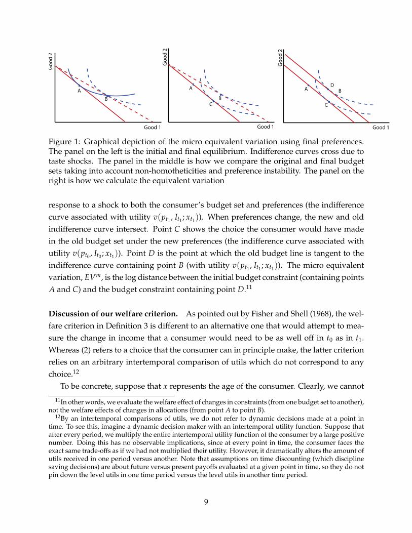
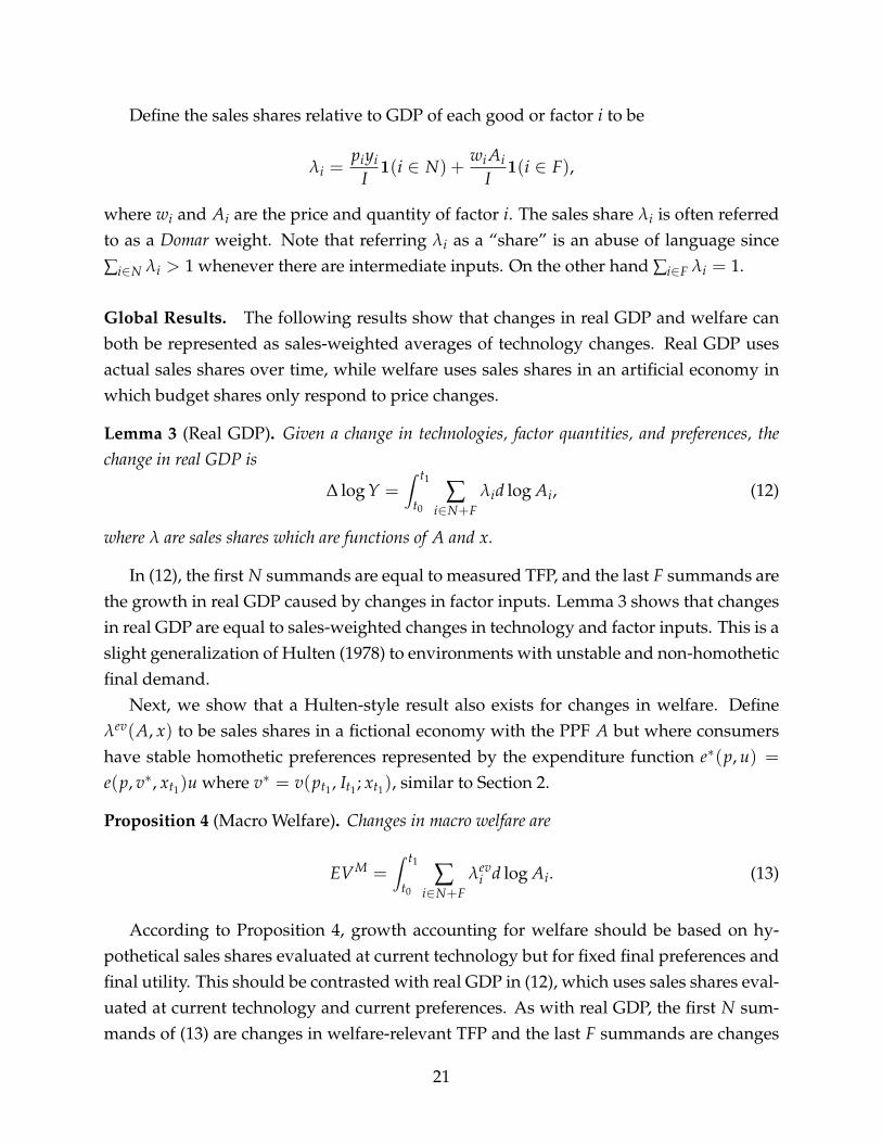
Figure 1 illustrates EVm in a simple two good economy. Point A depicts the con-sumer’s choice at some initial equilibrium. Point B shows the consumer’s new choice in

10In principle, we could also measure changes in welfare using compensating (instead of equivalent)variation, or by using initial (rather than final) preferences (see e.g. Balk, 1989 for a discussion of the variousways one can define welfare changes). Combining EV with final preferences (CV with initial preferences)is natural since this requires preserving the shape of the indifference curve at the final (initial) allocation. Inthe body of the paper, for conciseness, we focus on EV using final preferences since equivalent variation ismore commonly used and final preferences are more relevant than initial preferences, but we characterizethese other welfare measures in Appendix B. See also Remark 1.

8

A

C

Good 1

Go

od

2

BA

Good 1

Go

od

2

B

A

C

Good 1

Go

od

2

B

D

Figure 1: Graphical depiction of the micro equivalent variation using final preferences.The panel on the left is the initial and final equilibrium. Indifference curves cross due totaste shocks. The panel in the middle is how we compare the original and final budgetsets taking into account non-homotheticities and preference instability. The panel on theright is how we calculate the equivalent variation

response to a shock to both the consumer’s budget set and preferences (the indifferencecurve associated with utility v(pt1 , It1 ; xt1)). When preferences change, the new and oldindifference curve intersect. Point C shows the choice the consumer would have madein the old budget set under the new preferences (the indifference curve associated withutility v(pt0 , It0 ; xt1)). Point D is the point at which the old budget line is tangent to theindifference curve containing point B (with utility v(pt1 , It1 ; xt1)). The micro equivalentvariation, EVm, is the log distance between the initial budget constraint (containing pointsA and C) and the budget constraint containing point D.11

Discussion of our welfare criterion. As pointed out by Fisher and Shell (1968), the wel-fare criterion in Definition 3 is different to an alternative one that would attempt to mea-sure the change in income that a consumer would need to be as well off in t0 as in t1.Whereas (2) refers to a choice that the consumer can in principle make, the latter criterionrelies on an arbitrary intertemporal comparison of utils which do not correspond to anychoice.12

To be concrete, suppose that x represents the age of the consumer. Clearly, we cannot

11In other words, we evaluate the welfare effect of changes in constraints (from one budget set to another),not the welfare effects of changes in allocations (from point A to point B).

12By an intertemporal comparisons of utils, we do not refer to dynamic decisions made at a point intime. To see this, imagine a dynamic decision maker with an intertemporal utility function. Suppose thatafter every period, we multiply the entire intertemporal utility function of the consumer by a large positivenumber. Doing this has no observable implications, since at every point in time, the consumer faces theexact same trade-offs as if we had not multiplied their utility. However, it dramatically alters the amount ofutils received in one period versus another. Note that assumptions on time discounting (which disciplinesaving decisions) are about future versus present payoffs evaluated at a given point in time, so they do notpin down the level utils in one time period versus the level utils in another time period.

9

meaningfully compare the amount of utils an individual derives from playing with toysduring childhood to the amount of utils that same individual derives from drinking wineduring adulthood. Since consumers never make choices about how old they are, theirpreferences across consumption goods consumed at different ages are not revealed bytheir choices. In the words of Heraclitus: “No man ever steps in the same river twice, forit’s not the same river and he’s not the same man.” A comparison of utils during child-hood to utils during adulthood is as meaningless as a comparison of utils between twodifferent individuals. On the other hand, if we fix the consumer’s age x, we can mean-ingfully compare the consumer’s preferences about the bundles of goods they consumedat different points in their life or different consumption streams that they may face in thefuture.

This approach, of holding x constant, is different to the one taken when x representssome form of quality change. Intuitively, quality adjustments are more applicable to sit-uations where the consumer can conceivably make choices between the good at differinglevels of quality. For example, if a box of chocolates undergoes quality change so that eachbox now contains twice as many chocolates, the consumer can conceivably make choicesbetween the old and new boxes that reveal how much they value the quality change. Tastechanges, on the other hand, do not involve meaningful choices from the consumer’s per-spective — if a consumer decides that she prefers dark chocolate to white chocolate, itdoes not make sense to ask how she would trade off consuming white chocolate in thepast, when she preferred white chocolate, to consuming dark chocolate in the present,when she prefers dark chocolate. Instead, holding fixed her preferences, we can ask howshe trades off white chocolate against dark chocolate. Therefore, the welfare implicationsof changes in unmeasured quality and changes in tastes are very different.

Of course, this is not to say that quality changes do not happen in reality. Rather, thatwe will abstract from quality change in our analysis. If there is quality change that can berepresented as an unobservable price reduction, then all of our results will apply to thequality-adjusted “correctly-measured” prices instead of the market prices.

Real Consumption. Having defined changes in welfare, we now define changes in realconsumption. The change in real consumption corresponds to what national income ac-countants and statistical agencies do when given data on the evolution of prices p andconsumption bundles c. We assume that this data is perfect — completely accurate, com-prehensive, adjusted for any necessary quality changes, and available in continuous time.This is because the biases associated with imperfections in the data, like the lack of qual-ity adjustment, missing prices, or infrequent measurement, are different to the biases we

10

study.

Definition 4 (Real consumption). For some continuously differentiable path of prices thatunfold as a function of some scalar t (interpreted as time), the change in real consumptionfrom t0 to t1 is defined to be

∆Y =∫ t1

t0∑i∈N

pi(t)dci

dtdt. (3)

That is, changes in real consumption are cumulated changes in consumption goodsmeasured at constant instantaneous prices.13 Equation (3) is called a Divisia quantity in-dex. In practice, since perfect data is not available in continuous time, statistical agenciesapproximate this integral via a (Riemann) sum using chained indices (e.g. Fisher or Torn-qvist). We abstract from the imperfections of these approximations in this paper.

In log terms, (3) can be rewritten as

∆ log Y =∫ t1

t0∑i∈N

bi(t)d log ci

dtdt =

∫ t1

t0∑i∈N

bid log ci, (4)

where bi(t) is the budget share of good i given prices, income, and preferences at timet. The last equation on the right-hand side simplifies notation by suppressing depen-dence on t in the integral. Using the budget constraint, we can express changes in realconsumption in terms of changes in income deflated by price changes,

∆ log Y = ∆ log I −∫ t1

t0∑i∈N

bid log pi = ∆ log I − ∆ log PY. (5)

In other words, changes in real consumption are equal to changes in income minus changesin the consumption price deflator. Notice that changes in real consumption (or the con-sumption price deflator) potentially depend on the entire path of prices and quantitiesbetween t0 and t1 and not just the initial and final values. This is unlike welfare changes,EVm, which depend only on initial and final prices and incomes and not on their entirepath.

2.2 Relating Welfare and Consumption

We consider how real consumption and welfare change in response to changes in thebudget set and the indifference curves of the consumer. We first consider globally exact

13For any variable z, we denote by dz its change over infinitesimal time intervals, so that ∆z =∫ t1

t0dz.

11

results and then local approximations. The results are stated in terms of changes in pricesand income, which we endogenize in Sections 3 and 4.

Global results. Received wisdom from consumer theory is that non-homothetic pref-erences do not have ideal price indices associated with them. That is, when preferencesare non-homothetic or unstable, there does not exist a function of prices that convertschanges in income into changes in welfare.

When preferences are unstable or non-homothetic, the following lemma shows that in-come must be deflated by a shock-dependent price index. Changes in this price index areequal to budget-share weighted price changes, as in expression (5) for real consumption.However, whereas the price deflator for real consumption is based on observed budgetshares (given prices, income, and preferences over time), the price deflator for welfare isbased on hypothetical budget shares (at fixed utility level and fixed preferences).

To state this, define the expenditure function for any value of x by

e(p, u; x) = mincp · c : u(c; x) = u.

The budget share of good i (given prices, preferences, and a level of utility) is

bi(p, u; x) ≡ pici(p, u; x)e (p, u; x)

=∂ log e(p, u; x)

∂ log pi, (6)

where the second equality, Shephard’s lemma, establishes a connection between budgetshares and elasticities of the expenditure function. Note that when preferences are ho-mothetic, then the expenditure function is separable in utility e(p, u; x) = e (p; x) u and,hence, budget shares do not depend on u.

The following lemma characterizes changes in microeconomic welfare.

Lemma 1 (Micro Welfare). Given any change in prices, income, and preferences, micro welfarechanges are given by

EVm = ∆ log I −∫ t1

t0∑

ibev

i d log pi = ∆ log I − ∆ log PEV , (7)

where bevi ≡ bi(p, v(pt1 , It1 ; xt1); xt1) denotes budget shares at prices p, but fixing final preferences

xt1 and final utility v(pt1 , It1 ; xt1).

Lemma 1 follows from the observation that EVm can be re-expressed, using the expen-

12

diture function, as

EVm = loge (pt0 , v(pt1 , It1 ; xt1); xt1)

e (pt0 , v(pt0 , It0 ; xt1); xt1)= ∆ log I − log

e (pt1 , v(pt1 , It1 ; xt1); xt1)

e (pt0 , v(pt1 , It1 ; xt1); xt1),

and recognizing that the second term can be written as the integral in (7).Compared to real consumption (5), which weights price changes by observed budget

shares, welfare weights price changes by hypothetical budget shares evaluated at currentprices but for fixed final preferences and final utility.

Equivalently, we can reinterpret the hypothetical budget shares bev as correspondingto those of a fictional consumer with homothetic and stable preferences with expenditurefunction e∗ (p, u) = e (p, v∗; xt1)

uv∗ , where v∗ = v(pt1 , It1 , xt1).

Lemma 1 implies that we can measure changes in welfare given changes in prices with-out needing to know income elasticities or the nature of demand shocks. What we mustknow, instead, are the terminal budget shares and constant-utility elasticities of substi-tution at the terminal equilibrium. That is, all we need to know are the elasticities ofsubstitution of e(p, ut1 ; xt1).

14,15

Remark 1 (Compensating Variation under Initial Preferences). Our baseline measure ofwelfare changes is equivalent variation under final preferences. An alternative would beto use compensating variation under initial preferences. Every result in the paper can betranslated into compensating variation under initial preferences simply by reversing theflow of time. In particular, whereas Lemma 1 preserves the shape of the indifference curveat the final allocation, the compensating variation counterpart to Lemma 1 preserves theshape of the indifference curve at the initial allocation. Hence, calculating compensat-ing variation requires knowledge of budget shares and elasticities of substitution at theinitial allocation, whereas equivalent variation requires knowledge of budget shares andelasticities of substitution at the final allocation. See Appendix B for more details.16

14In particular, if we know these elasticities of substitution (globally), then we can integrate the expressionin Lemma 1. If all of these substitution elasticities are equal to one globally, then Lemma 1 implies that thewelfare-relevant price deflator is the Paasche index. Auer et al. (2021) apply Lemma 1 to measure theheterogeneous welfare effects of changes in foreign prices in the presence of demand non-homotheticities.

15These elasticities of substitution can be backed out from the price elasticity of Hicksian demand. Ifhighly disaggregated data is available, where the budget shares of individual goods are approximately zero,cross-price elasticities of Hicksian demand can be estimated without knowledge of income elasticities sinceincome effects are negligible in this case. If income effects are non-negligible, then knowledge of incomeelasticities will be necessary to recover Hicksian elasticities (which are necessary for welfare calculations)from Marshallian elasticities (which are estimable).

16In Appendix B we show that, up to a second-order approximation (but not globally), changes in realconsumption equal a simple average of equivalent variation under final preferences and compensatingvariation under initial preferences.

13

Combining Lemma 1 with equation (5) results in the following proposition, whichcompares changes in welfare and real consumption.

Proposition 1 (Consumption vs. Welfare). Given any change in prices, income, and prefer-ences, the difference between welfare changes and real consumption is

EVm − ∆ log Y =∫ t1

t0∑

i(bi − bev

i ) d log pi = (t1 − t0)EtCov (b− bev, d log p) ,

where the covariance is calculated across goods at a point in time, and the expectation is calculatedacross time between t0 and t1.

An immediate consequence of Proposition 1 is the well-known result that real con-sumption is equal to changes in equivalent variation if, and only if, preferences are ho-mothetic and stable. This is because when preferences are stable and homothetic, budgetshares do not depend on x or changes in utility u over time. Hence, whenever preferencesare homothetic and stable, bev

i (t) = bi(t) for every path of shocks and every t. In otherwords, we have the following corollary.

Corollary 1 (Homothetic and Stable Preferences). Welfare changes equal real consumption,EVm = ∆ log Y, if, and only if, preferences are homothetic and stable.

Since changes in welfare depend only on initial and final values of primitives, Corol-lary also 1 implies that real consumption is path-independent whenever preferences arehomothetic and stable.

When preferences are non-homothetic or unstable, observed budget shares not onlyreflect price changes but also non-price changes (that is, changes in x and changes inu). This generates discrepancies between observed and hypothetical budget shares, andhence between real consumption and welfare.

For a given path of price and income changes, welfare exceeds real consumption if,on average, Cov (b− bev, d log p) < 0. That is, if changes in expenditure shares due tochanges in u or x favor goods whose prices are falling more rapidly. Welfare changes aresmaller than changes in real consumption if this pattern is reversed. If deviations betweenexpenditure shares and relative price movements are orthogonal, then real consumptionand welfare are equal. For example, with Cobb-Douglas preferences where expenditureshares are subject to exogenous shocks, real consumption and welfare are equal if, andonly if, shocks to prices and shocks to consumer preferences are orthogonal.

The global expressions for real consumption and welfare in Lemma 1 and Proposi-tion 1 require knowledge of the full path of observed and hypothetical budget shares. In

14

what follows we use a second-order approximation around initial choices to character-ize changes in real consumption and welfare. These expressions are helpful for gainingintuition and for later calculations.

Local results. We consider local approximations of the objects of interest as the time pe-riod goes to zero, t1 − t0 = ∆t → 0. Throughout the rest of the paper, a second-orderapproximation means that the remainder term is of order ∆t3. We focus on second-order approximations to capture the interaction between price changes and expenditure-switching, which is the source of the gaps between real consumption and welfare changes.

To clarify the intuition about the gap between real consumption and welfare, we beginby stating the results in terms of Hicksian budget shares, and then we re-express them interms of Marshallian (observable) budget shares. We start by characterizing the changein real consumption.

Lemma 2 (Approximate Consumption). Up a to a second order approximation, the change inreal consumption is

∆ log Y ≈ ∆ log I − b′∆ log p− 12 ∑

i∈N

[∆ log p′

∂bi

∂ log p+ ∆ log x′

∂bi

∂ log x+ ∆ log v

∂bi

∂ log u

]∆ log p.

This lemma, which is standard, shows that a second-order approximation accounts forthe fact that budget shares change over time. The first term in the square brackets reflectschanges in budget shares due to changes in relative prices and the next two terms corre-spond to changes in budget share due to non-price factors: preferences (under unstablepreferences) and utility (under non-homothetic preferences).17

As discussed above, welfare is measured using changes in budget shares at fixed finalpreferences and utility. Thus, when comparing our welfare measures to real consumptionwe must add in changes in budget shares due to non-price factors, as indicated in thefollowing proposition:

Proposition 2 (Approximate Welfare vs. Consumption). To a second-order approximation,the change in welfare is given by

EV ≈ ∆ log Y− 12 ∑

i∈N

[∆ log x′

∂bi

∂ log x+ ∆ log v

∂bi

∂ log u

]∆ log p. (8)

17The terms ∆ log x and ∆ log u need only be first-order approximations since they are multiplied by∆ log p (and we only need to keep terms that are of order ∆t2). However, for the first term −b∆ log p, theprimitive shock in prices must be approximated up to the second order, that is, ∆ log p ≈ (∂ log p/∂t)∆t +1/2(∂ log p2/dt2)∆t2.

15

To a first order, changes in welfare equal real consumption. To understand the (second-order) gap between welfare and real consumption changes, consider first the case of ho-mothetic but unstable preferences. Whereas changes in real consumption only take intoconsideration changes in budget shares in response to changes in utility parameters asthe shock unfolds over time, changes in welfare must account for these changes from thestart. Therefore, changes in budget shares due to non-price factors are multiplied by 1/2in real consumption, but they are multiplied by 1 in welfare. In other words, real con-sumption does not sufficiently account for substitution caused by preference instability.For example, the additional reduction in welfare (at new preferences) from a price in-crease in a good i with increasing demand (d log x ∂bi

∂ log x d log pi > 0) is not fully reflectedin real consumption, implying EVm < ∆ log Y.18

Similar reasoning applies in the case of stable but non-homothetic preferences, sincechanges in budget shares due to non-homotheticities should be incorporated in welfareimmediately but are reflected in real consumption only gradually. For example, a reduc-tion in the price of a good for which income effects are relatively weak (d log v ∂bi

∂ log v d log pi >

0) implies a smaller increase in welfare than in real consumption (EVm < ∆ log Y).

Lemma 2 and Proposition 2 are both expressed in terms of Hicksian elasticities. Wenow re-express these results in terms of Marshallian elasticities. For clarity of exposition,we assume that household preferences are determined by a non-homothetic CES aggrega-tor as in Comin et al. (2015) or Fally (2020).19 In this case, a loglinearization of householdbudget shares yields

d log bi = (1− θ0) (d log pi −Eb[d log p]) + (εi − 1) (d log I −Eb[d log p]) + d log xi, (9)

where Eb(·) is the expectation using budget shares as probability weights.20 All termsin this expression are, at least in principle, observable. The elasticity εi is the incomeelasticity of good i, and θ0 is the elasticity of substitution across goods. While θ0 is notdirectly observable, it is disciplined by the fact that (θ0 − εi)bj is the (Marshallian) cross-price elasticity of demand for good i relative to j’s price. These elasticities are evaluated

18A non-zero correlation between prices and demand shifters may emerge endogenously if firms havenon-constant returns to scale or if firms invest in advertisement in response to productivity shocks. Weconsider the first possibility in Example 4 in Section 4 and discuss the second in Section 6.

19Our results can be generalized to arbitrary non-CES functional forms, but since the intuition for themore general case is very similar to the CES case, we leave the more general non-parametric results inAppendix C.

20Since bi are expenditure shares that always add up to one, it must necessarily be the case thatEb[d log x] = 0, and Eb[ε] = 1. See Appendix G for a derivation of this log-linearization of Marshalliandemand.

16

at the initial point around which we approximate. The term d log xi is a demand shifter, aresidual that captures changes in observable expenditures not attributable to changes inincome or prices. Note that when εi is equal to 1 for every i, final demand is homothetic,and when xi is constant for all i, final demand is stable.

Proposition 3 (Approximate Micro using Marshallian Demand). Consider some perturba-tion in demand ∆ log x, prices ∆ log p, and income ∆ log I. Then, to a second-order approxima-tion, the change in real consumption is

∆ log Y ≈ ∆ log I −Eb [∆ log p]− 12(1− θ0)Varb (∆ log p) (10)

− 12

Covb (∆ log x, ∆ log p)− 12(∆ log I −Eb [∆ log p])Covb (ε, ∆ log p) ,

and the change in welfare is

EV ≈ ∆ log Y− 12

Covb (∆ log x, ∆ log p)− 12(∆ log I −Eb [∆ log p])Covb (ε, ∆ log p) ,

(11)

where Covb(·) is the covariance using the initial budget shares as the probability weights.

We begin by considering the change in real consumption in (10). To a first order, thechange in real consumption is just the change in income deflated by prices: ∆ log I −Eb[∆ log p]. The remaining terms capture nonlinearities associated with expenditure-switching. Since these are second-order, they are multiplied by 1/2. We discuss theseterms one-by-one. If goods are substitutes, θ0 > 1, then variance in relative prices boostsexpenditure shares of cheaper goods and this increases measured real consumption. Thesecond line captures the changes due to changes in demand. Intuitively, if the compo-sition of demand shifts in favor of goods that happen to become relatively cheap, eitherdue to non-homotheticity Covb (ε, ∆ log p) (∆ log I −Eb [∆ log p]) < 0 or demand shocksCovb(∆ log x, ∆ log p) < 0, then real consumption increases.

Now consider changes in welfare in (11). As expected, the first-order terms are identi-cal. The remaining terms capture the nonlinear response of welfare to price shocks. Notethat if preferences are stable and homothetic, then welfare changes coincide with changesin real consumption. However, if preferences are unstable or non-homothetic, real con-sumption strays from welfare whenever price changes covary with non-price changes indemand. This happens because real consumption “undercounts” expenditure-switchingdue to the changes in demand.

17

3 Macroeconomic Changes in Welfare and Consumption

In the previous section we showed how changes in budget sets (prices and income) af-fect welfare when preferences are unstable and non-homothetic. For these problems, thefrontier of the consumer’s choice set is linear. This means that relative prices do not re-spond to the choices of the consumer. At the level of a whole society however, choicesets are not linear. The production possibility set associated with an economy may have anonlinear frontier. In this case, relative prices respond endogenously to choices made byconsumers. In this section, we extend our analysis to allow for nonlinear choice sets —that is, for nonlinear production possibility frontiers (PPFs). The analysis in this sectioncollapses to the one in Section 2 when the PPF of the economy is the same as the budgetconstraint (as happens in very simple general equilibrium models).

We first update our definitions of welfare, now at the macroeconomic level, and we in-troduce some basic structure and notation. We then present expressions for real GDP andwelfare at the macroeconomic level, first globally and then locally in terms of endogenoussufficient statistics. In the next section, Section 4, we solve for these endogenous objectsin terms of observable primitives.

3.1 Definition of Welfare and Real GDP

Consider a perfectly competitive neoclassical production economy with a representativeagent. By the first-welfare theorem, the competitive equilibrium maximizes the represen-tative agent’s utility.21 We denote the set of primary factors by F, and the endowmentof each factor f ∈ F is denoted by A f . Suppose that each good i ∈ N has a productionfunction

yi = AiGi

(mij

j∈N+F

),

where Gi is a neoclassical production function, mij are inputs used by i and producedby j (intermediate and factor inputs). The exogenous scalar Ai is a Hicks-neutral pro-ductivity shifter. Without loss of generality, we assume that Gi has constant returns toscale since decreasing returns to scale can be captured by adding producer-specific fac-tors. Furthermore Ai is Hicks-neutral without loss of generalit. This is because we cancapture non-neutral (biased) productivity shocks to input j for producer i by introducinga fictitious producer that buys from j and sells to i with a linear technology. A Hicks-neutral shock to this fictitious producer is equivalent to non-neutral technology shocks to

21When the decentralized equilibrium is inefficient or preferences are non-aggregable, we can still relyon the micro welfare change defined in Section 2, which requires neither assumption. We discuss non-aggregable preferences in Section 6.

18

i.22

Let A be the (N + F)× 1 vector of technologies and factor endowments. For every vec-tor of technologies and factor endowments A, there is an associated PPF tracing out thefrontier of feasible consumption bundles c. For each A and x, denote equilibrium pricesand aggregate income by p(A, x) and I(A, x). These equilibrium prices and incomes areunique up to the choice of a numeraire.

We consider changes in welfare due to changes in the PPF from At0 to At1 . Thesechanges are accompanied by changes in preferences from xt0 to xt1 .

Definition 5 (Macro Welfare). The change in welfare measured using the macro equivalentvariation with final preferences is EVM(At0 , At1 ; xt1) = φ where φ solves

v(p(At0 , xt1), eφ I(At0 , xt1); xt1) = v(p(At1 , xt1), I(At1 , xt1); xt1).

In words, EVM is the proportional change in income necessary to make a consumerwith preferences xt1

indifferent between the prices associated with the initial PPF At0

and the budget set that prevails under the new PPF At1 .

A

Good 1

Go

od

2

A

Good 1

Go

od

2

B A

C

Good 1

Go

od

2

B

D

Figure 2: Graphical depiction of the macro and micro equivalent variation using finalpreferences. The panel on the left is the initial equilibrium. The panel in the middle isthe final equilibrium. The panel on the right shows the macro and micro choices of theconsumer, with final preferences, in the initial equilibrium. Point C is what they wouldpick on the original budget set, whereas point D is what they would pick on the originalproduction possibility frontier.

When preferences are stable, micro and macro welfare changes coincide because pt0 isthe same as p(At0 , xt1). However, when preferences are unstable, macro and micro wel-fare changes are no longer the same. To see this, consider Figure 2. Point A in the left

22Input-specific technology shocks shift input demand. In this sense, such shocks are similar to preferenceshocks, since they change sales holding fixed prices. However, such shocks are not a problem for measuringwelfare or GDP since the effect of these shocks will be reflected in marginal costs, prices, and quantities. Inother words, unlike utility, which does not have units that can be compared across time, physical productioncan be compared across time.

19

panel depicts the allocation under initial technologies and initial preferences (the indif-ference curve associated with utility v(pt0 , It0 ; xt0)). The budget line going through pointA is based on initial prices, given by the slope of the PPF at that point. Point B in thecenter panel shows allocations under final technologies and final preferences (the indif-ference curve associated with utility v(pt1 , It1 ; xt1)). The budget line going through pointB is based on final prices given by the slope of the PPF at that point. Point C shows thechoice of consumers with final preferences facing a budget constraint defined by initialprices and income. A comparison of B and C yields the micro welfare change, exactlyas in Figure 1. Note however that C is not feasible at the initial PPF. Instead, point Ddepicts the best feasible allocation under the initial PPF and final preferences. Note thatprices associated with point D, p(At0 , xt1), are different to those associated with points Band C, p(At0 , xt0), unless the PPF is linear. The macro welfare change compares B to D,whereas the micro welfare change compares B to C. Unless the PPF is linear, these twocomparisons are not the same.23

As in Section 2, to study this problem we index the path of technologies and factorinputs, A(t), and preferences, x(t), by a scalar t that represents time. The definition of∆Y is the same as before: ∆Y =

∫ t1t0

∑i∈N pidci. In the general equilibrium model and(its applications), we refer to ∆Y as real GDP in this economy since it coincides with thechain-weighted change in real GDP.24

3.2 Relating Welfare and Real GDP

We now characterize changes in real GDP and welfare, first globally and then locally. Theresults in this subsection are the general equilibrium counterparts to those in Section 2.They are “reduced-form” in the sense that they are not expressed in terms of primitives.In Section 4, we explicitly solve for these sufficient statistics in terms of observable prim-itives.

23In Appendix A we prove that macro and micro welfare changes are always equal in one factoreconomies (linear PPF).

24We abstract from international trade, government spending, and investment, all of which drive a gapbetween nominal GDP and nominal consumption. The most rigorous way to deal with investment is tocast the model in intertemporal terms and index goods by period of time in which they are consumed,along the lines of Basu et al. (2012). Theoretically, this presents no issues and our results apply to sucheconomies unchanged. In practice, this changes the way we would map our model to the data, wherenominal GDP would now be defined in net-present-value terms and prices would have to be multiplied bythe (potentially stochastic) discount factor. A simpler way to justify our static application of these formulasis to either assume that consumption and investment bundles of goods are the same (so consumers valueinvestment goods in the same way as they value consumption goods, and we are measuring the change inthe output of the final good) or to treat investment as a static intermediate input (assuming full depreciationevery period).

20

Define the sales shares relative to GDP of each good or factor i to be

λi =piyi

I1(i ∈ N) +

wi Ai

I1(i ∈ F),

where wi and Ai are the price and quantity of factor i. The sales share λi is often referredto as a Domar weight. Note that referring λi as a “share” is an abuse of language since

∑i∈N λi > 1 whenever there are intermediate inputs. On the other hand ∑i∈F λi = 1.

Global Results. The following results show that changes in real GDP and welfare canboth be represented as sales-weighted averages of technology changes. Real GDP usesactual sales shares over time, while welfare uses sales shares in an artificial economy inwhich budget shares only respond to price changes.

Lemma 3 (Real GDP). Given a change in technologies, factor quantities, and preferences, thechange in real GDP is

∆ log Y =∫ t1

t0∑

i∈N+Fλid log Ai, (12)

where λ are sales shares which are functions of A and x.

In (12), the first N summands are equal to measured TFP, and the last F summands arethe growth in real GDP caused by changes in factor inputs. Lemma 3 shows that changesin real GDP are equal to sales-weighted changes in technology and factor inputs. This is aslight generalization of Hulten (1978) to environments with unstable and non-homotheticfinal demand.

Next, we show that a Hulten-style result also exists for changes in welfare. Defineλev(A, x) to be sales shares in a fictional economy with the PPF A but where consumershave stable homothetic preferences represented by the expenditure function e∗(p, u) =

e(p, v∗, xt1)u where v∗ = v(pt1 , It1 ; xt1), similar to Section 2.

Proposition 4 (Macro Welfare). Changes in macro welfare are

EVM =∫ t1

t0∑

i∈N+Fλev

i d log Ai. (13)

According to Proposition 4, growth accounting for welfare should be based on hy-pothetical sales shares evaluated at current technology but for fixed final preferences andfinal utility. This should be contrasted with real GDP in (12), which uses sales shares eval-uated at current technology and current preferences. As with real GDP, the first N sum-mands of (13) are changes in welfare-relevant TFP and the last F summands are changes

21

in welfare due to changes in factor inputs. We discuss some salient implications of thisproposition below.

The first implication is that for welfare questions, the only information we need aboutpreferences are expenditure shares and elasticities of substitution at the final allocation,since the fictional consumer in Proposition 4 has stable preferences with income elastici-ties all equal to one.25

Second, Proposition 4 shows that real GDP is equal to the change in welfare if, andonly if, preferences are homothetic and stable (in which case λ = λev for every A and x).That is, Corollary 1, introduced for our micro welfare notion, holds in general equilib-rium.

Third, as stated in the following corollary, movements on the surface of a PPF drivenby changes in preferences have no effect on macroeconomic welfare or real GDP.

Corollary 2 (Demand Shocks Only). In response to changes in preferences, x, that keep the PPFunchanged, A(t) = A(t0) for t ∈ [t0, t1],

∆ log Y = EVM = 0.

However, micro welfare changes, EVm, may be nonzero.

Since the production possibility set is not changing, macro welfare (defined for fixedpreferences) does not change. Quantities and prices do, however, change between t0

and t1 in response to changes in preferences over these goods. Micro welfare changesare typically non-zero when prices change, as shown in Section 2. These results are notcontradictory: the micro welfare metric assumes that consumers can choose any bundlein their budget set at given prices (hence welfare changes as prices change). On the otherhand, the macro welfare metric takes into account the fact that such choices may not befeasible for society as a whole. Finally, movements along the surface of a PPF have noeffect on real GDP because demand-driven changes in output raise some quantities andreduce others, and these effects exactly cancel out.

While real GDP and macroeconomic welfare changes are the same so long as we stayon the surface of a given PPF, the two are not equal when the PPF shifts. This is becausereal GDP is based on a path of sales shares λ that take into consideration technologyshocks as well as changes in preferences and non-homotheticities in final demand. How-ever, changes in welfare are based on a path of sales shares λev that only take into con-

25Following the observation made in Remark 1, for compensating variation at initial preferences, we needto know elasticities of substitution at the initial allocation instead of the final one.

22

sideration technology shocks. Therefore, if productivity rises for goods for which salesshares fall due to non-technological factors, then EVM < ∆ log Y.

Proposition 4 requires the path of observed and hypothetical sales shares as inputs.In the following section, we use a second-order approximation to characterize changes inreal GDP and welfare without knowledge of the full path of sales shares.

Local Results. We characterize, up to a second order approximation (as t1 − t0 = ∆t →0), the response of real GDP and welfare to technology and preference shocks, now takinginto account the endogenous evolution of sales shares. Without loss of generality, weabstract from shocks to factor endowments.26

Lemma 4 (Approximate Real GDP). Up to to a second order approximation, the change in realGDP is

∆ log Y ≈ λ′∆ log A +12 ∑

i∈N

[∆ log x′

∂λi

∂ log x+ ∆ log A′

∂λi

∂ log A

]∆ log Ai. (14)

Equation (14) resembles the one in Lemma 2, but it is based on sales shares and tech-nology shocks rather than budget shares and price changes. The first term in (14) corre-sponds to the Hulten-Domar formula. The terms in square brackets reflect nonlinearitiesdue to changes in sales shares. Intuitively, if sales shares decrease for those goods withhigher productivity growth, then real GDP growth slows down due to substitution ef-fects. This type of effect, known as Baumol’s cost disease, is an important driver of theslow-down in aggregate productivity growth.

The following proposition compares the change in welfare with the change in realGDP.

Proposition 5 (Approximate Macro Welfare vs. GDP). Up to a second order approximation,

EVM ≈ ∆ log Y +12 ∑

i∈N

[∆ log x′

∂λi

∂ log x+ ∆ log A′

∂ log v∂ log A

∂λi

∂ log v

]∆ log Ai. (15)

The intuition underlying the gap between macro welfare and real GDP in Proposition5 is similar to that in Proposition 2 for our micro results. Specifically, real GDP takes intoconsideration changes in sales shares along the equilibrium path. These changes in sales

26The results can easily be extended to cover shocks to factor endowments by noting that such shocksare isomorphic to Hicks-neutral TFP shocks to fictitious intermediaries that buy the factor endowments onbehalf of the other producers.

23

shares could be induced by technology shocks but they could also be due to changesin preferences and non-homotheticities. However, welfare measures treat changes inshares due to technology shocks differently than changes in shares due to demand shocksor non-homotheticities. In both cases, real GDP “undercorrects” for changes in sharescaused by non-homotheticities or changes in preferences. In particular, welfare is lowerthan real GDP if technology growth is lower in goods where sales shares rise due to pref-erence changes or non-homotheticities.

In contrast to Proposition 2, there can be a gap between real GDP and welfare evenif all productivity shocks are the same. Specifically, suppose that productivity growth iscommon across all goods ∆ log Ai = ∆ log A and denote the gross output to GDP ratioby λsum = ∑i∈N λi ≥ 1. Then Proposition 5 implies that the gap between real GDP andwelfare is

EVM − ∆ log Y ≈ 12

∆ log A[

∆λsum − ∂λsum

∂ log A∆ log A

], (16)

where the term in square brackets is the change in the gross output to GDP ratio dueto demand-side forces only. In particular, if demand shifts towards sectors with highervalue-added as a share of sales, then EVM < ∆ log Y when technology shocks are positive.Intuitively, this happens because welfare is less reliant on intermediates than real GDP,and hence real GDP is more sensitive to productivity shocks. Of course, in the absence ofintermediate inputs, this effect disappears because λsum will always equal one.

4 Structural Macro Results and Analytic Examples

The results in the previous section are reduced-form in the sense that they take changes inprices and sales shares as given and are written using compensated (Hicksian) demand.In this section, we solve for changes in these endogeneous objects in terms of observablesufficient statistics. We first consider economies with linear PPFs and then economieswith nonlinear PPFs. We provide some analytical examples to provide more intuition.Although our results are local, one can use them to conduct global counterfactuals, as wedo in Section 5, along the lines of Baqaee and Farhi (2019a).

We now spell out a macroeconomic model and solve for changes in prices and sharesin general equilibrium. For clarity, we restrict attention to nested-CES economies. Thegeneral case is in Appendix C, and the intuition is very similar.

Nested-CES economies. Household preferences are represented by a non-homotheticCES aggregator, which imply that budget shares vary according to (9). Recall that θ0 is the

24

constant-utility elasticity of substitution across consumption goods and ε is the vector ofincome-elasticities. Production also uses nested-CES aggregators. Nested-CES economiescan be written in many different equivalent ways, since they may have arbitrary patternsof nests. We adopt the following representation. We assume that each good i ∈ N isproduced with the production function

yi = AiGi

(mij

j∈N+F

)= Ai

(∑

j∈N+Fωijmij

θi−1θi

) θiθi−1

,

where mij are inputs (including factors) used by i and produced by j and ωij are constants.Any nested-CES production network can be represented in this way if we treat each CESaggregator as a separate producer (see Baqaee and Farhi, 2019c).

Input-output matrix. We stack the expenditure shares of the representative household,all producers, and all factors into the (1 + N + F)× (1 + N + F) input-output matrix Ω.The first row corresponds to the household. To highlight the special role played by therepresentative agent, we index the household by 0, which means that the first row of Ωis equal to the household’s budget shares introduced above (Ω0 =b′, with bi = 0 fori /∈ N).27 The next N rows correspond to the expenditure shares of each producer onevery other producer and factor. The last F rows correspond to the expenditure shares ofthe primary factors (which are all zeros, since primary factors do not require any inputs).

Leontief inverse matrix. The Leontief inverse matrix is the (1 + N + F)× (1 + N + F)matrix defined as

Ψ ≡ (I −Ω)−1 = I + Ω + Ω2 + . . . ,

where I is the identity matrix. The Leontief inverse matrix Ψ ≥ I records the direct andindirect exposures through the supply chains in the production network. We partition Ψ

27We expand the vector of demand-shifters ∆ log x and income elasticities ε to be (1 + N + F)× 1, where∆ log xi = εi = 0 if i /∈ N.

25

in the following way:

Ψ =

1 λ1 · · · λN Λ1 · · · ΛF

0 Ψ11 · · · Ψ1N Ψ1N+1 · · · Ψ1N+F

0 . . .

0 ΨN1 ΨNN ΨNN+1 · · · ΨNN+F

0 0 · · · 0 1 · · · 0...

... · · · ...... 1

...0 0 · · · 0 0 · · · 1

.

The first row and column correspond to final demand (good 0). The first row is equal tothe vector of sales shares for goods and factors λ′. To highlight the special role played byfactors, we interchangeably denote their sales share by the F × 1 vector Λ. The next Nrows and columns correspond to goods, and the last F rows and columns correspond tothe factors. Define the (1 + N + F)× F matrix ΨF as the submatrix consisting of the rightF columns of Ψ, representing the network-adjusted factor intensities of each good. Thesum of network-adjusted factor intensities for every good i is equal to one, ∑ f∈F Ψi f = 1because the factor content of every good is equal to one. In our results below we will usethe identities λ′ = b′Ψ and Λ′ = b′ΨF.

4.1 One-Factor Models (Linear PPF)

For intuition, we start by focusing on general equilibrium economies with only one factorof production. When the economy has a single factor of production (or equivalently, alinear PPF), then macro and micro welfare changes are the same. Furthermore, in thiscase, we can characterize both the change in real GDP and the change in welfare up to asecond order.

Proposition 6 (Approximate Macro Welfare vs GDP: Single Factor). Consider some pertur-bation in technology, ∆ log A, and final demand, ∆ log x. When the economy has one factor ofproduction, the change in real GDP is

∆ log Y ≈ ∑i∈N

λi∆ log Ai +12 ∑

j∈Nλj(θj − 1)VarΩ(j)

(∑i∈N

Ψ(i)∆ log Ai

)

+12

CovΩ(0)

(∆ log x + (∑

i∈Nλi∆ log Ai)ε, ∑

i∈NΨ(i)∆ log Ai

), (17)

26

where the summations are evaluated over all goods and factors, so that i and j ∈ 0+ N + F,and the CovΩ(j)(·) is the covariance using the jth row of Ω as the probability weights and Ψ(i) isthe ith column of the Leontief inverse. The difference between welfare and GDP is

EVM − ∆ log Y ≈ 12

CovΩ(0)

(∆ log x + (∑

i∈Nλi∆ log Ai)ε, ∑

i∈NΨ(i)∆ log Ai

). (18)

Proposition 6 is a general equilibrium counterpart to Proposition 3. We discuss (17)and (18) in turn, starting with (17). The first term in Equation (17) is the Hulten-Domarterm. The other terms are second-order terms resulting from the fact that sales shareschange in response to shocks. The first one of these terms captures nonlinearities due tothe fact that sales shares can respond to changes in relative prices caused by technologyshocks (these effects were emphasized by Baqaee and Farhi, 2019c). The terms on thesecond line of (17), which are the ones we focus on in this paper, capture changes in salesshares due to changes in preferences or non-homotheticities.

Equation (18) shows that while real GDP correctly accounts for substitution due tosupply shocks, it needs to be corrected for substitution due to changes in final demanddue to demand shocks or non-homotheticities. Whereas in partial equilibrium, the gapbetween welfare and real GDP is proportional to the covariance of supply and demandshocks (see Proposition 3), equation (18) shows that in general equilibrium, the relevantstatistic is the covariance of demand shocks with a network-adjusted notion of supplyshocks not supply shocks per se. Furthermore, Proposition 6 shows that the elasticitiesof substitution are irrelevant for the gap between welfare and real GDP in one-factormodels. This is because relative prices do not change as the equilibrium moves along alinear PPF in response to demand-driven forces. Therefore, demand shocks do not triggerexpenditure switching due to the endogenous response of relative prices. When we relaxthe linearity of the PPF, we see that the elasticities of substitution in production do, ingeneral, affect the gap between welfare and GDP.

We now work through some simple examples to illustrate the intuition in Proposition6.

Example 1 (Correlated Supply and Demand Shocks). We start with the simplest possibleexample, a one sector model without any intermediates. In this case, sales shares are justbudget shares λi = bi = Ω0i and Ψ(i) is the ith column of the 1 + N + F identity matrixI(i).Therefore, Proposition 6 implies

EVM − ∆ log Y ≈ 12(Covb (∆ log x, ∆ log A) + Covb (ε, ∆ log A)Eb[∆ log A]) .

27

Hence, welfare changes are greater than the change in real GDP if productivity and de-mand shocks are positively correlated. This could happen either because preferencesexogenously change to favor high productivity goods, Covb (∆ log x, ∆ log Ai) > 0, orpreferences endogenously change to favor high productivity growth goods due to non-homotheticities, Covb (ε, ∆ log Ai)∆ log Y > 0. When shifts in demand are orthogonal toshifts in supply, to a second-order approximation, real GDP measures welfare correctly.

Example 2 (Input-Output Connections). For models with linear PPFs, input-output con-nections affect the gap between real GDP and welfare in two ways: (1) the impact oftechnology shocks is bigger when there are input-output linkages because Ψ(i) ≥ I(i) andλi ≥ bi; (2) the production network “mixes” the shocks, and this may reduce the cor-relation of supply and demand shocks by making the technology shocks more uniform.However, since it is the covariance (not the correlation) of the shocks that matters, thismeans the effects are, at least theoretically ambiguous.

To see these two forces, consider the three economies depicted in Figure 3. Each ofthese economies has a roundabout structure. Panel 3a depicts a situation where eachproducer uses only its own output as an input, Panel 3b a situation where all producersuse the same basket of goods (denoted by M) as an intermediate input, and Panel 3c asituation where each producer uses the output of the other producer as an input. Wecompute the correction to GDP necessary to arrive at welfare for each of these cases usingProposition 6. For clarity, we focus on demand shocks caused by instability rather thannon-homotheticity, though it should be clear that this does not affect any of the intuitions.

HH

· · ·1 N

(a)

HH

· · ·1 N

M

(b)

HH

1 2

(c)

Figure 3: Three different kinds of round-about economy. The arrows represent the flowof goods. The only factor is labor which is not depicted in the diagram.

For Panel 3a, we get

EVM − ∆ log Y ≈ 12

Covb(∆ log xi, Ω−1iL ∆ log Ai),

28

where the covariance is computed across goods i ∈ N and ΩiL is the labor share fori. Hence, as intermediate inputs become more important, the necessary adjustment be-comes larger. This is because, for a given vector of preference shocks, the movement insales shares is now larger due to the roundabout nature of production.28

On the other hand, for Panel 3b, we get29

EVM − ∆ log Y ≈ 12

(Covb(∆ log xi, ∆ log Ai)− Covb(∆ log xi, ΩiL)

∑i∈N ∆ log Ai

∑i∈N ΩiL

).

Hence, in this case, if the labor share ΩiL is the same for all i ∈ N, then the intermediateinput share is irrelevant. Intuitively, in this case, all producers buy the same share ofmaterials, so a shock to the composition of household demand does not alter the salesof any producer through the supply chain, and hence only the first-round non-networkcomponent of the shocks matters.30

Finally, consider Panel 3c. For clarity, focus on the case where only producer 1 getsa productivity shock (∆ log A2 = 0). In this case, the difference between real GDP andwelfare is

EVM − ∆ log Y ≈ 12

11−Ω12Ω21

Covb

(∆ log x,

[1

Ω21

])∆ log A1.

As the intermediate input share Ω21 approaches one, the adjustment goes to zero (sincethe covariance term goes to zero). Intuitively, as Ω21 goes to one, the increase in demandfor the first producer from a change in preferences is exactly offset by a reduction in de-mand from the second producer who buys inputs from the first producer. In this limitingcase, changes in consumer preferences have no effect on the overall sales share of the firstproducer.

These three examples serve to illustrate that the effect of input-output networks on theadjustment are theoretically ambiguous but potent.

28As discussed after Equation (16), if all productivity shocks are the same, there may still be an adjustmentdue to heterogeneity in labor shares. In particular, if demand shocks are higher for sectors with higher laborshares, then EVM < ∆ log Y when technology shocks are positive.

29For this example, we assume that there are no productivity shocks to the intermediate bundle∆ log AM = 0 and we assume that ΩiM = 1/N for each i ∈ N.

30As in Footnote 28, if the labor share is heterogeneous across producers, there is an additional adjust-ment which depends on the covariance between demand shocks and labor shares. If the demand shocksreallocate expenditures towards sectors with high labor shares, then welfare becomes less sensitive to pro-ductivity shocks than real GDP.

29

4.2 Multi-Factor Models (Nonlinear PPF)

To characterize the response of output and welfare to shocks when the PPF is nonlinearwe rely on the following result.31

Proposition 7 (Sales and Prices in General Equilibrium). Consider some perturbation in finaldemand d log x and technology d log A. Then changes in prices of goods and factors are

d log pi = − ∑j∈N

Ψijd log Aj + ∑f∈F

ΨFi f d log λ f . (19)

Changes in sales shares for goods and factors are

λid log λi = ∑j∈0+N

λj(θj − 1)CovΩ(j)

(−d log p, Ψ(i)

)(20)

+ CovΩ(0)

(d log x, Ψ(i)

)+ CovΩ(0)(ε, Ψ(i))

(∑

k∈Nλkd log Ak

).

Unlike the previous propositions, Proposition 7 pins down changes in prices and salesshares only up to a first-order approximation. First-order approximations of changesin prices and sales shares are all we need to plug into the reduced-form expressions inProposition 2 and Proposition 5. We briefly describe the intuition for (19) and (20).

Equation (19) captures how productivity shocks and changes in factor prices traveldownstream through supply chains to affect the marginal cost of downstream produces.Equation (20), on the other hand, captures how changes in relative prices and final de-mand travel upstream through supply chains to determine the sales of each producer. Thefirst line in (20) corresponds to changes in final demand and intermediate good demandfor good i due to changes in relative (goods and factor) prices. The second line of (20)captures instability of final demand (first term on the second line) and non-homotheticity(second term on the second line).

We now work through some simple examples to illustrate how nonlinear PPFs affectour results from earlier.

Example 3 (Decreasing Returns to Scale). Consider the one-sector model without in-termediate inputs in Example 1 but now suppose that production functions are non-constant-returns-to-scale. Specifically, the production for good i is

yi = AiLγi ,

31Proposition 7 extends Baqaee and Farhi (2019c) to economies where final demand is non-homotheticand unstable.

30

where Li is labor and γ need not equal 1. Furthermore, suppose that preferences arehomothetic (εi = 1 for every i), but potentially unstable (∆ log x 6= 0). To apply ourtheorems to this economy, where producers have non-constant-returns production func-tions, we introduce a set of producer-specific factors in inelastic supply, and suppose thateach producer has a Cobb-Douglas production function that combines a common factorwith elasticity γ and a producer-specific factor with elasticity 1− γ. This means that oureconomy has 1 + N factors.

We apply Proposition 5 to compute the difference between welfare and real GDP. Todo this, we first use Proposition 7 to compute changes in sales shares due to demandshocks:

∂λi

∂ log x· d log x = CovΩ(0)

(d log x, Ψ(i)

)+ (θ0 − 1)CovΩ(0)

(−d log p

dlogxd log x, Ψ(i)

).

The factor content of every good i ∈ N is given by ΨFi f = γ when f is the common

factor and ΨFi f = 1 − γ when f is the producer-specific factor. Since the factor shares

of each producer are constant, the log change in the producer-specific factor share is thesame as the log change in the sales share of that producer. Therefore, we can replaced log pi/d log x in the covariance with(γ− 1) (∂ log λi/∂ log x) d log x (the other compo-nents of price changes are common to all producers and drop out of the covariance).Plugging this into the expression above and solving yields a closed-form expression for∂λi/∂ log x. This allows us to apply Proposition 5 to get the difference between welfareand real GDP up to a second order approximation:

EVM − ∆logY ≈ 12

CovΩ(0)(∆ log x, ∆ log A)

1 + (θ0 − 1)(1− γ).

Note that the denominator disappears when we have constant-returns to scale (γ = 1)or the elasticity of substitution across goods is one (θ0 = 1). Outside of these cases,complementarities (θ0 < 1) amplify the impact of preference shocks under decreasingreturns to scale (γ < 1). Intuitively, if preferences shift in favor of some good, the priceof that good rises due to decreasing returns to scale. The fact that the price of the goodincreases raises the sales share of that good due to complementarities, which creates afeedback loop, raising prices of the good further, and causing additional substitution. Inother words, in the decreasing returns to scale model with complementarities, sales sharesrespond more strongly to demand shocks. Given that sales shares respond more stronglyto demand shocks, the necessary adjustment to correct real GDP is larger.

Example 4 (Macro vs. Micro Welfare Change). Finally, we demonstrate the difference

31

between macro and micro welfare changes using the previous example. The economyin the previous example has multiple factors and unstable preferences. Therefore, macroand micro notions of welfare are different since the PPF is no longer linear.

To illustrate this difference, suppose that only preference shocks are active (there areno supply shocks ∆ log A = 0). By Corollary 2, real GDP changes are zero. Since technol-ogy is being held constant, macro-welfare changes are also zero. Micro-welfare changes,on the other hand, are not equal to zero. Specifically, by Proposition 2, micro welfare im-proves EVm > 0 if preference shocks negatively covary with price changes. By equation(19), changes in prices are

d log pi = ∑f∈F

ΨFi f

∂ log Λ f

∂ log xd log x.

Using the derivations above, for each i ∈ N, we obtain

d log pi =(1− γ)

(1 + (θ0 − 1) (1− γ))

1λi

CovΩ(0)

(d log x, I(i)

),

where I(i) is the ith column of the identity matrix. If there are decreasing returns, γ < 1,then a positive demand shock for i raises the price of i. The change in the price is amplifiedif goods are complements and mitigated if goods are substitutes. We can now applyProposition 3 to obtain the change in micro welfare, up to a second order,

EVm ≈ −12

(1− γ)

(1 + (θ0 − 1) (1− γ))VarΩ(0)(∆ log x) 6= 0 = EVM.

With decreasing returns to scale (γ < 1), micro welfare decreases since the demand shockincreases the prices of goods the consumer now values more. From a micro perspective,where the agent takes the budget sets as given, the agent is worse off.

On the other hand, when the economy has increasing returns to scale (γ > 1), microwelfare increases in response to demand shocks. Intuitively, in this case, increased de-mand for a good lowers the price of that good, which makes the consumer better off.32 Ofcourse, from a societal perspective, welfare has not changed, since the production possi-bility set of the economy has not changed.

32If the economy has increasing returns to scale, then the decentralized equilibrium is potentially ineffi-cient. However, the propositions regarding micro welfare changes, which take changes in prices as given,do not require that the decentralized equilibrium be efficient.

32

5 Applications

In this section, we consider three applications of our results. The first application is to theproblem of long-run growth and the difference between welfare-relevant and measuredaggregate productivity growth in the presence of non-homotheticities in demand. Thesecond application shows that correlated firm-level supply and demand shocks drive awedge between measured real GDP and welfare even in the short-run. Our last applica-tion considers how demand instability can make measured real GDP an unreliable metricfor changes in production, and we illustrate this point for the Covid-19 crisis.

5.1 Long-Run Growth and Structural Transformation

Baumol (1967) showed that, as economies grow, sectors with lower relative productivitygrowth rates expand (in terms of sales and value-added) relative to sectors with fasterproductivity growth. This means that over time, aggregate productivity growth is in-creasingly determined by those sectors whose productivity growth is slowest. This phe-nomenon is oftentimes called Baumol’s cost disease.

The causes of changes in industry mix over time, called structural transformation, arethe subject of a large literature. As discussed by Buera and Kaboski (2009) and Herren-dorf et al. (2013), there are two primary reasons the literature offers for why economiesundergo structural transformation. The first reason is complementarities, either in de-mand or in production, that mean that industries with faster productivity growth, whoserelative prices fall over time, shrink as a share of overall expenditures. The second reasonis non-homotheticities or instability in final demand, whereby marginal propensities toconsume across different sectors change as the economy grows, resulting in more expen-ditures on sectors with lower productivity growth (i.e. services).

Either way, changes in sales shares will affect aggregate productivity growth. Follow-ing Nordhaus et al. (2008), aggregate productivity growth can be decomposed into twoterms:

∆ log TFP =t1

∑t=t0

∑i∈N

λi,t0∆ log Ai,t +t1

∑t=t0

∑i∈N

(λi,t − λi,t0

)∆ log Ai,t︸ ︷︷ ︸

Baumol Adjustment

,

where λi,t is the sales shares of industry i in period t and ∆ log Ai,t is the growth in gross-output productivity over that time period.33 The first term captures changes in aggregate

33Technically, this is an approximation, since we define aggregate TFP in continuous time but the data ismeasured in discrete time (at annual frequency). However, this approximation error, resulting from the factthat the Riemann sum is not exactly equal to the integral is likely to be negligible in practice. At our level

33

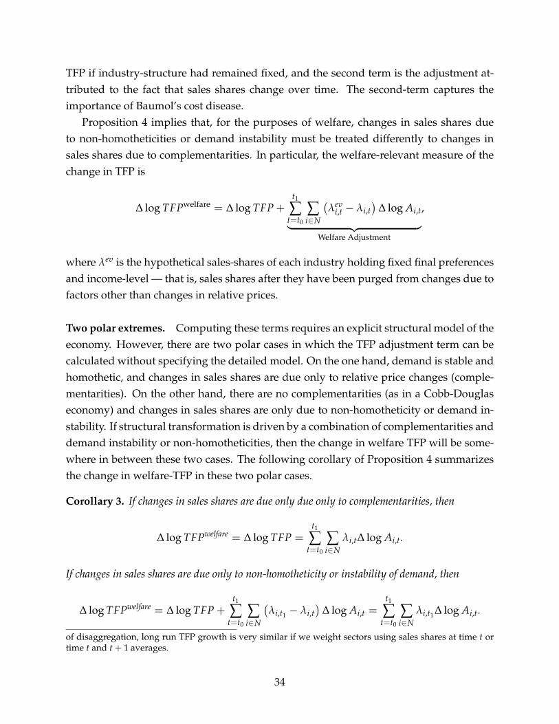
TFP if industry-structure had remained fixed, and the second term is the adjustment at-tributed to the fact that sales shares change over time. The second-term captures theimportance of Baumol’s cost disease.

Proposition 4 implies that, for the purposes of welfare, changes in sales shares dueto non-homotheticities or demand instability must be treated differently to changes insales shares due to complementarities. In particular, the welfare-relevant measure of thechange in TFP is

∆ log TFPwelfare = ∆ log TFP +t1

∑t=t0

∑i∈N

(λev

i,t − λi,t)

∆ log Ai,t︸ ︷︷ ︸Welfare Adjustment

,

where λev is the hypothetical sales-shares of each industry holding fixed final preferencesand income-level — that is, sales shares after they have been purged from changes due tofactors other than changes in relative prices.

Two polar extremes. Computing these terms requires an explicit structural model of theeconomy. However, there are two polar cases in which the TFP adjustment term can becalculated without specifying the detailed model. On the one hand, demand is stable andhomothetic, and changes in sales shares are due only to relative price changes (comple-mentarities). On the other hand, there are no complementarities (as in a Cobb-Douglaseconomy) and changes in sales shares are only due to non-homotheticity or demand in-stability. If structural transformation is driven by a combination of complementarities anddemand instability or non-homotheticities, then the change in welfare TFP will be some-where in between these two cases. The following corollary of Proposition 4 summarizesthe change in welfare-TFP in these two polar cases.

Corollary 3. If changes in sales shares are due only due only to complementarities, then

∆ log TFPwelfare = ∆ log TFP =t1

∑t=t0

∑i∈N

λi,t∆ log Ai,t.

If changes in sales shares are due only to non-homotheticity or instability of demand, then

∆ log TFPwelfare = ∆ log TFP +t1

∑t=t0

∑i∈N

(λi,t1 − λi,t

)∆ log Ai,t =

t1

∑t=t0

∑i∈N

λi,t1∆ log Ai,t.

of disaggregation, long run TFP growth is very similar if we weight sectors using sales shares at time t ortime t and t + 1 averages.

34

In the first case, since preferences are homothetic and stable, welfare-TFP is equal toTFP in the data. In the second case, since there are no complementarities in productionor demand, sales shares do not respond to productivity changes. In order to hold utilityand preferences fixed at their final value, we must compute welfare-TFP using terminalsales shares.

To quantify Corollary 3, we use US-KLEMS data on sales shares and TFP growth for61 private-sector industries. We calculate changes in industry-level gross-output TFP fol-lowing the methodology of Jorgenson et al. (2005) and Carvalho and Gabaix (2013). Theconstant-initial-sales-share term grows by around 58 log points (or 78%), whereas thechain-linked change in aggregate TFP grew by around 47 log points (or 60%). Hence,Baumol’s cost-disease caused aggregate TFP to fall by−10 log points, reducing aggregateproductivity growth by around 23 percent (from 78% to 60%). Using Corollary 3, if weassume that structural transformation is due solely to non-homotheticities or demand in-stability, then the growth in welfare-relevant TFP from 1948-2014 has been 37 log points(or 46%) instead of the measured 47 log points (or 60%) — that is, to say, a 23 percent ad-ditional reduction in the growth rate. In other words, the adjustment necessary to correctfor demand-driven structural transformation is roughly twice as big (in log terms) as theone necessary to account for complementarities related to relative prices.

To understand why the necessary adjustment is roughly twice as big, consider thesecond-order approximation in Proposition 4. Up to a second-order approximation, wecan write

∆ log TFPwelfare ≈ ∆ log TFP +12

[∑i∈N

∂λi

∂ log x∆ log x +

∂λi

∂ log v∆ log v

]∆ log Ai, (21)

where

∆ log TFP ≈ ∑i∈N

λi,t0∆ log Ai +12 ∑

i∈N∆λi∆ log Ai.

If changes in sales shares are due entirely to demand-driven factors, then the term insquare brackets in (21) is equal to ∑i∈N ∆λi∆ log Ai, so

∆ log TFPwelfare ≈ ∑i∈N

λi,t0∆ log Ai + ∑i∈N

∆λi∆ log Ai.

In other words, the adjustment to the initial sales shares must be roughly twice as largeas the adjustment to the initial sales shares caused by complementarities. These second-

35

order approximations are more accurate if changes in sales shares are well-approximatedby linear time trends, and the surprising accuracy of the second-order approximation is aresult of this fact.

The reasoning above implies that the welfare adjustment to bring measured TFP inline with welfare may be as high as 23 percent. However, it may also be as small as zero,if the data can be perfectly explained using only complementarities.

Quantitative illustration away from two polar extremes. In practice, both complemen-tarities and non-homotheticities are likely to play an important role in explaining struc-tural transformation. To dig deeper into the size of the welfare adjustment, we use asimplified version of the model introduced in Section 4 calibrated to the US economy, ac-counting for input-output linkages and complementarities, and use the model to quantifythe size of the welfare-adjustment as a function of the elasticities of substitution.

Remarkably, Proposition 4 implies that to compute the welfare-relevant change in TFP,we must only supply the information necessary to compute λev — that is, we do not needto model the non-homotheticities or demand-shocks themselves, and the exercise requiresno information on the functional form of non-homotheticities or the slope of Engel curvesor magnitude of income elasticities conditional on knowing the elasticities of substitution.

We map the model to the data as follows. We assume that the constant-utility final de-mand aggregator has a nested-CES form. There is an elasticity θ0 across the three groupsof industries: primary, manufacturing, and service industries. The inner nest has elastic-ity of substitution θ1 across industries within primary (2 industries), manufacturing (24industries), and services (35 industries).34 Production functions are also assumed to havenested-CES forms: there is an elasticity of substitution θ2 between the bundle of inter-mediates and value-added, and an elasticity of substitution θ3 across different types ofintermediate inputs. For simplicity, we assume there is only one primary factor of pro-duction (a composite of capital and labor). We solve the non-linear model by repeatedapplication of Proposition 7.35

We calibrate the CES share parameters so that the model matches the 2015 input-output tables provided by the BEA. For different values of the elasticities of substitution

34In order to map this nested structure to our baseline model, good 0 is a composite of good 1-3, wheregood 1 is a composite of primary industries, good 2 is a composite of manufacturing industries, and good3 is a composite of service industries. Goods 4-65 are the disaggregated industries. Finally, good 66 is thesingle factor of production.

35We calculate TFP shocks by industry in the data allowing for cross-industry variation in capital andlabor shares, and then feed these shocks as a primitive into our one-factor model (alternatively, in order toallow for industry variation in capital intensity while keeping the one-factor simplicity, we must assumethat labor and capital are perfect substitutes).

36

(θ0, θ1, θ2, θ3) we feed changes in industry-level TFP (going backwards, from 2015 to 1960)into the model and compute the resulting change in aggregate TFP. This number repre-sents the welfare-relevant change in aggregate TFP. We report the results in Table 1.

Table 1: The percentage change in measured and welfare-relevant TFP in the US from1948 to 2014.

(θ0, θ1, θ2, θ3) (1,1,1,1) (0.5,1,1,1) (1,0.5,1,1) (1,1,0.5,1) (1,1,1,0.5)

Welfare TFP 46% 46% 54% 48% 55%Measured TFP 60% 60% 60% 60% 60%

The first column in Table 1 shows the change in welfare-relevant TFP assuming thatthere are no complementarities (all production and consumption functions are Cobb-Douglas). In this case, all changes in sales shares in the data are driven by non-homotheticitiesor demand-instability, and hence welfare-relevant TFP has grown more slowly than mea-sured TFP, exactly as discussed in the previous section. The other columns show how theresults change given lower elasticities of substitution. As we increase the strength of com-plementarities, we reduce the size of changes in sales shares due to non-homotheticitiesor demand-instability, which in turn reduces the gap between measured and welfare-relevant productivity growth.

Table 1 also shows that not all elasticities of substitution are equally important. Theresults are much more sensitive to changes in the elasticity of substitution across more dis-aggregated categories, like materials, than aggregated categories, like agriculture, manu-facturing, and services. In Appendix H, we show that this is an intuitive consequence ofProposition 6.

5.2 Aggregation Bias with Firm-Level Shocks

In the previous application, we considered a long-run industry-level application. Sinceindustry-level sales shares are relatively stable over short-horizons, given industry-leveldata, biases in real GDP and consumption are likely to be modest at high frequency. How-ever, this does not mean that these biases are necessarily absent from short-run data.

Whereas industry sales shares are stable at high frequency, firm or product-level salesshares are highly volatile even over the very short-run. If firms’ or products’ supply anddemand shocks are correlated, then measured industry-level output is biased relativeto what is relevant for welfare, even if all firms are infinitesimal within their industry.Furthermore, these biases in industry-level data are not diversified away as we aggregate,even if all industries are infinitesimal in the aggregate economy. If these firm-level supply

37

and demand shocks are persistent, then this bias becomes even larger as we lengthen thehorizon. Finally, if we start with industry-level (rather than firm-level) data, we are rulingout the existence of these biases by construction.

To make these points formally, we rely on a specification of our model with an explicitindustrial structure.

Definition 6 (Industrial Structure). An economy has an industry structure if the followingconditions hold:

i. Each firm i belongs to one, and only one, industry I. Firms in the same industryshare the same constant-returns-to-scale production function up to a firm-specificHicks-neutral productivity shifter Ai.

ii. The representative household has homothetic preferences over industry-level goods,where the Ith industry-level consumption aggregator is

cI =

(∑i∈I

biI xicζ I−1

ζ Ii

) ζ Iζ I−1

,

where ci are consumption goods purchased by the household from firm i in industryI and xi are firm-level demand shocks.

iii. Inputs purchased by any firm j from firms i in industry I are aggregated accordingto

mjI =

(∑i∈I

siImσI−1

σIji

) σIσI−1

,

where mji are inputs purchased by firm j from firm i, and siI is a constant.

Input-output and production network models that are disciplined by industry-leveldata typically have an industry structure of the form defined above. For such economies,we can characterize the bias in real GDP relative to welfare easily.

Proposition 8 (Aggregation Bias). For models with an industry structure, in response to firm-level supply shocks ∆ log A and demand shocks ∆ log x, we have

∆ log EVM ≈ ∆ log Y +12 ∑

i∈IbICovb(I)

(∆ log x(i), ∆ log A(i)) + Θ,

where bI is industry I’s share of final demand and b(I) is a vector whose ith element is bi/bI if ibelongs to industry I and zero otherwise. The scalar Θ is the gap between real GDP and welfare

38

in a version of the model with only industry-level shocks.36

In words, Proposition 8 implies that if firms’ productivity and demand shocks arecorrelated with each other (but not necessarily across firms), then there is a gap betweenreal GDP and welfare that does not appear in an industry-level specification of the model.Furthermore, this bias is, to a second-order, additive. That is, the overall bias is the sum ofthe industry-level bias (that we studied in the previous section) plus the additional biasdriven by within-industry covariance of supply and demand shocks.

Identifying supply and demand shocks at the firm-level is notoriously difficult, andmany papers impose that these shocks must be orthogonal in order to estimate them (orto estimate demand elasticities). However, a correlation between firm-level supply anddemand shocks is a natural prediction in models with endogenous customer acquisition(Arkolakis, 2016; Foster et al., 2016; Fitzgerald et al.; 2016), as we discuss in Section 6.A detailed quantitative investigation of this issue is beyond the scope of this paper, butProposition 8 can be used for a back-of-the-envelope calculation.

As a numerical illustration, suppose that firm- or product-level demand shocks andTFP shocks at annual frequency have a standard deviation of 0.5 and 0.2 log points, andsuppose that they have a correlation of 0.2. Proposition 8 implies that, up to a second-order approximation and at annual frequency, the gap between welfare-relevant industryoutput and measured industry output is around 1

2 × 0.2 × 0.5 × 0.2 = 1%.37 If theseindustry-level covariances are the same across all industries, then the gap between realGDP and welfare induced by firm-level shocks is also 1% at annual frequency. This isa one-off steady-state adjustment that does not compound over time (every year, thechange in welfare would be 1% higher than real GDP) if the shocks are independent overtime.

To continue this thought experiment, note that if supply and demand shocks at thefirm level are persistent, then the bias grows over time. For example, suppose that firm-level supply and demand shocks are both AR(1) processes with persistence parameters

36More specifically,

Θ =12 ∑

i∈I∑j∈J

[EbI (∆ log AiI)

(∂bI

∂ log xj

)+ EsI (∆ log AiI)

(∂λ

fI

∂ log xj

)]∆ log xj,

where λfI = λI − bI is the sales share of industry I excluding sales to the household. In words, Θ is

proportional to the product of changes in industry-level sales shares caused by demand shocks times theindustry-level (sales-weighted) productivity shocks.

37The gap would be around 2% based on statistics for TFPQ and demand shocks reported in Table 2 ofEslava and Haltiwanger (2021) using Colombian data. We obtain very similar numbers if we compute thegap exactly (numerically) or if we use the second-order approximation in Proposition 8

39

ρA ∈ [0, 1] and ρx ∈ [0, 1]. Then the gap between welfare and real GDP in period Trelative to some period 0 due to firm-level shocks is (suppressing industry sub-indices)

Covb(∆ log xT, ∆ log AT) =1− (ρxρA)

T

1− (ρxρA)Covb(∆ log x1, ∆ log A1).

Hence, as we expand the horizon, the gap between real GDP and welfare becomes larger.In the limit where supply and demand shocks are correlated random walks, the gap ex-pands without bound as we lengthen the horizon. If the persistence parameters are bothequal to 0.9, then the asymptotic gap between welfare and real GDP is around 5 timeslarger than the one-period gap.

5.3 Path Dependence of Real GDP with an Application to Covid-19

In our last application, we switch from focusing on welfare to considering the propertiesof real GDP in the presence of unstable or non-homothetic preferences. We apply ouranalysis to one specific and noteworthy instance of demand instability: the onset of theCovid-19 crisis. As shown by Corollary 1 changes in real consumption measure changesin welfare accurately if, and only if, preferences are stable and homothetic. The questionthat begs to be asked is: does the change in real GDP or real consumption measure the change inany stable function of allocations when preferences are unstable or non-homothetic? The gradienttheorem for line integrals provides an answer. If sales shares are not derivatives of somestable scalar-valued function, then the change in real GDP between two allocations canbe any arbitrary number depending on the path taken (see Hulten, 1973).

This means that whenever preferences are non-homothetic or unstable, changes in realconsumption (or real GDP) generically depend on the path and timing of shocks, unlikechanges in welfare, which depend only on the initial and final allocation.38 To see this,suppose final demand is homothetic but unstable, and the economy faces supply shocks∆ log A and demand shocks ∆ log x. Consider two different paths for how the shocksunfold: under path SD the supply shocks arrive first and then the demand shocks, andunder DS the demand shocks arrive first and then the supply shocks. A corollary ofProposition 5 is then the following.

Corollary 4 (Path Dependence and Timing of Shocks). If preferences are homothetic, then

∆ log YSD = EVM(At0 , At1 ; xt0), and ∆ log YDS = EVM(At0 , At1 ; xt1),38If real consumption is calculated using fixed weights over time rather than as a Divisia index, then

changes in real consumption are not path dependent, but differ from welfare changes (even if preferencesare stable and homothetic).

40

where ∆ log YSD and ∆ log YDS denote real GDP computed under SD and DS, respectively.

That is, the change in real GDP under the first path measures something different thanthe change in real GDP under the second path. In general, the increase in real GDP islarger if price falls (or productivity rises) later for goods that are subject to earlier positivedemand shocks.39 If we go from the initial allocation to the final one along the path SDand then come back along DS, real GDP will be different even though we are back atthe exact same allocation. Hence, how fast the economy recovers from a shock like theCovid-19 crisis can be affected by irrelevant details like the order in which supply anddemand conditions revert to normal.

Disconcerting as this path dependence problem of real GDP (and other Divisia indices)may be, it is tempting to dismiss it as a theoretical curiosity. However, far from being anexotic theoretical possibility, path-dependence is a well-known problem for practitionerswhen dealing with high-frequency data. Most manuals on index number construction,for example OECD et al. (2004), warn against using chain-weighted indices for high fre-quency data.

The term “chain drift” bias in national accounting describes a situation when a chainedindex measures an overall change between t0 and t1 even though all prices and quantitiesin t0 and t1 are identical. The gradient theorem for line integrals implies that this musthappen if the weights are not derivatives of a stable potential function, even if prices andquantities of all goods are well-measured over time.

Chain drift bias appears when movements in prices and quantities are oscillatory,where changes that take place over some periods are reversed in subsequent periods.This happens frequently at sub-annual frequencies, so the usual advice given to practi-tioners is to avoid these problems by not chaining their data too frequently. Intuitively, ifwe only chain indices at annual or lower frequencies, then it will very rarely be the casethat prices and quantities will revert back to their previous values, and hence, we will notobserve changes in the aggregate even though every price and quantity has returned toan initial value.

Chaining at low frequency does not solve the problem however, it simply avoids hav-ing to confront it by ensuring that prices and quantities never revert back to their previousvalues. But the path dependence problem that causes chain drift does not become less se-vere at lower frequencies, it simply becomes less noticeable. The approach we advocate inthis paper, which corrects the index for instability and non-homotheticity, has the virtueof restoring path independence.

39This implies that, in the presence of demand instability, the order of reforms that increase sectoralproductivity matters for the magnitude of the overall increase in real GDP

41

The Covid-19 recession provides an illustrative case in point. During the first twoquarters of 2020, employment and production rapidly contracted in most economies aroundthe world. This contraction was unusual in that it fell very unevenly across different in-dustries. The sales shares of some sectors, like air transportation or entertainment venues,collapsed while those of other sectors, like retail trade, rose. These changes are difficult tojustify on the basis of observed price changes since relative price movements across sec-tors were relatively modest. Given the fact that producing and consuming some goodsrequires much more face-to-face contact than others, it is natural to suppose that non-price factors likely played an important role in the observed changes in sales shares.40

That is, final demand across sectors as a function of measured prices was unstable duringthis period.

We now consider how sensitive the change in real GDP can be to the exact timing ofthe supply and demand shocks. To answer this question, we use a modified version ofthe structural model introduced above. Since we are interested in a short-run application,we assume that factor markets are segmented by industry, so that labor and capital ineach industry is inelastically supplied. We then calibrate share parameters to match theinput-output table in 2018, and consider a range of elasticities of substitution. Follow-ing Baqaee and Farhi (2020), we hit the economy with a vector of primitive supply anddemand shocks.41 The supply shocks are reductions in factor endowments, calibrated tomatch peak-to-trough reductions in hours worked by sector from January, 2020 to May,2020. The primitive demand shocks are shifters in final demand, calibrated to matchthe observed peak-to-trough reductions in personal consumption expenditures by sectorfrom January, 2020 to May, 2020 (given the supply shocks). The details of this calibrationexercise can be found in Appendix D.

Table 2 reports the results. We consider three different calibrations informed by em-pirical estimates from Atalay (2017) and Boehm et al. (2015): high complementarities,medium complementarities, and no complementarities (Cobb-Douglas). The high com-

40These non-price factors could be changes in quality, changes in preferences, or changes in governmentpolicies during the pandemic. For our purposes in this application (i.e. path dependence of real GDPas measured in the data), it does not matter what is the source of demand instability at measured prices.Of course, in order to assess the welfare costs of Covid-19, the source of demand instability is important.However, since consumers do not make choices about whether or not they live in a world with Covid-19, the welfare costs of Covid-19 are not revealed by their choices. For example, choices between goingto restaurants or cooking at home reveal preferences between these two goods conditional on living in aworld with a pandemic. What is not revealed by these choices are preferences over restaurants with andwithout pandemics, and cooking at home with and without pandemics. For this reason, we refrain fromanalyzing the welfare costs of Covid-19 in this application.

41For related analysis of Covid-19 induced supply shocks, see e.g. Bonadio et al. (2020) and Barrot et al.(2020). For related analysis of Covid-19 induced demand shocks, see Cakmakli et al. (2020).

42

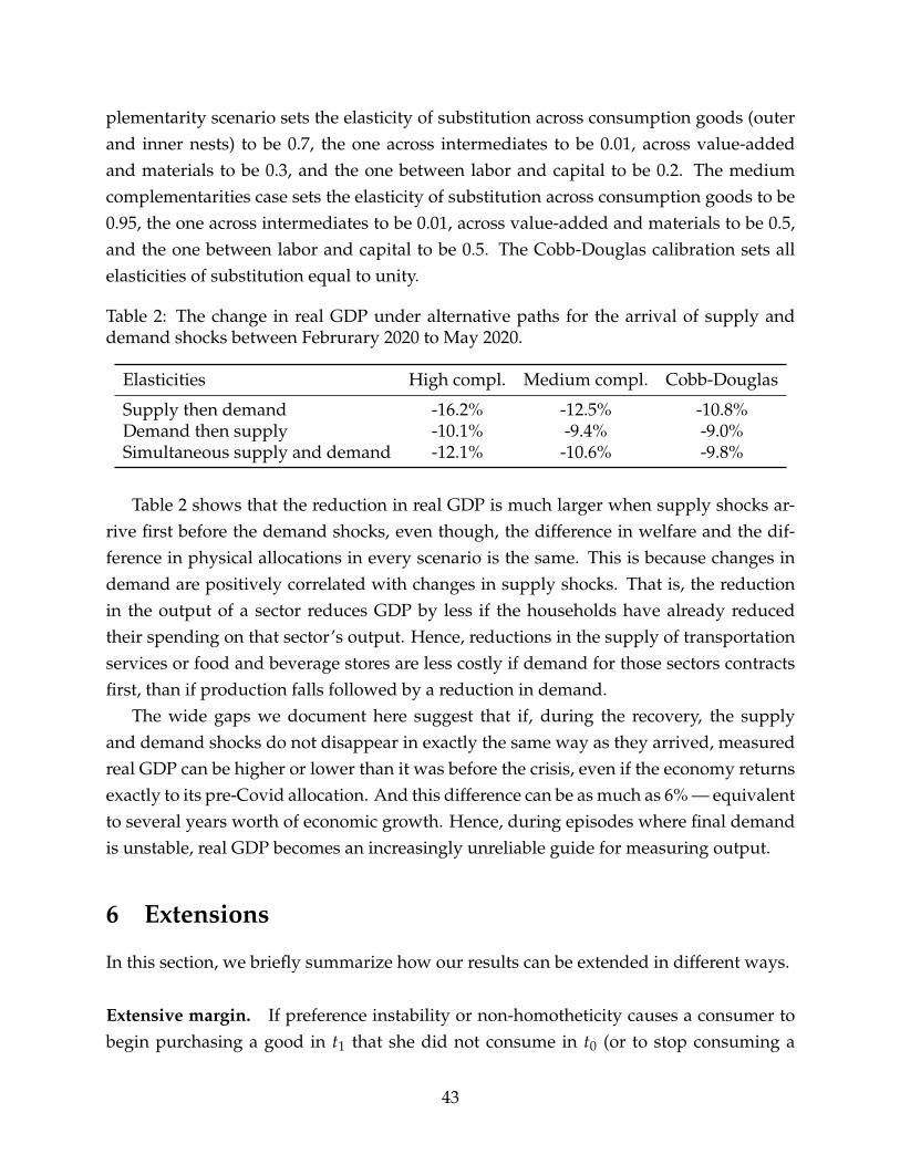
plementarity scenario sets the elasticity of substitution across consumption goods (outerand inner nests) to be 0.7, the one across intermediates to be 0.01, across value-addedand materials to be 0.3, and the one between labor and capital to be 0.2. The mediumcomplementarities case sets the elasticity of substitution across consumption goods to be0.95, the one across intermediates to be 0.01, across value-added and materials to be 0.5,and the one between labor and capital to be 0.5. The Cobb-Douglas calibration sets allelasticities of substitution equal to unity.

Table 2: The change in real GDP under alternative paths for the arrival of supply anddemand shocks between Februrary 2020 to May 2020.

Elasticities High compl. Medium compl. Cobb-Douglas

Supply then demand -16.2% -12.5% -10.8%Demand then supply -10.1% -9.4% -9.0%Simultaneous supply and demand -12.1% -10.6% -9.8%

Table 2 shows that the reduction in real GDP is much larger when supply shocks ar-rive first before the demand shocks, even though, the difference in welfare and the dif-ference in physical allocations in every scenario is the same. This is because changes indemand are positively correlated with changes in supply shocks. That is, the reductionin the output of a sector reduces GDP by less if the households have already reducedtheir spending on that sector’s output. Hence, reductions in the supply of transportationservices or food and beverage stores are less costly if demand for those sectors contractsfirst, than if production falls followed by a reduction in demand.

The wide gaps we document here suggest that if, during the recovery, the supplyand demand shocks do not disappear in exactly the same way as they arrived, measuredreal GDP can be higher or lower than it was before the crisis, even if the economy returnsexactly to its pre-Covid allocation. And this difference can be as much as 6% — equivalentto several years worth of economic growth. Hence, during episodes where final demandis unstable, real GDP becomes an increasingly unreliable guide for measuring output.

6 Extensions

In this section, we briefly summarize how our results can be extended in different ways.

Extensive margin. If preference instability or non-homotheticity causes a consumer tobegin purchasing a good in t1 that she did not consume in t0 (or to stop consuming a

43

good that she was previously consuming), then our global and local formulas apply tothat consumer without change.

To make this more explicit, consider a consumer whose preferences are representedby the utility function (∫ x∗

0c(z)

σ−1σ dz

) σσ−1

, (22)

where goods are indexed by z ∈ [0, 1] but the consumer only values goods z ∈ [0, x∗].In this situation, x∗ is a preference parameter, where goods z ∈ (x∗, 1] are available at afinite price, but the consumer chooses not to consume them.

Consider how the welfare of the consumer changes accounting for the fact that x∗ canchange between t0 and t1. The following is an application of Lemma 1.

Proposition 9 (New Goods Due to Taste Shocks). Consider a household with preferences de-fined by (22). Up to a second-order approximation,

∆ log EVm ≈ ∆ log Y +12

b(x∗)∆x∗ [Eb [∆ log p]− ∆ log p(x∗)] .

In words, the gap between welfare and real GDP depends on product of sales sharesat the cut-off b(x∗), the change in the cut-off ∆x∗, and the difference between inflation atthe cut-off versus average inflation. If new goods are added ∆x∗ > 0, and the new goodsexperienced lower than average inflation, then welfare is higher than what is detected byreal GDP. However, this adjustment is second-order (since it involves products of ∆), andto a first-order, real GDP is equal to the true change in the cost of living.

It is interesting to contrast Proposition 9 to the well-known new-goods adjustmentdue to Feenstra (1994), which, to a first-order approximation, is

∆ log EVm = ∆ log Y +1

1− σ∆ log

[∫C

b(z)dz]

, (23)

where C is the set of continuing goods and the integral is their share in expenditures. Thedifference in these results is due to a difference in interpretation. Under the interpretationin Proposition 9, the change in the extensive margin is caused by a change in tastes —that is, the goods were previously available to the consumer in the initial period but theconsumer chose not to consume them (or goods are available in the final period, but theconsumer chose to stop consuming them). Therefore, when we calculate welfare changes,we simply need to adjust the price index so that it accounts for the price of goods that theconsumer is choosing to consume in the final period. On the other hand, under (23), whenwe compute the change in welfare, we assume that the consumer is unable to consume the

44

new goods in the past or can no longer consume the disappearing goods in the present.That is, under (23), when goods are not consumed they are valued by the consumer butthe implicit price is infinity.

Therefore, if a good is available in t0 and t1, but the consumer does not consume thegood in period t0 and does consume the good in t1 (due to, for example, advertising),an application of (23) is not innocuous. If the change in consumer behavior is due to achange in tastes, as opposed to a change in availability, then no adjustment is necessaryto a first-order, and to a second-order, the relevant adjustment is the one in Proposition 9.

Endogenous separable arguments in the utility function (e.g. leisure). If there aregoods in the utility function that are endogenously chosen but not measured, then anall-encompassing welfare measure must impute shadow prices for these goods (see Jonesand Klenow, 2016). For concreteness, suppose that leisure is the non-measured argumentin the utility function. If leisure is separable from market goods, so that preferences overc are stable when the quantity of leisure changes, then our baseline results apply to themeasured-good component of welfare, even if leisure changes.

Endogenous non-separable arguments in the utility function (e.g. advertising). If theparameters of the utility function x are not separable from goods c, then our welfare ques-tions ask how changes in constraints over c affect welfare holding fixed x. That is, we donot attempt to answer how a change in x itself affects welfare, which may or may not bea question that can be answered. A salient example of x can be advertising, which canchange households ranking over different consumption bundles, and is obviously non-separable from market goods. In principle, advertising may have value to the consumer— that is, the consumer can have preferences over the amount of advertising they wishto be exposed to. If advertising is informative, the consumer’s utility may be increasingin advertising, and equally plausibly, if advertising is manipulative, then utility may bedecreasing in advertising. We do not attempt to answer the question of how much thehousehold values advertising, instead, we hold fixed the amount of advertising42 (or in-deed the weather, chemicals in the brain, and whatever else that affects valuations overconsumption bundles), and measure how changes in the availability of market goods af-fects welfare.

Interestingly, unlike random fluctuations in tastes, advertising is a purposeful eco-nomic activity, and therefore, models of advertising and consumer acquisition, for exam-

42In this sense, our approach is related to Dixit and Norman (1978), who study the welfare implicationsof advertising at either pre- or post-advertising preferences. As argued by Fisher and McGowan (1979), thisdoes not answer the question of what is the value of advertisement taking into account the change in tastes.

45

ple Arkolakis (2016), explicitly predict that changes in tastes induced by advertising willbe correlated with changes in physical productivity, whereby more productive firms willexpend more resources on advertising. This positive correlation means that we shouldexpect real GDP or real consumption measures to be systematically biased in situationswhere advertising plays a large role in consumption choices.

Beyond CES. Our results in Section 4 can be generalized beyond CES functional formsrelatively easily. In Appendix C, we discuss how Proposition 7 must be adjusted to allowfor non-CES production and utility functions.

Heterogeneous agents. Our microeconomic welfare results can be applied in economieswithout representative agents (including open economies). Our macroeconomic welfareresults relied on the assumption that there is a representative agent because, in this case,the competitive equilibrium is maximizing this agent’s welfare.

In economies with heterogeneous agents and non-aggregable preferences, the socialwelfare function (SWF) is not unambiguous. In such economies, every competitive equi-librium maximizes a potentially different SWF (see Negishi, 1960). Whereas to a first-order, changes in real output will coincide with changes in the SWF that is being maxi-mized in the initial competitive equilibrium, at higher orders this relation breaks down.

If one commits to a particular SWF, results like the ones we developed in Section 3 canbe used to correct the gap between social welfare and real GDP. For example, consider thefollowing utilitarian SWF which weights the welfare of each agent i by their initial sharein expenditures,

W = ∑i∈I

piYi

∑j∈I pjYj

[EVm

i¯EVm

i.

]This SWF is maximized in the initial equilibrium. Since the parameters of this SWFchange in response to shocks that redistribute income, it is as if the social planner hasunstable preferences. This instability can create a gap between social welfare and GDPeven if preferences of individual agents are stable and homothetic.

For this case, in Appendix E we show that under the assumptions in Section 3, to asecond-order approximation,

∆ log W = ∆ log Y +12

Covχ (Eb[∆ log p], ∆ log I −Eb[∆ log p]) ,

where χ is the initial distribution of expenditures by each agent, and Eb[∆ log p] is the vec-tor of inflation rates and ∆ log I is the vector of nominal income changes for each house-

46

hold. The change in social welfare is greater than the change in real GDP if changes inreal income covary positively with inflation across households. There is no bias if prefer-ences are aggregable, in which case ∆ log p is uniform across households, if real incomegrowth is uniform or, more generally, if changes in household-level inflation rates areuncorrelated with changes in real income.

7 Conclusion

In this paper, we provide a characterization of the gap, due to substitution bias, betweenstandard measures of consumption and welfare that appear when preferences are non-homothetic or unstable. We characterize this bias in both partial and general equilibrium,and show that it can be large over long horizons relevant for long-run growth, and short-horizons when expenditure shares change rapidly (as in they do with firm or product-level sales shares).

Although our motivation and applications have focused on shocks across time, ourresults can also be applied to compare welfare across locations in space. Variation intastes is likely to be even more significant across space than across time (see, e.g. Deaton,2003 and Argente et al., 2020). Applying our results in a spatial context is an interestingavenue for future work.

ReferencesAcemoglu, D., V. M. Carvalho, A. Ozdaglar, and A. Tahbaz-Salehi (2012). The network origins of aggregate

fluctuations. Econometrica 80(5), 1977–2016.Acemoglu, D. and V. Guerrieri (2008). Capital deepening and nonbalanced economic growth. Journal of

political Economy 116(3), 467–498.Aghion, P., A. Bergeaud, T. Boppart, P. J. Klenow, and H. Li (2019). Missing growth from creative destruc-

tion. American Economic Review 109(8), 2795–2822.Alder, S., T. Boppart, and A. Müller (2019). A theory of structural change that can fit the data.Argente, D. O., C.-T. Hsieh, and M. Lee (2020, September). Measuring the cost of living in mexico and the

us. Working Paper 27806, National Bureau of Economic Research.Arkolakis, C. (2016). A unified theory of firm selection and growth. The Quarterly Journal of Economics 131(1),

89–155.Atalay, E. (2017). How important are sectoral shocks? American Economic Journal: Macroeconomics (Forth-

coming).Atkin, D., B. Faber, T. Fally, and M. Gonzalez-Navarro (2020, March). Measuring Welfare and Inequality

with Incomplete Price Information. NBER Working Papers 26890, National Bureau of Economic Re-search, Inc.

47

Auer, R., A. Burstein, S. Lein, and J. Vogel (2021). Unequal expenditure switching: Evidence from switzer-land.

Balk, B. M. (1989). Changing consumer preferences and the cost-of-living index: theory and nonparametricexpressions. Journal of Economics 50(2), 157–169.

Baqaee, D. and E. Farhi (2019a). Networks, barriers, and trade. Technical report, National Bureau of Eco-nomic Research.

Baqaee, D. and E. Farhi (2020). Supply and demand in disaggregated keynesian economies with an appli-cation to the covid-19 crisis. Technical report, National Bureau of Economic Research.

Baqaee, D. R. and E. Farhi (2019b). Productivity and misallocation in general equilibrium. The QuarterlyJournal of Economics 135(1), 105–163.

Baqaee, D. R. and E. Farhi (2019c). The Macroeconomic Impact of Microeconomic Shocks: Beyond Hulten’sTheorem. Econometrica 87(4), 1155–1203.

Barrot, J.-N., B. Grassi, and J. Sauvagnat (2020). Sectoral effects of social distancing. Available at SSRN.Basu, S., L. Pascali, F. Schiantarelli, and L. Serven (2012). Productivity and the welfare of nations. Technical

report, National Bureau of Economic Research.Baumol, W. J. (1967). Macroeconomics of unbalanced growth: the anatomy of urban crisis. The American

economic review, 415–426.Boehm, C., A. Flaaen, and N. Pandalai-Nayar (2015). Input linkages and the transmission of shocks: Firm-

level evidence from the 2011 tohoku earthquake.Bonadio, B., Z. Huo, A. A. Levchenko, and N. Pandalai-Nayar (2020). Global supply chains in the pandemic.

Technical report.Boppart, T. (2014). Structural change and the kaldor facts in a growth model with relative price effects and

non-gorman preferences. Econometrica 82(6), 2167–2196.Buera, F. J. and J. P. Kaboski (2009, 04-05). Can Traditional Theories of Structural Change Fit The Data?

Journal of the European Economic Association 7(2-3), 469–477.Buera, F. J., J. P. Kaboski, and R. Rogerson (2015). Skill biased structural change. Technical report, National

Bureau of Economic Research.Cakmakli, C., S. Demiralp, S. Kalemli-Ozcan, S. Yesiltas, and M. A. Yildirim (2020, May). Covid-19 and

emerging markets: An epidemiological multi-sector model for a small open economy with an applicationto turkey. Working Paper 27191, National Bureau of Economic Research.

Carvalho, V. and X. Gabaix (2013). The Great Diversification and its undoing. The American EconomicReview 103(5), 1697–1727.

Carvalho, V. M. and A. Tahbaz-Salehi (2018). Production networks: A primer.Caves, D. W., L. R. Christensen, and W. E. Diewert (1982). The economic theory of index numbers and the

measurement of input, output, and productivity. Econometrica: Journal of the Econometric Society, 1393–1414.

Comin, D. A., D. Lashkari, and M. Mestieri (2015). Structural change with long-run income and priceeffects. Technical report, National Bureau of Economic Research.

Deaton, A. (2003). Adjusted indian poverty estimates for 1999-2000. Economic and political Weekly, 322–326.Dixit, A. and V. Norman (1978). Advertising and welfare. The Bell Journal of Economics, 1–17.Domar, E. D. (1961). On the measurement of technological change. The Economic Journal 71(284), 709–729.Eslava, M. and J. C. Haltiwanger (2021). The life-cycle growth of plants: The role of productivity, demand

and wedges. Technical report, National Bureau of Economic Research.

48

Fally, T. (2020). Integrability, generalized separability, and a new class of demand systems.Feenstra, R. C. (1994). New product varieties and the measurement of international prices. The American

Economic Review, 157–177.Fisher, F. M. and J. J. McGowan (1979, Autumn). Advertising and Welfare: Comment. Bell Journal of Eco-

nomics 10(2), 726–727.Fisher, F. M. and K. Shell (1968). Taste and quality change in the pure theory of the true cost of living index.

Chicago: Aldine Publishing.Fitzgerald, D., S. Haller, and Y. Yedid-Levi (2016). How exporters grow. Technical report, National Bureau

of Economic Research.Foster, L., J. Haltiwanger, and C. Syverson (2016). The slow growth of new plants: learning about demand?

Economica 83(329), 91–129.Gabaix, X. (2011). The granular origins of aggregate fluctuations. Econometrica 79(3), 733–772.Hamilton, B. W. (2001, June). Using engel’s law to estimate cpi bias. American Economic Review 91(3), 619–

630.Hausman, J. A. (1996). Valuation of new goods under perfect and imperfect competition. In The economics

of new goods, pp. 207–248. University of Chicago Press.Herrendorf, B., R. Rogerson, and A. Valentinyi (2013). Two perspectives on preferences and structural

transformation. American Economic Review 103(7), 2752–89.Hicks, J. R. (1940). The valuation of the social income. Economica 7(26), 105–124.Hulten, C. R. (1973). Divisia index numbers. Econometrica: Journal of the Econometric Society, 1017–1025.Hulten, C. R. (1978). Growth accounting with intermediate inputs. The Review of Economic Studies, 511–518.Jones, C. I. and P. J. Klenow (2016). Beyond gdp? welfare across countries and time. American Economic

Review 106(9), 2426–57.Jorgenson, D. W., M. S. Ho, K. J. Stiroh, et al. (2005). productivity, volume 3: information technology and

the american growth resurgence. MIT Press Books 3.Kongsamut, P., S. Rebelo, and D. Xie (2001). Beyond Balanced Growth. Review of Economic Studies 68(4),

869–882.Negishi, T. (1960). Welfare economics and existence of an equilibrium for a competitive economy. Metroe-

conomica 12(2-3), 92–97.Ngai, L. R. and C. A. Pissarides (2007). Structural change in a multisector model of growth. American

economic review 97(1), 429–443.Nordhaus, W. D. et al. (2008). Baumol’s diseases: A macroeconomic perspective. The BE Journal of Macroe-

conomics 8(1), 1–39.OECD, T. W. Bank, T. U. N. E. C. for Europe, S. O. of the European Communities, and Luxembourg (2004).

Consumer price index manual: Theory and practice. International Monetary Fund.Redding, S. J. and D. E. Weinstein (2020). Measuring aggregate price indices with taste shocks: Theory and

evidence for ces preferences. The Quarterly Journal of Economics 135(1), 503–560.Samuelson, P. A. and S. Swamy (1974). Invariant economic index numbers and canonical duality: survey

and synthesis. The American Economic Review 64(4), 566–593.Syverson, C. (2017). Challenges to mismeasurement explanations for the us productivity slowdown. Journal

of Economic Perspectives 31(2), 165–86.

49

[Appendix To Be Added]

50

Appendix A Proofs

Proof of Lemma 1. By definition,

EVm = loge (pt0 , v(pt1 , It1 ; xt1); xt1)

e (pt0 , v(pt0 , It0 ; xt1); xt1)

= loge (pt0 , v(pt1 , It1 ; xt1); xt1)

e (pt0 , v(pt0 , It0 ; xt1); xt1)

e (pt1 , v(pt1 , It1 ; xt1); xt1)

e (pt1 , v(pt1 , It1 ; xt1); xt1)

= loge (pt0 , v(pt1 , It1 ; xt1); xt1)

It0

It1

e (pt1 , v(pt1 , It1 ; xt1); xt1).

To finish, rewrite

loge (pt0 , v(pt1 , It1 ; xt1); xt1)

e (pt1 , v(pt1 , It1 ; xt1); xt1)= −

∫ t1

t0

∂ log e(p, v(pt1 , It1 ; xt1); xt1)

∂ log pd log p

dtdt,

and use the Shephard’s lemma to express the price elasticity of the expenditure functionin terms of budget shares.

Proof of Proposition 1. Combine Lemma 1 with the definition of real consumption.

Proof of Corollary 1. From Proposition 1, given any change in prices, income, and prefer-ences, EVm − ∆ log Y = 0 if, and only if, b = bev, which is the case if, and only if, budgetshares do not depend on the level of utility and x – that is preferences are homothetic andstable.

Proof of Lemma 2. Differentiate real consumption

∆ log Y =∫ t1

t0

d log I(t)−∑i

bi(p(t), u(t); x(t))d log pi

dtdt

twice with respect to t1 and evaluate the derivative at t1 = t0. This yields the desiredexpression.

Proof of Proposition 2. By Lemma 1:

EV = ∆ log I −∫ t1

t0∑

i

∂ log e(p, v(pt1 , xt1), xt1)

∂ log pd log pd log t

d log t

51

Differentiate EV twice with respect to t1 and evaluate the derivative at t1 = t0.

dEVdt1

=d log I

dt−∑

i

∂ log e(p, v(pt1 , xt1), xt1)

∂ log pi

d log pi

d log t−

−∫ t1

t0∑

id log v

∂2 log e(p, v(pt1 , xt1), xt1)

∂ log u∂ log pid log pi

−∫ t1

t0∑

id log x

∂2 log e(p, v(pt1 , xt1), xt1)

∂ log x∂ log pid log pi

d2EVdt2

1= −∑

ibi

d2 log pd log t2 −∑

i∑

j

∂2 log e(p, v(pt1 , xt1), xt1)

∂ log pi∂ log pjd log pid log pj

− 2 ∑i

d log v∂2 log e(p, v(pt1 , xt1), xt1)

∂ log pi∂ log ud log pi − 2 ∑

id log x′

∂ log e(p, v(pt1 , xt1), xt1)

∂ log pi∂ log xd log pi

= −∑i

∑j

∂bi

∂ log pid log pid log pj −∑

ibi

d2 log pd log t2

− 2 ∑i

d log v∂bi

∂ log ud log pi − 2 ∑

id log x′

∂bi

∂ log xd log pi

= −∑i

[∑

j

∂bi

∂ log pjd log pj + d log v

∂bi

∂ log u+ d log x′

∂bi

∂ log x

]d log pi −∑

ibi

d2 log pd log t2

−∑i

d log v∂bi

∂ log ud log pi −∑

id log x′

∂bi

∂ log xd log pi

= −∑i

dbid log pi −∑i

bid2 log pd log t2 −∑

id log v

∂bi

∂ log ud log pi −∑

id log x′

∂bi

∂ log xd log pi

By Lemma 2, the first two terms are equal to the second-order expansion of ∆ log Y, andthe remaining terms are the bias.

Proof of Proposition 3. By Lemma 2, we have

∆ log Y ≈ ∆ log I −∑i

bi∆ log pi −12 ∑

i∆bi∆ log pi.

Substitute (9) in place of ∆b to get the desired expression. For the bias, note that Proposi-tion 1 implies that

EV − ∆ log Y ≈ −12 ∑

i

[∆bi −∑

j

∂bHi

∂ log pj∆ log pj

]∆ log pi

where bH is the Hicksian budget share (holding fixed utility and demand shifters). Using

52

(9) in place of ∆b above yields the following

∆ log EV − ∆ log Y ≈ −12 ∑

i

[(εi − 1)bi

(d log I −∑

jbj∆ log pj

)+ bi∆ log xi

]∆ log pi,

which can be rearranged to give the desired expression.

Proof of Lemma 3. Setting nominal GDP to be the numeraire, we can write

∆ log Y = −∫ t1

t0

b′d log p

= −∫ t1

t0

b′[−Ψd log A + ΨFd log Λ

]=∫ t1

t0

b′Ψd log A−∫ t1

t0

b′ΨFd log Λ

=∫ t1

t0

λ′d log A−∫ t1

t0

Λd log Λ

=∫ t1

t0

λ′d log A

where the second line uses Proposition 7, and we use the fact that Using λ′ = b′Ψ ,Λ′ = b′ΨF, and b′ΨFd log Λ = Λ′d log Λ = 0 because the factor shares always sum to one:

∑i Λi = 1.

Proof of Proposition 4. We consider the case when preferences are homothetic and unstablefirst, followed by non-homothetic and stable.

Case 1. Since preferences are homothetic, fixing preferences at xt1 , changes in real GDPin the fictional economy are equal to changes in welfare. Changes in real GDP, in thefictional economy, can be expressed in terms of the necessary integral using Lemma 3.

Case 2. Now consider the case with stable but non-homothetic preferences. We suppressdependence on x throughout since it does not change. Without loss of generality, weassume that income is unchanged (since equilibrium prices are only determined relativeto income). As indicated by Proposition 7, changes in equilibrium prices given shocks totechnologies and preferences are given by

d log p = −Ψd log A + ΨFd log Λ. (24)

53

Define a hypothetical economy with fictional households that have stable homotheticpreferences defined by the expenditure function e∗ (p, u) = e (p, v∗) u

v∗ , where v∗ = v(A+

∆A). Budget shares of this fictional consumer are bevi (p) ≡ ∂e(p,v∗)

∂pi. Given any technol-

ogy vector and these preferences, we denote the Leontief inverse matrix by Ψev, budgetshares by bev, and sales shares by λev. Changes in prices satisfy equation (24) under thealternative input-output matrix. We denote by p + ∆pev the equilibrium prices in thishypothetical economy given technologies A + ∆A. Note that p + ∆pev is generically notequal to p + ∆p if preferences in the baseline economy are non-homothetic.

Adding and substracting log e (p + ∆pev, v(A + ∆A)) to the definition of EVM,

EVM = log e (p, v(A + ∆A))− log e (p + ∆pev, v(A + ∆A))

+ log e (p + ∆pev, v(A + ∆A))− log e (p, v(A)) .

By the constant income normalization, the second line is equal to zero. Therefore,

EVM = log e (p, v∗)− log e (p + ∆pev, v∗)

= −∫ t1

t0∑

i

∂ log e(p, v∗)∂ log pi

d log pevi = −

∫ t1

t0∑

ibev

i d log pevi

where d log pevi denotes prices changes in the hypothetical economy as technologies shift

from A to A + ∆A. Following the same steps as in Lemma 3, we obtain

EVM =∫ t1

t0∑

iλev

i d log Ai.

As mentioned earlier, in general, macro and micro welfare changes are not the samewhen preferences are unstable. However, when the PPF is linear, the two coincide.

Proposition 10 (Macro vs. Micro Welfare). When preferences are unstable, macro and microwelfare changes are equal (EVm = EVM) if factor income shares are constant (as in a one factoreconomy).

Proof of Proposition 10. If preferences are stable, the result is immediate by inspecting thewelfare expressions in Propositions 5 and 2 for the case of stable preferences (note thatthe change in real GDP is the same in the micro and macro problems). Consider now aneconomy with unstable preferences. If factor income shares, Λ, are constant, then changesin prices are

d log p = −Ψd log A.

54

sod log x′

∂b∂ log x

d log p = −d log x′∂λ

∂ log xΨd log A

where we used the identity λ′ = b′Ψ. The result is immediate by inspecting the welfareexpressions in Propositions 5 and 2 for the case of unstable preferences.

Proof of Lemma 4. Differentiate real consumption

∆ log Y =∫ t1

t0∑

iλi(A(t); x(t))

d log Ai

dtdt

twice with respect to t1 and evaluate the derivative at t1 = t0. This yields the desiredexpression.

Proof of Proposition 6. Normalize nominal GDP to one. Then, applying Proposition 7 to aone-factor model yields

d log p = −Ψd log A,

so that relative prices do not respond to changes in demand or income. Following Propo-sition 10, EVM = EVm. The result follows from combining Proposition 2 with our expres-sion for d log p and Proposition 7.

Proof of Proposition 7. We normalize nominal GDP to be the numeraire. Then Shephard’slemma implies that, for each i ∈ N

d log pi = −d log Ai + ∑j

Ωijd log pj.

Furthermore, for i ∈ Fd log wi = −d log Ai + d log Λi.

Combining these yields the desired expression for changes in prices

d log p = −Ψd log A + ΨFd log Λ.

To get changes in sales shares, note that

λ = b′Ψ

dλ = d(b′Ψ)

= b′ΨdΩΨ + db′Ψ

55

Ωijd log Ωij = (1− θi)Ωij(d log pj −∑k

Ωikd log pk)

dΩij = (1− θi)CovΩ(i)(d log p, I(j))

∑j

dΩijΨjk = (1− θi)CovΩ(i)(d log p, I(j))Ψjk

= (1− θi)∑j

CovΩ(i)(d log p, Ψjk I(j))

[dΩΨ]ik = (1− θi)CovΩ(i)(d log p, Ψ(k))

Meanwhile

d log bi = (1− θ0)

(d log pi −

(∑

ibid log pi

))+ (εi − 1)d log Y + d log xi

= (1− θ0)CovΩ(0)

(d log p, I(i)

)+ CovΩ(0)

(ε, I(i)

)d log Y + CovΩ(0)

(d log x, I(i)

)∑

idbiΨik = CovΩ(0)

((1− θ0)d log p + εd log Y + d log x, Ψ(k)

)Hence,

dλ′ = λ′dΩΨ + db′Ψ

dλk = ∑i

λi(1− θi)CovΩ(i)(d log p, Ψ(k)) + CovΩ(0)

(ε, Ψ(k)

)d log Y + CovΩ(0)

(d log x, Ψ(k)

)Hence

dλk = ∑i

λi(1− θi)CovΩ(i)(d log p, Ψ(k)) + CovΩ(0)

(ε, Ψ(k)

)d log Y + CovΩ(0)

(d log x, Ψ(k)

).

Proof of Proposition 8. Start by setting nominal GDP to be the numeraire. To model theindustry-structure, for each industry I, add two new CES aggregators. One buys thegood for the household and one buys the good for firms. Let the price of the householdaggregator be given by pc

I and the price of the non-household aggregator be p fI and let

pI be the price of the original industry. Let firm i′s share of industry I from household

56

expenditures be biI . Let the expenditure share of other firms on firm i be siI . We have

∑i∈I

biI = 1

∑i∈I

siI = 1.

Let λcI and λ

fI be sales of industry I to households and firms. Then we have

dλI = dλcI + dλ

fI .

The sales of an individual firm i in industry I is given by

λi = biIλcI + siIλ

fI

dλi = dbiIλcI + biIdλc

I + dsiIλfI + siIdλ

fI

dbiI = CovbI (d log x(iI) + (1− σI)d log A(iI), I(i))

dsiI = CovbI ((1− σI)d log A(iI), I(i)).

The bias in GDP is given by

12

d log x∂λ

∂ log xd log A =

12 ∑

i

[∑

jd log xj

∂λi

∂ log xj

]d log Ai.

Which we can write as

∑i

[∑

jd log xj

∂λi

∂ log xj

]d log Ai = ∑

i

[d log x

∂biI

∂ log xλc

Id log Ai + biId log x∂λc

I∂ log x

d log Ai

+d log x∂siI

∂ log xλ

fI d log Ai + siId log x

∂λfI

∂ log xd log Ai

].

The individual terms of this expression are:

∑i

[d log x

∂biI

∂ log xλc

Id log Ai

]= ∑

iCovbI (d log x(iI), I(i))λ

cId log Ai

= CovbI (d log x(iI), ∑i

I(i)d log Ai)λcI

= CovbI (d log x(iI), d log AiI)λcI ;

57

∑i

[biId log x

∂λcI

∂ log xd log Ai

]= EbI (d log AiI) d log x

∂λcI

∂ log x;

∑i

d log x∂siI

∂ log xλ

fI d log Ai = 0;

and

∑i

siId log x∂λ

fI

∂ log xd log Ai = EsI (d log AiI) d log x

∂λfI

∂ log x.

Of the four terms, two of them depend on changes on industry-level sales shares, oneof them is zero, and the remaining one is the within-industry covariance of supply anddemand shocks in the proposition.

Proof of Proposition 9. Consider a household with preferences given by

C =

(∫ x∗

0c(x)

σ−1σ dx

) σσ−1

.

Note that

λev(x, t, t1) =p(x, t)1−σ(∫ x∗(t1)

0 p(x, t)1−σdx)

λ(x, t) =p(x, t)1−σ(∫ x∗(t)

0 p(x)1−σdx)

HenceEV =

I(∫ x∗(t1)0 p(x)1−σdx

) 11−σ

.

Next

∆ log EV = ∆ log I −∫ t1

t0

∫ x∗(t1)

0λev(x, t, t1)

d log p(x, t)dt

dxdt.

Without loss of generality, let’s normalize changes in nominal income to zero. Let ∂iλev

refer to the partial derivative of λev with respect to its ith argument. Differentiating and

58

evaluating at the initial point, we get

d log EVdt1

= −∫ t1

t0

∫ x∗(t1)

0∂3λev(x, t, t1)

d log p(x, t)dt

dxdt

−∫ t1

t0

λev(x∗(t1), t, t1)d log p(x∗(t1), t)

dtdx∗

dt1dt−

∫ x∗(t1)

0λev(x, t1, t1)

d log p(x, t1)

dt1dx

d2 log EVdt2

1= −

∫ x∗(t1)

0∂3λev(x, t1, t1)

d log p(x, t1)

dt1dx− λev(x∗(t1), t1, t1)

d log p(x∗(t1), t1)

dtdx∗

dt1

− λev(x∗(t1), t1, t1)dx∗

dt1

d log p(x∗, t1)

dt1−∫ x∗(t1)

0

dλev(x, t1, t1)

dt1

d log p(x, t1)

dt1dx

−∫ x∗(t1)

0λev(x, t1, t1)

d2 log p(x, t1)

dt21

dx

Evaluating at the initial point this implifies to

d log EVdt1

= −∫ x∗

0λ(x)

d log p(x, t)dt

dx

d2 log EVdt2

1= −

∫ x∗(t1)

0∂3λev(x, t1, t1)

d log p(x, t1)

dt1dx− λev(x∗(t1), t1, t1)

d log p(x∗(t1), t1)

dtdx∗

dt1

− λev(x∗(t1), t1, t1)dx∗

dt1

d log p(x∗, t1)

dt1−∫ x∗(t1)

0

dλev(x, t1, t1)

dt1

d log p(x, t1)

dt1dx

−∫ x∗(t1)

0λev(x, t1, t1)

d2 log p(x, t1)

dt21

dx

We note that

λev(x, t, t1) =p(x, t)1−σ(∫ x∗(t1)

0 p(x, t)1−σdx)

∂ log λev(x, t, t1)

∂t= (1− σ)

(d log p(x, t)

dt−∫ x∗(t1)

0λ(x, t)

d log p(x, t)dt

dx)

.

∂3 log λev(x, t, t1) =∂ log λev(x, t, t1)

∂t1=

(−λ(x∗, t)

dx∗

dt1

).

59

Meanwhile, real consumption changes are given by

log Y = −∫ t1

t0

∫ x∗(t)

0λ(x, t)

d log pdt

dxdt

d log Ydt1

= −∫ x∗(t1)

0λ(x, t1)

d log pdt1

dx

d2 log Ydt2

1= −λ(x∗(t1), t1)

dx∗

dt1

d log pdt1

−∫ x∗(t1)

0

dλ(x, t1)

dt1

d log pdt1

dx−∫ x∗(t1)

0λ(x, t1)

d2 log pdt2

1dx

where

d log λ(x, t1)

dt1= (1− σ)

(d log p(x, t)

dt−∫ x∗(t1)

0λ(x, t)

d log p(x, t)dt

dx)

− λ(x∗, t)dx∗

dt.

Hence

d log EVdt1

=d log Y

dt1

d2 log EVdt2

1=

d2 log Ydt2

1−∫ x∗(t1)

0∂3λev(x, t1, t1)

d log p(x, t1)

dt1dx− λev(x∗(t1), t1, t1)

d log p(x∗(t1), t1)

dtdx∗

dt1

=d2 log Y

dt21

+ λ(x∗)dx∗

dt1

∫ x∗(t1)

0λ(x)

d log p(x, t1)

dt1dx− λ(x∗)

d log p(x∗(t1), t1)

dtdx∗

dt1

=d2 log Y

dt21

+ λ(x∗)dx∗

dt1

[∫ x∗(t1)

0λ(x)

d log p(x, t1)

dt1dx− d log p(x∗(t1), t1)

dt

]=

d2 log Ydt2

1+ λ(x∗)

dx∗

dt1

[Eλ

[d log p

dt

]− d log p(x∗)

dt

].

60

Appendix B Extension to Other Welfare Measures

Appendix C Non-CES

Appendix D Calibration Details

Appendix E Heterogeneous Agents

Appendix F Unstable and Non-homothetic Preferences in

GE

Appendix G Non-homothetic CES preferences

This appendix provides a derivation of the log-linearized expression (9). Changes in Mar-shallian budget share are given by

d log bMi = d log pi − d log I + ∑

jεM

ij d log pj + εwi d log I + d log xi,

= d log pi − d log I + ∑j

(εH

ij − εwi bj

)d log pj + εw

i d log I + d log xi,

where εH and εM are the Hicksian and Marshallian price elasticities, εware the income elas-ticities, and d log xi is a residual that captures changes in shares not attributed to changesin prices or income. The third line is an application of Slutsky’s equation. When prefer-ences are non-homothetic CES, then the Hicksian demand curve can be written as

ci = γi

(pi

∑j pjcj

)−θ0

uξi ,

where γi and ξi are some parameters. The Hicksian price elasticity for j 6= i is

∂ log ci

∂ log pj= εH

ij = θ0pjcj

I= θ0bj.

61

Using this fact and the identity εHii = −∑j 6=i εH

ij , we can rewrite changes in budget sharesas

d log bMi = ∑

j

(εH

ij − εwi bj

)d log pj + d log pi + (εw

i − 1) d log I + d log x

=

(1−∑

j 6=iεH

ij

)d log

pi

I+ ∑

j 6=iεH

ij d logpj

I+ εw

i

[d log I −∑

jbjd log pj

]+ d log xi

=

(1−∑

j 6=iθ0bj

)d log

pi

I+ ∑

j 6=iθ0bjd log

pj

I+ εw

i

[d log I −∑

jbjd log pj

]+ d log xi

= (1− θ0(1− bi)) d logpi

I+ ∑

j 6=iθ0bjd log

pj

I+ εw

i

[d log I −∑

jbjd log pj

]+ d log xi

= (1− θ0)

[d log pi −∑

jbjd log pj

]+ (εw

i − 1)

[d log I −∑

jbjd log pj

]+ d log xi.

Appendix H The Role of Elasticities of Substitution

In this appendix, we show why the results in Table 1 are differentially sensitive to changesin different elasticities of substitution. Combine Propositions 10 and 6 to obtain the fol-lowing second-order approximation:

∆ log TFPwelfare ≈∑i

λi∆ log Ai +12 ∑

j∈0+N(θj − 1)λjVarΩ(j)

(∑

k∈NΨ(k)∆ log Ai

), (25)

where the endogenous variables (Ω, λ, and Ψ) are evaluated at t1. Therefore, changes inthe welfare-relevant sales shares are approximately linear in the microeconomic elastici-ties of substitution. The importance of some elasticity θ depends on

∑j

λjVarΩ(j)

(∑

k∈NΨ(k)∆ log Ai

),

where the index j sums over all CES nests whose elasticity of substitution is equal toθ (i.e. all j such that θj = θ). Therefore, elasticities of substitution are relatively morepotent if: (1) they control substitution over many nests with high sales shares, or (2) if thenests corresponding to those elasticities are heterogeneously exposed to the productivityshocks.

We compute the coefficients in (25) for our model’s various elasticities. The coeffi-

62

cient on (θ0 − 1), the elasticity of substitution between agriculture, manufacturing, andservices in consumption is only 0.01. This explains why the results in Table 1 are notvery sensitive to this elasticity. On the other hand, the coefficient on (θ1 − 1), the elas-ticity across disaggregated consumption goods, is much higher at 0.21. The coefficienton (θ2 − 1), the elasticity between materials and value-added bundles is 0.07. Finally, thecoefficient on (θ3− 1), the elasticity between disaggregated categories of materials is 0.25.This underscores the fact that elasticities of substitution are more important if they controlsubstitution in CES nests which are very heterogeneously exposed to productivity shocks— that is, nests that have more disaggregated inputs.

According to equation (25), setting θ1 = θ2 = θ3 = 1 (which is similar to abstractingfrom heterogeneity within the three broader sectors and heterogeneity within interme-diate inputs), then θ0 is the only parameter that can generate complementarities in themodel. This may help understand why more aggregated models of structural transfor-mation (e.g. Buera et al., 2015 and Alder et al., 2019) require low values of θ0 to accountfor the extent of sectoral reallocation in the data.

63