growth and ideas - stanford universityweb.stanford.edu/~chadj/romer1990jones2005.pdf ·...
TRANSCRIPT

Growth and IdeasRomer (1990) and Jones (2005)
Chad Jones
Stanford GSB
Romer (1990) and Jones (2005) – p. 1

References
• Romer, Paul M. 1990. “Endogenous Technological Change”Journal of Political Economy 98:S71-S102.
• Jones, Charles I. 2005. “Growth and Ideas” in P. Aghion andS. Durlauf (eds.) Handbook of Economic Growth (Elsevier)Volume 1B, pp. 1063-1111.
• Jones, Charles I. 2019. “Paul Romer: Ideas, Nonrivalry, andEndogenous Growth” Scandinavian Journal of Economics, July,pp. 859-883.
• Jones, C. 2016. “The Facts of Economic Growth” Handbook of
Macroeconomics.
See syllabus at http://www.stanford.edu/~chadj/PhDGrowth2019.pdf.
Romer (1990) and Jones (2005) – p. 2

Outline: How do we understand frontier growth?
• A Discussion of Ideas
• Simple Model
• Full Model, and various resource allocations
• Applications
Romer (1990) and Jones (2005) – p. 3

A Discussion of Ideas
Romer (1990) and Jones (2005) – p. 4
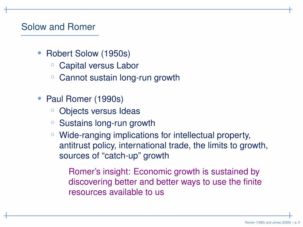
Solow and Romer
• Robert Solow (1950s)
◦ Capital versus Labor
◦ Cannot sustain long-run growth
• Paul Romer (1990s)
◦ Objects versus Ideas
◦ Sustains long-run growth
◦ Wide-ranging implications for intellectual property,antitrust policy, international trade, the limits to growth,sources of “catch-up” growth
Romer’s insight: Economic growth is sustained bydiscovering better and better ways to use the finiteresources available to us
Romer (1990) and Jones (2005) – p. 5

The Idea Diagram
Ideas → Nonrivalry →Increasing
returns
Long-run
growth
Problems withpure competi-
tion
ր
ց
Romer (1990) and Jones (2005) – p. 6

The Essence of Romer’s Insight
• Question: In generalizing from the neoclassical model to
incorporate ideas (A), why do we write the PF as
Y = AKαL1−α(*)
instead of
Y = AαKβL1−α−β
• Does A go inside the CRS or outside?
◦ The “default” (*) is sometimes used, e.g. 1960s
◦ 1980s: Griliches et al. put knowledge capital inside CRS
Romer (1990) and Jones (2005) – p. 7
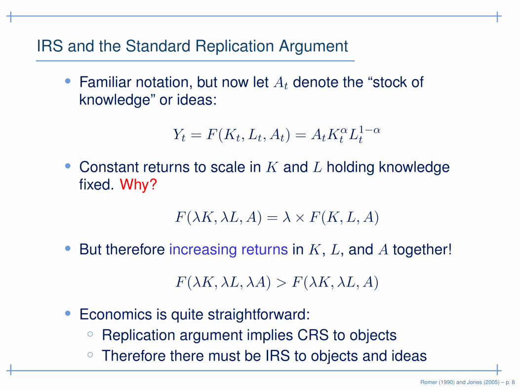
IRS and the Standard Replication Argument
• Familiar notation, but now let At denote the “stock ofknowledge” or ideas:
Yt = F (Kt, Lt, At) = AtKαt L
1−αt
• Constant returns to scale in K and L holding knowledgefixed. Why?
F (λK, λL,A) = λ× F (K,L,A)
• But therefore increasing returns in K, L, and A together!
F (λK, λL, λA) > F (λK, λL,A)
• Economics is quite straightforward:
◦ Replication argument implies CRS to objects
◦ Therefore there must be IRS to objects and ideas
Romer (1990) and Jones (2005) – p. 8

A Simple Model
Romer (1990) and Jones (2005) – p. 9
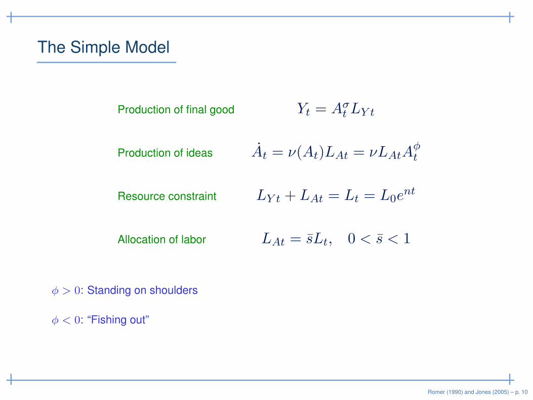
The Simple Model
Production of final good Yt = Aσt LY t
Production of ideas At = ν(At)LAt = νLAtAφt
Resource constraint LY t + LAt = Lt = L0ent
Allocation of labor LAt = sLt, 0 < s < 1
φ > 0: Standing on shoulders
φ < 0: “Fishing out”
Romer (1990) and Jones (2005) – p. 10

Solving
(1) Yt = Aσt LY t
(2) At = ν(At)LAt = νLAtAφt
(3) LY t + LAt = Lt = L0ent
(4) LAt = sLt, 0 < s < 1
Romer (1990) and Jones (2005) – p. 11
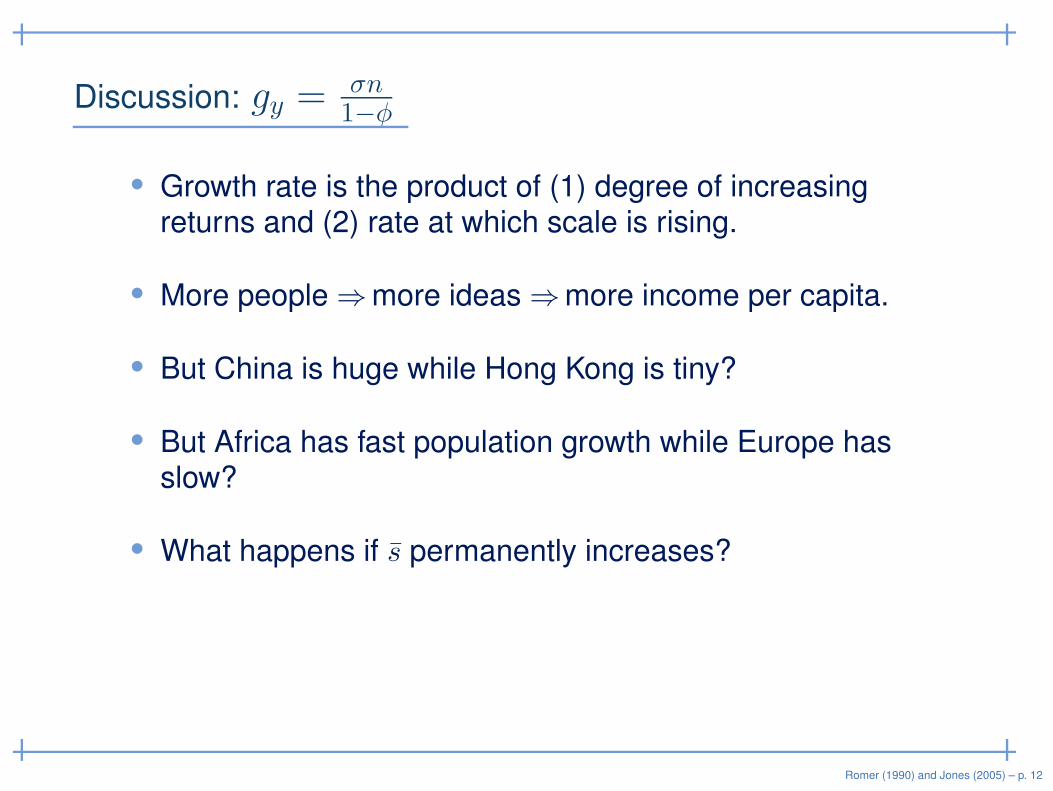
Discussion: gy =σn1−φ
• Growth rate is the product of (1) degree of increasingreturns and (2) rate at which scale is rising.
• More people ⇒more ideas ⇒more income per capita.
• But China is huge while Hong Kong is tiny?
• But Africa has fast population growth while Europe hasslow?
• What happens if s permanently increases?
Romer (1990) and Jones (2005) – p. 12
From IRS to Growth
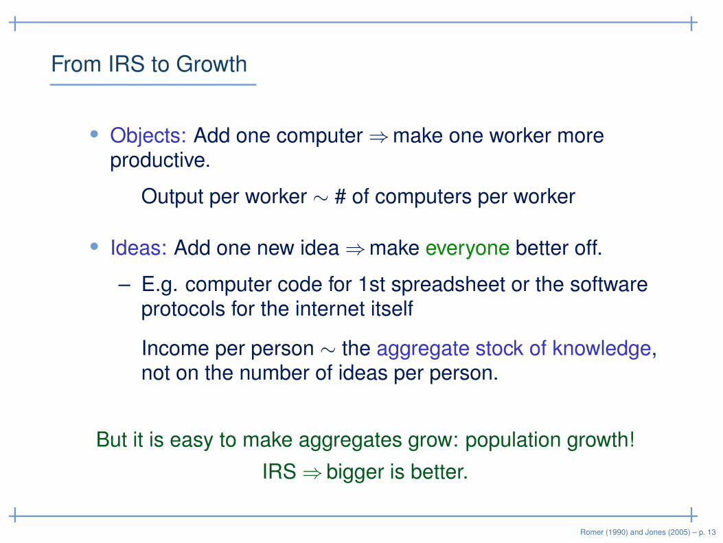
• Objects: Add one computer ⇒make one worker moreproductive.
Output per worker ∼ # of computers per worker
• Ideas: Add one new idea ⇒make everyone better off.
– E.g. computer code for 1st spreadsheet or the softwareprotocols for the internet itself
Income per person ∼ the aggregate stock of knowledge,not on the number of ideas per person.
But it is easy to make aggregates grow: population growth!
IRS ⇒bigger is better.
Romer (1990) and Jones (2005) – p. 13

Romer (1990) and Scale Effects
• Romer (1990) / Aghion-Howitt (1992) / Grossman-Helpman(1991) have φ = 1
AtAt
= νLAt = νsLt
• Policy effect: ↑ s raises long-run growth.
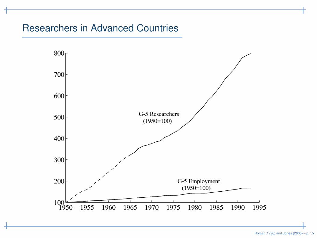
• Problem (Jones 1995): Growth in number of researchers (orpopulation) implies accelerating growth
◦ True over the very long run (Kremer 1993)
◦ But not in the 20th century for the United States.
Romer (1990) and Jones (2005) – p. 14
Researchers in Advanced Countries
Romer (1990) and Jones (2005) – p. 15

U.S. GDP per Person
Romer (1990) and Jones (2005) – p. 16

Scale Effects
• Strong versus weak (versus none)
◦ Strong: φ = 1 — scale affects the growth rate in LR
◦ Weak: φ < 1 — scale affects the level in LR
• Literature
◦ Young (1998), Peretto (1998), Dinopoulos-Thompson(1998), Howitt (1999); discussed in Jones (1999 AEAPP)
• No role for scale? What about nonrivalry?
Romer (1990) and Jones (2005) – p. 17

What happens if φ > 1?
Romer (1990) and Jones (2005) – p. 18
What happens if φ > 1?
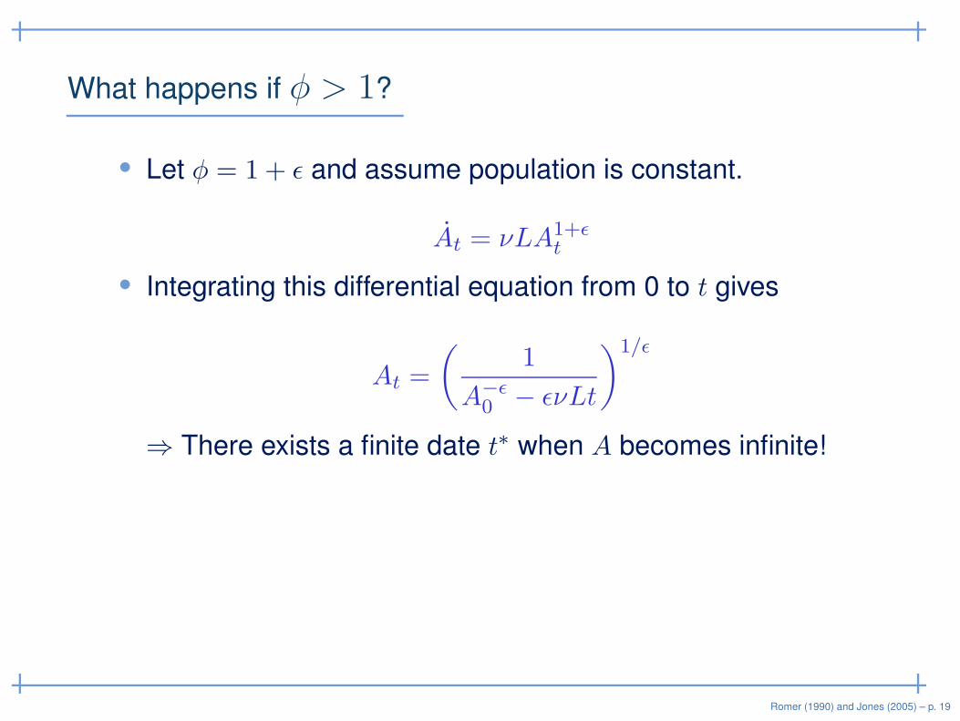
• Let φ = 1 + ǫ and assume population is constant.
At = νLA1+ǫt
• Integrating this differential equation from 0 to t gives
At =
(
1
A−ǫ0 − ǫνLt
)1/ǫ
⇒ There exists a finite date t∗ when A becomes infinite!
Romer (1990) and Jones (2005) – p. 19

The Full Romer Model
Romer (1990) and Jones (2005) – p. 20
Overview of Romer Model
• All of the key insights regarding nonrivalry and increasingreturns.
• In addition, a significant troubling question was how todecentralize the allocation of resources
◦ With increasing returns, why doesn’t one firm come todominate?
◦ Imperfect competition, a la Spence (1976), Dixit-Stiglitz(1977), and Ethier (1982, production side)
Romer (1990) and Jones (2005) – p. 21

The Economic Environment
Final good Yt =(
∫ At
0 xθit di)α/θ
L1−αY t , 0 < θ < 1
Capital Kt = It − δKt, Ct + It = Yt
Production of ideas At = νLλAtAφt , φ < 1
Resource constraint (capital)∫ At
0 xit di = Kt
Resource constraint (labor) LY t + LAt = Lt = L0ent
Preferences Ut =∫∞t Lsu(cs)e
−ρ(s−t) ds, u(c) = c1−ζ−11−ζ
Romer (1990) and Jones (2005) – p. 22

Allocating Resources
• Environment features
◦ 9 unknowns: Y,A, {xi}, LY , LA,K,C, I, L
◦ 6 1/2 equations (use∫
xitdi = K to get xt below)
Need 2 1/2 more equations to complete
• A rule of thumb allocation in this economy features
It/Yt = sK ∈ (0, 1)
LAt/Lt = sA ∈ (0, 1)
xit = xt for all i ∈ [0, At].
Romer (1990) and Jones (2005) – p. 23

Balanced Growth Path
A balanced growth path in this economy is a situation in which
all variables grow at constant exponential rates (possibly zero)
forever.
Romer (1990) and Jones (2005) – p. 24
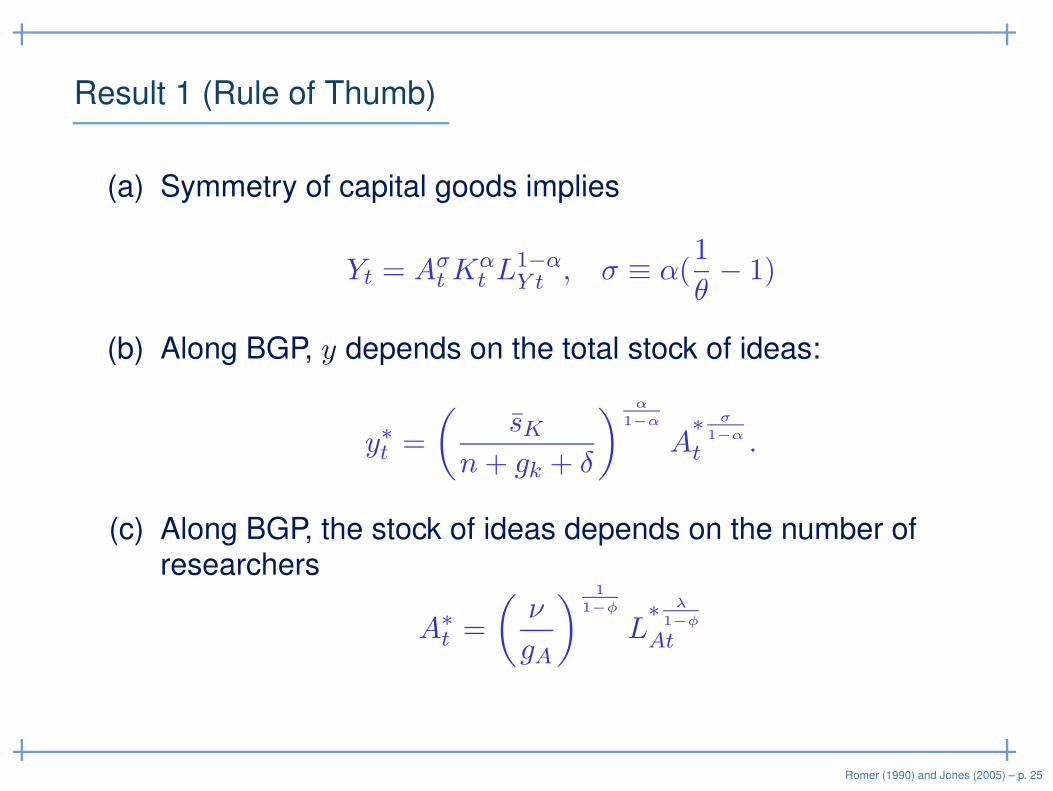
Result 1 (Rule of Thumb)
(a) Symmetry of capital goods implies
Yt = AσtKαt L
1−αY t , σ ≡ α(
1
θ− 1)
(b) Along BGP, y depends on the total stock of ideas:
y∗t =
(
sKn+ gk + δ
)α
1−α
A∗ σ
1−α
t .
(c) Along BGP, the stock of ideas depends on the number ofresearchers
A∗t =
(
ν
gA
)1
1−φ
L∗ λ
1−φ
At
Romer (1990) and Jones (2005) – p. 25
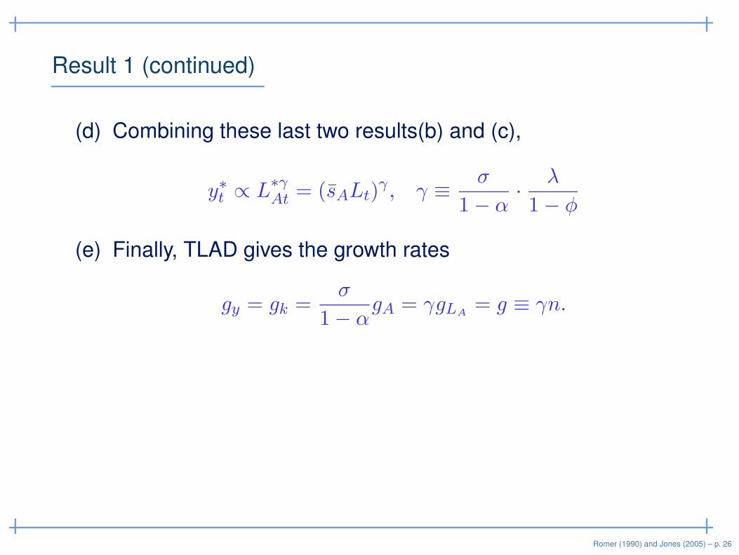
Result 1 (continued)
(d) Combining these last two results(b) and (c),
y∗t ∝ L∗γAt = (sALt)
γ , γ ≡σ
1− α·
λ
1− φ
(e) Finally, TLAD gives the growth rates
gy = gk =σ
1− αgA = γgLA
= g ≡ γn.
Romer (1990) and Jones (2005) – p. 26

The Optimal Allocation
• The optimal allocation features time paths {ct, sAt, {xit}}∞t=0
that maximize utility Ut at each point in time given theeconomic environment.
• Using symmetry of xit:
max{ct,sAt}
∫ ∞
0Ltu(ct)e
−ρt dt
subject to
yt = Aσt kαt (1− sAt)
1−α
At = ν(sAtLt)λAφt
kt = yt − ct − (n+ δ)kt
Romer (1990) and Jones (2005) – p. 27

The Maximum Principle in the Romer Model
• The Hamiltonian for the optimal allocation is
Ht = u(ct) + µ1t(yt − ct − (n+ δ)kt) + µ2tνsλAtN
λt A
φt ,
where yt = Aσt kαt (1− sAt)
1−α.
• First order necessary conditions
∂Ht/∂ct = 0, ∂Ht/∂sAt = 0
ρ =∂Ht/∂ktµ1t
+µ1tµ1t
, ρ =∂Ht/∂At
µ2t+µ2tµ2t
limt→∞
µ1te−ρtkt = 0, lim
t→∞µ2te
−ρtAt = 0
Romer (1990) and Jones (2005) – p. 28

Result 2 (Optimal Allocation)
(a) All of Result 1 continues to hold.
◦ Same long-run growth rate!
(b) Optimal consumption satisfies the Euler equation
ctct
=1
ζ
(
∂yt∂kt
− δ − ρ
)
(c) Optimal saving along BGP
sopK =α(n+ g + δ)
ρ+ δ + ζg
Romer (1990) and Jones (2005) – p. 29
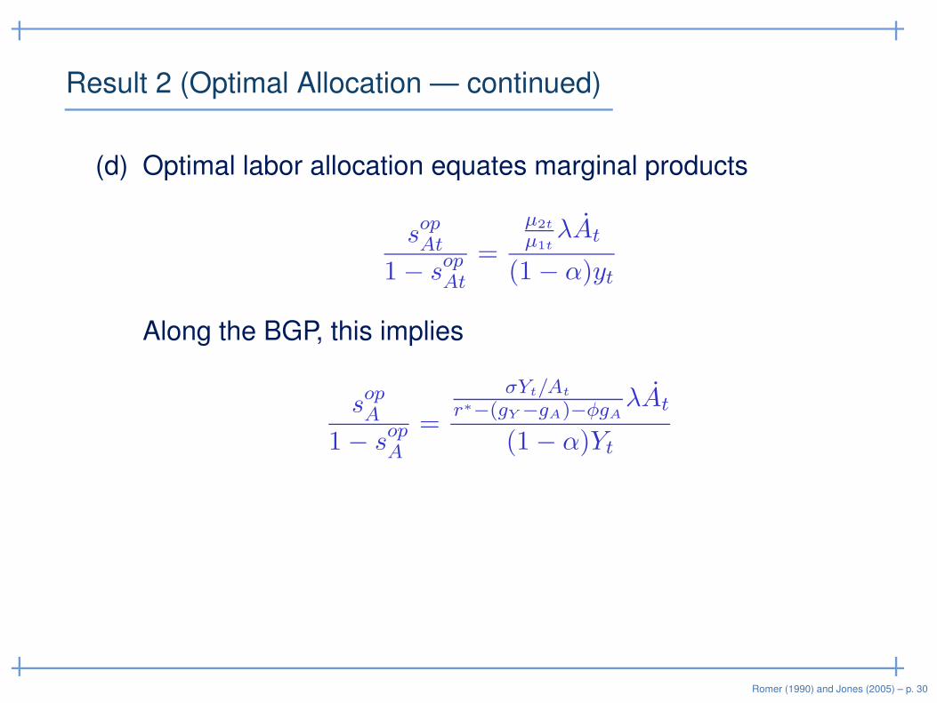
Result 2 (Optimal Allocation — continued)
(d) Optimal labor allocation equates marginal products
sopAt1− sopAt
=
µ2t
µ1tλAt
(1− α)yt
Along the BGP, this implies
sopA1− sopA
=
σYt/At
r∗−(gY −gA)−φgAλAt
(1− α)Yt
Romer (1990) and Jones (2005) – p. 30
Equilibrium in
the Romer Model
Romer (1990) and Jones (2005) – p. 31
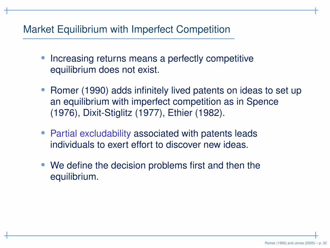
Market Equilibrium with Imperfect Competition
• Increasing returns means a perfectly competitiveequilibrium does not exist.
• Romer (1990) adds infinitely lived patents on ideas to set upan equilibrium with imperfect competition as in Spence(1976), Dixit-Stiglitz (1977), Ethier (1982).
• Partial excludability associated with patents leadsindividuals to exert effort to discover new ideas.
• We define the decision problems first and then theequilibrium.
Romer (1990) and Jones (2005) – p. 32
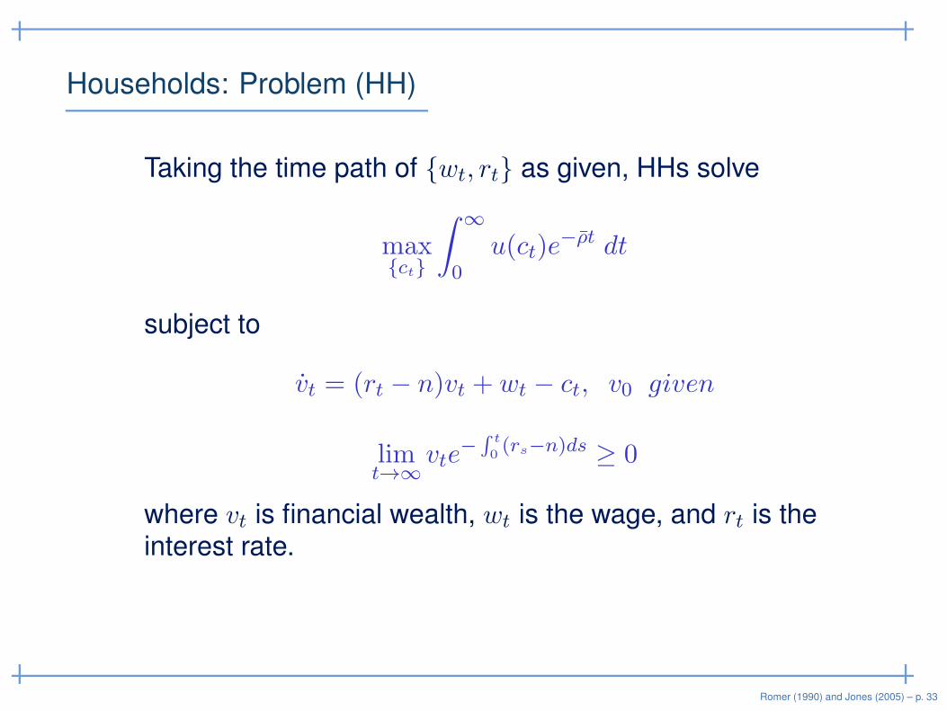
Households: Problem (HH)
Taking the time path of {wt, rt} as given, HHs solve
max{ct}
∫ ∞
0u(ct)e
−ρt dt
subject to
vt = (rt − n)vt + wt − ct, v0 given
limt→∞
vte−
∫t
0(rs−n)ds ≥ 0
where vt is financial wealth, wt is the wage, and rt is theinterest rate.
Romer (1990) and Jones (2005) – p. 33

Final Goods Producers: Problem (FG)
• Perfectly competitive
• At each t, taking wt, At, and {pit} as given, the
representative firm chooses LY t and {xit} to solve
max{xit},LY t
(∫ At
0xθit di
)α/θ
L1−αY t − wtLY t −
∫ At
0pitxitdi.
Romer (1990) and Jones (2005) – p. 34

Capital Goods Producers: Problem (CG)
• Monopolistic competition — a patent gives a single firm theexclusive right to produce each variety.
• At each t and for each capital good i, taking rt and x(·) asgiven, a monopolist solves
maxpit
πit ≡ (pit − rt − δ)x(pit)
where x(pit) is the (constant elasticity) demand from the
final goods sector for variety i — from the FOC in Problem(FG).
Romer (1990) and Jones (2005) – p. 35

Idea Producers: Problem (R&D)
• Perfectly competitive, seeing the idea production function as
At = νtLAt
• The representative research firm solves
maxLAt
PAtνtLAt − wtLAt
taking the price of an idea PAt, research productivity νt, andthe wage rate wt as given.
Romer (1990) and Jones (2005) – p. 36
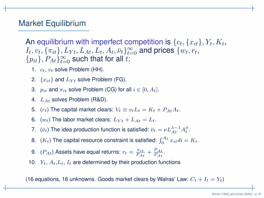
Market Equilibrium
An equilibrium with imperfect competition is {ct, {xit}, Yt,Kt,It, vt, {πit}, LY t, LAt, Lt, At, νt}
∞t=0 and prices {wt, rt,
{pit}, PAt}∞t=0 such that for all t:
1. ct, vt solve Problem (HH).
2. {xit} and LY t solve Problem (FG).
3. pit and πit solve Problem (CG) for all i ∈ [0, At].
4. LAt solves Problem (R&D).
5. (rt) The capital market clears: Vt ≡ vtLt = Kt + PAtAt.
6. (wt) The labor market clears: LY t + LAt = Lt.
7. (νt) The idea production function is satisfied: νt = νLλ−1
AtAφ
t .
8. (Kt) The capital resource constraint is satisfied:∫At
0xitdi = Kt.
9. (PAt) Assets have equal returns: rt =πitPAt
+ PAtPAt
.
10. Yt, At,Lt, It are determined by their production functions
(16 equations, 16 unknowns. Goods market clears by Walras’ Law: Ct + It = Yt)
Romer (1990) and Jones (2005) – p. 37

Result 3 (Market Equilibrium Allocation)
(a) All of Result 1 continues to hold:
◦ Same long-run growth rate!
(b) The same Euler equation characterizes consumption
ctct
=1
ζ(reqt − ρ)
Note: Since the growth rate is the same and the Eulerequation is the same, req = r∗ (steady state).
Romer (1990) and Jones (2005) – p. 38

Result 3 (Market Equilibrium — continued)
(c) Capital goods are priced with the usual monopoly markup:
peqit = peqt ≡1
θ(reqt + δ)
As a result, capital is paid less than its marginal product:
reqt = αθYtKt
− δ.
Same growth rate ⇒ same interest rate. Underpayingcapital leads to low K/Y :
seqK =αθ(n+ g + δ)
ρ+ δ + ζg= θsopK
Romer (1990) and Jones (2005) – p. 39

Result 3 (Market Equilibrium — continued)
(d) Free flow of labor equates marginal products
seqAt1− seqAt
=PAtAt
(1− α)Yt
Along BGP
seqA1− seqA
=
σθYt/At
req−(gY −gA)At
(1− α)Yt
Romer (1990) and Jones (2005) – p. 40

Compare sopA and seqA
seqA1− seqA
=
σθYt/At
req−(gY −gA)At
(1− α)Yt,
sopA1− sopA
=
σYt/At
r∗−(gY −gA)−φgAλAt
(1− α)Yt
Three differences:
• λ < 1: Duplication externality
• φ 6= 0: Knowledge spillover externality
• θ < 1: Appropriability effect
Equilibrium may involve either too much or too little research.
Romer (1990) and Jones (2005) – p. 41

Summary
• More people ⇒more ideas ⇒more per capita income(nonrivalry)
◦ Log-difference ⇒per capita growth is proportional topopulation growth, where proportionality measuresincreasing returns
• Long-run growth rate is independent of the allocation ofresources
◦ Subsides or taxes on research affect growth along thetransition path and have long-run level effects (likeSolow)
◦ In contrast, in Romer (1990), they lead to long-rungrowth effects
Romer (1990) and Jones (2005) – p. 42

Applications
Romer (1990) and Jones (2005) – p. 43
Several Applications of this Framework
1. Endogenizing population growth
2. Growth over the very long run
3. The linearity critique
4. Growth accounting
Romer (1990) and Jones (2005) – p. 44

1. Endogenizing Population Growth (Jones 2003)
• Let fertility be a choice variable in a Barro and Becker(1989) kind of framework.
◦ Converts this to a fully endogenous growth model
• But policy can have odd effects: a subsidy to research shiftslabor toward producing ideas but away from producing kids⇒ lower long-run growth!
• A recent reference on some intriguing issues that arisealong this line of research is Cordoba and Ripoll, “TheElasticity of Intergenerational Substitution, ParentalAltruism, and Fertility Choice” (REStud 2019)
Romer (1990) and Jones (2005) – p. 45

2. Growth over the Very Long Run
• Malthus: c = y = ALα, α < 1
◦ Fixed supply of land: ↑L ⇒ ↓c holding A fixed
• Story (Lee 1988, Kremer 1993):
◦ 100,000 BC: small population ⇒ ideas come very slowly
◦ New ideas ⇒ temporary blip in consumption, butpermanently higher population
◦ This means ideas come more frequently
◦ Eventually, ideas arrive faster than Malthus can reduceconsumption!
• People produce ideas and Ideas produce people
◦ If nonrivarly > Malthus, this leads to the hockey stick
Romer (1990) and Jones (2005) – p. 46
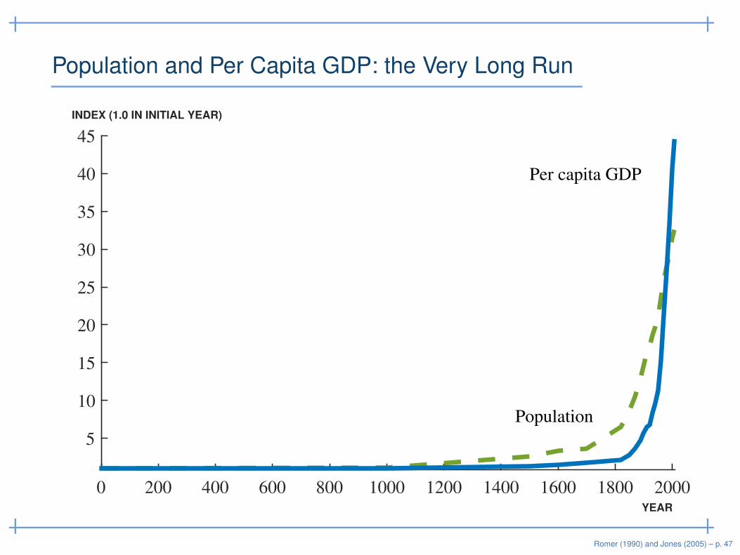
Population and Per Capita GDP: the Very Long Run
0 200 400 600 800 1000 1200 1400 1600 1800 2000
5
10
15
20
25
30
35
40
45
Population
Per capita GDP
YEAR
INDEX (1.0 IN INITIAL YEAR)
Romer (1990) and Jones (2005) – p. 47
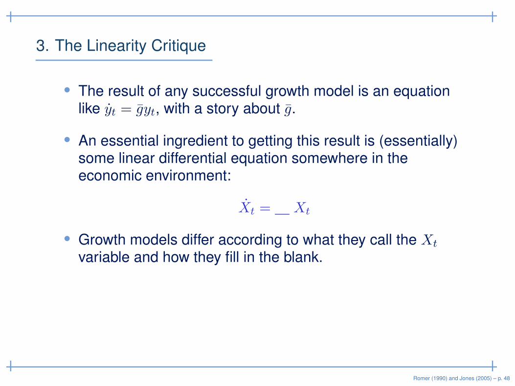
3. The Linearity Critique
• The result of any successful growth model is an equationlike yt = gyt, with a story about g.
• An essential ingredient to getting this result is (essentially)some linear differential equation somewhere in theeconomic environment:
Xt = Xt
• Growth models differ according to what they call the Xt
variable and how they fill in the blank.
Romer (1990) and Jones (2005) – p. 48
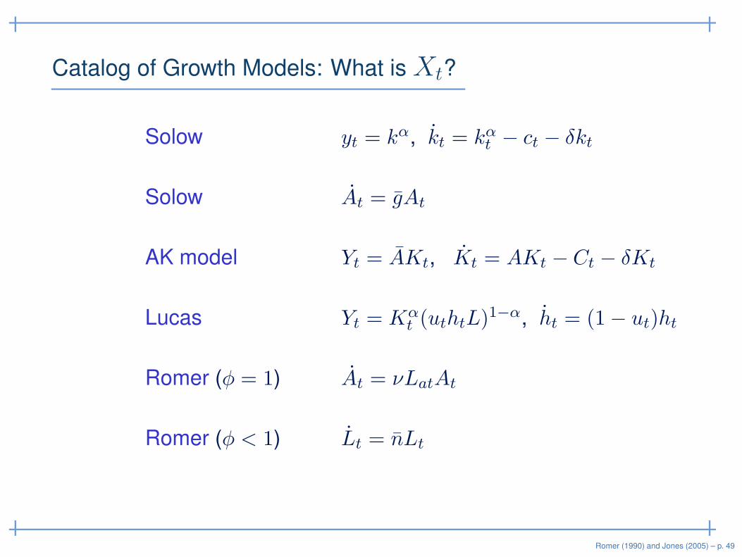
Catalog of Growth Models: What is Xt?
Solow yt = kα, kt = kαt − ct − δkt
Solow At = gAt
AK model Yt = AKt, Kt = AKt − Ct − δKt
Lucas Yt = Kαt (uthtL)
1−α, ht = (1− ut)ht
Romer (φ = 1) At = νLatAt
Romer (φ < 1) Lt = nLt
Romer (1990) and Jones (2005) – p. 49
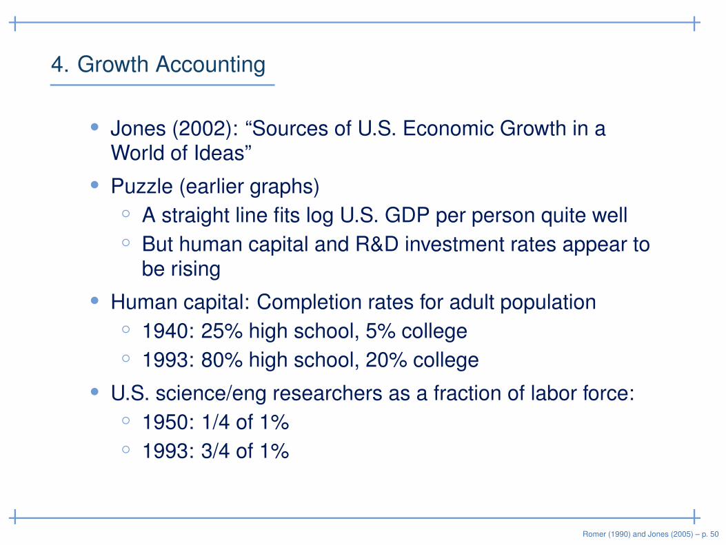
4. Growth Accounting
• Jones (2002): “Sources of U.S. Economic Growth in aWorld of Ideas”
• Puzzle (earlier graphs)
◦ A straight line fits log U.S. GDP per person quite well
◦ But human capital and R&D investment rates appear tobe rising
• Human capital: Completion rates for adult population
◦ 1940: 25% high school, 5% college
◦ 1993: 80% high school, 20% college
• U.S. science/eng researchers as a fraction of labor force:
◦ 1950: 1/4 of 1%
◦ 1993: 3/4 of 1%
Romer (1990) and Jones (2005) – p. 50

How to reconcile?
• Imagine a Solow model
◦ What happens if the investment rate grows over time?
• Same thing could be going on in an idea model with φ < 1◦ Only it is human capital and R&D investment rates that
rise
◦ Implication for the long run...
Romer (1990) and Jones (2005) – p. 51
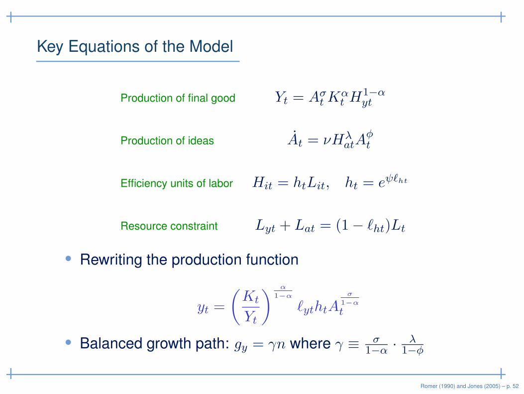
Key Equations of the Model
Production of final good Yt = AσtKαt H
1−αyt
Production of ideas At = νHλatA
φt
Efficiency units of labor Hit = htLit, ht = eψℓht
Resource constraint Lyt + Lat = (1− ℓht)Lt
• Rewriting the production function
yt =
(
Kt
Yt
)α
1−α
ℓythtAσ
1−α
t
• Balanced growth path: gy = γn where γ ≡ σ1−α · λ
1−φ
Romer (1990) and Jones (2005) – p. 52

Accounting for Growth (γ = 1/3), 1950–2007
• Educational attainment rises ≈ 1 year per decade. Withψ = .06 ⇒about 0.6 percentage points of growth per year.
• Transition dynamics are 80 percent of growth.
• “Steady state” growth is only 20 percent of recent growth!
• Numbers from “The Future of U.S. Economic Growth” (withFernald)
Romer (1990) and Jones (2005) – p. 53

Alternative Futures?
The stock of ideas, A
The shape of the idea production function, f(A)
The past
Today
Increasing returns
GPT"Waves"
Run outof ideas
Romer (1990) and Jones (2005) – p. 54