growth of alabama urban areas and its impact on changing

Growth of Alabama Urban Areas and Its Impact on Changing Environmental Dynamics

by

Mahjabin Rahman

A thesis submitted to the Graduate Faculty of Auburn University

in partial fulfillment of the requirements for the Degree of

Masters of Science in Geography

Auburn, Alabama August, 2014

Keywords: Urbanization, Alabama, Urban built-up,

Environmental Parameters, CA-Markov Model.

Copyright 2014 by Mahjabin Rahman

Approved by

Chandana Mitra, Chair, Assistant Professor of Geography

Luke Marzen, Professor of Geography Yingru Li, Assistant Professor of Geography

Sweta Byahut, Assistant Professor, School of Architecture

ii

Abstract

Urbanization plays a key role in modifying land cover and has widespread impact on the

environment. Atlanta has always been the focus of urban studies in south-eastern United

States. Little attention is given to urban areas smaller than Atlanta yet growing at an

alarming rate. Keeping this in view the focus of this study is on the eight cities of

Alabama which have encountered greater than 15 percent population increase between

1982 and 2010 and two large ones which have lost population. The main objectives are 1)

To determine the expansion of urban built-up areas of the ten cities over time (1982-

2010); 2) To examine temporal trends in temperature, precipitation, and air pollution for

the study areas (1980-2010) and understand the impact of urban built-up area on each;

and 3) To project future urban growth scenario (2040) for selective five cities using

Cellular Automata (CA) Markov model. Results revealed that there has been immense

expansion of urban built-up areas from1982 to 2010 due to population increase. Every

study area chosen there is an increasing trend in temperature and precipitation pattern.

Air quality has improvement in each city though expected otherwise. Regression results

revealed that variation in temperature, precipitation and PM 2.5 can be explained by urban

built-up expansion. The future growth model exposed that urban growth will take place

along the transportation routes mainly. The outcome of this research will help scientific

planning of cities in Alabama as well as implementing on other mid-sized cities globally.

iii

Acknowledgements

It would not have been possible to write this Master’s thesis without the help and support

of the kind people around me, to only some of whom it is possible to give particular

mention here.

Foremost, I would like to express my sincere gratitude to my advisor Dr. Chandana Mitra

for the continuous support of my MS study and research, for her patience, motivation,

enthusiasm, and immense knowledge. Her guidance helped me in all the time of research

and writing of this thesis. I could not have imagined having a better advisor and mentor

for my MS study. Besides my advisor, I would like to thank the members of my thesis

committee: Dr. Luke Marzen, Dr. Yingru Li and Dr. Sweta Byahut for their

encouragement, guidance, and insightful comments. My sincere thanks also go to Center

for Forest Sustainability, Auburn University. They have funded my work throughout my

MS degree here.

A special thanks to Dr. Ashraf Uddin, GPO, Department of Geology and Geography for

being so supportive on both academic a personal level, for which I am extremely grateful.

I also wanted to thank my fellow office mates: Holly Pak, Andrew Hug, Huixuan Li,

Mitch Carter, and Alyson Cederholm for their help, support, and encouragement. Last but

not the least; I would like to thank my family: my parents, my sisters and my husband for

supporting me and sending me so far for higher studies.

iv

Table of Contents

Abstract ............................................................................................................................... ii

Acknowledgements ............................................................................................................ iii

Table of Contents ............................................................................................................... iv

List of Tables ................................................................................................................... viii

Chapter 1: Introduction ....................................................................................................... 1

1.1 Introduction ............................................................................................................... 1

1.2 Urbanization and its Impact ...................................................................................... 4

1.3 Study Area ................................................................................................................. 6

1.4 Methodology ............................................................................................................. 9

1.5 Significance ............................................................................................................. 10

Chapter 2: Urban Built-up Expansion............................................................................... 12

2.1 Introduction ............................................................................................................. 12

2.2 Expansion of Urban Built-Up Areas ....................................................................... 15

2.2.1 Data Acquisition and Image Processing ........................................................... 15

2.2.2 Supervised Classification System for Urban Expansion .................................. 20

2.3 Results of Classification for all Ten Study Areas ................................................... 22

v

2.3.1 Birmingham-Hoover, Alabama ........................................................................ 23

2.3.2 Montgomery, Alabama ..................................................................................... 25

2.3.3 Mobile, Alabama .............................................................................................. 26

2.3.4 Dothan, Alabama .............................................................................................. 27

2.3.5 Decatur, Alabama ............................................................................................. 29

2.3.6 Huntsville and Madison, Alabama ................................................................... 31

2.3.7 Auburn, Alabama.............................................................................................. 32

2.3.8 Tuscaloosa, Alabama ........................................................................................ 34

2.4 Accuracy Assessment of Classified Images ............................................................ 35

2.5 Summary ................................................................................................................. 36

Chapter 3: Urbanization and Impact on Environment ...................................................... 38

3.1 Introduction ............................................................................................................. 38

3.2 Temporal Trends of Environmental Parameters ..................................................... 39

3.3 Relationship between Environmental Parameters and Urban Built-up Area .......... 40

3.4 Data and Data Sources ............................................................................................ 42

3.5 Methodology ........................................................................................................... 42

3.5.1 MK Trend Test ................................................................................................. 42

3.5.2 Multiple Linear Regression .............................................................................. 44

3.6 Results ..................................................................................................................... 46

3.6.1 Trend Analysis using MK Trend Test .............................................................. 46

vi

3.6.2 Multiple Linear Regressions ............................................................................. 52

3.7 Summary ................................................................................................................. 55

Chapter 4: A Peek into Future Urban Growth .................................................................. 56

4.1 Introduction ............................................................................................................. 56

4.2 Future Urban Growth using CA Markov Model ..................................................... 57

4.2.1 Cross Classification of Two Images ................................................................. 58

4.2.2 Markov Chain Analysis .................................................................................... 59

4.2.3 Cellular Automata (CA) ................................................................................... 60

4.2.4 CA Markov Model............................................................................................ 61

4.2.5 Model Validation .............................................................................................. 62

4.3 Results ..................................................................................................................... 62

4.3.1 Transition Probability Matrix ........................................................................... 62

4.3.2 Urban Built-Up Area Prediction for the year 2040 .......................................... 64

4.3.3 Validation of CA-Markov Model ..................................................................... 69

4.4 Summary ................................................................................................................. 70

Chapter 5: Conclusion and Summary ............................................................................... 72

5.1 Urban Built-up Expansion ....................................................................................... 72

5.2 Environmental Parameters ...................................................................................... 74

5.3 Future Urban Built-up Expansion ........................................................................... 76

5.4 Conclusion and Significance ................................................................................... 77

vii

References ......................................................................................................................... 80

Appendices ........................................................................................................................ 87

viii

List of Tables

Table 1.Growth (increase and decrease) in population for the ten cities in Alabama from 1980 to 2010. ...................................................................................................................... 7 Table 2. Information of the Satellite Image used in this Study. ....................................... 17

Table 3. Image Classification Scheme. ............................................................................. 21

Table 4. Land Use Land Cover Statistics for Birmingham- (1982-2010). ....................... 25

Table 5. Land Use Land Cover Statistics for Hoover (1982-2010). ................................. 25

Table 6.Land Use Land Cover Statistics for Montgomery (1982-2010). ......................... 26

Table 7. Land Use Land Cover Statistics for Mobile (1982-2010). ................................. 27

Table 8.Land Use Land Cover Statistics for Dothan (1982-2010). .................................. 29

Table 9.Land Use Land Cover Statistics for Decatur (1982-2010). ................................. 30

Table 10. Land Use Land Cover Statistics for Huntsville (1982-2010). .......................... 32

Table 11. Land Use Land Cover Statistics for Madison (1982-2010). ............................. 32

Table 12. Land Use Land Cover Statistics for Auburn (1982-2010). ............................... 33

Table 13. Land Use Land Cover Statistics for Tuscaloosa (1982-2010). ......................... 35

Table 14. Accuracy Assessment and Kappa Statistics of Classified Image. .................... 36

Table 15 : Variables and their Indicators .......................................................................... 45

Table 16. Mann-Kendall Summary of Temperature Data for the Ten Study Areas (1980-2010). ................................................................................................................................ 48 Table 17. Mann-Kendall Summary of Precipitation Data for the Ten Study Areas (1980-2010). ................................................................................................................................ 50 Table 18. Mann-Kendall Summary of Ozone Data for the Ten Study Areas ................... 51

ix

Table 19. Mann-Kendall Summary of PM2.5 Data for the Ten Study Areas .................... 52

Table 20. Regression Results for Temperature. ................................................................ 53

Table 21. Regression Results for Precipitation. ................................................................ 54

Table 22. Regression Results for PM 2.5. .......................................................................... 55

Table 23. Transition Probability Matrix of Markov Model for Five Study Areas. .......... 63

Table 24. Factors Controlling Future Growth (derived from MCE). ............................... 65

Table 25. Predicted Urban Built-up by 2040. ................................................................... 66

Table 26. Net Addition of Urban Built-up from 1982-2010 for Ten Study Areas. .......... 73

x

List of Figures

Figure 1. Area of 10 Study Areas. ...................................................................................... 7

Figure 2. Location of Ten Study Areas (Map created by Mahjabin Rahman) .................. 8

Figure 3. 2010 Census Urbanized Area Reference Map for 10 Study Areas. .................. 18

Figure 4. Landsat Full Scene (Left) Compare to AOI (Right) for 10 Study Areas .......... 19

Figure 5. Urban Built-up Expansion for Birmingham (left) and Hoover (right). ............. 24

Figure 6.Urban Built-up Expansion for Montgomery. ..................................................... 26

Figure 7. Urban Built-up Expansion for Mobile. .............................................................. 27

Figure 8.Urban Built-up Expansion for Dothan. .............................................................. 28

Figure 9. Urban Built-up Expansion for Decatur. ............................................................. 30

Figure 10.Urban Built-up Expansion for Huntsville (left) and Madison (right). .............. 31

Figure 11. Urban Built-up Expansion for Auburn. ........................................................... 33

Figure 12. Urban Built-up Expansion for Tuscaloosa. ..................................................... 34

Figure 13. Urban Built-up Area Statistics (1982-2010) .................................................... 36

Figure 14. Screen Shot of MK test in Addinsoft’s XLSTAT 2013. ................................. 44

Figure 15. Multiple Linear Regression in Excel. .............................................................. 46

Figure 16. Temporal Trends for Madison, Alabama (1980-2010). .................................. 47

Figure 17. Flow diagram showing this study’s CA-Markov Model Design..................... 59

Figure 18. Predicted Urban Built-up Expansion for Madison, 2040. ............................... 67

Figure 19. Predicted Urban Built-up Expansion for Birmingham-Hoover, 2040. ............ 68

xi

Figure 20. Predicted Urban Built-up Expansion for Hoover, 2040. ................................. 68

Figure 21. Predicted Urban Built-up Expansion for Mobile, 2040. .................................. 69

Figure 22. Predicted Urban Built-up Expansion for Auburn, 2040. ................................. 69

xii

List of Abbreviations

US United States

UN United Nations

LULCC Land Use Land Cover Change

LULC Land Use Land Cover

MK Mann-Kendall

MSA Metropolitan Statistical Area

CA Cellular Automata

GIS Geographic Information System

TM Thematic Mapper

IR Infra-Red

USGS United States Geological Survey

GLOVIS Global Visualization Viewer

AOI Area of Interest

AL Alabama

O3 Ozone

PM 2.5 Particulate Matter 2.5

NWS National Weather Service

NCDC National Climatic Data Center

EPA Environmental Protection Agency

xiii

MCE Multi Criteria Evolution

AHP Analytic hierarchy process

IPCC Intergovernmental Panel on Climate Change

SIP State Implementation Plan

H0 Null Hypothesis

H1 Alternative Hypothesis

Rst Raster

Img Image

1

Chapter 1: Introduction

1.1 Introduction

The coming decades will see a steady increase in urban population globally. A United

Nations report mentions that the wor ld population i s expected to be on the order of

70 percent urban by 2050 (UN 2007). In case of United States (US) urbanization

developed over the last two centuries from being a major rural, agricultural nation into an

industrial one. In US the urbanization process was slow with the nation becoming an

urban-majority between 1910 and 1920 (US Census 2010 a). At present, just over four

fifths of the US citizens live in urban areas, and the number is still on the rise (US census

2010 a).

Narrowing it down to Alabama, within the group of southeastern states of US,

it is the only one where, between 2000 and 2009, more than half of the growth (53

percent) resulted from natural increase ( number of births minus number of deaths)

(Georgia Office of Planning and Budget, 2010). A l s o , Alabama is one of the slowest

growing states in the US (30th in rank) on the basis of overall population. During the

1990s, the population in Alabama grew by 10.1 percent whereas nationally,

population increased by 13.1 percent. Particularly significant was in 2010

when the nation’s population increased by 9.7 percent whereas in Alabama it

increased by only 0.48 percent (US census 2010a).

2

Though the state of Alabama shows slow population growth, individual cities

within Alabama tells a very different story. Over past few decades, the population

of major cities in Alabama has shown huge increases with the exception of Birmingham

a n d Mobile. Madison, H o o v e r and Auburn have shown significant growth over time

in past 30 years too. Population increase creates pressure on the infrastructure and

dynamics of the city and to accommodate the growing population there is naturally an

increase in urban built-up area (Lambin et al 2001, Cohen 2006). And the rate at which

urban areas are growing is of much concern to both social and natural scientists since

urban area has an impact on human health (Jackson 2003) as well as on surrounding

physical environment (Oke 1973). So in this study as a proxy to growing population and

its impacts on landuse, urban built-up area increase over time will be considered and

quantified.

Presently most of the urban studies focus on large sized cities across the world

like Atlanta, New York, Tokyo, Kolkata and Dhaka (Yang 2002,Islam and Ahmed

2011, and Mitra et al 2012) thus ignoring the medium sized cities, which have the most

growth potential with significant ecological footprint on the face of the earth. For the

same reason this research mainly focuses on medium sized and small sized cities which

have the potential of both horizontal and vertical growth. Based on population, the US

Census categorized all medium sized cities ranking them between 101 and 200 compared

to all sizes (US Census 2010a). The populations of these medium-sized cities ranged

from 98,000 to 210,000 in 2010. Based on these statistics, there are one large sized

(Birmingham: rank 100) and three mid-sized cities in the State of Alabama

(Montgomery: rank 105, Mobile: rank 120, and Huntsville: rank 126). Rest of them fall

3

in small-sized categories above 200. A study revealed that medium-sized cities grew

faster in population than the largest ones (Detroit, Cleveland, Pittsburg, Saint Louis,

New Orleans) which lost more than 20 percent of their population during the 1990s in

the US (Vey and Forman 2002). The study also revealed fastest growing cities were in

the south and western part of US (Vey and Forman 2002). Echoing the above findings

the major Alabama cities are losing population whereas medium sized ones are gaining

population rapidly in a short period of time (Table 1). Birmingham city and Mobile

city have slower growth (25.4 percent and 2.7 percent population were lost respectively

for each stated urban areas from 1980 to 2010) compared to other small cities like

Hoover and Madison (more than 300 percent and 900 percent growth shown for

respective cities from 1980 to 2010) (data calculated from US census 2010a).

Rapid urbanization in the form of population increase has led to an increase in

built-up area and impervious surfaces, increased greenhouse gas emissions and more

anthropogenic activities which are argued to be detrimental to the delicate yet complex

environmental-climate system of the Earth (Yang et al 2003). The ability of an urban

area to generate an effect on environment is now a well-accepted fact (Oke 1973, Han et

al 2013). A relationship has been found between intensity of this effect and size of urban

areas (in terms of population). It is revealed that larger the areas, the higher the impact

on environment (Oke 1973). Han et al (2013) also mentioned that urban areas affect the

spatial distribution and amount of precipitation in south-eastern Brazil.

Keeping this in mind, this research focuses on understanding the dynamics of

urban built-up expansion in Alabama and changing urban environment. Here urban

built-up area is defined as the area confined by the built-up impervious surface in a city

4

as described in remote sensing literature (Yang et al 2003). The research has delved on

urban built-up expansion and whether it has modified the various environmental

parameters. In particular, the project would have sought to address the following

objectives:

1. To determine the expansion of urban built-up areas over time (1982-2010), for ten

cities using supervised classification.

2. To examine temporal trends in temperature, precipitation, and air pollution

(concentration of ozone and particulate matter 2.5 in air) in the study region (using

Mann-Kendall trend test) for 1980-2010 and to understand the impact of urban built-up

expansion on environmental parameters (using multiple linear regression).

3. Project future urban growth scenario (2040) for selective five cities using cellular

automata (CA) Markov model.

1.2 Urbanization and its Impact

The global population has become concentrated in cities (UN 2007). Over the last

hundred years, depending on the region, the world has rapidly become an urban one, with

detrimental consequences caused by changes in population distribution. The share of

world population that lives in urban areas has increased from 5 percent in 1900 to over 50

percent today with the largest proportion of this urban population in developing countries

(Maktav et al 2005). Urbanization is accompanied by artificial changes in land use land

cover change (LULCC). Urban areas are composed of numerous man-made structures

and urban surfaces covered with materials such as concrete and asphalt (Han et al 2013).

5

In the United States, there was a 34 percent increase in the amount of land

devoted to urban and built-up uses between 1982 to 1997 (Alig et al 2003). Their main

source of data was United States Department of Agriculture. According to the 2010 (c)

census, 80.7 percent of US population lives in urban areas, a substantial increase from

73.7 percent in 1980 (US census, 1995d). Statistical projections (estimated regression

model coefficients) suggest continued urban expansion over the next 25 years, with the

magnitude of increase varying regionally (Alig et al 2003). The developed area within

US is projected to increase by 79 percent, raising the proportion of the total land base in

the US that is developed from 5.2 to 9.2 percent (Alig et al 2003). Here urban and built-

up areas are defined as land uses consisting of residential, industrial, commercial, and

institutional land as well as several public infrastructure land use categories such as

railroads, landfills etc. (Alig et al 2003).

Many studies reveal that urbanization has several impacts on environmental

parameters. Some studies have been done in India (precipitation), Turkey (relative

humidity), Nigeria (temperature) and US (air quality). These studies indicate that

increasing trend in urbanization has a positive relationship on environmental parameters

(temperature and precipitation). (Tayanc and Toros 1997, Mitra et al 2011, Babatola

2013).

The benefits of urbanization are increasingly measured against ecosystem

impacts, including degradation of air and water quality and others (Squires 2002; Yuan et

al 2005). Large cities across the US have seen marked increases in urban growth and the

associated impacts of environmental degradation (Yuan et al 2005). Research has

highlighted urbanization effects on different environmental parameters, for instance,

6

temperature, precipitation, and air quality (Oke 1973, Tayanc and Toros 1997,

Superczynski and Christopher 2011).

1.3 Study Area

In this research, the study areas have been selected on the basis of city population from

2010 census data (US census 2010 b), the cities which have had a population growth

greater than 15 percent from 1980 to 2010 (table 1, figure 2). This research did not

consider the Metropolitan Statistical Area (MSA) population. The main reason behind

this is to highlight how the small sized cities like Hoover and Madison have been

growing in the recent past. If MSA would be considered then Madison and few other

smaller cities which are not yet metro areas would not be considered under the scope of

this research. The two exceptions showing negative population growth in recent past are

Birmingham and Mobile cities. Their inclusion in the study will help in understanding

whether population decline also influences urban built-up.

Figure 1 shows the areal extent of the ten study areas and figure 2 shows their

spatial coverage spread over the whole Alabama state. Table 1 indicated that major

cities like Birmingham and Mobile are growing slowly (25.4 percent and 2.7 percent

population were lost respectively for each stated cities from 1980 to 2010) compared to

other cities like Hoover and Madison (more than 300 percent and 900 percent growth

shown for respective cities from 1980 to 2010) (data calculated from US census

2010a).

For classification purpose in this study, the study areas are consisted of 2010

urbanized areas reference map in the state of Alabama (US census 2010 b) for

7

supervised classification.

Table 1.Growth (increase and decrease) in population for the ten cities in Alabama from 1980 to 2010.

Source: United States Census Bureau, 2010 a.

Source: United States Census Bureau, 2010a.

Figure 1. Area of 10 Study Areas.

Study Areas (Based on city population) Population Population Change, 1980 to 2010

1980 2010 Number Percent

Birmingham 284413 212237 -72176 -25.4 Montgomery 177852 205764 27912 15.7 Mobile 200452 195111 -5341 -2.7 Huntsville 142513 180105 37592 26.4 Tuscaloosa 75211 90468 15257 20.3 Hoover 19792 81619 61827 312.4 Dothan 48750 65496 16746 34.3 Decatur 42002 55683 13681 32.6 Auburn 28471 53380 24911 87.5 Madison 4057 42938 38881 958.4

8

Figure 2. Location of Ten Study Areas (Map created by Mahjabin Rahman)

9

1.4 Methodology

Various geospatial methodologies have been used in different studies to quantify and

analyze impacts of land use land cover change on the environment. In this study three

different methods have been approached to fulfill the objectives.

Chapter 2 deals with determination of urban expansion. Remote sensing

techniques to study urban expansion are discussed in this chapter. Image analysis of

Landsat 5 Thematic Mapper (TM) imagery methods utilizing supervised classification

using ERDAS Imagine 13 software has been conducted here. This technique is used to

determine the urban expansion of all study areas over 28 years (1982-2010).

Chapter 3 looks at the change of environmental parameters over time (1980-

2010).This research has been selected two weather parameters ( temperature,

precipitation) and two air quality parameters ( PM 2.5 and Ozone). Man-Kendall statistical

technique was used to test the non-parametric variables which require that data should be

independent and can tolerate outliers in the dataset (Onoz and Bayazit 2003). To

investigate the relationship between urban built-up and environmental parameters,

multiple linear regression has also been demonstrated in this chapter. It is important to

highlight that analysis of urban expansion has been done from 1982 to 2010, whereas

trends of environmental parameters has been analyzed from 1980 to 2010 based on data

availability.

In chapter 4 Cellular Automata (CA) Markov is used to forecast urban expansion

for 2040 for five urban areas (Birmingham, Hoover, Madison, Mobile, and Auburn).

These urban areas were chosen based on their significance. Birmingham and Mobile,

though largest have been losing population and the others are gaining population. This

10

model is developed in the Geographic Information System (GIS) environment and

provides spatial outputs which may help to manage and evaluate urban areas in

development scenarios.

Chapter five summarizes the findings of this research highlighting the

significance of the study in the perspective of the dynamic nature of urban areas and their

influence on environment and the people who live in them.

1.5 Significance

This study will be a unique synergy of urban land cover dynamics and environmental

parameters. Future prediction and managing urban growth requires rigorous use of

technologies and methods in order to produce accurate mapping of land use and land

cover. Remote sensing imagery will provide geographic and temporal overview of urban

development in Alabama. Various statistical techniques (Mann-Kendall test and multiple

linear regression) will provide a quantitative analysis of the environmental parameters:

how their temporal trends are changing with time and relationship between urban

expansion and environmental parameters. The principal objective to use urban growth

model is evaluating possible future paths of development on various urban sectors.

It is important to analyze not only the urban built-up expansion but also see how it

influences precipitation, temperature, air quality, water availability, health etc. which

could be compromised in the future with population pressure in the urban areas. Extreme

events like heat waves, tropical cyclones, and rainfall events are predicted to be on the

rise in recent decades (Peterson et al 2013) and thus it is very important to understand the

dynamics of urban areas and be prepared for adapting and mitigating the impacts. As it is

11

well known that more than half of the world’s population lives in urban areas (Population

Reference Bureau 2012) so their resource intensive living patterns must be having a large

impact on local environment and eventually on the global environment as well. Thus it is

very important to manage urban areas in a sustainable way and be environmentally

conscious and be conservative on energy usage.

The significance of this study also lies in shifting focus from large cities to

smaller cities which have the maximum potential to grow in future. It is better to be

prepared ahead of time to cope with the local and regional changes.

By using ten cities in the study, the findings will establish a possible link between

urban built-up expansion and changing patterns of environmental parameters. The

findings of this research will provide a better understanding of what we are expecting in

our future and what we can do to adapt and mitigate the impacts.

12

Chapter 2: Urban Built-up Expansion

2.1 Introduction

It is important to understand what urbanization is and why it is important in present

scenarios. Urbanization is a dynamic process which changes patterns with increasing

number of people coming to live in urban areas. It predominantly results in the physical

growth of urban areas, horizontal or vertical (UN 2007). It is also important to quantify

this conversion from natural to built-up environments in urban areas as it can profoundly

impact the land atmosphere dynamics locally as well as regionally.

Determination of urban expansion involves procedures of monitoring and

mapping which require robust methods and techniques (Yang 2002). Traditional methods

for gathering demographic data, censuses, and maps using samples are limited for urban

management purposes because updating process is time and labor intensive (Maktav

2005). Also traditional survey and mapping methods cannot deliver the necessary

information in timely and cost-effective manner. These methods are also time consuming,

contain errors, and are not appropriate here. Given their technological challenges, remote

sensing technologies are increasingly becoming popular in urban land use change

research (Civco et al 2000; Yang 2002, Araya and Cabral 2010). The basic premise of

using remote sensing is that it can identify change between two or more time periods

(Roy 2000; Shalaby and Tateishi 2007). Roy (2000); Shalaby, and Tateishi (2007) also

13

note that remote sensing and GIS provide opportunities for integrated analysis of spatial

data.

Supervised and unsupervised classifications are two traditional pixel-based

methods of analyzing remotely sensed data (Maktav et al 2005). In supervised

classification, a user selects training sites for desired classes and then pulls them from the

image using a statistical algorithm, while in unsupervised classification, the software

statistically groups pixels into similar clusters then the user assigns the clusters to a class

by referencing the imagery used for the classification (Campbell 2002). Pixel-based

classification is easy to use and quite successful in classifying land cover of a

homogenous nature like closed forest (Whiteside and Ahmad 2005).

A large body of research exists in the field of assessing urban extent using remote

sensing and GIS techniques (Maktav et al 2005). According to Maktav et al (2005)

remote sensing – as a technique for observing the surface of the Earth from different

platforms – and Geographic Information Systems (GIS) can mitigate the problems of

traditional field-based data collection methods by providing up-to-date spatial

information over large expenses of territory. Moreover, remote sensing data can identify

LULCC between two or more time periods effectively (Roy 2000; Shalaby and Tateishi

2007).

Many researchers also used remote sensing and GIS techniques to understand

urban areas across the world. Lambin and Ehrilch (1997) used ten years of data to assess

and analyze land cover changes in the African continent between 1982 and 1991. Another

study was conducted in the lake regions of central Ethiopia using aerial photographs

14

dated 1972 and 1994 from Landsat thematic mapper (TM) images (Ferrari 2000; Shalaby

and Tateishi 2007). Ram and Kolakar (1993) also studied land use changes in India

(Shalaby and Tateishi 2007). In addition a supervised classification was done for the

Northwestern coast of Egypt by Shalaby and Tateishi (2007) to delineate LULCC.

Here in the US many studies were conducted to understand LULCC using remote

sensing. Xiaojun Yang (2002) monitored the urban spatial growth in the Atlanta

metropolitan area in 2002 using an unsupervised classification system from Landsat TM

data between 1973 and 1999. According to Yang, remote sensing and GIS offer the best

way to manage urbanization because these techniques provide accurate spatial

information. Similarly Yuan et al (2005) studied land cover classification and change

analysis of the twin cities in Minnesota. They used a supervised-unsupervised hybrid

approach to classify images. The result has proven the potential of multi-temporal

Landsat data to provide an accurate map of landscape changes and valuable statistics

documenting change over time (Yuan et al 2005). In addition they also examined the

relationship between population growth and growth in urban land area through Landsat-

derived change maps.

In Alabama, Trousdale (2010) conducted a study of Birmingham and Hoover

using supervised classification. He measured the expansion of urban sprawl over a 34

year period (1974-2008). The results reveal that over the study period there was a steady

decline in forests, agricultural lands, and green space and an expansion of urban and

residential land-use/land-cover in the metropolitan area in the form of built-up area.

15

2.2 Expansion of Urban Built-Up Areas

Remotely sensed image analysis is a challenging task. One popular and commonly used

approach for image analysis is image classification. The purpose of image classification

is to label the pixels in the image with meaningful information of the real world (Jensen

et al 2001; Matinfar 2007). Through classification of digital remote sensing images,

thematic maps bearing the information such as land cover types; vegetation types etc. can

be obtained (Tso et al 2001; Matinfar 2007).

2.2.1 Data Acquisition and Image Processing

Landsat Thematic Mapper (TM) imagery has been used for this study. The Landsat TM

is a technologically advanced sensor integrating multiple radiometric, spectral, and

geometric enhancements from its predecessors. The imagery provides data in seven

bands of the spectrum—visible spectrum (blue, green, red), near-IR, 2 mid-IR bands, and

thermal. The wavelength location and range of the TM bands have been enhanced from

its predecessors, improving the spectral differentiability of surface features of Earth

(Lillesand et al 2004). It has a spatial resolution of 30x30 m, temporal resolution of 16

days and radiometric resolution of 8 bits.

For urban land cover classifications with Landsat TM, the most useful bands are

visible, near infrared, and middle-infrared, because combination of these bands

highlights LULC in a better way (Jensen 2007). TM images were obtained for four

decades -1982s, 1990s, 2000s and 2010s from the United States Geological Survey

(USGS) Global Visualization Viewer (GLOVIS) for ten different study areas of

Alabama (http://glovis.usgs.gov/).

http://glovis.usgs.gov/

16

Raw remotely sensed image data are full of geometric, radiometric, and

atmospheric flaws caused by the curved shape of the Earth, the imperfectly transparent

atmosphere, daily and seasonal variations in the amount of solar radiation received at the

surface. USGS offers correction of these flaws. Geometric flaws are corrected by process

rubber sheeting (Lillesand and Kiefer 1994). It involves stretching and warping an image

to georegister control points shown in the image to known control point locations on the

ground. There are several numerous radiometric correction techniques, including Earth-

sun distance corrections, and sun elevation corrections. Atmosphere errors are corrected

by haze compensation (Lillesand and Kiefer 1994).

Temporal resolution became an issue while trying to find adequate satellite

imagery for analysis. Acquiring anniversary images is the best option with

corresponding season, month, and preferably week for each year. Many times this is not

possible because of the times that the sensor system passes over the particular area.

However, with classification methods a user can account for seasonal differences as

images are classified independently. Another problem is weather; when there is a

thunderstorm or just cloud cover it is impossible to produce an accurate urban land cover

classification. Many times anniversary dates are impossible, and the logical alternative

would be to find images of the area in the same month or season (Jensen 2007). For this

study it was possible to acquire satellite data close to anniversary dates (Table 2).

17

Table 2. Information of the Satellite Image used in this Study.

The downloaded images covered a larger area than actual urban extent, so a

subset of the required area was needed. The study area for each urban area is a chosen

‘area of interest’ (AOI) around the most recent boundary of census bureau defined

urbanized area (figure 3) (US census 2010b).

Study Area Path Row Date 1982 1990 2000 2010

Auburn 19 37 December January January January Dothan 19 38 December January January January Tuscaloosa 27 37 June June June June Mobile 21 39 January February March February Huntsville 20 36 April April April April Madison 20 36 April April April April Decatur 21 36 October November November November Birmingham 20 37 December December January December Hoover 20 37 December December January December Montgomery 20 38 March March March March

18

Figure 3. 2010 Census Urbanized Area Reference Map for 10 Study Areas.

19

Figure 4. Landsat Full Scene (Left) Compare to AOI (Right) for 10 Study Areas (2010).

20

2.2.2 Supervised Classification System for Urban Expansion

The main objective of the image classification procedure is to automatically categorize all

pixels in an image into land cover classes (Lillesand and Kiefer 1994; Shalaby and

Tateishi 2007). As mentioned earlier there are two types of classifications, namely

supervised and unsupervised.

The classification system that has been used for this research is the supervised

classification. In supervised classification, spectral signatures are developed from

specified locations in the image. These specified locations are given the generic name of

'training sites' and are defined by the user. The training sites will help further to develop

spectral signatures for the outlined areas. This classification system is also very efficient

to identify natural and manmade land use and land cover (Jensen 2007). The band

combinations utilized were 4, 3, and 2 (Near-Infrared, Red, and Green).This combination

is very useful in identifying urban areas (Yang 2002). Before image classification, a

classification scheme must be established: that is how many classes will be in the image

classification and what they consist of (Yang 2002).

Determination of urban built-up area is the key to this study. All of the objectives

are mainly focused on urban built-up expansion. Environmental parameters have been

studied on the basis of urban built-up area. For this reason, three classification classes

were chosen namely, urban built-up area, water bodies, and other (Table 3).

First step of the classification was to delineate several training sites that are

representative of each land cover class. To achieve the most reliable classification 30

training sites per class have been taken. Training sites were different for every study

21

areas. Google Earth was used to visually confirm whether the chosen training sites were

accurate or not.

Table 3. Image Classification Scheme.

LULC Characteristics Urban built-up

Consists of concrete and impervious surface, which is mainly- • Commercial, industrial, and residential buildings with large open

roofs. • Large open transportation facilities and local roads.

Water bodies Consists of open water bodies such as, streams, lakes, rivers, reservoirs and wetland.

Other Consists of Vegetation (forest) cover, cultivated land (with crop and without crop), cropland/grassland, and exposed/barren land.

Once the image has been classified, the next step was to select the appropriate

image classification logic. For this research the parametric rule selected was maximum

likelihood. This method merges continuous spectral values and a set of prior probabilities

(weights) into a single classification (e.g., each land use type). This decision rule

computes the results for each class and assigns a pattern to that class having the final

output. In this way a better classification can be performed than other parametric rules

(Ahmed and Quegan 2012). When maximum likelihood calculations were performed, the

prior probabilities appropriate to the particular pixel were used in classification (Strahler

1980). Next, every image must be recoded. The recoding process eliminates all of the

classes that do not have any value. The recoding process puts all land use land cover

classes in the same order as they classified for each image. After that classification was

examined using visual analysis and classification accuracy (Ahmed and Quegan 2012).

To understand the results of the classification an accuracy assessment is required.

It is vital that the thematic classification is accurate because important application

22

decisions will be made using these data. It is an unavoidable fact that these data will

contain errors but it should be minimized as much as possible. An accuracy assessment

informs the user how much confidence they should have in the thematic information they

are looking at. An accuracy assessment makes information derived from remotely sensed

data credible (Jensen 2007).

The accuracy assessment sampling method chosen for this research was the

stratified random sampling (Maktav et al 2005). This method is preferred because a set

minimum number of samples are taken from each land-use/land-cover category after a

supervised classification has been created. The main advantage of stratified random

sampling is that all land use and land-cover classes, no matter their spatial size in

proportion to the study area, will have a minimum number of samples allocated for

accuracy and error evaluation. It is very difficult to locate adequate samples for classes

that only take up a small amount of the study area without stratification (Jensen 2007).

2.3 Results of Classification for all Ten Study Areas

Urban expansion as a dynamic process of land use change is a complicated social and

economic phenomenon. It is also related to topography, demography, transportation, land

use, and presence of functions (e.g. school, industry) in an area (Li et al 2003.

Mohammadi et al 2012).

Development of functions, form and pattern of an urban area are governed by two

specific forces: centrifugal and centripetal (Colby 1933). The former one can explain by

which functions and populations migrate from central part of an area to periphery and the

later one hold certain functions in the central part and make that part the center of gravity

23

for the entire urbanized area (Colby 1933).

Different urban forms (linear, grid, radial etc.) are outcome of several urban

functions and forces (Furundzic and Furundzic 2012). Linear pattern runs parallel to a

major urban transportation route (interstate, highway, and railway) or physical

infrastructures (e.g. river) (Furundzic and Furundzic 2012). Grid pattern is the result of

accessibility of transportation routes and availability of functions all over the areas which

grow from a constrained location such as river or road junctions or islands (Rodrigue

2013). Radial pattern is mainly the result of centrifugal forces along several

transportation routes (Rodrigue 2013).

In this following section, several factors and forces have discussed as a reason of

urban built-up expansion as well as how much they grew from 1982 to 2010.

2.3.1 Birmingham-Hoover, Alabama

As mentioned earlier population of Alabama’s largest city, Birmingham shrunk by 25.4

percent from 1980 to 2010 while the adjacent Hoover grew by over 300 percent (table 1

in chapter 1) according to census data. Although urban built-up expansion cannot be

inferred using population as a variable, however for both Birmingham and Hoover their

urban built-up increased over the same time period at a different rate. Birmingham grew

slowly compared to Hoover.

It is obvious ( figure 5 left) that there has been urban built-up growth in the

Birmingham study area over the 1982-2010 twenty eight year period while water bodies

and ‘other’ area has decreased. Based on table 4 an analysis of the 1982 data shows that

urban built-up was 8.8 percent of the total study area. In 2010, the total urban built-up

24

area was 11.4 percent. For Hoover, in 1982 there was 3.9 percent of built-up area and in

2010 urban built-up area was 11.6 percent. The net addition to urban built up area was

29.4 percent for Birmingham. On the other hand, it was 194 percent for Hoover (table 4).

For Birmingham, this addition was mainly concentrated in central parts following

interstate 65 (north-east to south-west direction) such as downtown and university areas.

Significant growth of Hoover took place from north to south directions. The linear pattern

of urban expansion was along interstate 65 (I-65) which also goes from north to south

direction.

Figure 5. Urban Built-up Expansion for Birmingham (left) and Hoover (right).

25

Table 4. Land Use Land Cover Statistics for Birmingham- (1982-2010).

Table 5. Land Use Land Cover Statistics for Hoover (1982-2010).

2.3.2 Montgomery, Alabama

Montgomery is the capital of Alabama. The city started growing at the intersection of I-

65 and I-85 in 1982. Since then it has spread towards the east and south. Gradually

Montgomery took the form of a grid (Rodrigue 2013) and gradually filling in over the

years. Urban built-up area grew almost double between 1982 and 2010 (table 6).

LULC 1982 1990 2000 2010 Annual growth rate (1982-2010)ha Area(ha) % Area(ha) % Area(ha) % Area(ha) %

Urban built-up 28687.35 8.82 28916.4 8.89 35419.6 10.9 37136.1 11.42 +301.74 Water bodies 1422.15 0.43 1367.1 0.42 1169.91 0.40 1155.42 0.40 -9.5 Others 294832 90.73 294658 90.68 288352 88.73 286650 88.21 -292.21 Total 324941.5 100 324941.5 100 324941.5 100 324941.5 100

LULC 1982 1990 2000 2010 Annual growth rate (1982-2010) ha

Area(ha) % Area(ha) % Area(ha) % Area(ha) %

Urban built-

3378.9 3.93 5868.45 6.84 6866.91 8.00 9951.23 11.60

+234.72 Water bodies 650.32 0.75 716.04 0.83 539.59 0.62 422.15 0.49 -8.14 Others 81733.1 95.30 79177.83 92.32 78355.8 91.36 75388.92 87.9

0 -226.57

Total 85762.32 100 85762.32 100 85762.3 100 85762.3 100

26

Figure 6.Urban Built-up Expansion for Montgomery.

Table 6.Land Use Land Cover Statistics for Montgomery (1982-2010).

2.3.3 Mobile, Alabama

Mobile urban area mainly situated near the banks of several rivers (Alabama River,

Mobile River, Tombigbee River). Initially it grew near the rivers and later it spread from

east to west. Mobile shrunk 2.7 percent in terms of population from 1982 to 2010. But

it’s urban built up area increased significantly which highlight urban expansion or sprawl.

LULC 1982 1990 2000 2010 Annual growth rate (1982-2010)ha


Urban built-

3823.55 13.72

3992.92 14.33

5096.34 18.2917

6073.47 21.79

+80.35 Water b di

833.94 2.99

705.96 2.53 764.19 2.74281

744.97 2.673

-3.17 Others 23204 83.

28 23162.62 83.1

3 22001 78.96

55 21043.1 75.5

2 -77.17

Total 27861.49 100 27861.5 100 27861.53

100 27861.54 100

http://en.wikipedia.org/wiki/Tombigbee_River

27

The net addition to urban built-up was 130 percent which is quite high.

Figure 7. Urban Built-up Expansion for Mobile.

Table 7. Land Use Land Cover Statistics for Mobile (1982-2010).

2.3.4 Dothan, Alabama

Urban expansion of Dothan mainly followed a radial pattern. It spread from central part

to periphery of the study area along US highways 431, 231 and 84.and state highways 1

and 53. This kind of expansion is mainly the consequences of centrifugal forces (Colby



Urban built-up 5509 13.58 5875.07 14.48 7166.7 17.66 12719.3 31.35 +257.51 Water bodies 4962.6 12.23 4793.5 11.81 4577.67 11.28 4445.1 10.95 -18.48 Others 30096.27 74.18 29899.3 73.70 28823.5 71.05 23403.47 57.68 -239.02 Total 40567.87 100 40567.87 100 40567.87 100 40567.87 100

28

1933). In 1982, the concentration was in mainly central part of the study area. From

1990, it started to spread towards periphery (figure 8) along several transportation routes.

The net addition of urban built area was also high for Dothan. It is approximately 146

percent (table 8). Water bodies also decreased in significant amount (318.7 hectares).

Figure 8.Urban Built-up Expansion for Dothan.

29

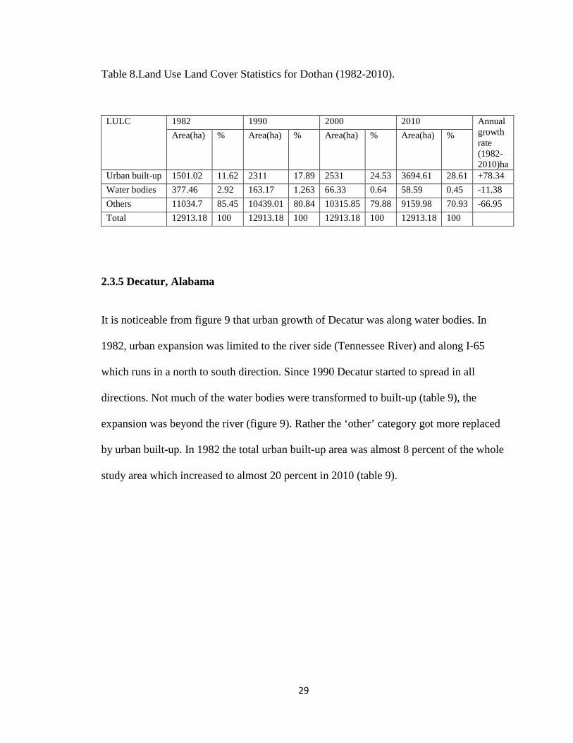
Table 8.Land Use Land Cover Statistics for Dothan (1982-2010).

2.3.5 Decatur, Alabama

It is noticeable from figure 9 that urban growth of Decatur was along water bodies. In

1982, urban expansion was limited to the river side (Tennessee River) and along I-65

which runs in a north to south direction. Since 1990 Decatur started to spread in all

directions. Not much of the water bodies were transformed to built-up (table 9), the

expansion was beyond the river (figure 9). Rather the ‘other’ category got more replaced

by urban built-up. In 1982 the total urban built-up area was almost 8 percent of the whole

study area which increased to almost 20 percent in 2010 (table 9).



Urban built-up 1501.02 11.62 2311 17.89 2531 24.53 3694.61 28.61 +78.34 Water bodies 377.46 2.92 163.17 1.263 66.33 0.64 58.59 0.45 -11.38 Others 11034.7 85.45 10439.01 80.84 10315.85 79.88 9159.98 70.93 -66.95 Total 12913.18 100 12913.18 100 12913.18 100 12913.18 100

30

Figure 9. Urban Built-up Expansion for Decatur.

Table 8.Land Use Land Cover Statistics for Decatur (1982-2010).



Urban built-up 1729.98 7.80 3102.12 17.02 3205.66 17.59 3519.57 19.31 +63.91 Water bodies 3165.57 17.37 2597.83 14.25 2305.11 12.65 2132.02 11.70 -36.91 Others 13326.2 73.13 12521.8 68.71 12710.98 69.7 12570.16 68.98 -26.99 Total 18221.75 100 18221.75 100 18221.75 100 18221.75 100

31

2.3.6 Huntsville and Madison, Alabama

Spatial expansion of urban or built-up areas of Huntsville is distinctly shown in figure 10.

In 1982, the urban built-up area occupied only 3.15 percent of the total land area for

Huntsville and was mainly located along the interstate 565 corridor. Significant urban

expansion was shown to have taken place in 1990, 2000, and 2010, with net addition of

4578, 520, and 603.6 hectares, respectively. The outward expansion of built-up areas

(table 10) in these three decades tends to follow major transportation routes and is highly

concentrated in central and western part of the study area (figure 10 left).

Figure 10.Urban Built-up Expansion for Huntsville (left) and Madison (right).

32

Table 9. Land Use Land Cover Statistics for Huntsville (1982-2010).

For Madison, in 1982 urban built-up areas were mainly concentrated near I-565.

From 1990, it started to spread towards north. In 2010, it dispersed all over the study area

(figure 10 right). Population grew over 900 percent from 1980 to 2010. Net addition of

urban built-up area is 2551.81 hectares (over 600 percent).

Table 10. Land Use Land Cover Statistics for Madison (1982-2010).

2.3.7 Auburn, Alabama

Based on figure 11, urban built-up expansion for Auburn mainly follows north-east to

south-west direction. From 1982 to 2010, it has taken place both side of I-85. Urban

expansion mainly concentrated in the central place of study area (due to presence of

urban functions, such as schools) and expansion was more southern part than the northern

part (figure 11).



Urban built-up 2462.67 3.15 7040.79 9.1 7561.37 9.68 8165 10.5 +203.6 Water bodies 489 0.62 461 0.6 407.5 0.52 386 0.5 -3.7 Others 75124.5 96.21 70574.3 90.3 70107.3 89.8 69525.2 89.0 199.97 Total 78076.17 100 78076.17 100 78076.17 100 78076.17 100



Urban built-

376.85 3.88 1000.8 10.31 2283.86 23.54

2928.66 30.19

+91.13 Water b di

84.25 0.86 65.43 0.75 32.38 0.33 25.32 0.26

-2.10 Others 9237.12 95.24 8631.9 89.0 7381.98 76.1

1 6744.24 69.

54 -89.03

Total 9698.22 100 9698.22 100 9698.22 100 9698.22 100

33

In 1982, total urban built-up area was approximately 5.4 percent and in 2010, it

was 33.7 percent (table 12). So the net addition was over 600 percent.

Figure 11. Urban Built-up Expansion for Auburn.

Table 11. Land Use Land Cover Statistics for Auburn (1982-2010).



Urban built-up 423.18 5.36 1084.59 13.76 1288.8 16.35 1985.31 33.78 +55.79 Water bodies 64.35 0.81 35.4 0.523 30.6 0.388 19.71 0.33 -1.59 Others 7394.31 93.81 6761.85 85.79 6562.44 83.26 5876.82 74.56 54.19 Total 7881.84 100 7881.84 100 7881.84 100 7881.84 100

34

2.3.8 Tuscaloosa, Alabama

Based on figure 12, the nature of change is quite clear. Spatial expansion of urban built-

up area was mainly determined by the presence of large water body (Black Warrior

River). Most of the expansion took south of the water body. It did not follow any

significant transportation route. From 1982 to 2010, water bodies decreased gradually

although built-up did not increase significantly. The net addition was 30 percent for

Tuscaloosa urban area (table 13).

Figure 12. Urban Built-up Expansion for Tuscaloosa.

35

Table 12. Land Use Land Cover Statistics for Tuscaloosa (1982-2010).



Urban built-up 3222.36 15.17 3308.4 15.57 3712 17.47 4210 19.88 +35.27 Water bodies 653.94 3.07 617.4 2.90 401 1.88 256.23 1.20 -14.20 Others 17361.9 81.74 17312.4 81.51 17125.2 80.63 16771.97 78.97 21.06 Total 21238.2 100 21238.2 100 21238.2 100 21238.2 100

2.4 Accuracy Assessment of Classified Images

Because of the limited availability of ground reference data, it was impossible to perform

accuracy assessment for all images with authenticity. The strategy which is adopted here

to assess the accuracy is to calculate using stratified random sampling method and Kappa

statistics were also computed.

The supervised classification of each image consisted of three classes. Using the

stratified random sampling a total of 50 random points were created for each image. Once

the points were created for each image, the accuracy assessment was initiated. Because of

the limited availability of ground reference data, the accuracy of these images is limited.

The minimum accuracy was 75 percent and the maximum accuracy was more than 80

percent (table 14).

Various literatures (Yang 2002, Matlab et al 2005, Trousdale 2010) mentioned

that the ‘other’ land cover type caused most of the error because it contains different

types of land use (table 3).

36

Table 13. Accuracy Assessment and Kappa Statistics of Classified Image.

Urban Built-up Area Accuracy Assessment (%) Kappa Statistics 1982 1990 2000 2010 1982 1990 2000 2010

Auburn 76.1 75.3 79.1 78.0 .755 .744 .789 .779 Dothan 75.3 77.8 78.5 77.2 .745 .767 .788 .771 Tuscaloosa 77.4 77.3 75.7 75.4 .777 .756 .749 .749 Mobile 77.2 80.1 75.6 75.4 .773 .799 .766 .755 Huntsville 75.2 78.1 76.2 76.7 .765 .773 .766 .766 Decatur 79.7 75.3 76.1 77.2 .779 .742 .763 .777 Birmingham 77.5 75.1 75.2 77.9 .789 .755 .746 .771 Montgomery 79.7 76.2 78.2 78.1 .799 .771 .779 .779

2.5 Summary

In conclusion, supervised classification technique applied to quantify urban expansion in

the ten study areas. Figure 13 represents graphical representation of urban built-up area

expansion from 1982 to 2010.Graph is very steep for Auburn and Madison whereas

Tuscaloosa, Birmingham grew very gradually.

Figure 13. Urban Built-up Area Statistics (1982-2010)

Different urban areas showed varied spatial patterns of growth due to influential

factors like presence of transportation routes and water bodies. Literatures also found to

37

support this statement (Li et al 2003, Meng et al 2003,Peng et al 2006, Yang 2002).

Birmingham, Montgomery, Dothan, Huntsville, Madison and Auburn showed significant

patterns of growth around transportation routes such as interstate highways and state

highways. This expansion can be attributed to economic activities that highways attract.

On other hand, water bodies dominated the growth of urban areas like Mobile, Decatur

and Tuscaloosa.

38

Chapter 3: Urbanization and Impact on Environment

3.1 Introduction

Previous research has highlighted how different environmental parameters (temperature,

precipitation, and air quality: ozone and PM 2.5) are changing with time over urban areas

and their correlation with built up expansion globally (Tayanc and Toros 1997, Mitra et

al 2011, Superczynski and Christopher 2011, Babatola 2013). Temperature and

precipitation are fundamental components of environment and changes in their pattern

can affect human health, ecosystems, plants, and animals. These two variables are also

interconnected. An increase in Earth’s temperature leads to more evaporation and cloud

formation, which in turn, increases precipitation (Tabari et al 2013). So it is important to

understand and quantify the variability or anomaly in these weather elements over time

especially for urban areas where change is very rapid.

This chapter focuses on trend detection in annual temperature, precipitation and

air quality (O3 and PM 2.5) of all study areas from 1980 to 2010 using Mann-Kendall

(MK) trend test and examines whether urban built-up expansion has an impact on

environmental parameters using multiple linear regression.

39

3.2 Temporal Trends of Environmental Parameters

The temporal trends of some random variables exhibit a trend such that there is a

significant change (negative or positive) over time. Statistical procedures are used for the

detection of the gradual trends over time (Bayazit and Onoz 2003). The purpose of trend

testing is to determine whether the values of a random variable generally increase or

decrease over some period of time in statistical terms (Helsel and Hirch 1992; Bayazit

and Onoz 2003).

Trend analysis is an active area of interest in climatology, hydrology, water

quality, and other natural sciences for over three decades (Mustapha 2013). Detection of

temporal trends is very important to monitor environmental parameters because these

kinds of data are often carried out to assess the human impacts on the environment

(Libiseller and Grimvall 2002) and also because some projects mainly based on historical

pattern of environmental behaviors (Mustapha 2013).

Non parametric trend tests require data which are independent and can tolerate

outliers in data (Onoz and Bayazit 2003). There are many non- parametric trend tests use

to analyze the temporal trends. The Mann Kendall (MK) test (Mann 1945; Kendall 1955;

Mitra et al 2011) is one of the widely used non-parametric tests to detect the significant

trends in the time series (Hameed 2008, Mustapha 2013). MK test to detect trend in

environmental data (temperature, precipitation, and air quality) have been used by many

scholars (Gilbert 1987, Serrano et al 1999, Yue et al 2002, Libiseller and Grimvall 2002,

Kahya and kalayci 2004, Hameed 2008, Buhairi 2010, Mitra et al 2011, Mustapha 2013,

and Lunge and Deshmukh 2013).

40

Yue et al (2002) documented the power of two trend tests (Mann–Kendall test

and Spearman's rho test) in their paper. According to them, power of trend tests depends

on the pre-assigned significance level, magnitude of trend, sample size, and the amount

of variation within a time series meaning the bigger the absolute magnitude of trend the

more powerful are the tests. With a large sample size, the tests become more powerful

and as the amount of variation increases within a time series, the power of the tests

decrease (Yue et al 2002). Another study by Kahya and Kalayci (2004) examined four

non-parametric trend tests (the Sen's T, the Spearman's Rho, the Mann-Kendall, and the

Seasonal Kendall) to understand the trend analysis of stream flow in Turkey. In order to

detect possible trends in precipitation over the Iberian Peninsula, the Mann-Kendall test

was applied to the annual and monthly series (Serrano et al 1999).

In this study, Mann-Kendal test was performed to understand the temporal trends

of environmental parameters (temperature, precipitation, ozone, and particulate matter

2.5) for ten study areas from 1980 to 2010 which are non-parametric. Here observations

were made annually from one single station for each study area.

3.3 Relationship between Environmental Parameters and Urban Built-up Area

A study by Mitra et al (2011) suggests that there is a positive relationship between

growth of a city and rainfall amount. Particularly the findings of their study indicated that

urban land cover change has had a positive effect in increasing pre-monsoon rainfall in

Kolkata, India. Babatola (2013) also found in his study that urbanization increases

relative-humidity and that relative humidity has corresponding influence on rainfall in

Ibadan, Nigeria. Another study in Turkey reveals that four urban measurement stations

41

and their neighboring rural sites for the 1951-1990 time periods have experienced a shift

towards the warmer side with respect to the frequency distributions of daily minimum

temperature (Tayanc and Toros 1997).

Kalnay & Cai (2003) estimated the impact of urbanization and other land uses on

climate change by comparing trends observed by surface stations with surface

temperatures over a 50 year period. Their results indicate that half of the observed

stations experienced a decrease in diurnal temperature range due to urban and other land-

use changes.

Studies that attempt to relate air pollution and urban growth are limited in number

(Superczynski and Christopher 2011). Weng et al (2006) however, investigated the

relationship between pollutant particles (SO2, NOx, dust) and urban infrastructure in

China. They used Geographic Information System (GIS) as a technique to correlate urban

concentration and pollution. They found that pollution levels were significantly

correlated to the regions around the pollution centers. Another study also found

connection between pollutant material (PM2.5) and LULC in Birmingham, AL

(Superczynski and Christopher 2011). In this study the researchers used GIS and remote

sensing techniques to determine the relationship between PM2.5 and urban area in 1998

and 2010 and they found moderate to strong impact.

In this research, relationship between urban built up expansion and environmental

parameters has been established through multiple linear regression analysis (Appendix

B). This model also provides a module of ANOVA that gives the information whether

model itself is statistically significant or not (Sundari et al 2013). Many scholars used

42

regression in urban environment study (Fushimi et al 2005, Denby 2008, Manquiz et al

2010, Sundari et al 2013, Mekparyup 2013, and Hug et al 2013) and their results support

the reliability of the model.

3.4 Data and Data Sources

The data for this study were collected from different sources from 1980 to 2010.

Temperature and precipitation data were collected mainly from National Weather Service

(NWS), National Climatic Data Center (NCDC), and Environmental Protection Agency

(EPA) (Appendix A). The datasets were not normally distributed though they are

randomly distributed.

3.5 Methodology

3.5.1 MK Trend Test

There are two advantages of using the MK test. First it does not require the data to be

normally distributed (distribution of normal variables as a symmetrical bell shaped

curve). Second it is less affected by outliers because its statistic is based on the sign

differences, not directly on the values of the random variables (Kahya and kalayci 2004,

Tabari et al 2011). According to this test, the null hypothesis H0 assumes that there is no

trend (the data is independent and randomly ordered) and this is tested against the

alternative hypothesis H1, which assumes that there is a trend (Onoz and Bayazit 2003).

The basic principle of MK test is based on statistics (S). MK (S) statistic is

computed as follows:

43

𝑆 = ∑ ∑ 𝑠𝑖𝑔𝑛(𝑥𝑗𝑛𝑗=𝑘+1 − 𝑥𝑘𝑛−1

𝑘=1 )

S= Mk test value

Xj and Xk = Sequential data values

K and n = length of data

S value is assumed to be 0 (no trend). A very high positive value of S indicates an

increasing trend and a very low negative value indicates a decreasing trend.

The MK test also computes Kendall’s Tau nonparametric correlation coefficient.

It measures the strength of relationship between two variables (Gilbert 1987). The value

ranges from +1 to -1. Positive correlation indicates both of the variables increase together

whereas negative correlation indicates that if one variable increases; the other decreases

(Gilbert 1987).

Software used for performing the statistical Mann-Kendall test is Addinsoft’s

XLSTAT 2013 (figure 14). On running the Mann-Kendall test on environmental

parameter data, if the p value is less than the significance level α (alpha) = 0.05, H0 is

rejected. Rejecting H0 (accept H1) indicates that there is a trend in the time series, while

accepting H0 indicates no trend was detected. On rejecting the null hypothesis, the result

is said to be statistically significant.

44

Figure 14. Screen Shot of MK test in Addinsoft’s XLSTAT 2013.

In this study, it is hypothesized that all the environmental parameters should has

an increasing trend with time.

3.5.2 Multiple Linear Regression

In statistics, linear regression is an approach to modeling the relationship between a

dependent variable and one or more explanatory variables. The case of one explanatory

variable is called simple linear regression. For more than one independent variable, it is

called multiple linear regressions (Jolliffe 1982).

In a simple linear regression model, a single response measurement Y is related to

a single predictor X for each observation. Here the critical assumption of the model is

that the conditional mean function is linear: E(Y |X) = α + βX. In most problems, more

than one predictor variable will be available.

For this research, the equation should be:

Y = α +β1X1+ β 2X 2+ β 3X 3

Y= Temperature, precipitation, ozone and PM 2.5

X1=Urban built-up

X2=Water

45

X3=Other

There should be a linear relationship between independent and dependent

variables (Denby 2008, Manquiz et al 2010, Sundari et al 2013). It means if the

dependent variable increases, independent variable will increase too. For instance, in this

study if urban built-up area increases temperature will also increase.

Table 14 : Variables and their Indicators

Results can be explained by R square value, P value and coefficient value. R

square value indicates how much of the variation in the dependent variable can be

explained by variations in the three independent variables. If the F significance value is

less than 0.05, the regression equation is effective as a whole. If p value is less than 0.05

for a variable, it has an impact on dependent variable. Coefficient value indicates how the

variables are correlated: positively or negatively.

Classes Variables Indicators Assumptions Dependent Variables

Temperature Average temperature in year (⁰F)

Urban built-up area is expected to positively relate to temperature, precipitation, PM 2.5 and Ozone. Water bodies and other LULC are expected to negatively relate to temperature, precipitation, PM 2.5 and Ozone.

Precipitation Average precipitation in year (inch)

PM 2.5 Annual concentration in air (µg/m 3)

Ozone Annual concentration in air (ppm)

Independent Variables

Urban built- up Size in hectors Water bodies Size in hectors

Other Size in hectors

46

This model has been run four times for four dependent variables. The reason for

choosing the four environmental parameters as dependent variables is because they can

vary with changing LULC. The model was obtained by data analysis using Microsoft

excel (figure 15).

Figure 15. Multiple Linear Regression in Excel.

3.6 Results

3.6.1 Trend Analysis using MK Trend Test

Man-Kendall test was applied to the environmental parameters data (temperature,

precipitation, ozone, and PM2.5) to verify the increasing or decreasing trends for 1980 to

2010. In this study X variable is time and Y variables are environmental parameters

(figure 16).

47

Figure 16. Temporal Trends for Madison, Alabama (1980-2010).

Temperature

On running the MK test on temperature data, the following results in Table 16 were

obtained for ten study areas.

The Mann-Kendall test confirmed that the positive trend observed in temperature

data is statistically significant (p values are less than 0.05). S values are also positive and

much higher than 1, it indicates an increasing trend in temperature data for every study

area. Kendall’s tau values are also positive; it proves that temperature has increased from

1980 to 2010.

48

Table 15. Mann-Kendall Summary of Temperature Data for the Ten Study Areas (1980-2010).

Study Area Results of MK trend test for temperature

Mann-

Kendall

Statistics

(S)

Kendall’s

Tau

P value alpha Test

interpretation

Trend

Birmingham 40 0.354 .0045 0.05 Reject H0 ↑ Increasing

Montgomery 43 0.222 .0013 0.05 Reject H0 ↑ Increasing

Mobile 31 0.256 .0002 0.05 Reject H0 ↑ Increasing

Huntsville 33 0.344 .0001 0.05 Reject H0 ↑ Increasing

Tuscaloosa 48 0.211 .0004 0.05 Reject H0 ↑ Increasing

Hoover 40 0.354 .0045 0.05 Reject H0 ↑ Increasing

Dothan 52 0.347 .0015 0.05 Reject H0 ↑ Increasing

Decatur 22 0.214 .0001 0.05 Reject H0 ↑ Increasing

Auburn 28 0.365 .0001 0.05 Reject H0 ↑ Increasing

Madison 33 0.344 .0001 0.05 Reject H0 ↑ Increasing

This increased trend in temperature is attributed to concrete surface and

greenhouse gas emission (Han et al 2013 and Buhairi 2010). Various urban heat island

studies revealed that temperature in the urban are is higher than its surround rural area

(Garstang 1975, Morris and Simmonds 2000).

49

Precipitation

For precipitation (1980-2010) data in ten study areas shows an increasing trend (table

17). Here p values are less than 0.05 for every study area. Thus null hypotheses are

rejected. On rejecting the null hypothesis, the result is said to be statistically significant.

Kendall’s tau and S values also (both values are positive) revealed a positive trend in data

set.

Under thermodynamic conditions that are conducive to moist convection, the

urban heat island-induced updrafts act as dynamic forcing to initiate moist convection

and produce surface precipitation. Surface precipitation is likely to further increase under

higher aerosol concentrations if the air humidity is high and deep and strong convection

occurs (Han et al 2013, Babatola 2013).

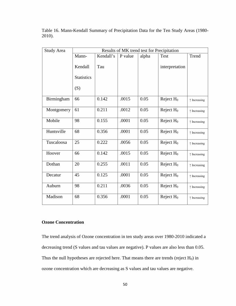
50

Table 16. Mann-Kendall Summary of Precipitation Data for the Ten Study Areas (1980-2010).

Study Area Results of MK trend test for Precipitation

Mann-

Kendall

Statistics

(S)

Kendall’s

Tau

P value alpha Test

interpretation

Trend

Birmingham 66 0.142 .0015 0.05 Reject H0 ↑ Increasing

Montgomery 61 0.211 .0012 0.05 Reject H0 ↑ Increasing

Mobile 98 0.155 .0001 0.05 Reject H0 ↑ Increasing

Huntsville 68 0.356 .0001 0.05 Reject H0 ↑ Increasing

Tuscaloosa 25 0.222 .0056 0.05 Reject H0 ↑ Increasing

Hoover 66 0.142 .0015 0.05 Reject H0 ↑ Increasing

Dothan 20 0.255 .0011 0.05 Reject H0 ↑ Increasing

Decatur 45 0.125 .0001 0.05 Reject H0 ↑ Increasing

Auburn 98 0.211 .0036 0.05 Reject H0 ↑ Increasing

Madison 68 0.356 .0001 0.05 Reject H0 ↑ Increasing

Ozone Concentration

The trend analysis of Ozone concentration in ten study areas over 1980-2010 indicated a

decreasing trend (S values and tau values are negative). P values are also less than 0.05.

Thus the null hypotheses are rejected here. That means there are trends (reject H0) in

ozone concentration which are decreasing as S values and tau values are negative.

51

Table 17. Mann-Kendall Summary of Ozone Data for the Ten Study Areas (1980-2010).

Particulate Matter 2.5 (PM2.5)

This following table represents the results of PM2.5 concentration in air for ten study areas

(1980-2010). Here P values are less than 0.05. It indicates the result is statistically

significant. S values (negative) and tau values (negative) also proved that PM2.5 has a

decreasing trend in 30 years in all the study areas.

Study Area Results of MK trend test for Ozone

Mann-

Kendall

Statistics

(S)

Kendall’s

Tau

P value alpha Test

interpretation

Trend

Birmingham -58 -0.211 0.008 0.05 Reject H0 ↓ Decreasing

Montgomery -44 -0.104 0.035 0.05 Reject H0 ↓ Decreasing

Mobile -65 -0.233 0.018 0.05 Reject H0 ↓ Decreasing

Huntsville -61 -0.365 0.002 0.05 Reject H0 ↓ Decreasing

Tuscaloosa -48 -0.296 0.044 0.05 Reject H0 ↓ Decreasing

Hoover -58 -0.211 0.033 0.05 Reject H0 ↓ Decreasing

Dothan -22 -0.122 0.030 0.05 Reject H0 ↓ Decreasing

Decatur -47 -0.452 0.027 0.05 Reject H0 ↓ Decreasing

Auburn -22 -0.366 0.032 0.05 Reject H0 ↓ Decreasing

Madison -61 -0.365 0.019 0.05 Reject H0 ↓ Decreasing

52

Table 18. Mann-Kendall Summary of PM2.5 Data for the Ten Study Areas (1980-2010).

Study Area Results of MK trend test for PM 2.5

Mann-

Kendall

Statistics

(S)

Kendall’s

Tau

P value alpha Test

interpretation

Trend

Birmingham -36 -0.320 0.025 0.05 Reject H0 ↓ Decreasing

Montgomery -47 -0.213 0.029 0.05 Reject H0 ↓ Decreasing

Mobile -27 -0.278 0.019 0.05 Reject H0 ↓ Decreasing

Huntsville -51 -0.388 0.043 0.05 Reject H0 ↓ Decreasing

Tuscaloosa -33 -0.359 0.045 0.05 Reject H0 ↓ Decreasing

Hoover -36 -0.320 0.036 0.05 Reject H0 ↓ Decreasing

Dothan -39 -0.345 0.005 0.05 Reject H0 ↓ Decreasing

Decatur -88 -0.356 0.029 0.05 Reject H0 ↓ Decreasing

Auburn -47 -0.334 0.027 0.05 Reject H0 ↓ Decreasing

Madison -51 -0.388 0.033 0.05 Reject H0 ↓ Decreasing

3.6.2 Multiple Linear Regressions

Model 1: Temperature as Dependent Variable

A multiple regression was conducted to understand how temperature can vary with

different land use land cover. The overall model was significant (F value is less than .05)

and accounted for the 72.36 percent of the variance (table 20). That means 72.3 percent

of the variation in the temperature explained by urban built-up, water and other LULC.

53

The results indicated that urban built-up, and other LULC were significant

variables of the temperature variation (p value is less than 0.05). Water bodies were not

significant variable (p value is more than 0.05) (table 20).

At the significant level of 0.05, positive and small coefficient of urban built-up

indicates that higher urban built-up area is associated with higher temperature (table 20).

Table 19. Regression Results for Temperature.

Variables Coefficients P-value Intercept 64.1501642 3.17744E-47 Urban Built-up 0.000180636 0.032674734 Water body -0.000228902 0.429368727 Other -2.87942E-05 0.005284124 R Square Value 0.723632792 F Significance 0.026322768

Model 2: Precipitation as Dependent Variable

From the ANOVA table (table 21), F significance is less than 0.05. The mode is highly

significant. The R square value means that 65.94 percent of the variation in precipitation

can be attributed to three independent variables (table 21). This is not a very high

percentage as roughly 34 percent is left unexplained.

Regression results also revealed that urban built-up is a significant variable to

determine the amount of precipitation. Positive coefficient value and P value support this

statement (table 21).

54

Rest of the variables (water bodies and other) was also significant. However other

category is negatively correlated with precipitation whereas water bodies are positively

correlated (table 21).

Table 20. Regression Results for Precipitation.

Model 3: Ozone as Dependent Variable

The F value (more than 0.05) of the model indicates that this model is not significant

(0.200075634). Thus independent variables are not significant for ozone concentration in

air at all.

Model 4: PM2.5 as Dependent Variable

For this regression model, R square value is a very high. 86.2 percent of the variation in

PM 2.5 concentration can be explained by three independent variables (table 21 a). F value

(less than 0.05) from ANOVA table also proved the effectiveness of this model (table 22)

Positive coefficient and P value (0.004) of urban built-up also suggest that if

urban built-up area goes high, the concentration of PM2.5 in air also goes high (table 22).

‘Other’ variable have negative effect on PM2.5 (table 22). However water body was not

significant for PM 2.5 since p value is more than 0.05 thought it has negative coefficient

value (table 22).

Variables Coefficients P-value Intercept 54.48773419 6.38519E-34 Urban Built-up 0.000253938 0.027448967 Water body 0.001500062 0.012901341 Other -4.12031E-05 0.040740165 R Square Value 0.659446819 F Significance 0.011957406

55

Table 21. Regression Results for PM 2.5.

The main reason for the improved air quality in Alabama is the ‘Revisions to the

Clean Air Act’ in 1990 required each state to develop a State Implementation Plan (SIP)

describing how it will reach and maintain the national standards (EPA 2012a). These

SIPs vary by state, but generally include local monitoring of air quality levels, strategies

to reduce emissions, and steps to evaluate these strategies. Individual actions that can also

make a difference include recycling, using energy-efficient products and appliances,

planting deciduous trees, and driving less.

3.7 Summary

This chapter briefly analyzed temporal trends of environmental parameters and how they

vary with urban built-up expansion. A gradual increase in temperature and precipitation

and a decrease in ozone and PM2.5 were observed for study areas over a period of 1980 to

2010.

Results of multiple linear regression revealed that variation in temperature,

precipitation and PM2.5 can be explained by urban built-up expansion. So the results

fulfill the assumptions that there is a cause and effect relationship between urban built-up

expansion and environmental parameters. However, variation in ozone cannot be

explained by urban built-up expansion (F value was not significant).

Variables Coefficients P-value Intercept 18.5005228 2.30993E-22 Urban Built-up 0.000363319 0.004234144 Water body -0.000458622 0.283836639 Other -7.94683E-05 2.37939E-06 R Square Value 0.861704408 F Significance 1.33E-06

56

Chapter 4: A Peek into Future Urban Growth

4.1 Introduction

Predictions say that urban population will rise to 70 – 80 percent globally of the total

population (UN 2007). Thus it would be interesting to see how present urban areas will

look like in next 30 – 40 years. To run these futuristic predictions it is important to use

reliable LULCC models. These models can predict the spatial distribution of the specific

LULC classes for future years by utilizing the knowledge gained from previous years

(Behera et al 2012). LULC models are different from each other and have their own

capabilities and limitations (Chen and Pontius 2006). There are various land use change

models: DELTA, Land change modeler, What If, SLEUTH, LTM, Markov model and

others (EPA 2000). Cellular Automata Markov chain is one of the accepted methods for

modeling LULCC (Mitsova et al 2011; Kityuttachai et al 2013).

In this study the IDRISI CA (Cellular Automata) – Markov model has been used

to predict the future growth of the Alabama urban areas. CA-Markov method has two

techniques: Markov chain analysis and CA. The spatial character in a model is introduced

by CA component. It allows the transition probabilities of one pixel to be a function of

the neighboring pixels. CA-Markov models the change of several classes of cells by

using a Markov transition matrix; a suitability map and a neighborhood filter (Eastman

2000).

57

The IDRISI Selva, an integrated GIS and Image Processing software, has a built-

in CA Markov model that can be used to project the future growth of urban built-up areas

of the State of Alabama. The literature has shown that CA Markov models have been

successful in predicting future growth of urban areas. Araya and Cabral (2010), Guan et

al (2011) Behera et al (2012), and Kityuttachai et al (2013) used the CA Markov model

to predict future urban growth of various global cities and highly recommend the use of

the model.

4.2 Future Urban Growth using CA Markov Model

Future growth of five urban built-up areas has been predicted using cellular automata

IDRISI Selva model for the next 30 years from 2010 based on the results from the

supervised classification shown in chapter 2: three of which showed highest growth in

population (Madison, Hoover and Auburn) and two which showed decrease in population

in 30 years (Birmingham and Mobile) from 1982 to 2010. The two classified (1982 and

2010) Landsat images derived from objective 1 and accuracy assessment of the

classifications both were required to run the model (Behera et al 2012). To predict the

future growth, it is important to know the extent of built-up area and

vegetation/agricultural land on which development can occur and water on which

development cannot occur.

To run the model, the images should be: (1) derived from grids in the same

projection, (2) derived from grids of the same map extent, (3) verified to be of the same

resolution (row x column count is consistent), and (4) verified to be of the same class

value. The next step was to import the images into IDRISI Selva and convert them to

58

*.rst images because it does not accept *.img images. Then, a Markov chain analysis was

run on both images. The output from the Markov chain analysis was used to initialize the

CA – Markov analysis (Guan et al 2011). The images run through a series of tasks to get

the projection of the urban built-up areas in Alabama up to 2040. Classified images from

objective one was used here to predict future urban expansion. Figure 17 displays a flow

diagram of the CA-Markov modeling process.

4.2.1 Cross Classification of Two Images

Cross classification is a common application in land cover change analysis where a cross

tabulation is done between two qualitative maps of two different dates that targets on the

same features (IDRISI 2012). It is used to compare two classified images where the

classification assigns the same unique and distinct identifier to each class on both the

dates. The aim is to evaluate whether the areas fall into the same class on the two dates or

a change to a new class has occurred (IDRISI 2012). By running a CROSSTAB module

in IDRISI SELVA it is possible to get a new image based on all the unique combination

of values from the two images in which each unique combination of input values has a

unique output value and a cross tabulation table.

Cross correlation images show all possible combinations that are used to produce

two types of change images. These relative frequencies are known as transition

probabilities and are an underlying basis for Markov Chain prediction of future

transitions (Mitsova et al 2011; IDRISI 2012).

In this study cross classification was run between classified images of 1982 and

2010 for five study areas.

59

Figure 17. Flow diagram showing this study’s CA-Markov Model Design.

4.2.2 Markov Chain Analysis

The Markov chain analysis describes the probability of land cover change from one

60

period to another by developing a transition probability matrix (Eastman 2000). The

output of this step are a transition probability matrix, a transition area matrix and a set of

transition probability maps by analyzing two qualitative land use images (Islam and

Ahmed 2011). The transition probability matrix records the probability of each land use

category to change into the other category. This matrix is produced by the multiplication

of each column in the transition probability matrix be the number of cells of

corresponding land use in the later image (Islam and Ahmed 2011). The transition areas

matrix is a text file that records the number of pixels that are expected to change from

each land cover type to the other land cover type over the specified number of time units

(Adhikari and Southworth 2012). It will be used as an input to run CA-Markov model.

Transition probability maps were created for every category of LULC.

The Markov chain analysis though one of the best has its limitations. Markov

analysis does not account the causes of land use change. It ignores the forces and

processes that produced the observed patterns (Adhikari and Southworth 2012). It

assumes that the forces that produced the changes will continue to do so in the future. An

even more serious problem of Markov analysis is that it is insensitive to space: it

provides no sense of geography (Mubea et al 2010, Adhikari and Southworth 2012).

Using cellular automata adds a spatial dimension to the model (Mubea et al 2010).

4.2.3 Cellular Automata (CA)

Cellular automata (CA) are spatially dynamic models frequently used for land-use and

land-cover change studies (Mitsova et al 2011). In a CA model, the transition of a cell

from one land-cover to another depends on the state of the neighborhood cells. A CA

61

model can add spatial character to a Markov model and make it a dynamic spatial model

(Mubea et al 2010, IDRISI 2012).

4.2.4 CA Markov Model

A combined Markov and CA model was used to predict the future LULC of the five

urban areas of Alabama. Transition area matrix (output of Markov model) was used here.

In addition, to get the suitable image collection, multi-criteria evaluation (MCE) has been

run. MCE is a common method for assessing and aggregating many criteria (IDRISI

2012). Two types of criteria (constraints and factors) were developed to determine which

lands were more suitable for future development or not. The constraints were

standardized into a Boolean character of 0 and 1 and the factors were standardized to

continuous scale of 0 (least suitable) to 255 (more suitable). Here the constraints were

water bodies and existing urban areas. Factors were presence of water bodies, road

network, slope and elevation. Three types of fuzzy membership functions were used to

rescale the factors into the range 0-255: sigmoidal, linear and symmetrical. Analytic

hierarchy process (AHP) was used to determine the weight of factors (Mitsova et al

2011).

The CA-Markov model is based on the first law of geography by using a

contiguity rule. That means, a pixel that is near one specific LULC is more likely to

become that category than a pixel that farther (Araya and Cabral 2010). Here, a contiguity

filter of 5*5 pixels was applied.

62

4.2.5 Model Validation

Model validation is very important step in the modelling process (Araya and Cabral

2010). The location accuracy of land use change was done on Neural Network built-in

module in the IDRISI (IDRISI 2012). The input for this method was 2010 and 2040

image. This method was able to provide the accuracy of future location compare to recent

location on the basis of constraints (water body and existing urban built-up area) and

factors (presence of water bodies, road network, slope and elevation).

In this study, another accuracy assessment was also performed on the 2013 CA-

Markov output image and the Google earth image to understand how accurate the

prediction is for 2040. 65 random points were used for each study area to perform the

accuracy assessment. In this case only 50 could be plotted as the other points were

outside of the image. A visual assessment of the points on both the images were done and

compared with the help of the classification error matrix.

4.3 Results

4.3.1Transition Probability Matrix

The Markov model calculates transition probabilities (table 23) as a txt file with the

number of transitioning cells from one LULC to another. Another output is raster grids,

indicating transition areas (Mitsova et al 2011). The later one was used for CA-Markov

model. Markov transition probability matrix is computed from cross classification of two

classified images (1982 and 2010). Transition areas are derived by multiplying each

column representing LULC in probability matrix (Mitsova et al 2011).

63

The transition probability matrices of LULC for Madison, Hoover, Auburn,

Birmingham, and Mobile for 1982-2010 calculated on the basis of the Markov model are

shown in table 23. The diagonal cross section of each study area (shown in bold in table

23) represents the probability of a LULC remaining the same whereas the off diagonal

values (not in bold) indicate the probability of a change occurring from one LULC to

another (table 23).

Table 22. Transition Probability Matrix of Markov Model for Five Study Areas.

From the table 23 it is evident that most of the LULC remained same except the

‘other’ category. The transition rules allowed water pixels to remain almost unchanged.

Study Area Given (1982-2010) Probability of changing to -

Class 1: Water

Class 2: Other

Class 3: Urban built-up

Madison Class 1: Water 0.9989 0.001 0.0001

Class 2: Other 0.0005 0.7452 0.2543 Class 3: Urban built-up 0.0006 0.012 0.9472

Hoover Class 1: Water 0.4053 0.3072 0.2075


Auburn Class 1: Water 0.7870 0.1066 0.1064


Birmingham Class 1: Water 0.8833 0.0545 0.0622


Mobile Class 1: Water 0.9045 0.0007 0.0948


64

Other LULC was converted mostly to urban built-up area but the rate varied with every

study area. May be the reason was ‘other’ category includes vacant land and various

types of vegetation which is more vulnerable to convert. Urban built-up area remained

unchanged since it is very rare to convert built-up area to vegetation or water body.

Table 23 indicates that during 1982-2010 there was 25.4 percent chance that

‘other’ category would transform to urban built area for Madison. Percentage was highest

for Hoover (42.5 percent) and lowest for Mobile (17.3 percent). The rate was 39.5 and

32.7 percent for Auburn and Birmingham respectively. On the other hand, water bodies

transformed to urban built-up area (10 and 6 percent for Auburn and Birmingham

respectively) and ‘other’ (30 percent for Hoover) in a very low rate. The rate of

transformation for urban built-up area to water body and ‘other’ was also very low (0

percent and 17 percent respectively of for Auburn).

As a result urban built-up increased continuously and ‘other’ category decreased.

Water body remained unchanged. The increasing source for conversion to urban area

was ‘other’ category.

4.3.2 Urban Built-Up Area Prediction for the year 2040

After running cross classification and Markov model, it was interesting to examine the

pattern and tendency of the change of built-up area for the future. Prediction for the 2040

was carried out for five selected study areas considering transition area matrix, a

contiguity filter and the transition suitability collection.

Here the two constraints were water bodies and existing urban built-up area. It

means that future urban could not take in these two specified place. The factors were

65

slopes, elevation, roads, and distance for water body of the study areas. These factors

determine the quantity and location of future change of LULC (Guan et al 2011). The

sum of the factors should be 1 (IDRISI 2012). Smaller weight is less effective to

determine the predicted LULC compare to higher weight. It means, roads and water

bodies were more effective than other two (table 24).

Table 23. Factors Controlling Future Growth (derived from MCE).

Study Area Factors Weight Madison

Slope 0.16 Elevation 0.20 Roads 0.31 Water bodies 0.33

Hoover


Auburn


Birmingham Slope 0.10 Elevation 0.25 Roads 0.26 Water bodies 0.39

Mobile Slope 0.21 Elevation 0.12 Roads 0.29 Water bodies 0.38

Based on these predicted LULC of 2040 was produced for five areas. Visual

analysis of the predicted results indicates that built up area will take at a very high rate

(table 25).

66

Table 24. Predicted Urban Built-up by 2040.

From the table 25, the projected 2040 urban built-up area shows a significant

increase over water bodies and ‘other’ category. Since water body is a constraint, most of

the urban built-up expansion will take place in ‘other’ category. But the amount of

change varies with different study areas. The projection of the future growth of urban

area of Madison shows an increase of 1974.25 hectors followed by 4609.54 hectors for

Hoover, 1893.65 hectors for Auburn, 8920.02 for Birmingham, and 7321.36 hectors for

Mobile (Table 25).

Study Area LULC Area 2010

(hectors)

Area 2040

(hectors)

Difference Annual rate of change (2010-

2040) in hectors

Annual rate of change (1982-2010)

in hectors

Hectors Perce

ntage

Madison Urban built-up

2928.66 4902.91 1974.25 67.4 65.8 91.3

Hoover Urban built-up

9951.23 14560.77 4609.54 46.3 153.6 234.2

Auburn Urban built-up

1985.31 3878.96 1893.65 95.4 63.1 55.8

Birmingham Urban built-up

37136.1 46056.12 8920.02 24.1 297.3 301.7

Mobile Urban built-up

12719.3 20040.66 7321.36 57.5 244.1 257.5

67

Figure 18. Predicted Urban Built-up Expansion for Madison, 2040.

Annual growth in future will be 65.8 hectors (2010-2040) for Madison whereas

the growth was 91.3 hectors for last 28 years (table 25). It means that Madison will grow

less compared to last 28 years. On the other hand, Auburn will grow faster (63.1 hectors)

than before (55.8 hectors). Birmingham and Hoover will grow slowly than previous year.

For Mobile the rate of growth per year will be 244.1 hectors compared to 257.5 hectors in

the past.

68

Figure 19. Predicted Urban Built-up Expansion for Birmingham-Hoover, 2040.

Figure 20. Predicted Urban Built-up Expansion for Hoover, 2040.

69

Figure 21. Predicted Urban Built-up Expansion for Mobile, 2040.

Figure 22. Predicted Urban Built-up Expansion for Auburn, 2040.

4.3.3 Validation of CA-Markov Model

The accuracy was not standard as per regular system (percentage was low as literature

70

indicated) (Araya and Cabral 2010, Guan et al 2011, Behera et al 2012, and Kityuttachai

et al 2013 ) using IDRISI SELVA software. The accuracy is highest for Hoover 75.24

percent followed by 73.63 percent for Mobile, 69.4 percent for Auburn, 69.32 percent for

Madison, and 68.48 percent for Birmingham. Absence of sufficient number of

influencing factors (demography, economy of study areas) may influence the accuracy

levels in this study.

A visual validation technique was also performed to compare a CA-Markov

projected 2013 image with a present Google Earth scenario. Accuracy was more or less

same as IDRISI SELVA software produced. The accuracy is highest for Mobile 71.00

percent followed by 70.1 percent for Auburn, 69.5 percent for Madison, 69.03 percent for

Hoover, and 67.22 percent for Birmingham.

On the basis of 2013 validation, it has been assumed that 2040 output images are

also accurate into same extent.

4.4 Summary

The chapter briefly described the CA-Markov model that is used for this study to predict

future urban expansion for five study areas of the state of Alabama. The significance of

cross classification and transition probability matrix is also discussed here to CA-Markov

model perform better.

Results of transition probability matrix revealed that ‘other’ LULC category was

more vulnerable to change to urban built-up for all five urban areas. The most controlling

factors for future growth were water bodies and road network. Which means most of the

urban expansion will take place following the transportation lines and water bodies will

71

act as restricted zones to built-up expansion.

Future prediction for 2040 revealed that only Auburn will grow more in next 30

years compare to last 28 years. On the other hand, Madison, Hoover, Birmingham, and

Mobile will grow slowly in future.

72

Chapter 5: Conclusion and Summary

Massive urban growth is a common reality in all countries throughout the world. It has a

myriad of impacts on environment and the quality of life for both humans and nature are

affected. It is a challenge to understand the complexities of urban patterns and how they

interact with each other. This requires proficient utilization of methodologies and

technologies to monitor expansion and changes in LULC of the urban spaces. By

utilizing satellite image and GIS techniques, it is possible to monitor temporal patterns of

urban expansion over long periods of time. Remote sensing helps to observe the pattern

changes in urban expansion and help in predicting future growth too.

This research was mainly dealt with three major issues: How urban area is

growing in present times, whether it has an impact on environment and how it will grow

in future. A summary of findings are discussed below.

5.1 Urban Built-up Expansion

This study monitored urban expansion of ten urbanized areas of the state of Alabama

over 28 years. Many previous studies proved the efficiency of satellite image and remote

sensing classifying LULC. For this study a supervised classification approach was used

in which random training samples were collected from each image. After that an accuracy

assessment was performed to validate the classification of each image.

73

Table 25. Net Addition of Urban Built-up from 1982-2010 for Ten Study Areas.

Study Areas 1982 2010 Net addition (%) Area(ha) % Area(ha) %

Auburn 423.18 5.36 1985.31 33.78 369.14 Dothan 1501.02 11.62 3694.61 28.61 146.13 Tuscaloosa 3222.36 15.17 4210 19.88 30.64 Mobile 5509 13.58 12719.3 31.35 130.88 Huntsville 2462.67 3.15 8165 10.5 231.54 Madison 376.85 3.88 2928.66 30.19 677.14 Decatur 1729.98 7.80 3519.57 19.31 103.41 Birmingham 28687.35 8.82 37136.1 11.42 29.40 Hoover 3378.9 3.93 9951.23 11.60 194.51 Montgomery 3823.55 13.72 6073.47 21.79 58.84

The expansion of urban areas was clearly demarcated from 1982 to 2010 by using

the supervised classification technique (table 26). Table 26 also indicates that Madison

was the fastest growing study area and Birmingham was the slowest growing up to 2010.

Most of the expansions of urban areas follow the lines of major transportation routes. As

a result sometimes spatial pattern of growth was linear and sometimes radial or grid

(Furundzic and Furundzic 2012). Some of the highlights of the classification of urban

areas are:

1. Mainly forest, barren land, and grassland have been urbanized.

2. Most of the urban expansion took place along the interstates. As a result most

of the study areas exhibited linear pattern of urban expansion such as Birmingham,

Hoover, and Auburn.

3. Some areas are the results of centrifugal force (Colby 1933) for instance

Dothan, Mobile, Huntsville and Montgomery. Some urban areas exhibited dispersed

pattern such as Tuscaloosa, Madison and Decatur.

74

There are two adjacent urbanized areas. One is Birmingham and Hoover and

another one is Huntsville and Madison. Though Birmingham is losing population,

Hoover is gaining but for urban expansion both are gaining at a different rate. The annual

growth of urban built-up for Hoover (234.72 hectors) is much more than Birmingham

(30.74 hectors). Similar is the case with Huntsville and Madison, both expanding along I-

565. Net addition of urban area over 28 years for Huntsville was 231 percent whereas for

Madison it was 677 percent (table 26).

This study also reveals more conversions in certain categories. Mostly the ‘other’

category of LULC has been encroached by urban built-up area. For example in

Montgomery 83 percent of the ‘other’ category was converted to urban built-up in 1982

and 75 percent was transformed to built-up in 2010. On the other hand in 1982 water

body had only 3 percent conversion to built-up and in 2010 only 2.6 percent. Generally

water bodies are restricted from encroachment by urban built-up. Another example in this

study is Decatur with net growth of 103.41 percent.

One of the main focuses of this study was urban expansion of mid and small sized

areas. Birmingham, Tuscaloosa and Montgomery are three largest urban areas in

Alabama have shown steady growth than the excessive growth in the mid-sized urban

areas (Auburn, Madison, and Hoover).

5.2 Environmental Parameters

It has been established that the Earth’s atmosphere is warming and that humans have

substantially contributed to this warming since industrial revolution (IPCC 5th report

2013). Warming of the atmosphere affects the temperature of air, land, and water, which

75

in turn affects patterns of precipitation, evaporation, and wind, as well as ocean

temperature and currents (Buhairi 2010). World-wide interest in global warming and

climate change has led to numerous trend analysis studies to quantify the anomalies in

precipitation, temperature and pollution level. Anthropogenic interference with

environment is one of the main causes for weather and climate changes in several regions

of the world (Buhairi 2010).

In this study statistical techniques like temporal trend analysis has been performed

on various environmental parameters from 1980-2010. Also to understand whether there

is any dependency between the variables, multiple linear regressions has been conducted.

There was conformity in the trend results obtained from the Mann-Kendall test for

temperature-precipitation and air quality in ten study areas. For temperature and

precipitation, the trend line indicates that it is increasing for all the ten areas. On the other

hand ozone and PM2.5 concentration is decreasing in air.

The main reason for the improved air quality in Alabama is the ‘Revisions to the

Clean Air Act’ in 1990 required each state to develop a State Implementation Plan (SIP)

describing how it will reach and maintain the national standards (EPA 2012a). These

SIPs vary by state, but generally include local monitoring of air quality levels, strategies

to reduce emissions, and steps to evaluate these strategies. Individual actions that can also

make a difference include recycling, using energy-efficient products and appliances,

planting deciduous trees, and driving less. Efforts by EPA and other organizations have

successfully improved air quality in the United States. State of Alabama is not an

76

exception. These declines are regionally uneven: some areas experienced bigger declines

while others actually experienced increases in air (EPA 2012b).

The proposed multiple linear regressions depicting the influence of all variables

of interest (environmental parameters, urban built-up, water body, and other) presented as

the relationship between the dependent variable (environmental parameters) and the rest

as independent variables (urban built-up, water body and other). Multiple linear

regression models have been run four times for four different environmental parameters.

Results of multiple linear regression revealed that variation in temperature, precipitation

and PM2.5 can be explained by urban built-up expansion. However variation in ozone

cannot be explained by any LULC change (F value was not significant in ANOVA test).

For this study linear regression model has proved its efficiency to determine the

correlation between environmental parameters and variable LULC. That means

increasing trend in temperature and precipitation can be explained by urban built-up

expansion (explained by P value and coefficient). Though air quality is improving in

study area but urban built-up area effects PM 2.5 concentrations in air significantly.

5.3 Future Urban Built-up Expansion

Future growth prediction for urban areas is important to know and help better adapt and

mitigate some of the impacts of increasing anthropogenic activities in cities. Results from

first two objectives in this study have established dependency of LULCC on

precipitation, temperature and air quality patterns. Thus having knowledge of how the

urban areas will look in next few decades will benefit planning the cities.

77

The CA-Markov model is used predict future growth of the five study areas in

Alabama. The results for the CA-Markov model revealed that predicted urban built-up

expansion for 2040 and the recent urban built-up followed a similar pattern of growth

(constraints and factors were same).

The results of the simulation indicate that there will be a significant urban built-up

expansion in the future. As discussed in chapter l, transportation and physical landform

acted as driving forces for urban built-up expansion. Accessibility to main road, slopes,

and altitude will also act as driving forces for urban built-up expansion in the future.

Future prediction for 2040 revealed that only Auburn will grow more in next 30

years (63.1 ha annually) compare to last 28 years (55.8 ha annually). On the other hand,

Madison, Hoover, Birmingham, and Mobile will grow at a slower pace in the future.

Results of transition probability matrix revealed that ‘other’ LULC was more

vulnerable to transform to urban built-up for all study areas. It shows a high interclass

mobility such as a high persistence of urban area to stay in its own class from 2010-2040

and ‘other’ category being transformed to urban area. From 1982-2010 there was 25.4

percent chance that ‘other’ LULC would transform to urban built area for Madison.

Percentage was highest for Hoover (42.5 percent) and lowest for Mobile (17.3 percent).

5.4 Conclusion and Significance

In this study, urban expansion has been quantified in ten mid-sized urban areas and it

combined with environmental parameter to understand whether built-up has an impact on

them or not. Later CA-Markov model was used to project future urban expansion for five

urban areas.

78

This study has led to the following conclusions at the technological, theoretical,

and application levels. At the technological level, the study has demonstrated the

usefulness of satellite remote sensing and digital image processing for LULC

classification. The Mann-Kendal trend test has proved its efficiency to analysis increasing

or decreasing trends in environmental parameters. Multiple linear regressions have also

conducted successfully to understand the dependency of the variables. For future growth

projection CA-Markov model proved its effectiveness.

At the theoretical level, this study has examined the evolution of urban spatial

form for urban built-up areas in state of Alabama. Significant growth pattern of urban

expansion was found in every study area. Predicted urban growth also represented same

kind of pattern in study areas (follow the transportation routes and water bodies).

Temperature, precipitation, and PM2.5 have been influenced by urban built-up expansion

but variation in ozone concentration cannot be explained by urban built-up area.

At the application level, this study has established a well-documented regional

case focusing on Alabama. Findings of this study should be useful in future urban

planning strategies. And also useful to manage resources and provide direction in a

rapidly changing environment. Urban growth is a complex phenomenon with myriad

implications. Regardless, the study can provide a changing image of actual urban area,

and projected urban expansion that is useful for town planners and policy makers who

can then decide on the direction of urban mobility, as well as the trend of urban growth

(Yang 2002).

5th Intergovernmental Panel on Climate Change (IPCC) report mentioned that

many global risks of climate change are concentrated in urban areas and will be on the

http://www.google.com/url?sa=t&rct=j&q=&esrc=s&source=web&cd=1&cad=rja&uact=8&ved=0CC4QFjAA&url=http%3A%2F%2Fwww.ipcc.ch%2Freport%2Far5%2Fwg2%2F&ei=dZ5ZU6GuBKau2QWho4CQAQ&usg=AFQjCNHhHm4khK4-n5F52oPGeb3FOMa3jw&sig2=l9vX0-Iq1CHkxXonjoTEpw

79

rise in future. For example, heat stress, extreme precipitation, flooding, air pollution,

drought, and water scarcity pose risks in urban areas for people. So it is important to

understand the impacts, vulnerabilities and adaptation measures suitable to improve life

on Earth (IPCC 5th report 2014). Techniques like CA-Markov future growth model and

GIScience are effective tools to aid sustainable planning and development because they

can illustrate the foreseeable changes. A well planned sustainable development can

decelerate the negative impacts of modern era urban growth thus highlighting the

importance and need of studies like the one done here.

80

References

Adhikari, S. and Southworth, J. 2012. Simulating Forest Cover Changes of Bannerghatta National Park Based on a CA-Markov Model: A Remote Sensing Approach. Remote Sensing. 4:3215-3243.

Ahmed, A. and Quegan, S.2012. Analysis of Maximum Likelihood Classification on Multispectral Data. Applied Mathematical Sciences.6:6425 - 6436

Alig, J.R., Kline, J.D., and Lichtenstein, M. 2004. Urbanization on the US landscape:Looking Ahead in the 21st Century.Landscape and Urban Planning. 69: 219-234.

Anderson, J.R., Hardy, J.T., Roach, J.T., and Witmer, R.E.1976. A Land Use and Land Cover Classification System for use with Remote Sensor Data. USGS Professional Paper.964:26.

Araya, Y. H. and Cabral, P.2010. Analysis and Modeling of Urban Land Cover Change in Setubal and Seismbra, Portugal. Remote Sensing.2:1549-1563.

Babetola, E.B. 2013.Urban Influence on Relative Humidity and its Corresponing Effects on Rainfall, A Case Study of Ibadan, Nigeria. Mediterranian Journal of Social Science 4: 343-352.

Behera, M.D., Borate, S.N., Panda, S.N., Behera, P.R.,Roy, P.S., 2012.Modeling and Analyzing the Watershed Dynamics using Cellular Automata (CA)-Markov Model-A Geo-information based Approach, Journal of Earth System and Science. 121:1011-1024.

Buhairi, M. 2010.Analysis of Monthly, Seasonal and Annual Air Temperature Variability and Trends in Taiz City-Republic of Yemen. Journal of Environmental Protection. 1:401-409.

Campbell, J.B.2002. Introduction into Remote Sensing. New York: The Guidford Press. Chen, H and Pontius, R.G.2006. GEOMOD Modeling. Clark lab. Cark University,

Worcester. Cohen, B.2006. Urbanization in Developing Countries: Current Trends, Future

Projections, and Key Challenges for Sustainability, Technology in Society.28:63-80.

81

Colby, C.C.1933. Centrifugal and Centripetal Forces in Urban Geography. Annals of the Association of American Geographers.23: 1-20.

Denby, B. 2008. Source Apportionment of PM 2.5 in Urban Areas using Multiple linear

Regression as an Inverse Modelling Technique. Atmospheric Environment. 39. Deshmukh, D.T. and Lunge, H.S.2013.Trend Assessment in Climatic Variables by

Mann-Kendall and t-test: A Case Study of Yavatmal District in Vidarbha, India.Statistics.2:597-600.

Eastman, J.R. 2003. IDRISI Kilimanjaro, Guide to GIS and Image Processing. Clark Lab.

Clark University.

Environmental Protection Agency (EPA), 2000. Projecting Land-Use Change: A Summary of Models for Assessing the Effects of Community Growth and Change on Land-Use Patterns. Office of Research and Development, Washington, DC.

Environmental Protection Agency (EPA), 2012a. Air Quality Trends. http://www.epa.gov/airtrends/aqtrends.html#airquality. Accessed 25 May 2013.

Environmental Protection Agency (EPA), 2012b. Air Quality Statistical Report. http://www.epa.gov/airdata/ad_rep_con.html. Accessed 11August, 2013.

Furundzic, D.S. and Furundzic, B.S.2012. Infrastructure Corridor as Linear City. 1st International Conference on Architecture & Urban Design.

Fushimi, A. Kawashima, H., and Kajihara.2005. Source Apportionment based on Atmospheric Dispersion Model and Multiple Linear Regression Analysis. Atmospheric Environment. 39:1323-1334.

Gilbert, R.O. 1987.Statistical Methods for Environmental Pollution Monitoring. Canada:

John Wiley and Sons. Guan, D. Li, H., Inohae, T.,Su,W., Nagaic,T., Hokao, K., 2011. Modeling Urban Land

use Change by the Integration of Cellular Automata and Markov Model. Ecological Modelling. 222:3761-3772.

Hairston, J.E.2001.Urbanization And How It Affects Water Quality. The Alabama

Cooperative Extension System.1-3.

Hameed, K.H. 2008.Trend Detection in Hydrologic Data: The Mann-Kendall Trend test Under the Scaling Hypothesis. Journal of Hydrology. 349:350-363.

Han, J.U., Biak, J.J., and Lee, Hyunho. 2013. Urban Impacts on Precipitation. Asia Pacific Journal of Atmospheric Science. DOI: 10.1007/s13143-014-0016-7

http://www.epa.gov/airdata/ad_rep_con.html

82

Hasmadi, M., Pakhriazad, H.Z., and Shahrin M.F.2009. Evaluating Supervised and Unsupervised Techniques for Land Cover Mapping using Remote Sensing Data. Malaysian Journal of Society and Space.5:1-10.

Hug, A., Mitra, C., Li, Y. and Marzen, L. J.2013.The Relationship between Land Cover and Temperature in the Auburn – Opelika, Alabama Urban Area. Paper of the Applied Geography Conferences.36:316-322.

IDRSI 2012. Idrisi Selva Tutorial. Clark Lab. Clark University. USA.

Intergovernmental Panel on Climate Change (IPCC) 2013: Summary for Policy Makers In Climate Change 2013: The Physical Science Basis. Contribution of Working Group I to the Fifth Assessment Report of the IPCC.

Intergovernmental Panel on Climate Change (IPCC) 2014: Summary for Policy Makers In Climate Change 2014: Impacts, Adaptation, and Vulnerability: 5th report.

Islam, S. and Ahmed, R. 2011. Land Use Change Prediction in Dhaka City using GIS aided Markov Chain Modeling. Journal of Life Earth Science. 6:81-89.

Jackson, L.E.2003. The Relationship of Urban Design to Human Health and Condition. Landscape and Urban Planning.64:194-200.

Jensen, J.R .2007.Remote Sensing of the Environment. Upper Saddle River, NJ: Pearson Prentice Hall.

Jolliffe, Ian T.1982.A Note on the Use of Principal Components in Regression. Journal of

the Royal Statistical Society.3: 300–303.

Kahya, E.,Kalayci, S.,2004. Trend Analysis of Streamflow in Turkey. Journal of

Hydrology.289:128-144.

Kalnay, E. and Cai, M. 2003.Impact of Urbanization and Land-use Change on Climate. Nature. 423: 528-531.

Kityuttachai, K et al 2013.CA-Markov Analysis of Constrained Coastal Urban Growth Modeling: Hua Hin Seaside City, Thailand.Sustainability.5:1480-1500.

Lambin, E.F. and Ehrlich, D.1997. Land-cover Changes in Sub-Saharan Africa(1982-1991):Application of a Change Index Based on Remotely Sensed Surface Temperature and Vegetation Indices at a Continental Scale.Remote Sensing Environment. 61(2) : 181-200.

Lambin,E.F., Turner, B.L.,Geist, H.J.,Agbola, S.B.2001. The causes of Land-use and Land-Cover Change: Moving beyond the Myths.Global Enviornmental Change.11:261-269.

83

Li, L.,Sato, Y., and Zhu, H. 2003. Simulating Spatial Urban Expansion based on a Physical Process. Landscape and Urban Planning.64:67-76.

Libiseller, C.and Grimvall, A.2002. Performance of Partial Mann-Kendall Tests for Trend Detection in the Presence of Covariates. Environmetrics.13:71-84.

Lillesand, T. and Kiefer, R.1994. Remote Sensing and Image Interpretation 3rd Edition.New York: John Wiley and Sons.

Maktav, D., Erbek, F.S. and Jurgens, C. 2005.Remote Sensing of Urban Areas. International Journal of Remote Sensing. 26(4): 655-659.

Maniquiz, M.C., Lee, S., and Kim, L.H. 2010.Multiple Linear Regression Models of Urban Runoff Pollutant Load and Event Mean Concentration considering Rainfall Variables. Journal of Environmental Science, 22:946-952.

Matinfar, H.R. 2007.Comparisons of Object-Oriented and Pixel-Based Classification of Land Use/Land Cover. American-Eurasian Journal of Agricultural & Environmental Science.2: 448-456.

Mekparyup, J. Saithanu, K. and Dujjanutat, J. 2013.Multiple Linear Regression Equation for Estimation of Daily Averages Solar Radiation in Chonburi, Thailand.Applied Mathematical Science.7:3629-3639.

Ming,T.,Hong, Li., Xu Bin, and Lu Chang. 2003. An Analysis of Driving Forces of Urban Land Expansion in China. Economic Geography.5.

Mitra, C., Shepherd, J. M. and Jordan, T.2012.On the Relationshiip between the Premonsoonal Rainfall Climatology and Urban Land cover Dynamics in Kolkata City, India. International Journal of Climatology. 32: 1443-1454.

Mitsova, D., Shuster, W., Wang, X., 2011. A Cellular Automata Model of Land Cover Change to Integrate Urban Growth with Open Space Conservation. Landscape Urban Plan. 99, 141–153.

Mubia, K.W., Ngigi, T.G. and Mundia,C.N.2010. Assessing Application of Markov Chain Analysis in Predicting Land Cover Change: A Case Study Of Nakuru Municipality.Journal of Agriculture, Science and Technology.12:126-144.

Mustapha, A. 2013. Detecting Surface Water Quality Trends using Mann-Kendall Tests and Sen’s Slope Estimates. International Journal of Agriculture Innovations and Research. 1:108-114

National Climatic Data Center (NCDC), 2010. NCDC Website Privacy Policy, http://www.ncdc.noaa.gov/oa/about/privacystatement.html#disclaimer. Accessed 10

March 2013.

National Weather Service (NWS), 2010. NWS Forecast Office. http://www.nws.noaa.gov/climate/index.php?wfo=bmx. Accessed 12 February 2013.

84

Office of Planning and Budget 2010, Georgia 2030 Population Projection. n.d. http://www.georgialibraries.org/lib/construction/georgia_population_projections_march_ 2010.pdf. Accessed 13 November 2012.

Oke, T.R. 1973.City Size and the Urban Heat Island. Atmospheric Environment. 7:769-

779 Onoz, B. and Bayazit, M.2003. The Power of Statistical Tests for Trend Detection.

Turkish Journal of Engineering & Environmental Sciences. 27: 247 – 251. Peng, J. and Gang, Y.2006. An Analysis of Driving Forces of Urban Land Expansion-A

Case Study of Hubei Province. Research of Soil and Water Conservation.2. Peterson, T.C., M.P. Hoerling, P.A. Stott and S. Herring, Eds., 2013. Explaining Extreme

Events of 2012 from a climate Perspective. Bulletin of American Meteorological Society. 94(9):S1-S74.

Population Reference Bureau, 2012. World Population Data sheet.

http://www.prb.org/Publications/Datasheets/2012/world-population-data-sheet.aspx. Accessed 8 October 2013.

Robert C. Weih and Norman D. Riggan. 2008.Object-Based Classification Vs. Pixel-Based Classification: Comparitive Importance Of Multi-Resolution Imagery. The International Archives of the Photogrammetry, Remote Sensing and Spatial Information Sciences. XXXVIII-4/C7.

Rodrigue, J.P. 2013.The Geography of Transport Systems 3rd Edition. New York:

Routledge.

Serrano, A., Mateos, V.L., Garcia, J.A.1999.Trend analysis of Monthly Precipitation over the Iberian Peninsula for the period 1921–1995. Physics and Chemistry of the Earth, Part B: Hydrology, Oceans and Atmosphere.24:85-90.

Shalaby, A. and Tateishi, R. 2007.Remote Sensing and GIS for Mapping and monitoring

Land cover and Land-use Changes in the Northwestern Coastal Zone of Egypt.Applied Geography. 27: 28-41.

Strahler, Alan H.1980.The Use of Prior Probabilities in Maximum Likelihood Classification of Remotely Sensed Data. Remote Sensing of Environment 10:135-163.

Sundari, R., Hadibarata, T., Malik, A., and Aziz, M.2013.Multiple Linear Regression

(MLR) Modelling of Wastewater in Urban Region of Southern Malaysia. Journal of Sustainability Science and Management. 8:93-102.

http://www.prb.org/Publications/Datasheets/2012/world-population-data-sheet.aspx

http://www.prb.org/Publications/Datasheets/2012/world-population-data-sheet.aspx

85

Superczynski, S. D. and Christopher S.A. 2011.Exploring Land use and Land cover Effects on Air Quality in Central Alabama using GIS and Remote Sensing.Remote sensing 3:2552-2567.

Tabari, H., Marofi, S., Aeini, A., Talaee, P.H. and Mohammadi, K.2011. Trend Analysis of Reference Evapotranspiration in the Western half of Iran. Agricultural and Forest Meteorology.151:128-136.

Tayanc, M, and Toros, H.1997. Urbanization Effects on Regional Climate Change in the case of Four Largest Cities in Turkey. Climate Change .35:501-524.

Trousdale, Matthew Gavin.2010.Urban Growth Monitoring of Birmingham, Alabama. Using LANDSAT MSS and TM Imagery. MS Thesis, University of Tuscaloosa.

United Nations .2007.World Urbanization Prospects-The 2007 Revision. New York. United States Census Bureau, 1995d. Urban and Rural Population: 1900-1995.

http://www.census.gov/population/censusdata/urpop0090.txt. Accessed 26 August 2013.

United States Census Bureau, 2010a. State & county Quick facts: Allegany County, N.Y. http://quickfacts.census.gov.Accessed 12 November 2012.

United States Census Bureau, 2010b. Census 2010 Urbanized Area Outline Map. http://www.census.gov. Accessed 18 August 2013.

United States Census Bureau, 2010c. Urban and Rural classification and Urban Area Criteria. http://www.census.gov/geo/reference/ua/urban-rural-2010.html. Accessed 18 August 2010

Vey, J. S., and Forman, B.2002. Demographic Change in Medium-Sized Cities: Evidence from the 2000 Census. Center on Urban & Metropolitan Policy: Survey Series. The Brooking Institution. Washington, DC.

Yan, Gao.2006.Comparison of Pixel-Based and Object-Oriented Image Classification.

International Journal of Remote Sensing. 27: 4039-4055.

Yang, X. 2002.Satellite Monitoring of Urban Spatial Growth in the Atlanta Metropoital Area.Photogrammetric Engineering and Remote Sensing. 68: 725-734.

Yang, L.G., Xian, J.M. and Klaver, B. D. 2003.Urban Land-Cover Change Detection through Sub-Pixel Imperviousness Mapping using Remotely Sensed Data. Photogrammetric Engineering and Remote Sensing. 69:1003–1010

Yuan, F.2002.Land Cover Classification and Change Analysis of the Twin Cities (Minnesota) Metropolitan Area by Multitemporal Landsat Remote Sensing.Remote Sensing of Environmnent.98: 317-328.

http://quickfacts.census.gov/

http://www.census.gov/

86

Yue, S.,Pilon,P.,Cavadias,G.2002. Power of the Mann–Kendall and Spearman's Rho Tests for Detecting Monotonic Trends in Hydrological Series. Journal of Hydrology.259:254-271.

Whiteside, T. and Ahmad, W. A.2005. Comparison of Object-Oriented and Pixel-Based Classification Methods for Mapping Land Cover in Northern Australia. Proceedings of SSC 2005 Spatial intelligence, innovation and Praxis: The National Biennial Conference of the Spatial Sciences Institute.

87

Appendices Appendix A

Environmental Parameters Data

Huntsville and Madison (1980-2010) Year Temperature Precipitation PM2.5 Ozone

1980 60.21 48.65 35 0.12 1981 59.8 49.65 34 0.09 1982 59.5 41.81 33 0.1 1983 60.9 42.59 32 0.1 1984 59.2 52.89 35 0.13 1985 60.2 55.69 41 0.12 1986 59.9 45.7 28 0.11 1987 61.9 46.66 30 0.13 1988 61.5 58.3 29 0.09 1990 60.2 50.54 30 0.09 1991 59.6 51.56 31 0.08 1992 63.2 52.48 32 0.11 1993 62.5 54.57 33 0.11 1994 60.1 54.87 30 0.11 1995 60.4 65.06 23 0.08 1996 61 55.6 19 0.1 1997 60.3 46.03 31 0.1 1998 59.8 57.61 31 0.12 1999 63.4 67.85 31 0.11 2000 62.5 59.37 42 0.11 2001 61.6 49.65 30 0.09 2002 60.7 60.18 34 0.01 2003 62 63.61 27 0.09 2004 60.6 64.9 32 0.09 2005 61.4 66.07 40 0.09 2006 61.8 57.39 30 0.1 2007 62.5 67.7 34 0.1 2008 63.7 70.25 28 0.09 2009 61.5 62.26 21 0.08 2010 61.6 63.58 20 0.08

88

Mobile (1980-2010)

Year Temperature Precipitation PM 2.5 Ozone

1980 64.8 75.6 44 0.14 1981 64.8 62.5 44 0.12 1982 65.4 79.2 43 0.12 1983 64.4 83.46 42 0.14 1984 66.4 53.82 43 0.12 1985 66.9 69.97 42 0.12 1986 67.9 59.34 42 0.11 1987 66.7 67.12 43 0.101 1988 66.6 62.25 43 0.12 1990 66.7 64 41 0.1 1991 68.7 55.97 40 0.12 1992 67.8 81.67 41 0.11 1993 66.8 70.46 42 0.1 1994 66.4 60.4 41 0.12 1995 67.5 54.92 42 0.11 1996 66.2 80.49 42 0.1 1997 66.6 66.73 43 0.12 1998 68.6 80.14 42 0.11 1999 68.1 86.52 41 0.9 2000 67.7 50.9 40 0.12 2001 67.3 45.74 27 0.1 2002 67.1 54.65 28 0.1 2003 67.5 72.48 31 0.1 2004 68 70.93 36 0.9 2005 67.7 66.16 29 0.09 2006 67.8 63.83 28 0.11 2007 66.8 49.35 24 0.1 2008 67.8 55.25 22 0.09 2009 67.6 59.1 22 0.09 2010 66.4 56.47 19 0.09

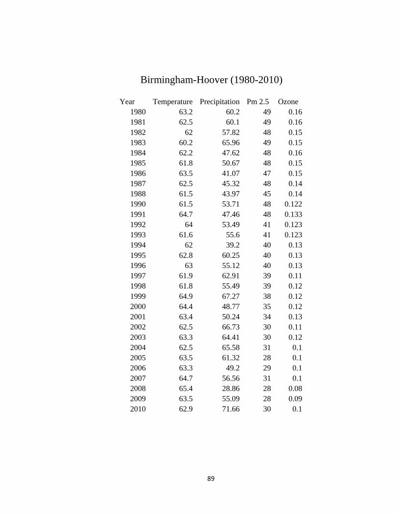
89

Birmingham-Hoover (1980-2010)

Year Temperature Precipitation Pm 2.5 Ozone 1980 63.2 60.2 49 0.16 1981 62.5 60.1 49 0.16 1982 62 57.82 48 0.15 1983 60.2 65.96 49 0.15 1984 62.2 47.62 48 0.16 1985 61.8 50.67 48 0.15 1986 63.5 41.07 47 0.15 1987 62.5 45.32 48 0.14 1988 61.5 43.97 45 0.14 1990 61.5 53.71 48 0.122 1991 64.7 47.46 48 0.133 1992 64 53.49 41 0.123 1993 61.6 55.6 41 0.123 1994 62 39.2 40 0.13 1995 62.8 60.25 40 0.13 1996 63 55.12 40 0.13 1997 61.9 62.91 39 0.11 1998 61.8 55.49 39 0.12 1999 64.9 67.27 38 0.12 2000 64.4 48.77 35 0.12 2001 63.4 50.24 34 0.13 2002 62.5 66.73 30 0.11 2003 63.3 64.41 30 0.12 2004 62.5 65.58 31 0.1 2005 63.5 61.32 28 0.1 2006 63.3 49.2 29 0.1 2007 64.7 56.56 31 0.1 2008 65.4 28.86 28 0.08 2009 63.5 55.09 28 0.09 2010 62.9 71.66 30 0.1

90

Auburn (1980-2010)


1980 62.9 51.62 60 0.15 1981 62 46.62 60 0.15 1982 64 57.8 60 0.15 1983 61.6 62.49 60 0.16 1984 63 43.96 58 0.14 1985 63 45.26 58 0.14 1986 64.8 53.01 59 0.14 1987 63.2 45.43 59 0.14 1988 61.6 53.74 59 0.14 1989 62.3 65.63 59 0.16 1990 65.4 43.43 59 0.15 1991 64.2 54.14 60 0.13 1992 62.6 31.03 60 0.14 1993 64.9 37.43 55 0.13 1994 63.6 57.24 55 0.14 1995 64.6 49.07 53 0.13 1996 63 22.71 53 0.13 1997 62.6 62.92 52 0.13 1998 65.4 49.03 54 0.15 1999 64.6 45.85 54 0.14 2000 63.8 42.4 53 0.16 2001 63.4 50.36 42 0.12 2002 63.9 48 40 0.11 2003 62.8 66.57 34 0.13 2004 63.6 49.06 31 0.13 2005 63 71.32 30 0.13 2006 65 45.67 30 0.1 2007 65.9 28.44 30 0.1 2008 63.2 45.73 28 0.12 2009 62.9 81.58 28 0.11 2010 62.6 45.4 25 0.11

91

Montgomery (1980-2010)


1980 65 75.8 58 0.15 1981 64.8 75.6 58 0.145 1982 64.5 75.46 58 0.142 1983 63.5 75.47 57 0.16 1984 65.3 53.86 57 0.13 1985 65.5 48.34 59 0.13 1986 66.2 52.53 54 0.14 1987 65.1 55.02 54 0.12 1988 64.1 65.43 52 0.11 1990 64.5 75.49 52 0.1 1991 67 53.38 52 0.11 1992 66 67.6 50 0.12 1993 64.1 65.55 50 0.101 1994 64.8 52.94 45 0.12 1995 66.1 59.22 48 0.13 1996 65.6 43.8 47 0.1 1997 63.6 63.09 47 0.1 1998 64.2 47.3 46 0.1 1999 67 44.46 45 0.09 2000 65.7 44.95 42 0.08 2001 64.6 37.95 37 0.101 2002 65.5 47.51 39 0.09 2003 64.6 38.96 40 0.1 2004 66.9 47.86 42 0.1 2005 65.4 49.59 40 0.09 2006 66.1 49.54 42 0.11 2007 66.9 44.71 34 0.09 2008 65.4 36.75 27 0.08 2009 65.2 51.77 21 0.08 2010 64.8 61.41 24 0.09

92

Tuscaloosa (1980-2010)

Year Temperature Precipitation Pm 2.5 Ozone 1980 63.9 66.62 48 0.17 1981 64 41.73 47 0.17 1982 64.7 62.22 47 0.16 1983 62.2 78.35 46 0.1 1984 62.8 46.4 46 6.154 1985 62.8 50.31 47 0.152 1986 64.7 36.04 45 0.122 1987 64 43.29 45 0.12 1988 62.9 51.15 43 0.1 1989 62.8 64.42 45 2.11 1990 65.6 58.31 45 0.11 1991 65.4 55.93 45 0.1 1992 63.2 51.28 41 0.1 1993 63.4 45.93 40 0.1 1994 53 55.3 43 0.12 1995 64.9 58.3 41 0.101 1996 64.3 56.44 41 0.11 1997 64.2 72.17 40 0.12 1998 67.1 60.61 40 0.1 1999 66.3 54.4 40 0.09 2000 66 49.25 38 0.09 2001 65 63.78 36 0.08 2002 65.9 52.62 36 0.08 2003 64.8 62.54 33 0.09 2004 65.2 59.3 35 0.08 2005 66.2 58.43 28 0.08 2006 66.8 55.83 30 0.07 2007 54.9 47.25 27 0.07 2008 64.8 49.66 25 0.06 2009 64.8 75.03 25 0.07 2010 60 48.41 26 0.07

93

Decatur (1980-2010)


1980 66.9 79.7 58 0.16 1981 65.8 72.6 58 0.13 1982 65.5 77.3 57 0.13 1983 66.4 81.5 54 0.14 1984 66.4 73.72 54 0.13 1985 66.9 69.17 57 0.12 1986 67.9 69.34 57 0.101 1987 67.7 67.34 52 0.111 1988 66.3 65.45 56 0.102 1990 65.9 66.25 52 0.1 1991 68.7 55.97 51 0.12 1992 67.8 81.67 51 0.11 1993 66.8 70.46 51 0.1 1994 66.4 62.31 50 0.12 1995 67.5 54.92 45 0.11 1996 66.2 80.49 41 0.1 1997 66.6 66.73 41 0.12 1998 68.6 80.14 41 0.11 1999 68.1 86.52 42 0.12 2000 67.8 61.91 41 0.12 2001 67.4 45.74 40 0.1 2002 67.1 54.65 40 0.11 2003 67.5 72.48 40 0.11 2004 68.1 68.93 38 0.08 2005 67.7 66.16 39 0.09 2006 67.8 63.83 30 0.11 2007 66.8 49.35 30 0.11 2008 66.9 65.25 27 0.1 2009 66.8 69.1 23 0.1 2010 65.3 66.47 21 0.08

94

Dothan (1980-2010)

Year Temperature Precipitation PM2.5 Ozone 1980 63.31 75.91 41 0.16 1981 61.81 51.81 41 0.14 1982 60.51 60.65 40 0.14 1983 61.9 65.39 40 0.12 1984 59.4 77.03 40 0.13 1985 61.4 57.06 38 0.12 1986 60.9 77.57 38 0.11 1987 63.5 57.85 38 0.1 1988 62.4 66.66 37 0.1 1990 61.2 73.58 37 0.1 1991 59.6 72.26 38 0.08 1992 63.2 70.25 38 0.11 1993 62.5 68.6 40 0.11 1994 60.1 68.56 40 0.11 1995 60.4 66.07 37 0.08 1996 61 62.48 37 0.1 1997 60.3 60.18 35 0.1 1998 59.8 57.61 36 0.12 1999 63.7 45.7 30 0.11 2000 62.2 45.69 28 0.11 2001 61.6 42.89 28 0.1 2002 60.5 63.61 28 0.01 2003 62 50.54 27 0.09 2004 60.7 54.87 25 0.09 2005 61.5 59.37 20 0.08 2006 62.8 39.65 20 0.11 2007 60.5 42.59 19 0.11 2008 61.7 28.65 18 0.09 2009 60.5 48.3 18 0.07 2010 59.6 47.7 18 0.07

95

APPENDIX B

Multiple Linear Regression Data

Year Built-up Water other Temperature Precipitation O3(ppm) PM2.5(ug/m3 )1982 28687.35 1422.15 294832 59.9 50.25 0.07 30.21990 28916.4 1367.1 294658 61.2 50.7675 0.106 26.52000 35419.6 1169.91 288352 62.5 54.556 0.13 23.892010 37136.1 1155.42 286650 64.3 56.965 0.1 30.21982 3823.55 833.94 23204 62.3 60.5 0.09 20.51990 3992.92 705.96 23162.62 65.6 60.87714286 0.08 19.12000 5096.34 764.19 22001 66.8 54.229 0.08 18.32010 6073.47 744.97 21043.1 67.8 46.605 0.073 12.41982 5509 4962.6 30096.3 63.2 62.35 0.08 21.41990 5875.07 4793.5 29899.3 66.5 65.70857143 0.087 18.32000 7166.7 4577.67 28823.5 67.5 68.82 0.093 15.52010 12719.3 4445.1 23403.5 68.9 64.396 0.077 9.81982 1501.02 377.46 11034.7 62.3 58.6 0.1 22.31990 2311 163.17 10439.01 63.3 59.4 0.09 21.52000 2531 66.33 10315.9 65.7 59.9 0.07 18.32010 3694.61 58.59 9159.98 67.9 60.2 0.067 11.21982 1729.98 3165.57 13326.2 60.2 50.2 0.064 18.61990 3102.12 2597.83 12521.8 61.5 51.6 0.09 16.22000 3205.66 2305.11 12710.9 66.5 54.2 0.11 15.42010 3519.57 2132.02 12570.2 67.9 56.9 0.07 12.81982 2462.67 489 75124.5 60.2 50.18 0.12 23.201990 7040.79 461 70574.3 61.5 50.37777778 0.09 22.502000 11165 386 66525.2 63.5 54.83 0.11 19.502010 33161.37 267.5 53864.67 64.9 57.71111111 0.08 15.301982 423.18 64.35 7394.31 62.3 49.89 0.12 21.301990 1084.59 35.4 6761.85 63.5 51.737 0.10 20.602000 1288.8 30.6 6562.44 67.4 45.182 0.09 18.502010 1985.31 19.71 5876.82 68.8 53.213 0.08 17.401982 376.85 84.25 9237.12 59.6 64.9 0.12 19.801990 1000.8 65.43 8631.99 60.8 56.95555556 0.09 17.802000 2283.86 32.38 7381.98 62.3 57.74 0.11 16.302010 2928.66 25.32 6744.24 63.2 49.817 0.08 14.601982 3222.36 653.94 17361.9 63.9 66.62 0.075 19.31990 3308.4 617.4 17312.4 64.7 53.222 0.074 15.72000 3712 401 17125.2 65.6 55.961 0.077 13.22010 4210 256.23 16771.97 66.9 57.285 0.06 12.11982 3378.9 650.32 81733.1 61.5 50.4 0.07 30.21990 5868.45 716.04 79177.83 63.3 50.3 0.106 26.52000 6866.91 539.59 78355.8 64.8 54.9 0.13 23.892010 9951.23 422.15 75388.92 68.8 56.2 0.1 30.2

growth of alabama urban areas and its impact on changing

Documents