p sound pressure

N

Fforce

Growth of Loudness for Bone ConductionMaster of Science Thesis in the Master's Programme in Sound and Vibration

MARJA TONTERI TILLGREN

Department of Civil and Enviromental EngineeringDivision of Applied AcousticsVibroacoustics Research GroupCHALMERS UNIVERSITY OF TECHNOLOGYGothenburg, Sweden, 2012Master's Thesis 2012:123

MASTER’S THESIS 2012:123

Growth of Loudness for Bone Conduction

Marja Tonteri TillgrenSupervisors: Alice Hoffmann and Rasmus Elofsson

Department of Civil and Environmental EngineeringDivision of Applied AcousticsVibroacoustics Research Group

CHALMERS UNIVERSITY OF TECHNOLOGYGoteborg, Sweden 2012

Growth of Loudness for Bone Conduction

c� Marja Tonteri Tillgren, 2012

Master’s Thesis 2012:123

Department of Civil and Environmental EngineeringDivision of Applied AcousticsVibroacoustics Research GroupChalmers University of TechnologySE-41296 GoteborgSweden

Tel. +46-(0)31 772 1000

Reproservice / Department of Civil and Environmental EngineeringGoteborg, Sweden 2012

Growth of Loudness for Bone ConductionMaster’s Thesis in the Master’s programme in Sound and VibrationMarja Tonteri TillgrenDepartment of Civil and Environmental EngineeringDivision of Applied AcousticsVibroacoustics Research GroupChalmers University of Technology

Abstract

During the twentieth century the relation between loudness and sound pressure level hasbeen investigated to some extent, but a similar investigation for bone conduction is stillmissing.The aim of this master’s thesis is to investigate the relation between loudness and

excitation level for bone conduction. A listening test has been designed in which themethod of magnitude estimation was used - both with and without an anchor sound. Apure tone at 1 kHz and noise with bandwidth 1 bark band, centered around frequency1 kHz, was used as stimuli. The excitation levels was 20 to 75 dB HL with a step sizeof 5 dB and the number of participants was 34.The listening test resulted in a loudness function that could be approximated to a

power function of intensity with an exponent of 0.2.

CHALMERS, Master’s Thesis 2012

4

Contents

1. Introduction 3

1.1. Background . . . . . . . . . . . . . . . . . . . . . . . . . . . . . . . . . . . 41.2. Scope . . . . . . . . . . . . . . . . . . . . . . . . . . . . . . . . . . . . . . 51.3. Related work . . . . . . . . . . . . . . . . . . . . . . . . . . . . . . . . . . 61.4. What is new? . . . . . . . . . . . . . . . . . . . . . . . . . . . . . . . . . . 9

2. Method 11

2.1. Direct Method versus Indirect Method . . . . . . . . . . . . . . . . . . . . 112.2. Magnitude Estimation versus Magnitude Production . . . . . . . . . . . . 122.3. Absolute versus Relative Method . . . . . . . . . . . . . . . . . . . . . . . 12

3. Listening Test 13

3.1. Participants . . . . . . . . . . . . . . . . . . . . . . . . . . . . . . . . . . . 133.2. Force levels . . . . . . . . . . . . . . . . . . . . . . . . . . . . . . . . . . . 133.3. Signal type and frequency . . . . . . . . . . . . . . . . . . . . . . . . . . . 143.4. Background noise . . . . . . . . . . . . . . . . . . . . . . . . . . . . . . . . 143.5. Test Flow . . . . . . . . . . . . . . . . . . . . . . . . . . . . . . . . . . . . 153.6. Graphical User Interface . . . . . . . . . . . . . . . . . . . . . . . . . . . . 153.7. Test Setup . . . . . . . . . . . . . . . . . . . . . . . . . . . . . . . . . . . . 20

4. Results 21

4.1. Raw Data . . . . . . . . . . . . . . . . . . . . . . . . . . . . . . . . . . . . 214.2. Statistical Analysis . . . . . . . . . . . . . . . . . . . . . . . . . . . . . . . 21

5. Discussion and Conclusion 27

6. Further Work 29

Bibliography 31

A. Calibration of Force Levels 33

A.1. Equipment . . . . . . . . . . . . . . . . . . . . . . . . . . . . . . . . . . . 33A.2. Procedure . . . . . . . . . . . . . . . . . . . . . . . . . . . . . . . . . . . . 34A.3. Results . . . . . . . . . . . . . . . . . . . . . . . . . . . . . . . . . . . . . . 34

B. Derivation of Loudness Function for BC from Equal Loudness Investigation

between AC and BC 37

Acknowledgements

I would like to thank those who supported me in my research process leading to thismaster’s thesis. I would like to express my sincere gratitude to Cochlear BAS for givingme the opportunity to do my master’s thesis at Cochlear BAS. I would like to express myspecial thanks to my supervisors, Rasmus Elofsson and Alice Hoffmann, whose expertiseand support added considerably to the development of my study. Finally I would like tothank all of those who participated in the listening test and made this thesis possible.

2

1. Introduction

In humans sound waves can be transmitted to the cochlea via two different ways: air

conduction (AC) and bone conduction (BC). Sound waves in air are typically trans-mitted via air conduction, while our own voice is transmitted both by air conduction andbone conduction. The transmission path for AC goes through the ear-canal, the tym-panic membrane and the middle ear ossicles into the cochlea[Rei 09]. The transmissionpath for BC goes through the skull bone into the cochlea. Sound waves in air do excitethe skull bone to some extent, but this excitation is very small and for a normal hearingperson it is negligible compared to the AC path. An exception is when we hear our ownspeech. There sound waves are transmitted via AC, but also from the oral cavity to thecochlea directly via the skull bone. In this case what we hear is a combination of bothpaths. This explains why our own voices sound different when heard through recordings.

An important finding in bone conduction physiology research was when von Bekesyin 1932 reported the cancellation of the perception of a bone conduced tone by an airconduced tone[Stn 06]. A conclusion that von Bekesy made was that, although thetransmission to the inner ear is different, the final process for AC and BC stimulationare the same.

For persons with single-sided deafness or certain types of conductive or mixed hearingloss, a bone conduction hearing solutions can be helpful. A BAHA is such a device andit consists of a microphone, a sound processor and an actuator. The microphone picks upsound waves in the air (i.e. pressure fluctuations) and the actuator forwards the soundwith an oscillating force applied to the head. The actuator is usually connected directlyto an osseointegrated1 implant[Car 97] and this type of bone conduction is called direct

bone conduction (DBC). The actuator might also be attached to the head using asoftband and the force is then applied to the head outside the skin. A softband is anelastic band that is attached around the head. The vibrator is then snapped onto anadaptor (a plastic piece) that is a part of the softband. The softband is attached aroundthe head so that the adaptor is positioned on the hard bone just behind the ear - themastoid. Vibration force transferred through the adaptor to the cochlea will - from now- be what is meant when bone conduction (BC) is mentioned in this thesis

1Osseointegration is the formation of a direct interface between an implant and bone, without inter-vening soft tissue.

3

1.1. Background

Force Hearing Level

In hearing by BC the excitation force is usually expressed in terms of force hearing

level (FLHL) and in units decibel hearing level, dB HL. The force hearing level isgiven by the logarithm of the excitation force relative to the hearing threshold for BC:

FLHL = 20 log10

� F

Fth

�dB HL. (1.1)

At 1kH the hearing threshold for BC is 42.5 dB relative to 1 µN[ISO 94]. This gives theforce at the hearing threshold:

Fth = 1µN · 1042.5/20 = 133.35 µN. (1.2)

Loudness

Loudness, N , is the sensation that corresponds most closely to sound intensity[Fas 90].The relation between sensation and physical stimulus can be measured by answering thequestion how much louder (or softer) a sound is heard relative to a standard sound. Theunit is sone; a doubling in sones corresponds to a doubling of loudness. The scale isdefined so that silence approaches 0 sones . And a 1 kHz tone at 40 dB SPL - presentedas a frontal plane wave in a free field - has a loudness of 1 sone.

In psychoacoustics there is another quantity called loudness level and it is importantto distinguish this from loudness. The loudness level, LN , of a sound is defined as thesound pressure level of a 1-kHz tone (in a plane wave and frontal incident) that is asloud as the sound[Fas 90]. Its unit is phon. By comparing sounds of different frequencieswith a standard sound of 1 kHz, equal loudness contours can be measured.

The relation between loudness in sones and loudness level in phons has been deter-mined by a variety of methods in several laboratories[Ste 56]. The median values of theresults obtained can be represented by the equation[Ste 55]:

10 · log10(N) = 0.3 · (LN − 40). (1.3)

This equation was later used in ISO 131-1979 - Expression of Physical and SubjectiveMagnitudes of Sound or Noise in Air [Iso 79]. However, this standard is now withdrawn.

The work in this thesis focuses on loudness.

Steven’s Power Law

In 1955 Stevens publishes a paper[Ste 55] that summarizes data from a number of at-tempts - that were made between 1930 and 1954 - to measure the loudness function forAC. He suggests that for the typical listener the loudness N of a 1 kHz tone can beapproximated by a power function of intensity I, of which the exponent is log10(2). Theequation is: N ∝ I0.30. Sound intensity is proportional to the pressure squared and forAC the law can also be expressed as N ∝ p0.60, where p is sound pressure. The law hold

4

for levels above about 40 dB SPL. Between 30 and 40 dB SPL a vertex can be seen inthe loudness function, and for lower excitation levels the slope of the function is steeper.

The law is later extended (On the Psychophysical Law, 1957) to hold also for otherintensity sensations. The equation is then written as

S = aIk, (1.4)

where S is the magnitude of the sensation, a and k are constants - that are differentfor different type of sensations - and I is the intensity of the stimuli. The equation isdenoted Steven’s power law.

The approach is that Stevens power law can be applied to BC. In this case the factthat intensity is proportional to force squared2 can be used. The listening test that isdescribed in this work measures loudness as a function of excitation force and the resultsgives a number on the constant k for BC .

1.2. Scope

The aim of this work is to investigate loudness sensation as a function of excitation levelfor bone conduction, BC. In hearing by BC the skull bone is excited by a force, F , whileloudness, N , is a subjective quantity. A listening test is designed and implemented tomeasure the relation between the two quantities, i.e. the loudness function for BC.

It is of interest to see if the loudness function can be approximated by a power functionof intensity, as suggested by S.S. Stevens (see Section 1.1):

N = a · Ik, (1.5)

where I is sound intensity and a and k are a constants that are specific for the type ofstimuli. The intensity is proportional to the excitation force squared:

I = b · F 2 (1.6)

Inserting Equation 1.6 in Equation 1.5, and then taking the logarithm, gives the followingrelation between loudness and excitation force:

10 · log(N) = m+ k · 10 · log(F 2), (1.7)

where m is some constant.

The listening test in this study aims to measure k and can not be used to measure m.

2Intensity is work over unit area and work can also be expressed as force times velocity: I = W/A =Fv/A. In terms of impedance this gives I = F 2/ZA. If we assume that the area is constant we getI ∝ F 2.

5

1.3. Related work

The first article by R. P. Hellman, on Growth of Loundess at 1000 and 3000 kHz, de-scribed in this chapter is an investigation of the loudness function for AC. The listeningtest described Section 3 takes a lot of inspiration of one of the methods used in thisarticle, namely the method of magnitude estimation. This method is described furtherin Section 2.2.

The second article, by S. Stenfelt and B. Hakansson, is Air versus Bone Conduction:an Equal Loudness Investigation. If the results from this study are combined withresults from investigations of the loudness function for AC, an estimation of the loudnessfunction for BC can be made.

Growth of Loudness at 1000 and 3000 Hz

Method: Magnitude estimation and magnitude production.Transfer path: AC.Subjects: Students and staff at the university, 9-11 subject in each test design.Test signal: Pure tone.Frequencies: 1000 and 3000 Hz.Amplitudes: 11 different levels between 10 and 100 dB SPL.

Loudness as a function of sound pressure level was measured by magnitude estima-tion and by magnitude production[Hel 76]. In the same study growth of loudness wasalso measured indirectly by loudness matches and by interfrequency matching. No sys-tematic difference in shape of the loudness functions between 1000 and 3000 was found.The results obtained from magnitude estimation and magnitude production can be seenin Figure 1.1. Above about 30 dB SPL the results shows that the loudness functions arepower function of the sound pressure level. This is consistent with Stevens power law,see Section 1.1. The slopes of the curves are slightly different for the two methods. Bycombining the results of the two methods the exponent (previously referred to as k) wasfound to be 0.30 (relative to sound intensity). This holds for levels larger than about 30dB SPL. Below 30 dB SPL the loudness function is steeper.

Air Conduction versus Bone Conduction: an Equal Loudness Investigation

Method: Loudness balanceTransfer path: AC and BC.Subjects: 23 normal hearing and 8 with an hearing impairment.Test signal: Narrow band noise.Center frequencies: 250, 500, 750, 1000, 2000, 4000 Hz.Amplitudes of the AC sound: 30, 40, 50, 60, 70 dB HL.

This artice from 2001, by Stefan Stenfelt and Bo Hakansson, describes a study wereloudness balance testing was conducted between AC and BC. The participants heard

6

674 R.P. Hellman: Growth of loudness at 1000 and 3000 Hz 674

' o z

• •o

_z ol

• orion / / Mogn,tude _Pr_o_duchon • FIE ß 5ooo Hz I / / ß 5ooo Hz

•__j OOl• • 0 I000 Hz ooo SOUND PRESSURE LEVEL IN DECIBELS

FIG. 1. (a) Magnitude estimations of loudness at 3000 and 1000 Hz. Filled and untilled circles indicate group geometric means of loudness estimations at 3000 and 1000 Hz, respec- tively. Vertical bars show the interquartile ranges. (b) Analogous to (a), except that group decibel averages obtained by magnitude production are shown. Interquartile ranges are indicated by the horizontal bars.

SPL produced in the ear canal and in the 6-cc coupler (Shaw, 1966).

Figure l(a) presents loudness estimation data span- ning a stimulus range of nearly 100 dB. Except for their absolute positions, the 1000- and 3000-Hz loudness curves are very nearly the same. Over the mid-to- high intensity range, the data at both frequencies can be approximated by a power function of sound pressure. Above about 30 dB SPL the 3000-Hz data are fitted by a power function with an exponent (slope) of 0.57, and above about 43 dB SPL the 1000-Hz data are fitted by a function with an exponent (slope) of 0.54. Near 40 dB SPL a slight flattening of the loudness function occurs at 1000 Hz but not at 3000 Hz. However, compared to the variability of the loudness estimates, the maxi- mum measured difference of 1.0 dB between the two functions is extremely small and lies within the experi- mental uncertainty. Below 30 dB SPL, as typically found (e.g., Hellman and Zwisocki, 1961), the magni- tude estimation curves at both 3000 and 1000 Hz be- come progressively steeper than a simple power-law prediction.

The relationship of the 3000- and 1000-Hz curves is important for the data points are non-normalized group values obtained on different days. When the stimulus is changed, the listeners are able to adjust their num- ber scale to reflect the observation made by Stevens (1972) that for loudness equality the SPL of a 3000-Hz tone is lower than the SPL of a tone at 1000 Hz.

The 1000-Hz function agrees quite well with respect to slope and position with an earlier binaural curve rePorted by Hellman and Zwislocki (1961). The present curve passes through the point 45 dB SPL and 1.0, whereas the earlier curve passed through the Point 46 dB SPL and 1.0. This small difference in position of i dB further buttresses the point of view that listeners are able to pair loudnesses and numbers on

an absolute basis. Hence it is hardly surprising that in Ward's study (1973), after 1200 trails the standard num- ber 10 assigned to a SPL of 56 dB was eventually ignored and a more appropriate designation of 2.08 was selected by his twelve listeners. What Ward attributed to a time order error can be ascribed to the process of matching numbers with sensation magnitudes described on several occasions by Hellman and Zwislocki (1961, 1963, 1964, 1968) and shown again in Fig. 1.

S.S. Stevens (1975, p. 29) appears to have arrived at a similar conclusion about the method of magnitude estimation. Stevens studied the very first loudness estimates given by a group of 32 listeners in a situa- tion without a standard modulus. He found that the selection of numbers by individual listeners is not a random process; i.e., the number 1 is more apt to be associated with SPL's between 40 and 50 dB than the number 10. Despite the scatter of data, his results show that between 40 and 100 dB SPL the initial esti- mates can be described by a power function of sound pressure with an exponent close to 0.60.

The inverse procedure, magnitude production, also shows that listeners can match loudness to numbers in such a way that the relative loudness of tones at 1000 and 3000 Hz is preserved. Figure l(b) indicates group arithmetic means obtained by magnitude production. Several features of the curves fitted to the points are noted. First, as found using magnitude estimation, the shape of the curves at 1000 and 3000 Hz is similar. Second, over the middle to high intensity range where the curves are linear, magnitude production results in a steeper function than magnitude estimation. This result, ascribed by Stevens and Greenbaum (1966) to a regression effect, has been repeatedly found in mag- nitude scaling experiments. The group means at 3000 Hz obey a power function of sound pressure with an ex- ponent (slope) of 0.66 and the means at 1000 Hz obey a power function with an exponent (slope) of 0.70. Hence, despite the fact that order effects are minimized in the magnitude estimation part of this study, the difference in exponents between the functions generated by mag- nitude estimation and magnitude production is fairly large. Moreover, it is of interest to note that compared to the curves of magnitude estimation, the exponents of the 3000- and 1000-Hz functions obtained by magni- tude production are reversed. This is another ex- ample which illustrates that data obtained using only one procedure rather than a combination of procedures (Stevens, 1969) can be very misleading. Finally, at low SPL's, as noted in the past (Hellman and Zwislocki, 1963), the curve resulting from magnitude estimation is steeper than the one resulting from magnitude produc- tion. Hellman and Zwislocki suggest that the divergence of the two magnitude functions is due to the effect of the threshold boundary. Rowley and Studebaker (1969) also found that the data obtained from magnitude production determine a flatter loudness curve near threshold than do the results of magnitude estimation. They offer another explanation for this effect and attribute it to learning of the magnitude of the smaller numbers used.

To determine whether learning can account for the shape of the magnitude production curve at low SPL's,

J. Acoust. Soc. Am., Vol. 60, No. 3, September 1976

Downloaded 06 Feb 2012 to 129.16.87.99. Redistribution subject to ASA license or copyright; see http://asadl.org/journals/doc/ASALIB-home/info/terms.jsp

Figure 1.1.: The results from magnitude estimation and from magnitude production thatwas performed for AC[Hel 76]. The vertical and the horizontal bars showthe interquartile ranges. The slope of about 0.6 is relative sound pressure.This corresponds to 0.3 relative sound intensity.

one sound through earphones and the task was to adjust another sound, heard througha bone transducer fitted to the subject, for equally loudness by bracketing the standard.The results for the normal hearing group can be seen in Figure 1.2. The levels for the

AC sound is in units dB HL, while the units for the levels of the BC sound is calibratedin such a way that the levels, for AC and for BC, coincide at 30 dB HL. In the article,possible explanations for the difference in growth of loudness between AC and BC arediscussed3. The contraction of the stapedius muscle in the middle ear is mentioned asone part of the explanation. Another part that is mentioned, is distortion from the bonetransducer and tactile stimulations. This especially happens for higher amplitudes atthe lowest frequencies.It seems possible to utilize data presented in the article to calculate a coefficient

for the loudness function for BC. Together with Stevens power law, and the acceptedexponent of 0.30 for AC, such a derivation is made. The result is seen in Figure 1.3 and

3The article does not directly discuss the concept of loudness, but qualitatively this is the discussion.

7

the procedure is explained further in Appendix B. The function in Figure 1.3 is againcalibrated so that the levels coincide at 30 dB HL. The derivation gives the exponent0.33 for the loudness function of BC at 1 kHz.

Fig. 1A presents the results of the loudness balancetest with the narrow-band stimuli centered around 250Hz. The total average increase is 0.80 dB BC /dBAC (S.D.0.11), the lowest value for the normal hearing group inthis investigation. The mean BC increase for every 10dBAC increase is just above 8 dBBC , except at the high-est levels where the increase is only 6.7 dBBC . Fig. 1B,Cshows the results for the stimuli centered around 500Hz and 750 Hz, respectively. The two plots show nearly

the same result : the total average increases are 0.87 and0.88 dB BC /dBAC (S.D. 0.10 and 0.11), the mean BCincreases for every 10 dBAC are around 9 dB BC . Resultswith the stimuli centered around 1, 2, and 4 kHz areplotted in Fig. 1D^F. These three graphs constitutenearly equal results with an overall average increaseof 0.91^0.93 dBBC /dBAC (S.D. 0.07, 0.11, and 0.12).The mean BC increase per 10 dB AC increase is above9 dBBC all over the whole range except at the highest

Fig. 1. The results of the loudness balance test for the normal hearing group. The dots are the individual results (measured at the tens of ACstimuli level) and the crosses spaced along the dotted lines are the BC mean for each level : (A) 250 Hz; (B) 500 Hz; (C) 750 Hz; (D) 1 kHz;(E) 2 kHz; and (F) 4 kHz.

HEARES 3795 5-7-02

S. Stenfelt, B. Ha fikansson / Hearing Research 167 (2002) 1^126

Figure 1.2.: Results that were obtained from the loudness balance test between AC andBC for the normal hearing group[StHa 01]. Individual results are repre-sented by dots. The BC mean for each level is given by the crosses alongthe dotted lines.

8

30 35 40 45 50 55 60 65 70Excitation level, dB HL

10 lo

g 10(N

)

ACBC

Figure 1.3.: The graphs show loudness functions for AC and for BC. The rightmost curveshows how the loudness function for AC, as described by Stevens power lawand the exponent 0.30 (i.e. N ∝ I0.30), looks like. By using the results inFigure 1.2, in combination with this loudness function for AC, the loudnessfunction for BC is derived. The leftmost curve shows this function and itsslope corresponds to an exponent of 0.33.

1.4. What is new?

During the twentieth century the relation between loudness and sound pressure level hasbeen investigated to some extent, but a similar investigation for bone conduction hasnot been made before to that extend. A methodology, that has previously been used tomeasure growth of loudness for AC is here applied to BC. A listening test is designedand implemented for BC. The test is designed in such a way that it could also be usedfor analyzing DBC.

The article Air Conduction versus Bone Conduction: an Equal Loudness Investigationrelates the loudness of a sound heard trough AC with the loudness of a sound heardtrough BC. The outcome of the study suggests that the loudness function might besomewhat steeper for BC than it is for AC. It is of interest to see if an investigation ofthe loudness function, that is performed for BC only, could corroborate this suggestion.

For AC the loudness function on a logarithmic scale, has a slope that can be ap-proximated to a power function of intensity. The power function is often referred to asSteven’s power law. Above about 40 dB SPL the value of the exponent in this power

9

law is accepted as 0.3. Between 30 and 40 dB SPL a vertex can be seen in the loudnessfunction, and for lower excitation levels the slope of the function is steeper. This vertexcoincides with the reference point for the sone scale (1 sone) as suggested by Zwicker &Fastl[Fas 90]. If found in this study, such a vertex point could possibly relate the BCloudness function to the AC loudness funciton.

10

2. Method

In this section some different methods, that can be used to measure growth of loudness,are discussed. The chosen method and the motives behind is presented.

2.1. Direct Method versus Indirect Method

The perception of a psychophysiological stimuli can be measured either directly or in-directly. The method used in this thesis is a direct measurement method. Thatmeans that the ratio of loudness is measured directly by comparing sounds at differentintensity levels. All sounds are heard through BC and the listener is asked to rate theloudness of the sounds.An alternative could be to use an indirect measurement method. Using this

method, the listener would hear sounds both trough AC and trough BC sound. Thelistener is then asked to rate the loudness of the BC sound relative to the AC sound.This method was used in [StHa 01], were the listener was asked to adjust the BC sounduntil it was perceived equally loud as the AC sound.Both methods have their pros and cons. An advantage with the indirect method is

that the results would be calibrated to the sone scale; Let us assume that the listenerhears a tone that has a sound pressure level corresponding to 2 sones. The listeneradjusts a BC sound until it is perceived equally loud as the AC sound. Then it could beassumed that the loudness of the BC sound is 2 sones. However here is a danger. Theresults from measurements of the loudness function for AC differs a lot between differentinvestigations. If this function is just adopted to BC, then the errors will also be adoptedto the loudness function of BC. Furthermore, new errors will be introduce because ofuncertainties in the loudness matching between AC and BC. Let us now assume that asecond listening test is performed in order to relate DBC to BC. Hearing through DBCrequires an implant. A person who has an implant has it because he/she has an hearingimpairment and can either not hear at all through AC, or can only hear poorly throughAC. Therefore DBC can not be compared directly to AC. If the loudness function ismeasured for DBC by using an indirect method, DBC would be compared to BC. Thisextra step would introduce additional errors to the loudness function.An advantage with the direct method is that no errors are adopted from previous

investigation of the loudness function for AC. This method is also easier to implementthan the indirect method, since the setup is more simple and it does not require cali-bration of headphones. Another advantages is that the same method and setup1 can be

1For safety reasons a recommended adjustment of the setup if it should be used for DBC is that agalvanic isolation is used between the power amplifier and the actuator.

11

used for an investigation of the loudness function for DBC.

2.2. Magnitude Estimation versus Magnitude Production

The direct method can basically be divided into two submethods; magnitude estima-

tion and magnitude production. In magnitude estimation the listener hears soundswith different amplitudes and the task is to rate the loudness of the sound. This can forexample be done by asking the subject to assign a number to each sound, correspondingto the loudness of the sound.

In magnitude production the task for the listener is to adjust the stimuli. For examplethe listener is asked to adjust the level of a sound so that it corresponds to a certainnumber. Another approach could be to compare an adjustable sound to a referencesound. The listener could then be asked to adjust the adjustable sound until it isperceived, for example, twice as loud as the reference sound. It has sometimes beennoticed that some intervals are easier to determine than other. For example the intervals’twice as loud’ and ’half as loud’ are known to be easier to determine than other intervals.

In the study described in Section 1.3, both magnitude production and magnitude es-timation was used. Figure 1.1 shows the results of this investigation. The two methodsgave rise to loudness functions with similar shape but with slightly different slopes. Aninterpretation could be that, in magnitude estimation, the subject tends to underes-timate the loudness of the loudest sounds and overestimate the loudness of the softersound.

In the listening test in this work the method of magnitude estimation is used. Themethod is well known and frequently used, which is an advantage. Magnitude estimationis also the fastest method, meaning that many estimates can be made for each force leveland also that more levels can be tested.

2.3. Absolute versus Relative Method

It might be helpful to present a reference sound, a so called anchor sound, to thelistener. The loudness of one variable sound could then be rated relative to the loudnessof the anchor. This is what is meant with a relative method. In the absolute method

no anchor sound is used.Although the listener might experience that the task to rate a sound is easier with an

anchor, it does not necessarily results in better data; the anchor is also a contributingbias. The ear adapts to sounds with different levels, and after hearing a loud sound itis harder to hear a soft sound. This could possible lead to that the loudness of a sound,that is much softer than the anchor, is underestimated. Similarly, the loudness of asound that is much louder than the anchor, might be overestimated.

In the listening test in this work magnitude estimations are made both with andwithout an anchor. To avoid training effects on the loudness estimates, the experimentpart without an anchor was always done first and the anchor sound is first presented inthe last part of the listening test.

12

3. Listening Test

Method: Magnitude estimation - with and without an anchor sound.Transfer path: BC.Subjects: 33 normal hearing.Test signal: Pure tone and noise within one critical band.Frequency/center frequency: 1000 Hz.Amplitudes: 20 to 75 dB HL with a step size of 5 dB.

The listening test is divided into two main parts and a training part in the beginning, seeFigure 3.2. Each part starts with pure tones, Stimulus 1, and ends with noise, Stimulus2. In the beginning is a short trial part where no anchor is used. Part 1 is a repetitionof the trial part but this time more estimates are done and Part 1 also consists of moredifferent amplitudes than the trial part. In the last part, Part 2, an anchor sound is in-troduced. The anchor sound, denoted as Sound 1, has a constant amplitude throughoutthe test and is given the value 100 that represents the loudness of the sound. The othersound, denoted as Sound 2, has a new amplitude for each estimate. The task for thelistener is to estimate the loudness of Sound 2 relative to Sound 1. In Part 1 and Part2 each amplitude and stimulus are repeated twice.

3.1. Participants

Participants were collected through invitations by email to students and staff on Tech-nical Acoustics at Chalmers University, staff at Cochlear BAS and acquaintances in theGothenburg region. Initially 34 people took part of the study. After checking the formthat all participants had to fill in, the data of one participant, who stated him/herselfas sensorineural hearing impaired, was excluded. The remaining test group consists ofparticipants who are between 22 and 46 years old, with a mean of 32 years and a stan-dard deviation of 6 years. All of the participants listed their own hearing as either ’quitegood’, ’good’, or ’very good’.

3.2. Force levels

It is desirable that the range of amplitudes is as big as possible, but there are somelimitations. The lowest possible amplitude that might be of interest to test is the hearingthreshold and the highest amplitude to be tested must be lower than any amplitude thatmight cause damage to the test persons hearing. Further limitations are given by thecharacteristics of the actuator and of the electrical components in the setup. For high

13

amplitudes distortion occurs due to nonlinearities in the apparatus and for very lowamplitudes the signal to noise ratio is low, since the signal is then closer to the noisefloor. Figure 3.1 shows total harmonic distortion, THD, of the actuator as the functionof the voltage in to the actuator, Uact. The lowest level in the listening test (20 dBHL) is achieved for Uact ≈ −40 dB rel. 1 V. The THD is then about 2%. The highestamplitude (75 dB HL) is achieved for Uact ≈ 15 dB rel. 1 V, corresponding to a THD ofabout 11%. For details about the calibration of the force levels, see Appendix A.

3.3. Signal type and frequency

Two different types of signals are used in the listening test; a pure tone at 1 kHz and noisewith a bandwidth of one bark band centered around frequency 1 kHz. The frequency of1 kHz is chosen since it is a commonly used test frequency. It is also unusual to have ahearing loss around this frequency. A pure tone might however result in modal shapesinto the human head. The vibration amplitude of a pure tone may for some subjects begreatly affected by a resonance or mode, whilst for others not. To mitigate undesiredeffects from resonances, noise - which is less prone to cause inter-subject differences - isutilized. Noise consisting of frequencies within one bark band mainly excites hair cells,in the cochlear, within one critical band. Theoretically the noise signal and the puretone should give rise to similar loudness functions if the energy in both signals is thesame.

A butterworth digital filter, with a lower frequency of 920 Hz and an upper frequencyof 1080 Hz, is used in Matlab to create the noise. A vector with uniformly distributedpseudorandom numbers1 was filtered through this filter. To avoid clipping the signal isramped up, respectively ramped down, during 125 ms. A hanning window split into twopieces was used for this purpose. The total length of the signal was 1 second.

3.4. Background noise

Part of the listening test was performed at at Applied Acoustics, Chalmers University,and part of it was performed at Cochlear BAS. In both cases the test was performed ina room with good sound isolation and with short reverberation time. The backgroundnoise was roughly the same in both rooms. In one of the rooms it was measured asLAeq = 24 dB SPL at listeners position by using a sound level meter2. The actuator wasenveloped by a plastic housing to avoid sound radiation, but at high force levels it wasstill possible to hear sound radiation from the actuator. At the lower amplitudes thestrongest noise source was the sound of the clicking of the computer mouse. The SPLfrom this click, inside the test room, was measured as LApeak = 68 dB SPL at listenersposition.

1The command rand was used in Matlab.2Hand-held Analyzer 2250 Light from Bruel & Kjær.

14

Figure 3.1.: Total harmonic distortion of the actuator as a function of the voltage to theactuator, Uact.

3.5. Test Flow

Figure 3.2 shows the overall algorithm of the listening test. Each part (Part 1 and Part2) consists of 12 different levels that are repeated 4 times. In the two first repetitionsa pure tone is heard and in the two latter repetitions narrow band noise is heard. Theorder of the twelve levels are random for each repetition. The only limitation of therandomization is that the first stimuli in the first repetition is not allowed to have themaximum level of 75 dB HL. The training session in the beginning consists of five levelsand two repetitions. In the first repetition the stimulus is a tone and in the secondrepetition it is narrow band noise. Figure 3.3 shows the algorithm that is repeated foreach new stimuli, i.e. for each new level of the sound.

3.6. Graphical User Interface

The GUI for Part 1 of the listening test is seen in Figure 3.4 and 3.5. When the button’Listen’ is pressed the stimulus is heard during one second. A number that representsthe loudness of the stimulus is filled into the grey box. When ’Enter’ is pressed, on thekeyboard of the computer, the button ’Next’ appears. For each new level the listenercan press ’Listen’ as many times as desirable but as soon as the button ’Next’ is pressed

15

Stimulusi

presented

Subject inputs estimate

of N

Subject confirms estimate

Trainingsession

Part 1:absolute

Part 2:relative

12!4

12!4

5!2

Figure 3.2.: The overall algo-rithm for the lis-tening test.

Stimulusi

presented

Subject inputs estimate

of N

Subject confirms estimate

Trainingsession

Part 1:absolute

Part 2:relative

12!4

12!4

5!2

Figure 3.3.: Algorithm thatis repeatedfor each newstimulus.

it is not possible to go back to the previous estimate.In Part 2 the design is slightly different, see Figure 3.6 and 3.7. This time an anchor

sound, that has constant amplitude throughout the whole listening test, is presented.The anchor sound is called ’Sound 1’ and the variable sound is called ’Sound 2’. Theanchor sound is assigned the value 100 that represents its loudness. The listener is askedto rate the loudness of Sound 2 relative to Sound 1.

Two versions of the GUI exist; one Swedish version and one English version. Theenglish version is shown in Figure 3.4 - 3.7. The visual design of the Swedish version isthe same as for the English version, but the text is replaced with text in Swedish, seeTable 3.1. Three participants used the English version of the listening test and all otherparticipants used the Swedish version.

16

Table 3.1.: The written text in the English and the Swedish version of the listening test.Figure 3.4 - 3.7 show the text in its context.

English version Swedish version

Listen LyssnaNext NastaSound 1 Ljud 1Sound 2 Ljud 2Assume that Sound 1 has a loudness Anta att ljudvolymen for Ljud 1 arof 100 . What loudness does Sound 2 100. Mata in den ljudvolym som duhave? Type in the fitting number, anser galler for Ljud 2 i rutan nedan.then press Enter. Tryck sedan pa Enter pa tangent-

bordet for att uppdatera vardet.You perceived the loudness of Du anser att ljudvolymen for Ljud 2 arSound 2 as xxx . If this number fits xxx . Stammer det? Tryck i sa fall payour perception press Next. If it does Nasta. Om det inte stammer, vanligennot fit, please change the number mata ni ett nytt varde och tryck sedanand press Enter. pa Enter.Type in a number that represents the Mata in en siffra som du anserloudness of the sound you heard. motsvarar ljudvolymen pa det ljud duPress Enter on the keyboard to horde. Tryck sedan pa Enter pa tan-proceed. gentbordet for att uppdatera vardet.You perceived the loudness of the Du anser att ljudvolymen pa det ljudsound as xxx. If this number fits your du horde motsvaras av siffran xxx.perception press Next. If it does not Stammer det? Tryck i sa fall pafit, please change the number and Nasta. Om det inte stammer, vanligenpress Enter. mata ni ett nytt varde och tryck sedan

pa Enter.

17

Figure 3.4.: This is how the GUI looks like in Part 1 - and also during the training part- each time a new stimulus is presented to the listener.

Figure 3.5.: When a number is filled into the grey box, and ’Enter’ is pressed on thekeyboard on the computer, the GUI is updated. Note that the number ’120’is just an example of a number that the listener might fill into the box.

18

Figure 3.6.: This is how the GUI looks like in Part 2 each time a new stimulus is presentedto the listener.

Figure 3.7.: When a number is filled into the grey box, and ’Enter’ is pressed on thekeyboard on the computer, the GUI is updated. Note that the number ’30’is just an example of a number that the listener might fill into the box.

19

3.7. Test Setup

The subjects sit on a chair, in front of a computer on a table, in a quiet room. Theactuator is attached to the mastoid (hard bone) behind one of the subjects ear, using asoftband. The softband is tightened so that it is not too loose but not so tight that itis uncomfortable for the listener. The static force of the plastic piece (on the softband)on the mastoid was about 2 - 3 N. The subject hears all sounds through the actuatorand uses mouse and keyboard to navigate through the test on the computer. Figure 3.8shows the setup. The following equipment was used:

• Computer, mac book pro with Matlab

• Sound card, Edirol FA-66

• N4L Laboratory power amplifier LPA01

• Actuator, Baha Cordelle II Headworn, serial no: 0801597

• Softband

• Cables

Computer

FA-66 LPA01

firewire

Cordelle II

Subjectinput on keyboard / mouse clicks

Softband

Figure 3.8.: Setup during the listening test.

20

4. Results

4.1. Raw Data

The raw data of the listening test is shown in Figure 4.1. The data consists of thenumbers that were assigned to the stimuli by the listeners.

10 20 30 40 50 60 70 8010−1

100

101

102

103

104

Force Hearing Level, dBHL

Subj

ect L

oudn

ess

Estim

ate

Listening Test Data

Relative (with anchor), stimulus 1 (tone)Relative (with anchor), stimulus 2 (noise)Absolute (no anchor), stimulus 1 (tone)Absolute (no anchor), stimulus 2 (noise)

Figure 4.1.: Raw data of the listening test. Each mark (dot or cross) represents onesingle estimate.

4.2. Statistical Analysis

Data from 33 participants is analyzed. For a few estimates the listener has answeredwith the number zero, meaning that the listener could not hear the sound. If the soundcan not be heard, its loudness can not be rated and these estimates have therefore beenexcluded from the analysis.

21

Figure 4.2 shows the geometric means of the data from the listening test. Thegeometric mean of a vector with n elements is given by the n-th root of the productof all elements in the vector. In the same figure vertical bars indicates inter quartile

ranges, that is the difference between the upper and the lower quartiles.Regression analysis is used to fit straight lines to the geometric means of the data, see

Figure 4.3. Logarithmic scales were used, so that the x-axis represents 10 · log10(F 2/F 2th)

and the y-axis represents 10 · log10(N). In this plot the slope of the lines correspondsto the exponent in Stevens power law. The data was also analyzed using the statisticalsoftware Minitab. Values obtained for the exponent k are seen in Table 4.1.

To calculate the confidence intervals t-distribution was assumed. The degree offreedom, df , i.e. the number of estimates per signal type and test design, is df � 120which gives kα = 1.96. The analysis in Minitab gives values on the standard error, SE.The confidence interval is then given by the formula

CI = ±kα · SE, (4.1)

where SE is specific for the degree of uncertainty that is required. The values of CI fora 95% confidence interval can be seen in Table 4.1.

The same procedure is repeated, but this time straight lines are fitted to smallerintervals of the data; one line is fitted for the data between 20 - 35 dB HL, anotherbetween 40 - 55 dB HL and a third between 60 - 75 dB HL. The exponent of theloudness function is derived for each of these intervals and can be seen in Table 4.2.

The exponent obtained from the analysis over the total range (20-75 dB HL) is closeto 0.2 for both stimuli and for both test designs. But when the data is analyzed inintervals different exponents are obtained for different intervals. This is especially clearfor the relative test design, where an anchor at 47.5 dB HL was used; in this case theloudness function is much more flat around the anchor point and steeper far away fromthe anchor.

The squared correlation coefficient, R2, answers, in short, the question ’how goodis the line in fitting the data point?’. It measures the variation in the samples relativeto the total spread. The squared correlation coefficient is defined as[Arv]

R2 = 1− SSE

SSyy

=

�n

i=1(yi − yi)2�n

i=1(yi − yi)2. (4.2)

In this equation SSE is the sum of the squared differencees of the actual value, y, andthe value predicted by the regression line, y. SSyy is the sum of the squared differencesof the actual value, y, and the average value y.

Analysis of variance (ANOVA) was used on the the absolute estimation test data,including both force level and subject in the model, which resulted in values of R2 =91.21% for Stimulus 1 and R2 = 92.31% for Stimulus 2. This implies that the seeminglylow R2 values in Table 2 for the absolute estimation data is due to individual offset inloudness scale, not a poor linear fit with respect to slope of the loudness function.

All analyzes, and both test designs, gives a somewhat higher value on the coefficientk for the stimuli 2 (noise) than for stimuli 1 (tone). The difference is especially clear

22

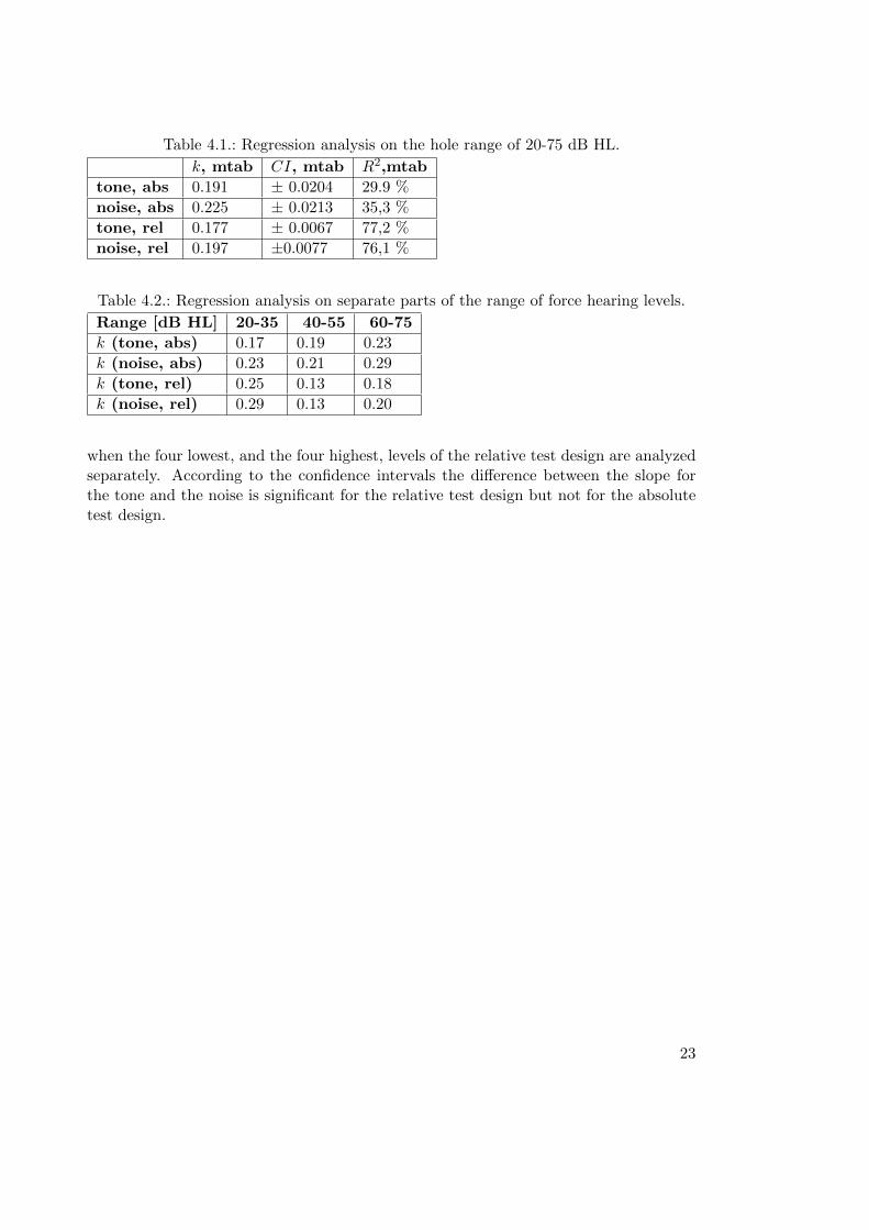
Table 4.1.: Regression analysis on the hole range of 20-75 dB HL.

k, mtab CI, mtab R2,mtab

tone, abs 0.191 ± 0.0204 29.9 %noise, abs 0.225 ± 0.0213 35,3 %tone, rel 0.177 ± 0.0067 77,2 %noise, rel 0.197 ±0.0077 76,1 %

Table 4.2.: Regression analysis on separate parts of the range of force hearing levels.

Range [dB HL] 20-35 40-55 60-75

k (tone, abs) 0.17 0.19 0.23k (noise, abs) 0.23 0.21 0.29k (tone, rel) 0.25 0.13 0.18k (noise, rel) 0.29 0.13 0.20

when the four lowest, and the four highest, levels of the relative test design are analyzedseparately. According to the confidence intervals the difference between the slope forthe tone and the noise is significant for the relative test design but not for the absolutetest design.

23

10 20 30 40 50 60 70 80100

101

102

103

Force Hearing Level, dBHL

Subj

ect L

oudn

ess

Estim

ate

Listening Test Data

Geometric mean, relative (with anchor), stimulus 1 (tone)Geometric mean, relative (with anchor), stimulus 2 (noise)Geometric mean, absolute (no anchor), stimulus 1 (tone)Geometric mean, absolute (no anchor), stimulus 2 (noise)

Figure 4.2.: Data from the listening test. The bold symbols (square, circle, diamond andcross) shows the geometric mean of the data. The vertical bars indicatesinter quartile ranges. Stimulus 1 is a pure tone at 1 kHz and Stimulus 2 isnoise with bandwidth 1 bark band around center frequency 1 kHz.

24

20 30 40 50 60 70 800

5

10

15

20

25

30

Force Hearing Level, db HL

10 lo

g 10(N

)

Absolute (no anchor), toneAbsolute (no anchor) noiseRelative (with anchor), toneRelative (with anchor), noise

Figure 4.3.: Data from the listening test. The data point shows the geometric mean ofthe data and the dotted lines are curves fitted to these geometric means. Theslope of the curves are: k = 0.19 for Stimulus 1 without anchor, k = 0.23for Stimulus 2 without anchor, k = 0.18 for Stimulus 1 with anchor andk = 0.20 for Stimulus 2 with anchor.

25

26

5. Discussion and Conclusion

The exponent obtained from the regression analysis over the total range (20-75 dB HL)is close to 0.2 for both stimuli and for both test designs. Since both stimuli is within thesame critical band it is expected that they should give rise to similar loudness functions,which is consistent with these results.When the data is analyzed in intervals different exponents are obtained for different

intervals. This is especially clear for the relative test design, where an anchor is used;in this case the loudness function is clearly more flat around the anchor point (47.5 dBHL) and steeper on the sides. The loudness function for AC shows a vertex so that thefunction is steeper below about 30 dB SPL. For the relative test design in this work thedifferences in slope between the different intervals show a similar behavior. However,this vertex is not seen in the absolute test design, indicating that the vertex occurs asan effect ofbias. The most obvious bias in this case is the anchor sound.In the relative test design the squared correlation coefficients indicates that 77 %

respectively 76 % of the data, for the tone respectively for the noise, can be explainedby a linear relation between 10 · log10(N) and force hearing level. For the absolute testdesign the corresponding portion is much lower. This is due to the fact that differentlisteners used different scales, resulting in a much bigger range of answers. If this fact istaken into account, which is made when the ANOVA is made, the squared correlationcoefficients are instead much higher for the relative test design than they are for theabsolute test design. In this case they indicates that 91 % respectively 92 % of the data,for the tone respectively for the noise, can be explained by a linear relation.The accepted exponent of the loudness function for AC is 0.30. The results from the

equal loudness investigation between AC and BC, that was made by B. Hakansson andS. Stenfeldt (see Section 1.3), indicates that the loudness function is steeper for BC thanit is for AC. The calculations made in Appendix B estimates the exponent for BC as0.33 while the results from the listening test implies that the exponent is about 0.2 forBC. How can this apparent contradiction be explained?There tend to be a difference between the loudness functions that are measured with

magnitude estimation and magnitude production respectively. In the measurement ofthe loudness function for AC at 1000 Hz and at 3000 Hz, see Section 1.3, the exponentobtained for 1 kHz by magnitude production was 0.35, while it was 0.27 when it wasobtained by magnitude estimation. This could explain part of the discordant results,but is not enough as a single explanation.If an essential difference could be found, between the method used in this investigation

and the method that was used to measure the loudness function for AC, this could bea possible explanation of the discordant. The method, that is used in the listeningtest in the present study, appears to be very close to the method that is used in the

27

measurement of the loudness function for AC at 1000 Hz and at 3000 Hz. In bothmeasurements magnitude estimation is used, both measurements uses a relative methodand in both cases the data from the first set of estimates is thrown away. A differenceis however that in the present investigation the listener was clearly informed about thatthe first set of estimates is seen as a trial part, which does not seem to be the case in theprevious investigation. Another difference is that in the AC measurement a bigger rangeof amplitudes is used than in the BC measurement. The range of amplitudes used in theAC measurement was 10 - 110 dB SPL with a step size of 10 dB, while the levels used inthe present investigation is 20 dB HL - 75 dB HL with a step size of 5 dB. None of thesedifferences in test design seem to give an evident explanation of why a steeper loudnessfunction is obtained in the previous investigation than in the present investigation.

The next question is then if a meaningful disparity, between the listening test in thiswork and the listening test by Hakansson and Stenfeld, can be found? One thing tonotice is that, in the equal loudness investigation between AC and BC, the signal wasalternated so that the listener constantly heard a sound - either through AC or throughBC. In the present investigation only sound heard through BC is used. If and how thiscould possible affect any results is left to the reader as a little exercise.

28

6. Further Work

To reproduce the listening test that is described in this work, but to do it for AC, wouldgive important information. If it is found that the results give rise to an exponent kthat is lower for AC than for BC - which would be consistent with the equal loudnessinvestigation described in section 1.3 - it indicates that the methodology is the crucialpoint. If the results, on the other hand, shows that the loudness function is steeper forAC than for BC it gives a reason for further investigations.

29

30

Bibliography

[Ste 55] The Measurement of Loudness, S. S. Stevens (Psycho-Acoustic Labora-tory, Harvard Univesity), The Journal of the Acoustical Society of Amer-ica, Vol 27 Issue: 5 , pp 815-829, 1955.

[Ste 56] Calculation of the Loudness of Complex Noise, S. S. Stevens (Psycho-Acoustic Laboratory, Harvard Univesity), The Journal of the AcousticalSociety of America, Vol 28 Issue: 5 , pp 807-832, 1956.

[Hel 76] Growth of Loudness at 1000 and 3000 Hz, Rhonoa P. Hellman, Laboratoryof Psychophysics, Harvard University, Massachusetts 02138, 1976.

[Iso 79] ISO 131-1979, Physical and Subjective Magnitudes of Sound or Noise inAir, 1979. Note: withdrawn.

[Hak 89] Skull Simulator for Direct Bone Conduction Hearing Devices. Hakansson,B. and Carlsson P (Department of Applied Electronics, Chalmers Unev-ersity of Technology, Goteborg, Sweeden). Scand Audiol 1989, 18 (91-98)

[Fas 90] Psychoacoustics - Facts and Models, 3rd Ed., Springer Verlag, H. Fastland E. Zwicker,1990.

[ISO 94] ISO 389-3 Acoustics - Reference zero for the calibration of audiometricequipment - Part 3: Reference equivalent threshold force levels for puretones and bone vibratiors, 1st ed., 1994.

[Car 97] The Bone-Anchored Hearing Aid: Reference Quantities and FunctionalGain, Peder U. Carlsson and Bo Hakansson, Ear & Hearing, 1997;18;34-41.

[StHa 01] Air versus Bone Conduction: an Equal Loudness Investigation, StefanStenfelt ∗, Bo Hakansson (Department of Signals and Systems, ChalmersUniversity of Technology), Hearing Research Volume: 167 Issue: 1-2Pages: 1-12, 2001

[AFS 05] Arbetsmiljoverkets Forfattningssamling - Buller (AFS 2005:16), Ar-betsmiljoverket, Sweden, 2005.

[Stn 06] Simultaneous cancellation of air and bone conduction tones at two frequen-cies: Extension of the famous experiment by von Bekesy, Stefan Stefelt,Department of Neuroscience and Locomotion, Division of Technical Au-diology, Lindkoping University, Sweden, 2006.

31

[Rei 09] Bone Conduction Hearing in Human Communication - Sensitivity, Trans-mission, and Applications, Sabine Reinfeldt, Division of Biomedical Engi-neering Department of Signals and Systems, Chalmers University of Tech-nology, Gothenburg, Sweden, 2009.

[Arv] Regression Analysis, lecture slides by Martin Arvidsson, Division of Qual-ity Sciences, Department of Technology Management and Economics,Chalmers University of Technology.

32

A. Calibration of Force Levels

The force hearing level of the actuator on an artificial mastoid, Fact, as a function ofnumerical unit in Maltab, NU , is measured. An artificial mastoid is a mechanical system,with a built-in force transducer, that designed for measurements of the of the force of anactuator. The system is designed to simulate a situation where the actuator is attachedoutside the skin on the hard bone just behind the ear, i.e. the mastoid.

A.1. Equipment

The following equipment is used.

• Computer, Mac book pro

• Sound card, Edirol FA-66

• N4L laboratory power amplifier LPA01

• Baha Cordelle II Headworn, serial no: 0801597

• Softband

• Cable ties

• Artificial mastoid Type 4930, Bruel & Kjaer, serial no: 2733777, calibration dueOct. 2011

• Newton meter

• PC with Matlab

• Sound card DT9837A

• FLUKE 112 True RMS Multimeter

The artificial mastoid meets the requirements specified in IECR373, BS 4009 (1975),and ANSI S3.26-1981.

33

A.2. Procedure

The measurement setup can be seen in Figure A.1 . A pure tone at 1 kHz, and withnumerical amplitude NU , is crated in Matlab on the mac. The spectrum of the electricalsignal from the artificial mastoid, and also the electrical signal into the actuator, ismeasured using the sound card DT9837A and a Matlab program on the PC, writtenby Rasmus Elofsson (2012). A calibration of the artificial mastoid is imported intothe program so that the signal to CH1 is monitored as force, Fact. The signal intoCH2 is monitored as voltage, Uact. The spectrum of the signals are analyzed in narrowbands and by using a steady-state, linear spectrum with a frequency resolution of 10Hz, Flattop window. To validate the measurement the signal into the actuator, Uact wasalso measured using a voltage meter.

The data from the measurement is then used to calculate a calibration factor corre-sponding to the relation between numerical unit and force hearing level. The calibrationfactor is implemented in the listening test (Matlab program). The force of the actuatoris then measured in a second measurement, using the numerical amplitudes in the lis-tening test program that is expected to correspond to the hearing levels 20, 30, 40, 50,60, 70, ( 75) dB HL. The same measurement is done both for a pure tone at 1 kHz andfor noise within one bark band with center frequency 1 kHz. In the measurement of thenoise signal the data is analyzed in 3rd octave bands.

A.3. Results

The results from the first measurement of Fact and Uact is seen in Table A.1. The resultsshow a linear dependency over the hole range of amplitudes. The ratio between the rmsvalue of the force, Fact, and numerical unit, NU , (top value) is calculated as

Fact

NU= 2.7558. (A.1)

The voltages that are measured with the voltage meter agree with the voltage that ismeasured using the Matlab program. The deviation between the two measurement is ≤3% and can be explained by the limitations in digits of the voltage meter. For higherlevels, where more digits were displayed, the accuracy is better.

The results of the measurement that is made to confirm that the calibration factoris implemented correctly in the listening test program are seen in Table A.2. The mea-surement show that for both tone and noise signal the error is ≤ 0.3 dB.

34

Table A.1.: Measured force and voltage for a pure tone at 1 kHz with numerical ampli-tude NU in the Matlab program.

NU 0.0005 0.001 0.01 0.02 0.05 0.1 0.2 0.3 [-]

Uact 10.30 20.6 206.1 412.2 1030 2061 4121 6180 [mV]

Fact 1.245 2.506 25.8 51.88 127.8 257.0 516.9 763.4 [mN]

FLHL 19.40 25.48 45.72 51.80 59.63 65.7 71.77 75.16 [dB HL]

Table A.2.: Force hearing level measured for verification. In this table the force hearinglevels are measured directly from the signal that is given by the listeningtest program and setup.

FLHL(expected) 20.00 30.00 40.00 50.00 60.00 70.00 75.00 [dB HL]

FLHL (tone, measured) 20.00 30.08 40.20 50.30 60.29 70.18 — [dB HL]

FLHL (noise, measured) 19.7 29.8 39.9 50.1 60.2 70.3 75.0 [dB HL]

Figure A.1.: Setup during the measurement of Fact and Uact.

35

36

B. Derivation of Loudness Function for BC

from Equal Loudness Investigation

between AC and BC

The graph in figure 1.2 gives the following relation:

10 · log�F 2

F 20

�= 0.92 · 10 · log

�p2

p20

�, (B.1)

where F is the excitation force, p is sound pressure, p0 is the sound pressure correspond-ing the the hearing threshold for a 1 kHz AC tone and F0 is define in such a way thatthe two graphs coincide at SPL 30 dB HL.Put now F/F0 = Ftemp and p/p0 = ptemp. This gives

1

0.92· log(F 2

temp) = log(p2temp) (B.2)

⇒ F 2/0.92temp

= p2temp. (B.3)

Stevens power law states that:

N = a · (p2)0.3 ⇒ N = b · (p2temp)0.3, (B.4)

where a and b are constants. Inserting Equation B.3 in Equation B.4 gives

N = b · (F 2temp)

0.3/0.92 = c · (F 2)0.33, (B.5)

where c is a constant.∴ N ∝ (F 2)0.33. (B.6)

37